3.1.1. Three-Dimensional Feature Parameter Calculation
The core elements of ARCG are seed point selection and growth criteria determination. These steps must be quantified using 3D spatial features. Therefore, this study employs normal vectors and curvature as the key characterization parameters.
- (1)
Normal Vector Calculation
While PCA (Principal Component Analysis) efficiently computes normal vectors for large-scale point clouds by evaluating data trends through eigenvalues, its neighborhood matrix construction tends to smooth normal vectors at sharp rock discontinuities, causing distortion. To address this, we implement Robust Randomized Hough Transform [
43], which significantly improves normal estimation robustness at discontinuities.
As depicted in
Figure 4, Robust Randomized Hough Transform also initiates computation from neighborhood points (the arrows in the figure indicate the normal vectors of the corresponding planes). As illustrated, its distinctive feature involves the following: within a given central point’s neighborhood, randomly selecting two non-collinear points (
,
) to form a triplet with the center point. This triplet constitutes a computational unit, where the cross product of internal edge vectors
and
yields the unit’s normal vector
(where
,
). To record the distribution of normal vectors, we adopt a spherical accumulator for statistical convenience, following the comparative analysis of different accumulators [
44]. As more triplets are constructed, the resulting normal vectors increasingly approximate a normal distribution. However, the number of possible triplets in a point set scales cubically with the number of points (≈n
3). Thus, when the normal vector distribution stabilizes within a specific range, we terminate triplet generation and proceed to the next target point, assuming convergence to the correct normal vector. Here are some important definitions: Let
be the number of accumulator grid cells,
be the number of triplets. For the current grid cell
and triplet
, they satisfy an independent statistical distribution
, where
= 1 when vote is assigned to triplet
, and
= 0 otherwise. Furthermore, Let
be the empirical mean value of votes for grid,
be the true value,
be the distance between two,
be the confidence score,
be the minimum triplet threshold (stopping criterion). The relationship between
and
is given by the following empirical formula:
By applying Hoeffding’s inequality to Equation (1), we derive the probabilistic relationship between the
and the aforementioned parameters as follows:
The construction process terminates when the triplet count satisfies , whereupon the grid cell with the highest accumulator votes is selected, and its mean value is adopted as the target point’s final normal vector. To mitigate grid discretization effects during voting—where the distribution peak may coincide with grid boundaries—we implement an accumulator rotation strategy. Experimental results demonstrate that five rotations with 5° increments effectively neutralize this artifact.
- (2)
Curvature Calculation
While conventional curvature computation relies on surface polynomial fitting, this study adopts normal vector variation within local neighborhoods to quantify curvature—achieving more precise 3D curvature characterization while maintaining explicit relationships with normal vectors. As formalized in Equations (3) and (4) as follows:
where
denotes the normal vector of the target point,
represents the normal vector of any neighboring point,
indicates their included angle, and
specifies the neighborhood point count.
3.1.2. Adaptive Region Contour Growing
Region growing and plane fitting methods are widely used for individual discontinuity segmentation. Originally developed for image segmentation, region growing algorithms identify areas of interest based on user-defined criteria. This approach proves particularly suitable for rock mass discontinuities due to their distinct planar characteristics. Compared to static iterative formulas in surface fitting, user-defined growth criteria better preserve geometric details of discontinuities. However, traditional region growing requires manual selection of multiple thresholds. This often leads to discontinuities being prone to over-segmentation or under-segmentation, and requires continuous parameter tuning through trial and error to achieve satisfactory results. Furthermore, after completing the segmentation of a single plane, the extraction of the discontinuities contour—also a crucial step for characterizing its 3D morphology—increases the time cost when these steps are executed sequentially. To address this limitation, we propose an adaptive thresholding method, Adaptive Region Contour Growing, that automatically identifies discontinuity by specifying only the value ranges for normal vectors and curvature thresholds. This study introduces another key enhancement: conventional point-cloud contour extraction methods exhibit significant limitations when handling concave discontinuities with complex geometries. Current approaches (e.g., alpha shape, convex hull, Delaunay triangulation, and meridian-parallel scanning) fail to simultaneously address manual parameter tuning requirements, and mixed convex-concave boundary preservation. Moreover, these methods typically require complete discontinuity segmentation before contour extraction. To overcome the rigidity of fixed thresholds and cumbersome post-processing, we propose a mobile spatial contour scanning method integrated with adaptive region growing. This simultaneously performs complex discontinuity identification, and contour point cloud extraction. By eliminating the need for full-discontinuity participation in intersection calculations, computational efficiency is significantly improved. The methodology ARCG comprises the following:
Step 1: The algorithm initiates by sorting all computed curvature values in ascending order and selecting the point with minimum curvature as the initial seed point
Step 2: For each neighboring point , two growth criteria are sequentially evaluated: the angle between ’s normal vector and ’s normal vector—if exceeds a predefined threshold , is classified as a pending point , otherwise it is added to the seed queue;
Step 3: Evaluate the other growth criteria: curvature difference , if it is below threshold , becomes an accessory seed point , otherwise it is marked as a boundary point .
Step 4: Upon encountering , the algorithm records it as the current contour point and calculates its projection vector with the initial seed point onto the plane defined by ’s normal.
Step 5: Subsequent boundary point undergo vector comparison: if and the inter-vector angle is below threshold, replaces ; otherwise, it is appended as a new contour point.
Figure 5 illustrates the parallel processing pipeline for region growing and boundary point extraction.
To handle complex concave polygons, after completing boundary point scanning, we project the regional points onto a 2D plane centered on the initial seed point and randomly partition subspaces. When encountering discontinuous boundary points within a subspace characterized by small-angle projection vectors with significant modulus differences, the system identifies boundary point defects. Since the discontinuity has already undergone preliminary segmentation, we then apply K-means++ clustering to divide the point cloud into two clusters. The cluster centroid farther from the initial seed point becomes the new scanning location. The newly acquired boundary points merge with original points after deduplication to form the final boundary point set.
Notably, to enable dynamic adjustment of the normal vector threshold, we define an adaptive threshold
(Equation (5)):
where
and
denotes the prescribed maximum and minimum threshold bounds,
represents the current regional point count, and
is a scaling factor controlling the growth rate, its value is related to the point cloud density and the size of the currently grown region. Here, the
is defined as the square of the ratio between the maximum distance between any two points in the current region and the average point spacing. When the region begins to grow, a strict angular tolerance (
) is maintained, close to
. When the region becomes sufficiently large, the tolerance
is appropriately relaxed according to Equation (5).
The adaptive curvature threshold
follows Equations (6)–(10):
where
is the curvature value set
within the current region,
represents the prescribed lower curvature threshold bound;
represents the regional consistency factor, where
represents the standard deviation of curvature within the current region and
represents the global standard deviation of curvature;
represents the neighborhood connectivity factor, where
represents the average neighborhood connectivity count;
represents the curvature distribution skewness factor, where
is the mean curvature within the current region and
is the median curvature within the region.
A critical observation is that during region growing, normal vectors determine point inclusion while curvature governs seed point selection, giving normal vectors higher decision priority. The adaptive normal threshold employs a progressive growth function: it maintains strict angular tolerance during initial growth (when point counts are low) to ensure planar accuracy, then gradually relaxes constraints as the region expands to accommodate minor discontinuity undulations. Similarly, the adaptive curvature threshold is designed to remain robust against local protrusions and data noise.
Since our method requires a threshold range, the normal vectors threshold range was set to 5–20°, consistent with empirical values from prior studies [
21,
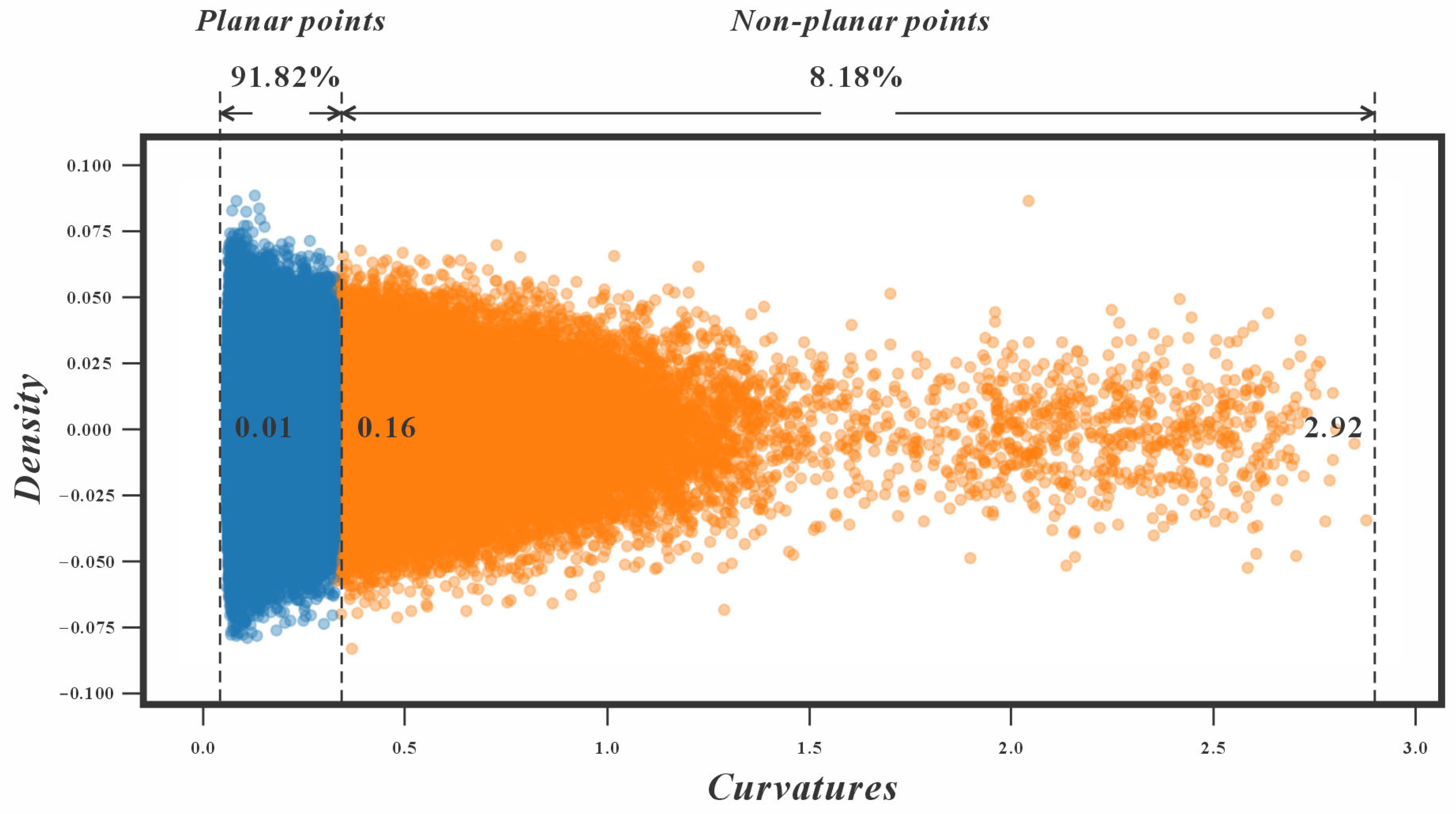
22]. For curvature thresholding, we first analyze the curvature distribution and apply K-means++ clustering (k = 2) to separate non-planar points (higher curvature) from planar points (lower curvature). The first cluster (lower curvature, 0.01–0.16) was classified as planar points, while the second (higher curvature) was classified as non-planar points. Thus, the curvature distribution after clustering (
Figure 6) justifies this threshold range: 0.01–0.16 (the dataset comprises 91.82% planar points and 8.18% non-planar points).
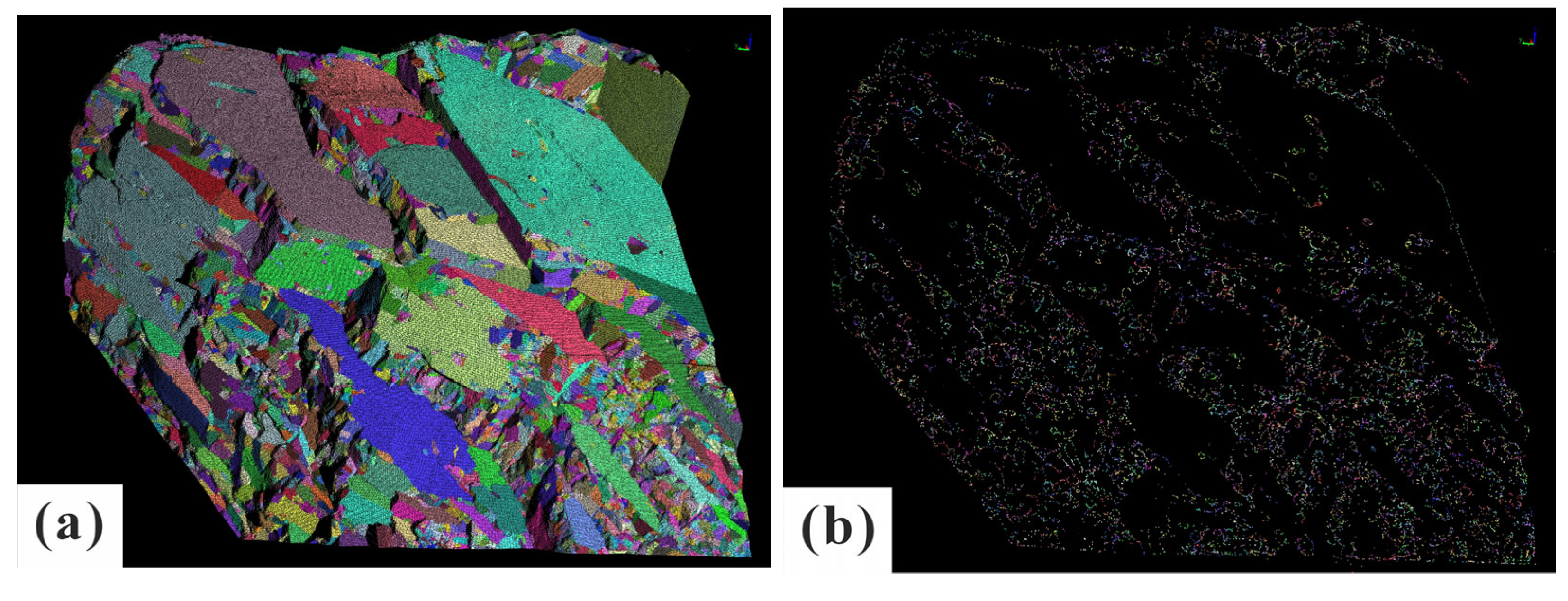
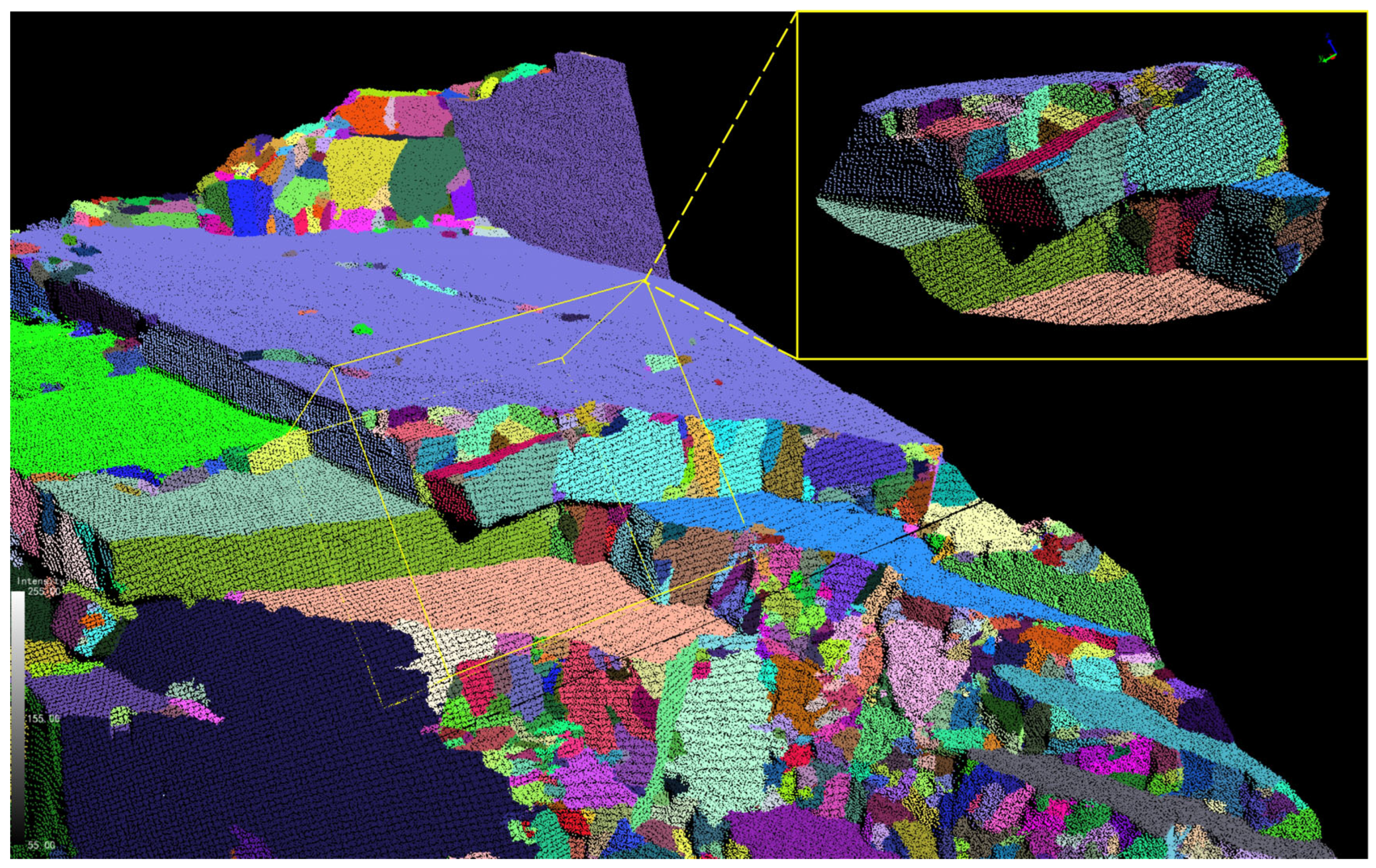
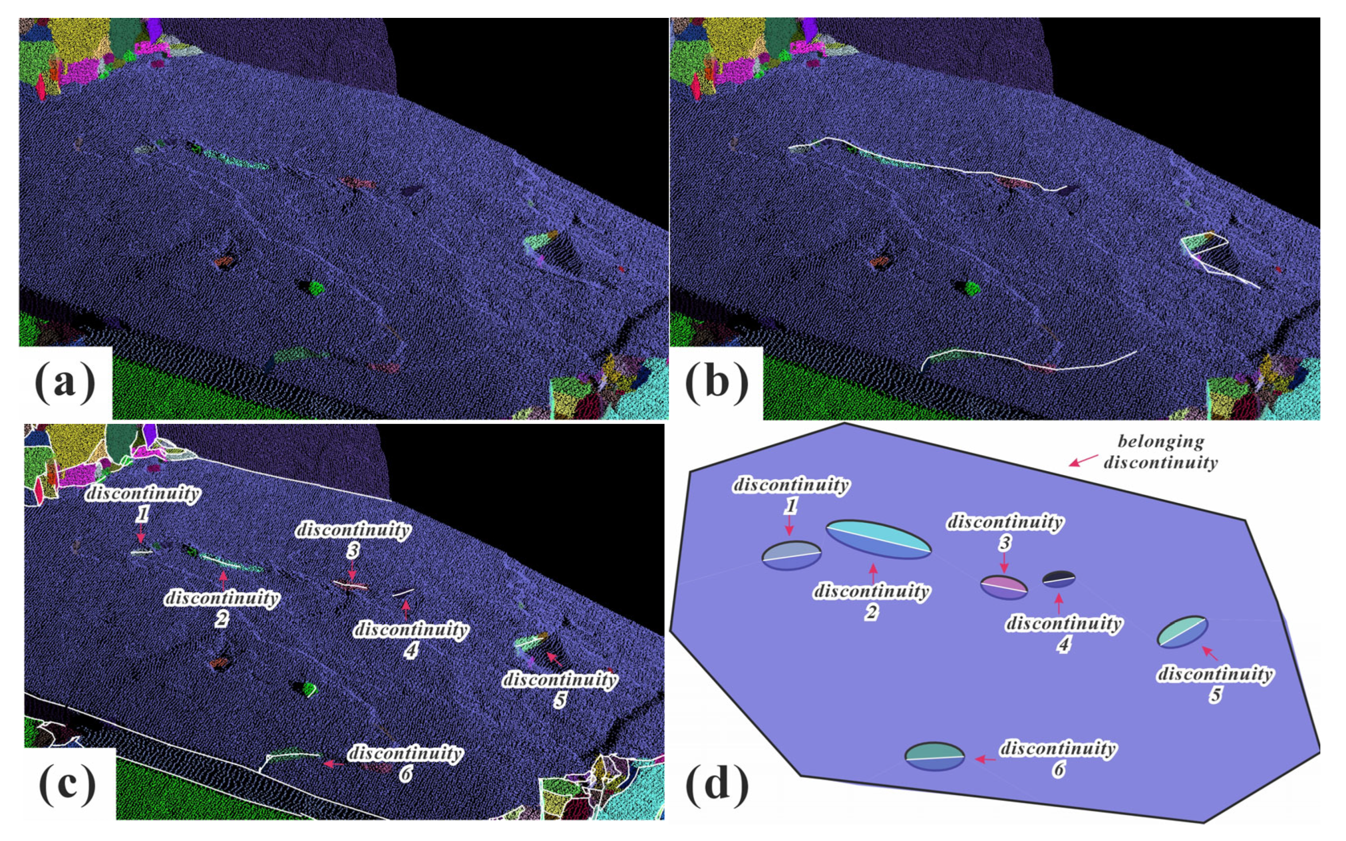
For comparative evaluation, we selected the conventional region-growing algorithm for discontinuity segmentation (noting that ARCG performs both discontinuity and boundary extraction simultaneously, though it can execute discontinuity segmentation alone if boundary extraction is disabled). We also employed the widely used alpha-shape algorithm for boundary point extraction. Both methods were systematically compared with our proposed approach. As illustrated in
Figure 7, the conventional region-growing algorithm requires iterative parameter tuning, frequently leading to under-segmentation or over-segmentation of discontinuities. This necessitates additional post-processing steps such as re-segmentation or merging operations. Similarly, the alpha shape algorithm demands repeated parameter adjustments to identify optimal values. In contrast, our method dynamically adapts thresholds to local conditions while simultaneously extracting boundary points, achieving both precision and computational efficiency in automated extraction.
