Highlights
What are the main findings?
- The proposed Optical Flow Method (OFM) achieves sub-pixel accuracy and a 30-fold increase in computational efficiency for monitoring large-gradient mining displacements, compared to Pixel Offset Tracking (POT).
What are the implications of the main findings?
- The OFM provides a reliable and efficient tool for large-gradient displacement monitoring, offering critical technical support for mining-induced hazard assessment and risk management.
Abstract
Monitoring large-gradient surface displacement caused by underground mining remains a significant challenge for conventional Synthetic Aperture Radar (SAR)-based techniques. This study introduces optical flow methods to monitor large-gradient displacement in mining areas and conducts a comprehensive comparison with Small Baseline Subset Interferometric SAR (SBAS-InSAR) and Pixel Offset Tracking (POT) methods. Using 12 high-resolution TerraSAR-X (TSX) SAR images over the Daliuta mining area in Yulin, China, we evaluate the performance of each method in terms of sensitivity to displacement gradients, computational efficiency, and monitoring accuracy. Results indicate that SBAS-InSAR is only capable of detecting displacement at the decimeter level in the Dalinta mining area and is unable to monitor rapid, large-gradient displacement exceeding the meter scale. While POT can detect meter-scale displacements, it suffers from low efficiency and low precision. In contrast, the proposed optical flow method (OFM) achieves sub-pixel accuracy with root mean square errors of 0.17 m (compared to 0.26 m for POT) when validated against Global Navigation Satellite System (GNSS) data while improving computational efficiency by nearly 30 times compared to POT. Furthermore, based on the optical flow results, mining parameters and three-dimensional (3D) displacement fields were successfully inverted, revealing maximum vertical subsidence exceeding 4.4 m and horizontal displacement over 1.5 m. These findings demonstrate that the OFM is a reliable and efficient tool for large-gradient displacement monitoring in mining areas, offering valuable support for hazard assessment and mining management.
1. Introduction
The exploitation of mineral resources, especially underground mining, is a key driver of large-gradient ground displacements like subsidence and fissures, thereby posing a significant threat to mining safety, ecological balance, and infrastructure stability [1,2]. Frequent underground mining activities are highly likely to trigger geological disasters such as surface subsidence, landslides, and ground collapses, which severely hinder the sustainable development of mining areas [3,4]. Therefore, establishing an efficient and high-precision displacement monitoring method in mining areas holds great scientific value and engineering significance [5]. It is crucial for early disaster warning, mining process optimization, and ecological restoration.
Currently, displacement monitoring in mining areas primarily depends on technologies such as the Global Navigation Satellite System (GNSS), leveling measurement, and Interferometric Synthetic Aperture Radar (InSAR) [5]. Among them, InSAR has emerged as the dominant method for displacement monitoring in mining areas due to its all-weather operation, wide coverage, and high spatial resolution [6]. However, InSAR technology encounters challenges in monitoring large-gradient displacement, as significant phase gradient can complicate or even prevent successful phase unwrapping, resulting in inaccurate measurements [7]. Research indicates that when the displacement gradient surpasses 1/4 of the radar wavelength cycle (e.g., approximately 1.4 cm in the C-band), phase unwrapping algorithms are prone to failure [8]. Phase unwrapping errors make it difficult to accurately acquire mining-induced large-gradient displacement fields. In addition, vegetation changes and other disturbances can lead to incoherent signals. This further restricts InSAR’s ability to continuously monitor complete displacement fields.
To address the limitations of phase-based methods, pixel offset tracking (POT) techniques have been developed to leverage SAR amplitude information [4,9]. These methods estimate surface displacement by tracking geometric offsets in the range and azimuth directions. POT methods such as COSI-Corr [10], Micmac [11], and QPEC/Medicis [12] have been developed and extensively applied in displacement monitoring, including seismic fault offsets [13], glacier flow velocities [14], landslides [15], and dune migration [16]. However, existing research indicates that these methods encounter significant challenges in computational efficiency and in accurately monitoring displacement. Firstly, the offset calculation requires performing cross-correlation operations across the entire image, leading to computational complexity that grows exponentially with the monitoring area expansion [17]. For instance, processing a single Sentinel-1 image to solve the offset can take several hours, which is not conducive to the high-frequency and near-real-time monitoring demands of mining areas. Moreover, the accuracy of these methods is greatly influenced by image registration errors and terrain residuals [18,19].
In recent years, the Optical Flow method (OFM) [20,21], a computer vision technique based on continuous motion field modeling in the space-time domain, has offered new ideas for monitoring large-gradient displacement in mining areas. Its core advantages are as follows: (1) By establishing pixel motion continuity constraints between neighboring images, the algorithm can effectively solve large-gradient displacement fields. (2) It uses variational optimization or a deep learning framework to achieve sub-pixel displacement estimation, theoretically improving accuracy by approximately 30–50% compared to traditional POT techniques. (3) Its computational efficiency is significantly enhanced, with the OFM processing a single scene image in just a few minutes. Since the 1980s, the OFM has been applied in fields such as earthquakes [22], glacial movements [23], and landslide monitoring [24]. The results are of the same order of magnitude as and denser than those of the POT method. However, there have been relatively few studies on applying the OFM to mining displacement monitoring.
In this study, we collected 12 scenes of high-resolution TerraSAR-X (TSX) SAR data with 11-day intervals. Then, we used SBAS-InSAR, POT, and OFM to obtain mining-induced subsidence displacement time series and compared the results of the three methods. Finally, we selected the OFM displacement monitoring results to invert the mining parameters and three-dimensional displacement of the mining area.
2. Study Area and Data
2.1. Study Area
In this study, we focus on the Daliuta mining area in Yulin City, Shaanxi Province, China (Figure 1). As a typical mining area in the Loess Plateau, it has distinct geographic features and faces serious ecological challenges. The geology of the Dalinta area comprises a stratigraphic sequence from the Triassic Yongping Formation (T3y) to the Quaternary System (Q), including the Jurassic Fuxian (J1f), Yan’an (J1-2y), Zhiluo (J2z), and Anding (J2a) Formations [25]. Climatically, the region falls within the northern temperate semi-arid continental monsoon zone, with aridity, low rainfall, and high evaporation; the mean annual evaporation is about 2049.6 mm, representing a volume 4–5 times that of the annual precipitation [26]. As a key national coal mine production area, the mining lies in an arid zone. This creates a dual ecological pressure from extreme water scarcity and intensive mining. Mining has produced geological displacement—such as crack networks and collapse pits (Figure 1) [27]—and has triggered secondary hazards, including induced seismicity and landslides. Consequently, the inherently fragile semi-arid ecosystem is experiencing accelerated degradation.
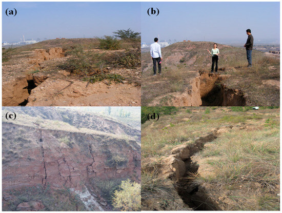
Figure 1.
Photographs documenting ground fissures and collapse pits induced by coal mining activities, taken in 2013. The location where the photograph was taken is shown in the yellow box in Figure 2c. (a,d) ground fissures; (b,c) collapse pits.
This study focuses on the 52304 coal mining face (marked by the black rectangle in Figure 2b), which was mechanized from 1 November 2011 to 25 March 2013. In Figure 2c, the black lines represent the positions of the longwall faces with their corresponding dates, and the white lines indicate the coal mine roadways. The surface elevation of the mining area ranges from 1154.8 m to 1269.9 m, with a vertical mining depth of 230 m [27,28]. The average thickness of the main coal seam is 6.94 m, dipping gently at 1–3°. Global Navigation Satellite System (GNSS) monitoring revealed that mining activities between 13 December 2012 and 11 March 2013 induced a vertical subsidence of 4.4 m, resulting in typical mining-induced surface features such as radial ground fractures and a butterfly-shaped subsidence basin [27,28]. The longwall fully mechanized top coal caving mining method was employed, with an average daily advance rate of 3.86 m/day and an extraction ratio of 0.646 [27]. The goaf was managed using the so-called ceiling collapse method to mitigate surface subsidence and ensure surrounding rock stability.
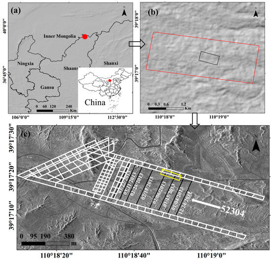
Figure 2.
Location of the study area and coverage of SAR images. (a) Location of the study area in China and Shaanxi Province. (b) The working face of the mining (black box) and the coverage of SAR images (red box). The red dot indicates the location of the study area. (c) Amplitude image of a mine roadway from TSX. White lines indicate the coal mine roadways, while black lines mark the positions of the longwall faces with their corresponding dates. The yellow box denotes the photographic position for Figure 1.
2.2. Datasets
To monitor the displacement evolution of the 52304 working face, we collected 12-view TSX data from November 2012 to April 2013. The data has an 11-day repeat cycle with 0.91 m range resolution and 0.86 m azimuth resolution. Using the SBAS strategy with a 40 day temporal-baseline threshold, 30 interferometric pairs were generated (Figure 3). A 30 m SRTM DEM was incorporated for the topographic phase of InSAR removal.
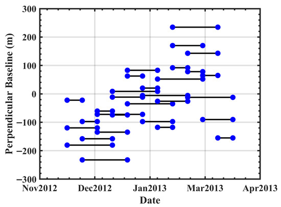
Figure 3.
Spatiotemporal-baseline map, where the blue dots indicate the acquisition time of the SAR images and the black lines indicate the image pairs.
3. Method
In this section, we first aligned the acquired TSX SAR data and generated multiple master–slave image pairs according to the SBAS strategy, as illustrated in Figure 4. We then applied SBAS-InSAR, POT, and OFM to derive the mining’s displacement time series, followed by a comparative analysis of the advantages and limitations of each method. Finally, using the Line-of-Sight (LOS) displacement results, we inverted the mining parameters and reconstructed the three-dimensional (3D) displacement time series of the mining area.
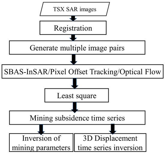
Figure 4.
Flowchart of data processing.
3.1. SBAS-InSAR Method
SBAS-InSAR generates interferometric pairs by setting short temporal and spatial baseline thresholds. This approach minimizes the effects of temporal and spatial incoherence, improves interferogram coherence, and enhances the accuracy and reliability of displacement measurements. During processing, one Single Look Complex (SLC) image is chosen as the reference master. The remaining SLC images are co-registered to this master image. Temporal and spatial baseline thresholds are then applied to generate interferometric pairs. These pairs are combined with external digital elevation model (DEM) data for differential interferometric processing. Finally, phase filtering, phase unwrapping, and error correction are applied to the resulting differential interferograms.
The following observation equations can be formulated for the wrapped differential interferometric phase [29]:
where and represent the deformation at times and , respectively, relative to the initial SAR data acquisition time . denotes the corresponding unwrapped phase value of the -th interferogram, and indicates the number of interferograms. Equation (1) is a set of equations containing several unknowns, which can be written in matrix form as follows:
where is the design matrix corresponding to the multiple interferograms. Equation (2), is the design matrix. Equation (2) can be estimated using the least squares criterion:
where represents the inverted displacement time series. When divided into several small baseline subsets, the columns of the design matrix fail to satisfy the rank condition, resulting in an infinite number of least squares solutions for Equation (3). To address this, we introduce the least squares criterion and apply singular value decomposition (SVD) to the design matrix to obtain the optimal least squares solution for the estimated parameter.
3.2. Pixel Offset Tracking Method
SAR images have a limited bandwidth, which causes phase-based InSAR techniques to struggle with large-gradient displacements and makes it difficult to reliably monitor surface displacement. However, the SAR offset tracking technique, which relies on SAR image intensity information, can effectively monitor large-gradient displacements. The accuracy of this technique depends on the resolution of the images. As demonstrated by Leprince et al. [30], the theoretical accuracy of the POT technique is limited by the sub-pixel interpolation algorithm, and it can typically reach 1/20 of a pixel under ideal conditions. However, the practical accuracy is severely affected by image texture and signal-to-noise ratio. Low-resolution images exacerbate the loss of texture information, leading to an increase in mismatches of correlation peaks. Additionally, excessively low resolution fails to meet the Nyquist criterion for spatial sampling, which reduces the accuracy of displacement inversion. By calculating offsets using a mutual correlation algorithm, this method can monitor surface changes in both the LOS and azimuthal directions.
The basic principle of SAR POT is to use the coherence of two SAR images to measure surface displacement. When a surface target moves between two observations, coherence decreases. Analyzing the differences between the two images yields pixel displacement information. The workflow is as follows: First, both master and slave images are co- and fine-registered using intensity data and precise orbit information to ensure pixel-to-pixel correspondence. Next, within a reference window on the master image, a search window of identical size is defined on the slave image. A normalized cross-correlation metric is then computed across the search window to identify the displacement that maximizes similarity, yielding sub-pixel estimates of surface movement. Finally, the point-by-point correlation number is calculated using Equation (4) [31].
where denotes the normalized inter-correlation index; the size of the SAR image is ; the coordinates of the computed pixels in the image are ; and denote the intensity values at the same location between the master and slave images; and and denote the intensity averages within the window of the master and slave images. An image block A of size is selected in the master image, and a corresponding image block B of the same size () is selected within the search window on the slave image. According to Equation (4), the number of correlations between image blocks A and B is calculated. The displacement (offset) is determined when the normalized correlation index reaches its maximum value.
3.3. Optical Flow Method
Optical flow refers to the instantaneous velocity field of a moving object as observed through a sequence of images. As the object moves, its position in the observation plane shifts, and the rate of this movement at any given moment is termed optical flow [32]. This velocity field is derived from the apparent motion of image features between consecutive frames, providing information about the direction and speed of motion within the scene. There is a point on the imaging plane, and the gray value at a certain moment is . After a period of time , this point moves to a new position, and the position coordinates of the point at this time are . The gray value of this point becomes . According to the assumption of image consistency in the two basic assumptions of the OFM, the luminance of the points on the image before and after the movement is unchanged, and thus we can obtain . Let be the optical flow vector at point . The Taylor expansion of the shifted gray values is . Ignoring the terms higher than the second order, the optical flow equation is obtained as follows [20,21]:
where is a tiny amount of time, the above equation can be deformed as:
where the optical flow field components between two neighboring images are
The two components are also the velocity components of the optical flow vectors in the and directions at the point . The pre-movement light intensity is obtained by taking the partial derivatives of as and , respectively, whose values can be obtained by estimating the first-order difference in the neighboring image target pixel points in the image sequence. Equation (6) is the fundamental optical flow equation. To solve for the velocity components, additional constraints are required. This study adopts the GeFolki algorithm (https://github.com/aplyer/gefolki (accessed on 10 May 2025)) [23,33], which is well suited for heterogeneous remote sensing image alignment and is robust to grayscale variations. The algorithm utilizes an image pyramid strategy to optimize optical flow computation. In each pyramid layer, a ranking function first sorts the pixel grayscale values within a local region, compressing the grayscale range to enhance the image. The optimal displacement is then approximated through least squares estimation, using the Gaussian Newton iterative method with an accurate Taylor expansion. During the iterative process, the window radius is gradually reduced from large to small, refining the displacement estimates. For pyramid processing, a Gaussian pyramid is constructed for each image. The upper pyramid layers have lower resolution, while the lower layers have higher resolution. If the target displacement in the original image is denoted as , the displacement in the -th layer is calculated as follows [23,33]:
where represents the number of layers in the pyramid image. Reflecting the result of the optical flow in the top layer to the sub-top layer and using it as the optical flow estimate g for that layer, the optical flow in the sub-top layer can be expressed as:
In each layer of the image, the optical flow of that layer is obtained by minimizing the objective Equation (9), and the target displacement d of the bottom layer of the pyramid can be obtained by iterating sequentially:
Stable estimation of the target pixel point displacement is achieved by accumulating the optical flow results from different layers of the pyramid in layers from coarse to fine.
4. Results
4.1. SBAS-InSAR Results
Firstly, 12 TSX Spotlight mode SAR images acquired between 10 November 2012 and 2 April 2013 were processed based on the SBAS-InSAR technology. To effectively monitor the surface displacement characteristics induced by mining, the full-resolution data processing strategy was first adopted to generate differential interferograms, and the decorrelation noise was effectively suppressed by the Goldstein filtering method, followed by the phase unwrapping using the minimum cost flow (MCF) algorithm. A coherence coefficient threshold of 0.5 was set to mask the low coherence region to eliminate the influence of phase unwrapping errors. According to the engineering records of the mining area, the mining operation at the target working face was completed on 25 March 2013. This provided a crucial reference point for analyzing the displacement time series and assessing the impact of mining activities on surface displacement over time. The SBAS-InSAR displacement time series results are presented in Figure 5. The results demonstrate that the InSAR technique has significant limitations in monitoring the mining area due to large-gradient displacement caused by mining activities. Underground resource extraction often triggers large-gradient surface displacement (exceeding meter-scale) within a short period (ranging from days to weeks). As a result, the displacement gradient surpasses the maximum phase gradient detectable by X-band radar systems, leading to challenges in accurately capturing and analyzing the displacement. This phenomenon leads to severe aliasing of radar interferometric phases, rendering conventional phase unwrapping algorithms ineffective. Consequently, the SBAS-InSAR technique was only able to detect small displacement signals in the fringe areas of the mining. Monitoring data indicate that the maximum cumulative displacement between November 2012 and April 2013 was 242 mm, which is significantly less than the maximum actual displacement of 4.4 m observed during the mining process. The precision of the displacement estimates, evaluated through the error propagation law based on a 4.93 mm standard deviation in stable areas based on displacement time series, is presented in Figure 6a. The final epoch exhibits uncertainty of 5.30 mm (Figure 6b). These results are consistent with the findings of Fan et al. [27], who reported a maximum cumulative displacement of 202 mm in the same mining area during the same period using InSAR technology. Theoretical analysis reveals that when the displacement gradient exceeds the critical value corresponding to the radar wavelength, the phase difference between neighboring image pixels will surpass π radians, resulting in phase unwrapping errors, commonly known as “phase jumps”. It is noteworthy that despite using TSX data with an 11-day revisit cycle and 1 m resolution, the interferometric phase still suffered from incoherence due to large-gradient displacements, rendering InSAR technology incapable of capturing the displacement in the central mining area. Therefore, SAR intensity information will be utilized to effectively capture large-gradient displacements in the mining areas.
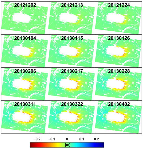
Figure 5.
Displacement time series in the LOS direction of mining working face 52304 were acquired by SBAS-InSAR. The data represent cumulative displacement relative to the start of mining activities in November 2012, with each subplot titled in the format “YYYYMMDD”.
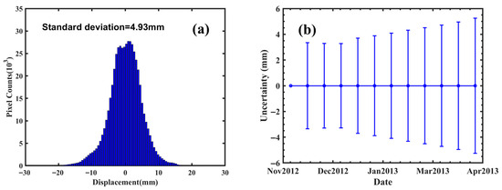
Figure 6.
(a) Displacement time series histogram from stable area (all areas with the exception of the mining working face). (b) Displacement time series uncertainty from the error propagation law of the baseline network (Figure 3).
4.2. POT and OFM Results
Figure 7a–c show the LOS results from the POT method at different window sizes, while Figure 7d presents the results from the optical flow method. The displacement results indicate that the POT method can capture larger magnitudes of displacement when using a smaller window size (e.g., 32 × 32). However, significant mismatches are observed, introducing substantial noise into the results. As the window size increases (from 32 × 32 to 64 × 64 and 128 × 128), the noise in the results gradually decreases. However, this also leads to a reduction in the detected magnitude of displacement within the mining subsidence zone. In contrast, the OFM combines the accuracy of small-window POT configurations with the reliability of large-window approaches. During iterative solving, the OFM dynamically adjusts the window size (from 49 × 49 → 41 × 41 → 33 × 33 → … → 9 × 9). The process begins with a large radius to ensure a smooth and reliable estimation and then gradually reduces the radius to achieve an optimal result, thereby capturing higher-resolution details.
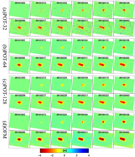
Figure 7.
The LOS displacement time series maps obtained by POT and OFM. (a–c) The POT results with windows 32, 64, and 128, respectively. (d) OFM result. The data represent cumulative displacement relative to the start of mining activities in November 2012, with each subplot titled in the format “YYYYMMDD”.
Both the POT method and the OFM are capable of detecting displacement exceeding 3 m in the subsidence center of the mining area compared to InSAR results. We calculated the average cumulative displacement over the mining panel, which measured −1.32 m (32 × 32), −1.71 m (64 × 64), and −1.57 m (128 × 128) using the POT method, and −2.12 m using the OFM. This indicates that the OFM detects a greater magnitude of displacement in the mining area than the POT method. Furthermore, for a SAR image of 2100 × 1500 pixels, the processing time required by the OFM is 21 s, compared to 168 s (32 × 32), 621 s (64 × 64), and 2641 s (128 × 128) for the POT method—corresponding to speedup factors of 8, 30, and 131, respectively. Thus, the OFM demonstrates significantly higher computational efficiency than the POT method.
Figure 8 shows the displacement time series at three representative points obtained using different methods. Among them, P1 point is the first to undergo displacement due to mining activities, followed by P2 and P3. The results indicate that the POT method with a 32 × 32 window (blue line) produces a time series with strong fluctuations. Notably, the P3 point, which is expected to subside, exhibits uplift instead, completely failing to capture the temporal evolution of mining-induced displacement. As the POT window size (64 × 64, 128 × 128) increases (green and pink lines), these fluctuations gradually decrease, and P3 correctly indicates subsidence. However, the maximum subsidence magnitude at P1 decreases. In contrast, the displacement time series obtained by OFM not only exhibits a larger magnitude but also demonstrates significantly reduced fluctuation. Moreover, its temporal variation closely follows the typical “S-shaped curve” (characterized by a “slow–fast–slow” displacement pattern) associated with complete mining activity, demonstrating better consistency with the actual mining process. The mining timeline was integrated with the OFM displacement time series, as shown in Figure 9. It can be observed that as mining advances along the working face, both the spatial extent and magnitude of ground displacement continue to increase.
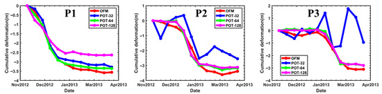
Figure 8.
The LOS displacement time series at three typical points P1~P3 (in Figure 10).
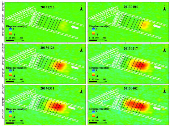
Figure 9.
Overview maps of mining face locations, mining timeline (Figure 2c), and OFM displacement time series. White lines indicate the coal mine roadways, while black lines mark the positions of the longwall faces with their corresponding dates.
To quantify the discrepancies between the OFM results and the POT results obtained with different window sizes, we generated scatter correlation plots, discrepancy maps, and statistical histograms of the cumulative LOS displacement, as shown in Figure 10 and Figure 11. The results indicate that the POT method with a 32 × 32 window exhibits considerable deviation from the OFM results, with a correlation coefficient of only 0.67 and a root mean square error (RMSE) of 0.67 m. In comparison, the POT method with a 64 × 64 window shows a higher correlation of 0.9 with the OFM results, along with a lower RMSE of 0.26 m. The highest correlation is achieved by the POT method with a 128 × 128 window, reaching 0.93, while also yielding the smallest RMSE of 0.23 m. However, the slope of the linear fit for the 128 × 128 POT results is 0.75, which is lower than that of the 64 × 64 window results (0.83). These findings indicate that while parameter settings—particularly window size—significantly influence the POT method’s performance in mining displacement monitoring, POT and OFM demonstrate high consistency in monitoring results at the Daliuta mining area.
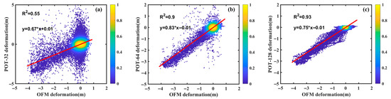
Figure 10.
Cross-correlation between cumulative displacement derived from the OFM and POT methods with various window sizes: (a) 32 × 32, (b) 64 × 64, (c) 128 × 128.
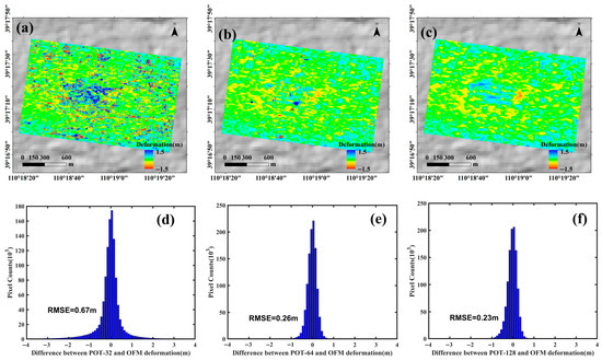
Figure 11.
Discrepancies in cumulative displacement between the OFM and POT methods with different window sizes and their respective statistical histograms: (a,d) 32 × 32, (b,e) 64 × 64, (c,f) 128 × 128.
4.3. Comparison with GNSS Results
Figure 12 illustrates the distribution of 62 GNSS monitoring points across the mining working face, spaced at 25 m intervals. The GNSS data, along with displacement monitoring results from different methods, are qualitatively compared against the averaged displacement estimates derived from both the OFM and the POT method within a 20 m radius of each GNSS point. The GPS measurement period spanned from 13 December 2012 to 3 April 2013, covering the entire primary mining cycle. The GNSS reference data were obtained from the study by Fan et al. [27] and were used for comparative analysis with the OFM and POT results during the period from 13 December 2012 to 3 April 2013.
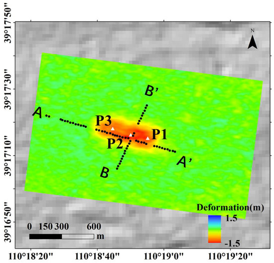
Figure 12.
Temporal and spatial locations of GNSS points and P1~P3 points, with the cumulative displacement solved by the OFM in the background. AA’ and BB’ denote GNSS positions.
Figure 13 compares the LOS displacement results along strike AA′ and dip BB′. For a window size of 32 × 32, the RMSEs between the POT result and GNSS data are 0.91 m (AA′) and 0.83 m (BB′), with a mean value of 0.87 m. When the window size is increased to 64 × 64, the RMSEs decrease to 0.30 m and 0.23 m, respectively, yielding a mean of 0.27 m. Further increasing the window size to 128 × 128 reduces the RMSEs to 0.27 m and 0.24 m, with a mean value of 0.26 m. In contrast, the OFM achieves lower RMSEs of 0.23 m (AA′) and 0.11 m (BB′), corresponding to a mean of 0.17 m, demonstrating superior accuracy and computational efficiency compared to the POT method.
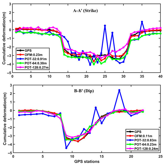
Figure 13.
Verification of accuracy of optical flow LOS displacement results and pixel offset LOS displacement results using GNSS points [27].
5. Discussion
5.1. Performance Comparison of InSAR, POT, and OFM in Mining Displacement Monitoring
This study presents a comprehensive evaluation of the performance of SBAS-InSAR, POT, and the OFM in monitoring large-gradient mining-induced surface displacement (Table 1). The results indicate that while each technique has its distinct advantages, OFM achieves a superior balance among computational efficiency, spatial resolution, and accuracy under high-displacement-gradient conditions. In mining displacement monitoring, conventional SBAS-InSAR—reliant on phase unwrapping—proves incapable of effectively capturing meter-scale subsidence. Although POT overcomes gradient limitations by utilizing SAR intensity information, its computational demands remain a constraint for large-area or near-real-time applications. Experiments show that over the same coverage area, POT requires approximately 8 to 131 times longer processing time than OFM. Moreover, its accuracy is highly sensitive to window size selection: smaller windows introduce noise, while larger ones sacrifice detail.

Table 1.
Performance comparison of InSAR, POT and OFM in mining-induced displacement monitoring.
In contrast, the OFM employed in this study incorporates a multi-scale pyramid optimization strategy, enabling efficient and robust estimation of sub-pixel displacements while preserving spatial detail. When validated against GNSS data, OFM outperformed all POT configurations with varying window sizes. Furthermore, the integration of line-of-sight displacement derived from OFM with the Probability Integral Method (PIM) and 3D displacement inversion techniques underscores its practical utility in retrieving mining parameters and reconstructing complex displacement dynamics. This approach successfully captured the temporal evolution of subsidence and horizontal displacement, showing strong consistency with independent ground measurements and mining records.
5.2. PIM Inversion of Mining Parameters
Based on previous studies [5,28,36,37], we utilize the cumulative displacement results derived from the OFM and apply a Bayesian inversion framework to estimate mining-related parameters. The core inversion model is the PIM, which is grounded in the theory of random media. In this model, the overburden is considered an idealized, loose, random medium composed of numerous infinitesimal units. Underground mining activities are treated as random events that induce surface subsidence. The resulting surface displacement is modeled as the cumulative effect of subsidence caused by the extraction of these individual units. This method has been widely adopted for predicting surface subsidence in Chinese coal mining areas, demonstrating both strong theoretical foundations and practical effectiveness.
The governing equations are given in Equations (11)–(13), where the vertical and horizontal (strike and dip) displacements at any surface point (x, y) can be expressed as follows:
where
where is the mining thickness; is the subsidence coefficient; is the dip angle; , and are the mining depths of the seams; is the tangent of the main influence angle; and are the strike and tendency lengths of the working face, respectively; ~ are the left, upper, right and lower deviations of the inflection point, respectively; is the propagation angle of the mining influence, which is approximately equal to the maximum subsidence angle ; b is the displacement factor; erf (x) is the error function; and are the horizontal angles between the counterclockwise rotation of the x-axis in the mine coordinate system and the geographic north and east directions, respectively; and , , and are the horizontal displacements in the surface subsidence and north–south and east–west directions, respectively.
Based on the above method to invert the parameters of the PIM, according to the a priori information such as the mining report and geological conditions of the mining, we set the main parameters as follows: = 0.65, = 0.3, = 2.2, = 87, = = = = 20. Based on the set model parameters and their initial upper and lower bounds and step sizes, we perform the parameter inversion through the above model to obtain the optimal solution. In the process of parameter inversion, we adopt the optimization strategy based on residual minimization. By comparing the residuals between the original displacement field and the simulated displacement field, the inversion steps are dynamically adjusted to improve the parameter optimization effect. To further improve the stability and accuracy of the inversion, we introduce an adaptive step-size adjustment mechanism. This mechanism dynamically adjusts the step size of the parameter update according to the trend of the residual difference in each iteration so as to avoid falling into the local optimal solution and accelerate the convergence speed. The inversion results are shown in Figure 14, where (a) is the displacement result of the original observation, (b) is the simulation result based on the model, and (c) is the residual plot between the two. The standard deviation of the residuals is 0.24 m. In addition, Table 2 demonstrates the values of the parameters obtained from the inversion, which further validates the validity and reliability of the model. In the study area, our inversion results are closer to actual measurements than the mining parameters previously derived by Fan et al. [27].
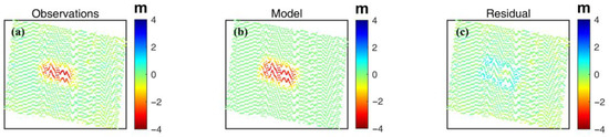
Figure 14.
Inversion results of mine parameters: (a) observed values; (b) modeled values; (c) residuals.
Table 2.
Inversion results and errors of underground mining area characteristics.
5.3. Three-Dimensional Displacement Inversion of the Mining
We applied the SGI method proposed by Yang et al. [32,33,38] to derive the 3D surface displacement time series associated with mining activities. This method establishes proportional relationships between vertical displacement gradients and horizontal displacements (north–south and east–west) in the mining area. These relationships are constrained by key mining parameters, including the main influence angle of mining ( = 2.2), the mining depth ( = 230 m), and the horizontal movement coefficient ( = 0.3). Using these constraints, two additional equations are incorporated into the inversion framework. Consequently, the LOS displacement from November 2012 to April 2013 obtained by the OFM can be used directly to first invert the vertical displacement (UD) and then to estimate the east–west (EW) and north–south (NS) components. The resulting 3D displacement field is shown in Figure 15.
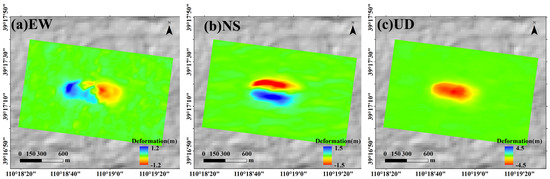
Figure 15.
Three-dimensional displacement of the mining area. (a–c) They are the north–south, east–west, and vertical displacements, respectively. (a) EW, (b) NS, (c) UD.
The results indicate that after the completion of underground mining in the 52304 working face, the maximum vertical subsidence reached 4.44 m; the maximum horizontal displacements were 1.21 m East, 0.95 m West, 1.52 m North, and 1.45 m South. To validate the accuracy of the 3D displacement inversion, we collected cumulative GPS measurements in profile BB’ of vertical and horizontal displacement from 21 November 2012 to 1 April 2013—a period nearly identical to the TSX data observation timeframe (November 2012 to April 2013). Figure 16 compares the GNSS-derived vertical and horizontal measurements with the 3D displacement results inverted using the SGI method, showing good agreement between the two. The RMSEs in the vertical and horizontal directions are approximately 0.1 m and 0.07 m, respectively. These errors account for only 2.2% and 4.6% of the maximum field-measured values in the vertical (about 4.45 m) and horizontal (around 1.52 m) directions, respectively. This accuracy meets the practical requirements for mining-induced displacement monitoring [39] (i.e., errors less than 10% and 20% in the vertical and horizontal directions, respectively). Compared with existing studies in the region, the inversion accuracy of our 3D displacement results is slightly better than that reported by Yang et al. [38], who obtained RMSEs of approximately 0.22 m and 0.11 m in the vertical and horizontal directions, respectively. Moreover, the horizontal accuracy achieved in this study is comparable to that reported by Chen et al. [40].
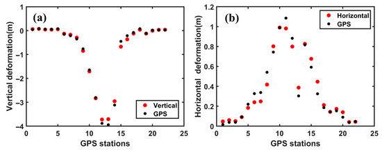
Figure 16.
Comparison between GPS measurements and the estimated 3D displacement in profile BB’. (a) Vertical direction; (b) Horizontal direction.
6. Conclusions
This study compares the performance of SBAS-InSAR, POT, and OFM for monitoring surface displacement in mining areas. The results demonstrate that the OFM offers significant advantages in detecting large-gradient displacements. Experimental analyses show that, by employing a multi-scale pyramid optimization strategy, the OFM effectively overcomes the phase unwrapping challenges of traditional InSAR and the inefficiencies of the POT method. This approach achieves a balance between computational efficiency—processing a single image pair within tens of seconds—and sub-pixel accuracy, with 0.17 m RMSE values. Mining parameters inverted using Bayesian inference and the probability density integration method show good agreement with observed data. Furthermore, the SGI-derived 3D displacement field captures both vertical subsidence and horizontal displacement patterns, with a maximum vertical subsidence of 4.44 m, consistent with recorded mining activity. Overall, the OFM provides robust technical support for large-gradient displacement monitoring. However, its performance in complex terrain still requires further improvement. Future work may explore the integration of deep learning techniques to enhance algorithm robustness and the fusion of multi-source data to improve the accuracy of 3D displacement inversion.
Author Contributions
C.Z. and J.C. designed the experiments. C.Z. performed the experiments and produced the results. J.C. drafted the manuscript and finalized the manuscript. C.Z. and J.C. contributed to the discussion of the results. All authors have read and agreed to the published version of the manuscript.
Funding
This research received no external funding.
Data Availability Statement
The original contributions presented in this study are included in the article. Further inquiries can be directed to the corresponding author.
Acknowledgments
We are grateful to the NASA Jet Propulsion Laboratory for providing SRTM DEM data. During the preparation of this manuscript, the authors used DeepSeek (https://www.deepseek.com/) to polish the English writing for a more native-speaker style. The authors have reviewed and edited the output and take full responsibility for the content of this publication.
Conflicts of Interest
Author Chuanjiu Zhang was employed by the company Shendong Coal Group Co., Ltd. The remaining authors declare that the research was conducted in the absence of any commercial or financial relationships that could be construed as a potential conflict of interest.
References
- Peng, S.; Ma, W.; Zhong, W. Surface Subsidence Engineering; Society for Mining, Metallurgy, and Exploration, Inc.: Littleton, CO, USA, 1992. [Google Scholar]
- Brady, B.; Brown, E. Rock Mechanics for Underground Mining; Springer: Dordrecht, The Netherlands, 1985. [Google Scholar]
- Chen, H.; Zhao, C.; Li, B.; Gao, Y.; Chen, L.; Liu, D. Monitoring spatiotemporal evolution of Kaiyang landslides induced by phosphate mining using distributed scatterers InSAR technique. Landslides 2022, 20, 695–706. [Google Scholar] [CrossRef]
- Chen, L.; Zhao, C.; Li, B.; He, K.; Ren, C.; Liu, X.; Liu, D. Deformation monitoring and failure mode research of mining-induced Jianshanying landslide in karst mountain area, China with ALOS/PALSAR-2 images. Landslides 2021, 18, 2739–2750. [Google Scholar] [CrossRef]
- Yang, Z.; Li, Z.; Zhu, J.; Wang, Y.; Wu, L. Use of SAR/InSAR in Mining Deformation Monitoring, Parameter Inversion, and Forward Predictions: A Review. IEEE Geosci. Remote Sens. Mag. 2020, 8, 71–90. [Google Scholar] [CrossRef]
- Zhang, L.; Lu, Z. Advances in InSAR imaging and data processing. Remote Sens. 2022, 14, 4307. [Google Scholar] [CrossRef]
- Hanssen, R.F. Radar Interferometry: Data Interpretation and Error Analysis; Springer Science & Business Media: Berlin/Heidelberg, Germany, 2001; Volume 2. [Google Scholar]
- Rosen, P.; Hensley, S.; Joughin, I.; Li, F.; Madsen, S.; Rodriguez, E.; Goldstein, R. Synthetic aperture radar interferometry. Pro. IEEE 2000, 88, 333–382. [Google Scholar] [CrossRef]
- Wang, L.; Deng, K.; Zheng, M. Research on ground deformation monitoring method in mining areas using the probability integral model fusion D-InSAR, sub-band InSAR and offset-tracking. Int. J. Appl. Earth Obs. Geoinf. 2020, 85, 101981. [Google Scholar] [CrossRef]
- Leprince, S.; Ayoub, F.; Klinger, Y.; Avouac, J. Co-registration of optically sensed images and correlation (COSI-Corr): An operational methodology for ground deformation measurements. In Proceedings of the 2007 IEEE International Geoscience and Remote Sensing Symposium, Barcelona, Spain, 23–27 July 2007; pp. 1943–1946. [Google Scholar]
- Rosu, A.; Pierrot-Deseilligny, M.; Delorme, A.; Binet, R.; Klinger, Y. Measurement of ground displacement from optical satellite image correlation using the free open-source software MicMac. Isprs J. Photogramm. Remote Sens. 2015, 100, 48–59. [Google Scholar] [CrossRef]
- Cournet, M.; Giros, A.; Dumas, L.; Delvit, J.; Michel, J. 2D Sub-Pixel Disparity Measurement Using QPEC/Medicis. Int. Arch. Photogramm. Remote Sens. Spat. Inf. Sci. 2016, XLI-B1, 291–298. [Google Scholar]
- Ma, Z.; Li, C.; Jiang, Y.; Chen, Y.; Yin, X.; Aoki, Y.; Yun, S.; Wei, S. Space Geodetic Insights to the Dramatic Stress Rotation Induced by the February 2023 Turkey-Syria Earthquake Doublet. Geophys. Res. Lett. 2024, 51, e2023GL107788. [Google Scholar] [CrossRef]
- Li, J.; Li, Z.; Ding, X.; Wang, Q. Investigating mountain glacier motion with the method of SAR intensity-tracking: Removal of topographic effects and analysis of the dynamic patterns. Earth-Sci. Rev. 2014, 138, 179–195. [Google Scholar] [CrossRef]
- Liu, X.; Zhao, C.; Zhang, Q.; Lu, Z.; Li, Z. Deformation of the Baige landslide, Tibet, China, revealed through the integration of cross-platform ALOS/PALSAR-1 and ALOS/PALSAR-2 SAR observations. Geophys. Res. Lett. 2020, 47, e2019GL086142. [Google Scholar] [CrossRef]
- Mahmoud, A.; Novellino, A.; Hussain, E.; Marsh, S.; Psimoulis, P.; Smith, M. The use of SAR offset tracking for detecting sand dune movement in Sudan. Remote Sens. 2020, 12, 3410. [Google Scholar] [CrossRef]
- Cai, J.; Wang, C.; Mao, X.; Wang, Q. An Adaptive Offset Tracking Method with SAR Images for Landslide Displacement Monitoring. Remote Sens. 2017, 9, 830. [Google Scholar] [CrossRef]
- Li, M.; Zhang, L.; Dong, J.; Tang, M.; Xu, Q. Characterization of pre- and post-failure displacements of the Huangnibazi landslide in Li County with multi-source satellite observations. Eng. Geol. 2019, 257, 105140. [Google Scholar] [CrossRef]
- Jia, H.; Wang, Y.; Ge, D.; Deng, Y.; Wang, R. Improved offset tracking for predisaster deformation monitoring of the 2018 Jinsha River landslide (Tibet, China). Remote Sens. Environ. 2020, 247, 111899. [Google Scholar] [CrossRef]
- Adiv, G. Determining Three-Dimensional Motion and Structure from Optical Flow Generated by Several Moving Objects. IEEE Trans. Pattern Anal. Mach. Intell. 1985, 4, 384–401. [Google Scholar] [CrossRef]
- Chanut, M.; Gasc-Barbier, M.; Dubois, L.; Carotte, A. Automatic identification of continuous or non-continuous evolution of landslides and quantification of deformations. Landslides 2021, 18, 3101–3118. [Google Scholar] [CrossRef]
- Ding, M.; Chen, H.; Li, Z.; Liu, Z. Analysis of Surface Deformations on the Basis of Optical Flow Field Models from Optical Remote Sensing Images. Geomat. Inf. Sci. Wuhan Univ. 2024, 49, 1314–1329. [Google Scholar]
- Fu, Y.; Zhang, B.; Liu, G.; Zhang, R.; Liu, Q.; Ye, Y. An optical flow SBAS technique for glacier surface velocity extraction using SAR images. IEEE Geosci. Remote Sens. Lett. 2022, 19, 1–5. [Google Scholar] [CrossRef]
- Chen, H.; Zhao, C.; Tomás, R.; Reyes-Carmona, C.; Kang, Y. Integrating InSAR and non-rigid optical pixel offsets to explore the kinematic behaviors of the Lanuza complex landslide. Remote Sens. Environ. 2025, 320, 114651. [Google Scholar] [CrossRef]
- He, B.; Zhou, X. Study on Distribution Law of Three Overburden Zones in Shallow and Thick Coal Seam Mining of Daliuta Coal Mine. Coal Sci. Technol. 2022, 50, 1–6. [Google Scholar]
- Zhang, H.; Jiang, B.; Zhang, H.; Li, P.; Wu, M.; Hao, J.; Hu, Y. Hydrochemical characteristics and component sources of water in underground reservoirs in the Daliuta Coal Mine. Coal Geol. Explor. 2024, 52, 12. [Google Scholar]
- Fan, H.; Gao, X.; Yang, J.; Deng, K.; Yu, Y. Monitoring Mining Subsidence Using A Combination of Phase-Stacking and Offset-Tracking Methods. Remote Sens. 2015, 7, 9166–9183. [Google Scholar] [CrossRef]
- Fan, H.; Li, T.; Gao, Y.; Deng, K.; Wu, H. Characteristics inversion of underground goaf based on InSAR techniques and PIM. Int. J. Appl. Earth Obs. Geoinf. 2021, 103, 102526. [Google Scholar] [CrossRef]
- Berardino, P.; Fornaro, G.; Lanari, R.; Sansosti, E. A new algorithm for surface deformation monitoring based on small baseline differential SAR interferograms. IEEE Trans. Geosci. Remote Sens. 2002, 40, 2375–2383. [Google Scholar] [CrossRef]
- Leprince, S.; Barbot, S.; Ayoub, F.; Avouac, J. Automatic and precise orthorectification, coregistration, and subpixel correlation of satellite images, application to ground deformation measurements. IEEE Trans. Geosci. Remote Sens. 2007, 45, 1529–1558. [Google Scholar] [CrossRef]
- Sutton, M.; Wolters, W.; Peters, W.; Ranson, W.; Mcneill, S.R. Determination of displacements using an improved digital correlation method. Image Vis. Comput. 1983, 1, 133–139. [Google Scholar] [CrossRef]
- Horn, B.; Schunck, B. Determining optical flow. Artif. Intell. 1981, 17, 185–203. [Google Scholar] [CrossRef]
- Brigot, G.; Colin-Koeniguer, E.; Plyer, A.; Janez, F. Adaptation and Evaluation of an Optical Flow Method Applied to Coregistration of Forest Remote Sensing Images. IEEE J. Sel. Top. Appl. Earth Obs. Remote Sens. 2016, 9, 1–17. [Google Scholar] [CrossRef]
- Pan, B.; Qian, K.; Xie, H.; Asundi, A. Two-dimensional digital image correlation for in-plane displacement and strain measurement: A review. Meas. Sci. Technol. 2009, 20, 062001. [Google Scholar] [CrossRef]
- Barron, J.; Fleet, D.; Beauchemin, S. Performance of optical flow techniques. Int. J. Comput. Vis. 1994, 12, 43–77. [Google Scholar] [CrossRef]
- Yang, Z.; Xu, B.; Li, Z.; Wu, L.; Zhu, J. Prediction of mining-induced kinematic 3-D displacements from InSAR using a Weibull model and a Kalman filter. IEEE Trans. Geosci. Remote Sens. 2021, 60, 1–12. [Google Scholar] [CrossRef]
- Yang, Z.; Li, Z.; Zhu, J.; Hu, J.; Wang, Y.; Chen, G. InSAR-based model parameter estimation of probability integral method and its application for predicting mining-induced horizontal and vertical displacements. IEEE Trans. Geosci. Remote Sens. 2016, 54, 4818–4832. [Google Scholar] [CrossRef]
- Yang, Z.; Li, Z.; Zhu, J.; Preusse, A.; Hu, J.; Feng, G.; Papst, M. Time-series 3-D mining-induced large displacement modeling and robust estimation from a single-geometry SAR amplitude data set. IEEE Trans. Geosci. Remote Sens. 2018, 56, 3600–3610. [Google Scholar] [CrossRef]
- State Bureau of Coal Industry. Regulations of Coal Pillar Design and Extraction for Buildings, Water Bodies Railways, Main Shafts and Roadways; Coal e Press: Beijing, China, 2000. (In Chinese) [Google Scholar]
- Chen, B.; Li, Z.; Yu, C.; Fairbairn, D.; Kang, J.; Hu, J.; Liang, L. Three-dimensional time-varying large surface displacements in coal exploiting areas revealed through integration of SAR pixel offset measurements and mining subsidence model. Remote Sens. Environ. 2020, 240, 111663. [Google Scholar] [CrossRef]


Disclaimer/Publisher’s Note: The statements, opinions and data contained in all publications are solely those of the individual author(s) and contributor(s) and not of MDPI and/or the editor(s). MDPI and/or the editor(s) disclaim responsibility for any injury to people or property resulting from any ideas, methods, instructions or products referred to in the content. |
© 2025 by the authors. Licensee MDPI, Basel, Switzerland. This article is an open access article distributed under the terms and conditions of the Creative Commons Attribution (CC BY) license (https://creativecommons.org/licenses/by/4.0/).