Highlights
What are the main findings
- We propose a novel trace extraction method based on the definition of discontinuity intersections, which operates without relying on 3D feature screening.
- Our parallelogram-based approach for spatially extending and fitting discontinuities demonstrates a closer alignment with real-world morphologies compared to conventional circle or ellipse models.
What are the implications of the main findings?
- Trace obtained through the intersection of discontinuities can clearly define the ownership between trace segments and their parent discontinuities.
- The discussed models can assist in analyzing discontinuities and intersection relationships while also providing references for the construction of Discrete Fracture Networks (DFN).
Abstract
Discontinuity trace provides critical geological data for engineering design and construction optimization. However, current extraction methods relying on discontinuity intersection fitting are highly sensitive to the segmentation accuracy of individual discontinuity, while trace segment connectivity remains suboptimal. To address these challenges, we propose an ARCG (Adaptive Region Contour Growing) method using 3D point clouds. By dynamically adjusting parameter thresholds, our approach simultaneously extracts both discontinuities and their boundaries. We then evaluate the fitting performance of different discontinuity models using area ratios, identifying the parallelogram as the most suitable representation. The method then detects intersection lines between paired discontinuities through spatial intersection analysis, with dynamic partitioning preserving original geometric properties. Finally, a bidirectional weighted graph-based growth algorithm connects intersection lines belonging to the same discontinuity, generating the final trace results. The proposed method was validated using slope data from two case studies. Results demonstrate that, compared to existing methods and point cloud processing software, our approach achieves robust extraction of complex traces while maintaining high connectivity. Moreover, it improves computational efficiency by 48.8% without compromising trace accuracy. Thus, this method offers a novel solution for the digital characterization of rock mass discontinuity parameters.
1. Introduction
Discontinuity traces, formed by the intersection of rock mass discontinuities with ground or outcrop surfaces, serve as fundamental data for engineering geological investigations, rock mass stability analyses, and underground support design [1,2]. Meanwhile, trace geological interfaces in rock masses with distinct orientation and dip characteristics, such as fractures, joints, and bedding planes. Their geometric properties directly influence the mechanical behavior of rock masses, making accurate trace analysis fundamental to understanding rock mass mechanics [3]. Trace mapping effectively characterizes the spatial distribution and geometric features of discontinuities. Through continuous methodological improvements by researchers, the precision of these characterization indices has been progressively enhanced, advancing trace identification from qualitative to semi-quantitative and ultimately to quantitative analysis [4,5]. Regarding the acquisition of rock mass parameters, traditional manual mapping methods have become increasingly obsolete. While field measurements benefit from geologists’ empirical judgment, the inherent subjectivity, inefficiency, and safety constraints of contact-based methods remain significant limitations [6,7]. Consequently, to meet the growing demand for efficient and automated discontinuity characterization in both research and engineering applications, non-contact measurement techniques have emerged as a predominant approach for rock mass mapping.
Owing to the accessibility of digital imagery and its computational efficiency, numerous mature techniques have emerged for trace extraction. Early advancements primarily featured rapid line segment detection and image enhancement algorithms [8,9,10], followed by innovative edge detection operators such as Canny and Sobel, which demonstrated remarkable performance in trace segmentation. However, when applied to complex fracture traces, these methods exhibit reduced computational efficiency. To achieve stable and high-performance trace image processing, researchers have increasingly focused on refining existing algorithms and integrating multidisciplinary mathematical theories for complex trace analysis [11,12,13]. Furthermore, advancements in computer technology have introduced machine learning and deep learning approaches, offering novel solutions for trace extraction [14,15,16,17]. Nevertheless, the quality of training data and model optimization remain critical factors influencing recognition accuracy. A notable limitation of these 2D image-based methods is their stringent requirement for dust-free environments and controlled lighting conditions, which may constrain practical field applications.
The advancement of 3D modeling technologies has shifted modern research toward higher-dimensional geological feature extraction methods [18,19,20]. Benefiting from the capacity of 3D point cloud data to precisely characterize the geometric properties of rock mass surfaces, automated extraction algorithms have matured not only for planar features like discontinuities but also for linear and convex features such as fractures or traces [21,22]. Existing methods for trace extraction can be categorized into three primary approaches: (1) Triangulated Surface Model-Based Method. These methods utilize triangular meshes derived from point clouds as fundamental units, employing spatial metrics such as principal curvature and normal vectors for analysis. For instance, Umili [23] pioneered a technique for direct trace identification from DSMs (Digital Surface Models) using principal curvature values. Another representative approach applies NTV (Normal Tensor Voting) to extract trace feature points [24], coupled with Laplacian contraction to consolidate dispersed points into trace skeletons. This significantly enhances trace smoothness and noise resistance compared to conventional direct-connection methods that often yield jagged results [25]. However, these methods’ performance heavily depends on DSM mesh smoothness and resolution, showing limitations in low-density or data-deficient regions; (2) Point Cloud Feature-Based Methods. These approaches operate directly on point cloud spatial attributes and local features. Some scholars have developed techniques involving manual seed-point selection with automatic trace-segment connection [26], while others have incorporated RGB values with MS-LBP (Multiscale Spatial Local Binary Pattern) algorithms to mitigate shadow effects [27]. Region-growing methods have also been employed for simultaneous planar surface and fracture extraction [28]. In addition, a new trend has emerged that utilizes machine learning and similar techniques to batch-process multi-scale features of trace point clouds and learn from samples [29,30]. This may represent a novel digital approach for rock mass structure characterization. However, this method is still in its nascent stage and has yet to develop into a mature theoretical framework; (3) Intersection-Based Methods. The approaches adopt a trace-oriented definition by first establishing pairwise intersection relationships between discontinuities, then targeting their intersection lines—a method that better reflects real-world conditions. Previous studies have employed alternative strategies: Reference [31] projected individual discontinuity into 2D space for trace identification, while Otoo et al. [32] applied Canny edge detection to extract 2D trace features from images, augmented with LiDAR-derived 3D geometric data. However, such hybrid 2D-3D approaches often produce fragmented trace connections between discontinuities with poor topological continuity. These methods face additional limitations as follows: 1. their effectiveness heavily depends on discontinuity fitting accuracy and often requires manual configuration of an excessive number of parameters and 2. the complex 3D intersection relationships between discontinuities cannot be adequately resolved through 2D projections alone.
Consequently, intersection-based discontinuity analysis methods have seen limited adoption due to two critical constraints: insufficient discontinuities fitting accuracy and complex intersection relationships. To address these limitations, we propose an ARCG (Adaptive Region Contour Growing) algorithm based on 3D point cloud data. This method simultaneously achieves accurate identification of individual discontinuity by adaptive threshold to avoid excessive manual intervention and minimize tedious parameter tuning, and precise extraction of boundary points at the same time. For handling complex intersection relationships in large-scale discontinuities, our framework evaluates multiple spatial distribution models to identify optimal representations, detects intersecting pairs, and employs a bidirectional weighted graph-based growth algorithm to connect these into complete traces.
2. Dataset
2.1. Case Study A
The point cloud data for this case study was obtained from an artificial cut slope in Ouray, Colorado, USA (Figure 1). The dataset, collected by Lato et al. [33] and publicly available in the Rockbench repository, was acquired using a terrestrial LiDAR (Light Detection and Ranging) scanner (Optech ILRIS 3D), comprising 1,515,722 points with a resolution of approximately 2 cm. The slope exhibits five dominant discontinuity sets, making it a widely adopted benchmark for testing both discontinuity identification and trace extraction algorithms. Due to its established use in prior research, this dataset is selected as one of our validation cases and serves as the demonstration data in Section 3.
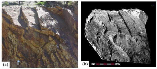
Figure 1.
Road cut slope in case study A. (a) Image from the Rockbench repository and (b) post-processed point clouds dataset.
2.2. Case Study B
The dataset utilized in case study B (Figure 2) was obtained from research conducted in Padua, Italy. This information was supplied by researcher Siefko Slob [34], with field data acquisition performed by Alessia Viero and Antonio Galgaro, both affiliated with the Geosciences Department at the University of Padova. The point cloud comprises 140,677 points, with an average point density of 448 points/m3.
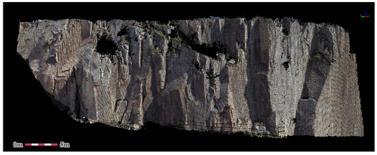
Figure 2.
Point clouds data of case study B.
2.3. Case Study C
Case study C (Figure 3) presents a dataset collected at the entrance of an adit—a horizontal access tunnel—within a rock slope on Niushou Mountain, Qingtongxia City, Ningxia Hui Autonomous Region, China. The rock mass in this area displays considerable structural heterogeneity, marked by localized faulting and folding, distinct bedding planes, and minor fracture zones. Such geological intricacy renders the site particularly suitable for evaluating and validating algorithmic performance. Data acquisition was performed using a Z + F IMAGER 5010C 3D laser scanner (Zoller & Fröhlich GmbH, Wangen im Allgäu, Germany), which operates at a scanning rate of 1,016,000 pixels per second with a linear error under 1 mm. After pre-processing steps, including cropping and resampling, the final dataset used for analysis comprised 1,554,409 points.
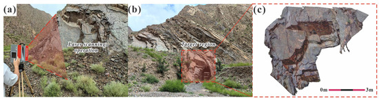
Figure 3.
Data acquisition for case C. (a) general scope of laser scanning, (b) target region of the slope, and (c) point clouds data acquisition results.
3. Methodology
3.1. Discontinuity Segmentation and Boundary Extraction
To detect discontinuity intersection lines, individual discontinuity extraction must first be performed. Notably, individual discontinuity extraction typically follows two strategies: 1. Sets-first segmentation: Clustering dominant discontinuity sets first, followed by isolating individual discontinuity within each set [35,36,37,38]; 2. Plane-first segmentation: Directly extracting individual discontinuity before sets clustering [39,40,41,42]. The sets-first approach risks misclassification in cases where multiple sets intersect within a single discontinuity. This occurs because discontinuities often exhibit intricate 3D geometries—minor protrusions or curvature variations may cause erroneous assignment to incorrect clusters during global clustering. Additionally, the cumulative errors from this two-step process can degrade final accuracy. Moreover, for intersection line detection, contour-point fitting outperforms whole-discontinuity analysis by better preserving geometric features while improving computational efficiency. Therefore, our ARCG method simultaneously accomplishes discontinuity segmentation and contour extraction to facilitate subsequent intersection line detection.
3.1.1. Three-Dimensional Feature Parameter Calculation
The core elements of ARCG are seed point selection and growth criteria determination. These steps must be quantified using 3D spatial features. Therefore, this study employs normal vectors and curvature as the key characterization parameters.
- (1)
- Normal Vector Calculation
While PCA (Principal Component Analysis) efficiently computes normal vectors for large-scale point clouds by evaluating data trends through eigenvalues, its neighborhood matrix construction tends to smooth normal vectors at sharp rock discontinuities, causing distortion. To address this, we implement Robust Randomized Hough Transform [43], which significantly improves normal estimation robustness at discontinuities.
As depicted in Figure 4, Robust Randomized Hough Transform also initiates computation from neighborhood points (the arrows in the figure indicate the normal vectors of the corresponding planes). As illustrated, its distinctive feature involves the following: within a given central point’s neighborhood, randomly selecting two non-collinear points (, ) to form a triplet with the center point. This triplet constitutes a computational unit, where the cross product of internal edge vectors and yields the unit’s normal vector (where , ). To record the distribution of normal vectors, we adopt a spherical accumulator for statistical convenience, following the comparative analysis of different accumulators [44]. As more triplets are constructed, the resulting normal vectors increasingly approximate a normal distribution. However, the number of possible triplets in a point set scales cubically with the number of points (≈n3). Thus, when the normal vector distribution stabilizes within a specific range, we terminate triplet generation and proceed to the next target point, assuming convergence to the correct normal vector. Here are some important definitions: Let be the number of accumulator grid cells, be the number of triplets. For the current grid cell and triplet , they satisfy an independent statistical distribution , where = 1 when vote is assigned to triplet , and = 0 otherwise. Furthermore, Let be the empirical mean value of votes for grid, be the true value, be the distance between two, be the confidence score, be the minimum triplet threshold (stopping criterion). The relationship between and is given by the following empirical formula:
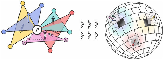
Figure 4.
Schematic diagram of Robust Randomized Hough Transform.
By applying Hoeffding’s inequality to Equation (1), we derive the probabilistic relationship between the and the aforementioned parameters as follows:
The construction process terminates when the triplet count satisfies , whereupon the grid cell with the highest accumulator votes is selected, and its mean value is adopted as the target point’s final normal vector. To mitigate grid discretization effects during voting—where the distribution peak may coincide with grid boundaries—we implement an accumulator rotation strategy. Experimental results demonstrate that five rotations with 5° increments effectively neutralize this artifact.
- (2)
- Curvature Calculation
While conventional curvature computation relies on surface polynomial fitting, this study adopts normal vector variation within local neighborhoods to quantify curvature—achieving more precise 3D curvature characterization while maintaining explicit relationships with normal vectors. As formalized in Equations (3) and (4) as follows:
where denotes the normal vector of the target point, represents the normal vector of any neighboring point, indicates their included angle, and specifies the neighborhood point count.
3.1.2. Adaptive Region Contour Growing
Region growing and plane fitting methods are widely used for individual discontinuity segmentation. Originally developed for image segmentation, region growing algorithms identify areas of interest based on user-defined criteria. This approach proves particularly suitable for rock mass discontinuities due to their distinct planar characteristics. Compared to static iterative formulas in surface fitting, user-defined growth criteria better preserve geometric details of discontinuities. However, traditional region growing requires manual selection of multiple thresholds. This often leads to discontinuities being prone to over-segmentation or under-segmentation, and requires continuous parameter tuning through trial and error to achieve satisfactory results. Furthermore, after completing the segmentation of a single plane, the extraction of the discontinuities contour—also a crucial step for characterizing its 3D morphology—increases the time cost when these steps are executed sequentially. To address this limitation, we propose an adaptive thresholding method, Adaptive Region Contour Growing, that automatically identifies discontinuity by specifying only the value ranges for normal vectors and curvature thresholds. This study introduces another key enhancement: conventional point-cloud contour extraction methods exhibit significant limitations when handling concave discontinuities with complex geometries. Current approaches (e.g., alpha shape, convex hull, Delaunay triangulation, and meridian-parallel scanning) fail to simultaneously address manual parameter tuning requirements, and mixed convex-concave boundary preservation. Moreover, these methods typically require complete discontinuity segmentation before contour extraction. To overcome the rigidity of fixed thresholds and cumbersome post-processing, we propose a mobile spatial contour scanning method integrated with adaptive region growing. This simultaneously performs complex discontinuity identification, and contour point cloud extraction. By eliminating the need for full-discontinuity participation in intersection calculations, computational efficiency is significantly improved. The methodology ARCG comprises the following:
Step 1: The algorithm initiates by sorting all computed curvature values in ascending order and selecting the point with minimum curvature as the initial seed point
Step 2: For each neighboring point , two growth criteria are sequentially evaluated: the angle between ’s normal vector and ’s normal vector—if exceeds a predefined threshold , is classified as a pending point , otherwise it is added to the seed queue;
Step 3: Evaluate the other growth criteria: curvature difference , if it is below threshold , becomes an accessory seed point , otherwise it is marked as a boundary point .
Step 4: Upon encountering , the algorithm records it as the current contour point and calculates its projection vector with the initial seed point onto the plane defined by ’s normal.
Step 5: Subsequent boundary point undergo vector comparison: if and the inter-vector angle is below threshold, replaces ; otherwise, it is appended as a new contour point.
Figure 5 illustrates the parallel processing pipeline for region growing and boundary point extraction.
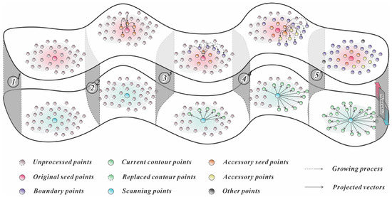
Figure 5.
Adaptive Region Contour Growing algorithm.
To handle complex concave polygons, after completing boundary point scanning, we project the regional points onto a 2D plane centered on the initial seed point and randomly partition subspaces. When encountering discontinuous boundary points within a subspace characterized by small-angle projection vectors with significant modulus differences, the system identifies boundary point defects. Since the discontinuity has already undergone preliminary segmentation, we then apply K-means++ clustering to divide the point cloud into two clusters. The cluster centroid farther from the initial seed point becomes the new scanning location. The newly acquired boundary points merge with original points after deduplication to form the final boundary point set.
Notably, to enable dynamic adjustment of the normal vector threshold, we define an adaptive threshold (Equation (5)):
where and denotes the prescribed maximum and minimum threshold bounds, represents the current regional point count, and is a scaling factor controlling the growth rate, its value is related to the point cloud density and the size of the currently grown region. Here, the is defined as the square of the ratio between the maximum distance between any two points in the current region and the average point spacing. When the region begins to grow, a strict angular tolerance () is maintained, close to . When the region becomes sufficiently large, the tolerance is appropriately relaxed according to Equation (5).
The adaptive curvature threshold follows Equations (6)–(10):
where is the curvature value set within the current region, represents the prescribed lower curvature threshold bound; represents the regional consistency factor, where represents the standard deviation of curvature within the current region and represents the global standard deviation of curvature; represents the neighborhood connectivity factor, where represents the average neighborhood connectivity count; represents the curvature distribution skewness factor, where is the mean curvature within the current region and is the median curvature within the region.
A critical observation is that during region growing, normal vectors determine point inclusion while curvature governs seed point selection, giving normal vectors higher decision priority. The adaptive normal threshold employs a progressive growth function: it maintains strict angular tolerance during initial growth (when point counts are low) to ensure planar accuracy, then gradually relaxes constraints as the region expands to accommodate minor discontinuity undulations. Similarly, the adaptive curvature threshold is designed to remain robust against local protrusions and data noise.
Since our method requires a threshold range, the normal vectors threshold range was set to 5–20°, consistent with empirical values from prior studies [21,22]. For curvature thresholding, we first analyze the curvature distribution and apply K-means++ clustering (k = 2) to separate non-planar points (higher curvature) from planar points (lower curvature). The first cluster (lower curvature, 0.01–0.16) was classified as planar points, while the second (higher curvature) was classified as non-planar points. Thus, the curvature distribution after clustering (Figure 6) justifies this threshold range: 0.01–0.16 (the dataset comprises 91.82% planar points and 8.18% non-planar points).
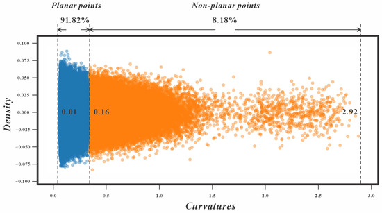
Figure 6.
Curvature cluster distribution.
For comparative evaluation, we selected the conventional region-growing algorithm for discontinuity segmentation (noting that ARCG performs both discontinuity and boundary extraction simultaneously, though it can execute discontinuity segmentation alone if boundary extraction is disabled). We also employed the widely used alpha-shape algorithm for boundary point extraction. Both methods were systematically compared with our proposed approach. As illustrated in Figure 7, the conventional region-growing algorithm requires iterative parameter tuning, frequently leading to under-segmentation or over-segmentation of discontinuities. This necessitates additional post-processing steps such as re-segmentation or merging operations. Similarly, the alpha shape algorithm demands repeated parameter adjustments to identify optimal values. In contrast, our method dynamically adapts thresholds to local conditions while simultaneously extracting boundary points, achieving both precision and computational efficiency in automated extraction.
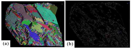
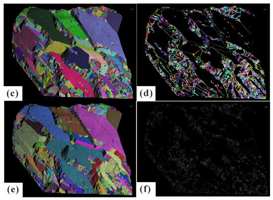
Figure 7.
Comparison of discontinuities segmentation and contour extraction between proposed method and traditional region growing with alpha-shape. (a,b) results of over-segmentation and alpha shape; (c,d) results of proposed method; (e,f) results of under-segmentation and alpha shape.
3.2. Determination of Discontinuity Intersection Relationships
3.2.1. Selection of Relatively Optimal Model
After extracting boundary point clouds of discontinuities, the subsequent step involves determining intersection relationships between discontinuities and identifying their intersections through adjacent boundary point clouds. However, the massive volume and lack of topological information in point clouds make automatic coordinate-based searches impractical, necessitating spatially representative models to characterize the 3D distribution of each discontinuity. The classical Baecher disk model [45], derived from Robertson’s analysis of approximately 9000 trace lengths in the DeBeer open-pit mine slope (South Africa), offers a computationally efficient solution. This model requires only three parameters (center coordinates, radius, and normal vector) to generate simulations. Its effectiveness in determining intersection relationships has led to widespread application in DFN (Discrete Fracture Network) modeling and rock block analysis [46,47,48]. Alternative discontinuity modeling approaches exist, including the 1955 orthogonal model [49] that represents discontinuities as two or three sets of mutually perpendicular, infinitely extending planes. However, this representation proves inadequate for analyzing intersection relationships. Some researchers have adopted polygon models [50] to better approximate real-world discontinuities, using intersection relationships to identify rock blocks. The ellipse models [51], proposed contemporaneously with the disk model, failed to gain widespread acceptance due to its inherent limitations compared to circular representations. Later studies [52,53] demonstrated that elliptical disk models can effectively simulate discontinuities when considering trace length distributions, proving particularly suitable for certain discontinuity exposure patterns. Collectively, these studies confirm that discontinuities can be represented through various geometric models, though no consensus exists regarding an optimal solution—model selection remains context-dependent. Therefore, when analyzing spatial intersection relationships of discontinuities, this study evaluates multiple geometric models to identify the optimal representation, quantitatively assessing simulation accuracy through the Area Ratios metric. It should be noted that all model computations are fundamentally based on the minimum convex hull polygon derived from discontinuity boundary point clouds. Accordingly, we define Area Ratios as follows:
where represents the area of the fitted geometric model, denotes the actual area of the minimum convex hull enclosing the discontinuity boundary points.
This section evaluates six geometric models (circle, ellipse, rectangle, parallelogram, parallel hexagon, and arbitrary trapezoid), all calculated using minimum bounding geometry. The model selection criteria consider geological evidence showing discontinuities typically exhibit polygonal, irregular quadrilateral, or banded morphologies [46]; tectonic stress-induced discontinuities often display directional extension (e.g., conjugate joint systems), where parallelogram/hexagonal models better capture anisotropic characteristics; mathematical considerations: point cloud data inherently represents discontinuity boundaries as discrete points forming complex polygons—while more complex models provide better theoretical fits, they incur significant computational costs, making simple parallel polygons optimal for balancing directional accuracy and efficiency. From the 1260 individual discontinuities obtained in Section 3.1.2, we calculated AR for each model fit using extracted boundary points (distribution shown in Figure 8). The pseudocode for models fitting is provided in the Supplementary Materials (Algorithms S1–S8).
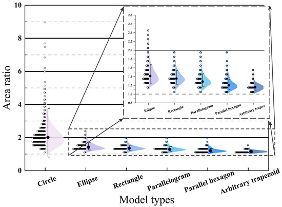
Figure 8.
Violin plots of area ratios of different discontinuities models.
Beyond the AR, fitting efficiency serves as another key metric for model evaluation. Table 1 summarizes the median, quartiles, and computation time of AR distributions for each model.

Table 1.
Various indicators of different discontinuities models.
The disk model exhibits distinct AR characteristics: its median AR is nearly double that of other models, indicating systematic overestimation of 3D discontinuity area and directional extension. This leads to artificially isotropic fitting results. Its broader distribution width (higher IQR (interquartile range)) reveals greater AR variability, demonstrating heightened sensitivity to complex discontinuity geometries. The disk model’s platykurtic distribution reflects unstable fitting performance, whereas other models exhibit leptokurtic distributions with tightly clustered AR values. A pronounced right-skewed tail suggests that the disk model generates excessive area estimates when fitting elongated discontinuities. Polygonal models show stable AR trends: ellipse > rectangle > parallelogram > parallel hexagon > arbitrary trapezoid. Geometrically, increased edge complexity (e.g., arbitrary trapezoids requiring only one parallel edge pair) correlates with lower AR and improved discontinuity characterization.
Figure 9 illustrates a representative zone from case study A, and Figure 10 illustrates the fitting performance of all six models of the zone. Key discrepancies include the following: Figure 10a, disk model falsely intersects discontinuities 1 and 25; Figure 10c–f, overfitting in polygonal models misclassifies discontinuities 37 and 29 as non-intersecting; and Figure 10e, hexagons marginally reduce area coverage compared to parallelograms without significant spatial extension changes. It is therefore evident that the spatial intersection results vary significantly across different models. Therefore, in addition to the Accuracy Rate (AR), this paper also proposes the Intersection Line Endpoint Error Rate (ILEER). For a given potential intersection line, different models compute different 3D coordinates for its start and end points. The ILEER is calculated as follows:
where is the length of the actual trace line, and is the length of the intersection line from the fitted model.
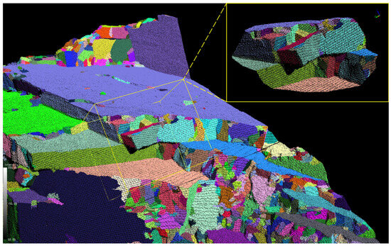
Figure 9.
Representative zone from case study A.
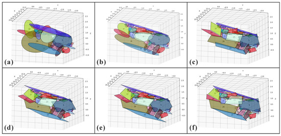
Figure 10.
Fitting effect of representative zone of different discontinuities models. (a) disk models; (b) ellipse models; (c) rectangle models; (d) parallelogram models; (e) parallel hexagon models; (f) arbitrary trapezoid models.
Using the sample region from Figure 9 as the test case, the average IPERL for each model and the ILEER for selected intersection pairs are shown in the table. The ranking (from highest to lowest ILEER) is as follows: parallelogram > ellipse > parallel hexagon > rectangle > arbitrary trapezoid > circle. Some ILEER values are 0 because the model fits the planar surface very well, resulting in no intersection being detected between two adjacent discontinuities. This is also why the ILEER for the rectangle and trapezoid models is relatively low. For the disk model, its low ILEER is due to an excessively large AR, which leads to an overly long computed intersection line.
Therefore, by synthesizing the data from Table 1 and Table 2, we can observe that the parallelogram, parallel hexagon, and ellipse models all demonstrate satisfactory fitting performance, making them relatively suitable for intersection line calculation. To achieve both efficient geometric fitting and preserve spatial extensibility of discontinuities, this study adopts the parallelogram model for subsequent discontinuity intersection analysis.
Table 2.
ILEER of intersecting pairs selected and average ILEER of different models.
3.2.2. Discontinuity Intersection Analysis
Given the large number and random spatial distribution of discontinuities in 3D space, exhaustive pairwise intersection calculations would be computationally prohibitive. Thus, a preliminary spatial distance filter is essential to reduce the candidate set. The filtering criterion evaluates whether the centroid distance between two discontinuities is less than the sum of their : radius for disks, semi-major axis for ellipses, and half the longest diagonal for polygons (rectangles, parallelograms, parallel hexagons, and arbitrary trapezoids). This spatial pre-screening significantly reduces the number of potential intersection pairs for each discontinuity, after which true/false intersection verification is performed. As illustrated in Figure 11 (demonstrated here for ellipses), the verification method involves the following: (1) computing the intersection line of the two discontinuities; (2) discarding pairs where either discontinuity intersects this line at fewer than two points (false intersections); and (3) for pairs with two intersection points per discontinuity, connecting these points into segments—spatial overlap between segments confirms a true intersection. Post-screening intersection configurations fall into five primary spatial relationships (excluding special cases like tangency or single-point contact).
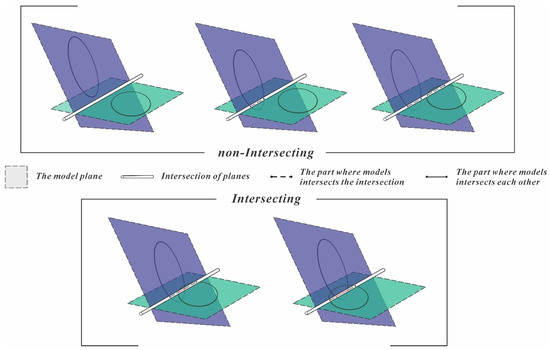
Figure 11.
Five types of discontinuities intersection pairs.
3.3. Trace Extraction and Vectorization
3.3.1. Trace Fitting
After identifying intersecting discontinuity pairs in 3D space, their intersection lines must be extracted. However, since discontinuities are already segmented, trace positions cannot be accurately determined from a single discontinuity alone. Moreover, if a trace is constructed by directly connecting point clouds, the point association problem becomes non-trivial. To address this, our method connects traces using the spatial geometric centers of contour points from both discontinuities. The procedure consists of four main steps:
Step 1: First, the contour point set of one discontinuity is used as the search set, and a KD (K-Dimension) tree is constructed to establish neighborhood relationships. Points from the other contour set are searched within a specified radius (adjusted adaptively if the searched set has significantly lower point density). The roles of two point sets are then reversed. This yields two spatially proximate linear point clusters. Due to the inherent sparsity and noise in point clouds, DBSCAN (Density Based Spatial Clustering of Applications with Noise) is applied to each set for denoising (with empirically determined parameters: eps = three times the average point cloud spacing, minpts = 4);
Step 2: The centroids of the denoised point sets (Equation (13)) are computed, and PCA corresponding to the largest eigenvalue defines the directional vector of each point set. By anchoring this vector at the centroid, a 3D line is derived to represent the linear point cluster.
Step 3: Construct a fitting line using the mean centroid and directional vector of the two point sets. Project all points onto this line, then define a segment bounded by the most distant projected points. The segment is then divided into equidistant sub-segments, with the number of subdivisions determined by both total segment length and local point density
(Equations (14) and (15)):
where the is adaptively optimized based on point density variations, where represents the global average point density and ⌊ ⌋ represents round down. A minimum sub-segment length of 0.04 m (user-defined) ensures preservation of trace geometry, while the formulation guarantees at least 4 sub-segments;
Step 4: After determining the appropriate number of segments based on length and point density, the centroid point of the point set within each segment of length is calculated. These centroid points are then sequentially connected to form the trace between the two discontinuities, which appears as a polyline.
The segmentation process is illustrated in Figure 12.
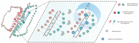
Figure 12.
Discontinuities intersection pairs fitting trace segments.
3.3.2. Trace Segments Connection
Since trace segments are derived from pairwise discontinuity intersections, they typically exhibit fragmented distributions. To obtain a continuous trace, segment connection is required. Existing methods predominantly use point clouds as basic units, employing least-cost-path [26], MS-LBP [27], or weighted feature-based linear growth algorithms [54]. For trace segments specifically, some studies connect discontinuous segments using multi-criteria parameters (e.g., angular/distance thresholds) to prioritize longer linear traces [24]. However, these approaches risk erroneous connections due to trace sparsity. Our method instead treats all trace segments from the same discontinuity as connection candidates, using a bidirectional weighted graph-based growth algorithm (Figure 13) with the following steps.
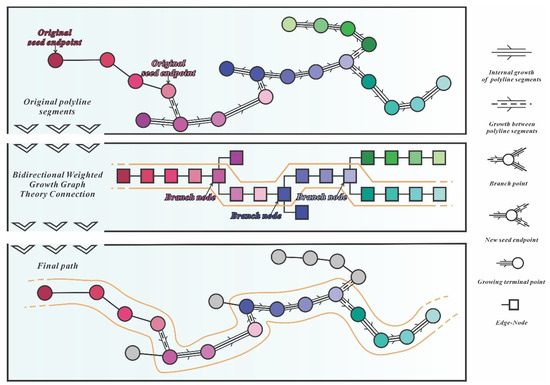
Figure 13.
Bidirectional weighted graph-based growth algorithm.
Step 1: Create a temporary global index of all trace segments for the target discontinuity, then construct a KD-tree using each segment’s point cloud;
Step 2: Designate the longest segment as the original seed segment, with its two endpoints as original seed points. For each seed, search for neighboring points within a specified radius via KD-tree query. If multiple points belong to the same segment, select the nearest one. Terminate the search if no points are found (indicating an endpoint) and log processed segments to avoid redundancy;
Step 3: Assess the positional relationship of matched points: (a) if a point is a segment endpoint, treat it as a new seed (return to Step 2); (b) if it is a mid-segment point, extend connections to both endpoints and repeat Step 2 for each;
Step 4: During growth, construct an undirected graph where nodes represent point coordinates and edges denote connections. For endpoint links, record edges directly; for mid-segment links, split the node path;
Step 5: After bidirectional searches from the initial seed, merge the two subgraphs by connecting nodes via the seed segment;
Step 6: Assign weights to paths based on length, node count, and angular deviation (Equation (16)). The optimal trace is identified as the highest-scoring path via Dijkstra’s algorithm on the weighted graph.
where represents the length of the candidate path, represents the summed length of all nodes, is the node count in the candidate path, is the total node count, denotes the maximum angular deviation along the path. represent the length weighting coefficient, node count weighting coefficient, and angle penalty weighting coefficient, respectively.
In contrast, traditional path-search methods, such as the MST (Minimum Spanning Tree), forcibly connect all points into a single structure using the shortest edges, aiming to minimize the global connection cost. However, when a region contains a long primary trace and several shorter branch traces, the MST fails to prioritize the integrity of the primary trace. In contrast, the method proposed in this paper is inclined to explore longer paths. Starting from a seed point located on a dominant discontinuity, the algorithm grows by evaluating multiple weighting metrics, thereby extracting the entire primary trace completely, and effectively preserving the dominant trace that reflects the true scale of the discontinuities.
4. Results and Discussion
4.1. Extraction Results and Comparison
The proposed ARCG, model fitting and bidirectional weighted graph-based growth algorithm, etc., was implemented in Python Jupyter Notebook 3.9.12. The implementation relied on Qt, the Open3D, the NumPy, SciPy. Furthermore, the qualitative comparison and manual inspection of 3D trace reconstructions were performed using CloudCompare (v2.12.4). All experiments were conducted on a standard laptop computer (13th Gen Intel Core i5-13500HX processor, 16.0 GB DDR memory, 64-bit Windows system).
4.1.1. Case Study A: Extraction Results and Comparative Analysis
Case study A, a widely cited open-source dataset in rock discontinuity research, contains both well-developed and fragmented discontinuities with trace. Its balanced representation makes it an ideal benchmark, enabling direct comparison of our method with existing approaches. Figure 14 illustrates the comparative results as follows: (a) presents trace extraction using the proposed method; (b) shows Li’s [25] approach, which employs NTV to detect trace feature points from 3D point clouds. These points are grouped by geometric similarity, with PCA determining principal orientations. A region-growing algorithm connects points into segments, followed by merging fragmented traces and pruning outliers deviating beyond angular thresholds; (c) demonstrates Guo’s method [54], where potential feature points are identified via 1D truncated Fourier series with curvature thresholds. Points undergo curvature-weighted Laplacian smoothing before being connected using a feature-parameter-weighted line-growing algorithm; (d) displays Zhang’s [24] technique, which shares initial steps with Li et al. but innovates by enforcing geometric rules for trace continuity, segmenting nonlinear connections into linear sub-traces, and merging segments using axial and radial distance and curvature criteria. However, the results of the NTV method depend on the resolution of the triangular mesh. If the resolution is too low, computational efficiency is high, but it blurs the details of the discontinuities. If the mesh resolution is too high, even with improved connection methods, it becomes difficult to handle complex scenarios for trace extraction. Consequently, it can only extract relatively prominent traces (as shown in Figure 14b,d). On the other hand, the 1D truncated Fourier series method can identify two types of traces based on different curvature directions, but it faces significant difficulty in establishing the connection relationships between them. The two types of traces remain discrete, and lack a clear affiliation with the discontinuities.
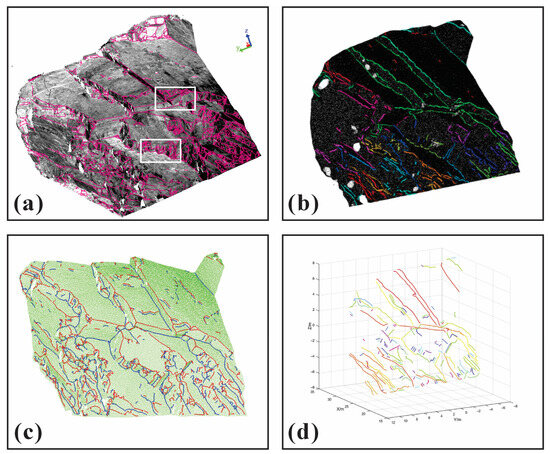
Figure 14.
Comparison between the proposed method and existing methods of case A. (a) discontinuity trace extracted by proposed method; (b) discontinuity trace extracted by Li’s method of NTV; (c) discontinuity trace extracted by Guo’s method of 1D truncated Fourier series; (d) discontinuity trace extracted by Zhang’s method of modified NTV.
All four methods successfully identify primary discontinuity traces, as demonstrated in Figure 14. The proposed method demonstrates superior performance by extracting traces through confirmed discontinuity intersections, which establishes clear trace-to-parent relationships, and maintaining better trace continuity through specified discontinuity connections. In contrast, comparative methods produce fragmented traces with noticeable discontinuities (Figure 14b–d). While existing methods [24,25,54] efficiently detect feature points via triangular mesh or point cloud curvature analysis, they struggle in complex zones with fragmented discontinuities. Their principal limitation lies in the initial feature detection phase, where planar regions are often misclassified as trace points, leading to omission of short traces. Our approach excels in challenging regions (Figure 14a, white rectangle) through precise individual discontinuity segmentation of small discontinuities, and enhanced detection of subtle traces via intersection lines. This dual mechanism captures fine-scale features missed by curvature-based methods.
To assess the enhancement in trace connectivity resulting from our approach, specific metrics are necessary to characterize its practical effectiveness beyond visual analysis. Conventional validation measures like F1-score and recall are generally intended for binary classification tasks. In contrast, the extraction of discontinuous traces prioritizes precision in geometric morphology, often neglecting spatial configurations. Consequently, this study introduces topological corners at the intersections of traces as a means to quantitatively evaluate the connectivity of the outcomes. At the junction where multiple discontinuities intersect, a topological corner forms, serving as a connection point for several traces. A corner is deemed valid only when all trace segments linked to it have been accurately extracted. To assess the overall connectivity of these identified corners, we employ the topological connectivity rate as our evaluation metric as follows:
denotes the topological connectivity rate, denotes the number of corner points meeting topological conditions, denotes the total number of corner points selected.
In case A, Figure 15 and Table 3 illustrates 42 significant topological corners alongside detailed regional views. Our method achieves a topological connectivity rate of 90.48%, substantially outperforming the alternative approaches, which yield rates of 14.29%, 40.48%, and 9.52%, respectively.
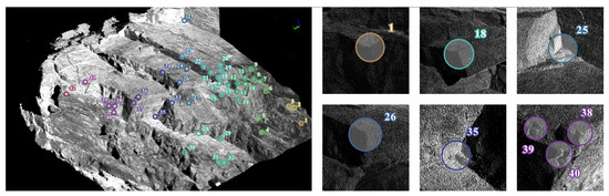
Figure 15.
Selection of topological corner points and partial detail regions in case A.
Table 3.
Topological connectivity rate of proposed method and existing methods in case A.
4.1.2. Case Study B: Extraction Results and Comparative Analysis
Case study B serves as another benchmark for discontinuity and trace extraction methods. Guo et al. [27] proposed an approach for this dataset involving converting RGB point clouds to grayscale to detect color-gradient boundaries as potential trace points, applying MS-LBP to mitigate illumination shadows by analyzing eight-quadrant voxel intensity contrasts, and connecting traces via a bidirectional local vector buffering algorithm with shadow processing. We further benchmark against Thiele’s Compass plugin [26] for CloudCompare (an open-source platform for point cloud processing including denoising, geometric fitting, and feature extraction). Having compared our method with three alternative approaches in the preceding section, we focus here on benchmarking against Guo’s method and Thiele’s method (Figure 16). Subfigures show the following: (a) ARCG individual discontinuity segmentation, (b) result of proposed method, (c) Guo’s MS-LBP results, and (d) results of Thiele’s method on CloudCompare. Guo’s method can eliminate the influence of shadows and extract fault traces on smooth surfaces by utilizing the color information of the point cloud. However, it performs well only under specific conditions where shadows are present. Thiele’s method requires the selection of trace starting points, and the algorithm automatically connects the trace paths. However, the selection of starting point locations is influenced by subjective experience, leading to low extraction efficiency. Moreover, the topological connectivity rates of both methods are lower than that of our proposed method.
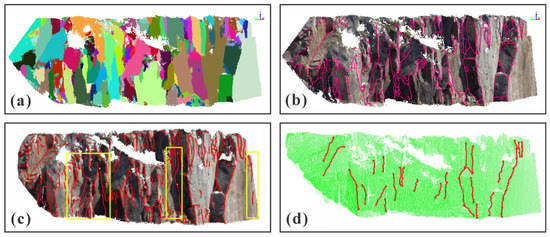
Figure 16.
Comparison among the proposed methods and existing methods of Case B. (a) discontinuity segmentation result by ARCG; (b) discontinuity trace extracted by proposed method; (c) discontinuity trace extracted by Guo’s method of MS-LBP; (d) discontinuity trace extracted by CloudCompare.
Quantitative comparison with Guo’s published CloudCompare results (Table 4 demonstrates our method’s 44.8% efficiency gain). Area density is calculated per Equation (18):
where is the total length of 2D projected trace, is the area of 2D projection plane.
Table 4.
Comparison among the proposed method, existing method and CloudCompare.
Comparative analysis reveals our method detects all reference trace with superior connectivity. As shown in Figure 17 and Table 5, the 22 topological corners selection and the topological connectivity rate for case B. The topological connectivity rate of our method reaches 90.91%, while those of the other methods are 36.36% and 9.09%, respectively.
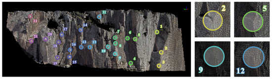
Figure 17.
Selection of topological corner points and partial detail regions in Case B.
Table 5.
Topological connectivity rate of proposed method and existing methods in case B.
4.1.3. Results and Computational Verification of Case C
To assess the precision of the introduced algorithm, its output trace was evaluated against manually drawn results using several quantitative measures. It is important to note that the proposed approach maintains trace connectivity with well-established topological associations before this phase, meaning that separating the structure at branching locations is adequate to obtain distinct trace segments. By synthesizing graphical and tabular outcomes, it is clear that the method delivers correct identification in both detection accuracy and coverage. As indicated in Figure 18c and Table 6, the selection of 24 topological corners and the topological connectivity rate for case C are presented. The topological connectivity rate attained by our technique is 91.97%. According to Table 7, the area density for case C using the proposed method is 2.11 m. Additionally, when compared with manual delineation outcomes, the longest trace exhibits a length error rate of 9.01% (the shortest trace is insufficiently long for a valid assessment). Moreover, because of the variable development of discontinuities and the intricate arrangement of traces in this particular case, the dataset shows a broad spectrum of individual trace length error rates, spanning from 9.45% down to 3.64%.
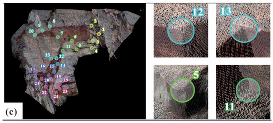
Figure 18.
Trace detection and validation of case C. (a) discontinuities segmentation results, (b) detection results and (c) selection of topological corner points and partial detail regions in case C.
Table 6.
Topological connectivity rate of proposed method and existing methods in case C.
Table 7.
Computational verification of proposed method and manual delineations.
4.2. Discussion
The three aforementioned mainstream methods can be fundamentally categorized into two paradigms. The first one is a data-feature-driven approach that extracts traces from curvature, normal vectors, or RGB and grayscale values in pixels, point clouds, or triangular meshes, and the other one is a definition-driven method like ours that identifies traces as intersection sets of discontinuities.
4.2.1. Practical Limitations of the Method
Compared to feature-based methods that are noise-sensitive, our approach offers distinct advantages: explicit trace-to-discontinuity correspondence, and the capability to group traces by orientation and identify dominant discontinuity sets in rock masses. However, while our intersection-based method captures most traces accurately. However, the current approach has the following limitations:
1. Weathering-induced small discontinuities fully enclosed within larger ones may be misclassified as true intersections. As shown in Figure 19a, the large discontinuity contains numerous minor discontinuities. Figure 19b demonstrates that if based on 3D characteristics, the trace corresponding to these protrusions can be correctly extracted. However, using the ARCG single-plane segmentation method proposed in this paper, these protrusions are misidentified as small, independent discontinuities (Figure 19c). The distribution of these small planes depends on the algorithm’s recognition efficacy, and they exhibit an inclusion relationship within the larger discontinuity. Consequently, the resulting trace, as shown in Figure 19d, appears fragmented and discontinuous, only present at the locations of these small discontinuities. In reality, most of these small features are likely caused by weathering, and compared to the scale of the large discontinuity they belong to, should not be identified as discrete discontinuities. Moreover, they should not be included in the calculation of the dominant set, as they do not affect the overall stability.
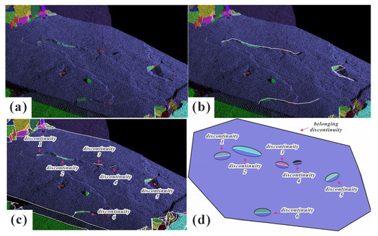
Figure 19.
When the discontinuities are in an inclusion condition. (a) overall perspective, (b) correct trace identified based on 3D characteristics, (c) results from the proposed method and (d) simulated inclusion relationships of discontinuities.
Therefore, a subsequent improvement to the method is proposed. When a discontinuity is identified as being excessively large and completely encompassing other smaller discontinuities, the latter should be removed following a visual inspection to confirm their nature. Trace detection utilizing 3D characteristics should then be re-performed on the refined dataset.
2. Due to the varying degrees of development of discontinuities, even though the ARCG method in this study can effectively identify the boundaries of individual discontinuities, relying solely on intersection relationships to fit the locations of traces is still insufficient to account for all complex scenarios. As shown in Figure 20a,b, discontinuity 2, although exhibiting a complex morphology, has a relatively concentrated overall curvature distribution, with a mean curvature value significantly lower than the set threshold. Therefore, ARCG correctly identifies it as a single plane. This observation is also commonly encountered in existing discontinuity identification workflows. As shown in Figure 20c, if we simulate the intersection relationships, it can be seen that there is only one intersection line between the two discontinuities; however, Figure 20d (from manual interpretation) shows an additional intersection line that was not detected.
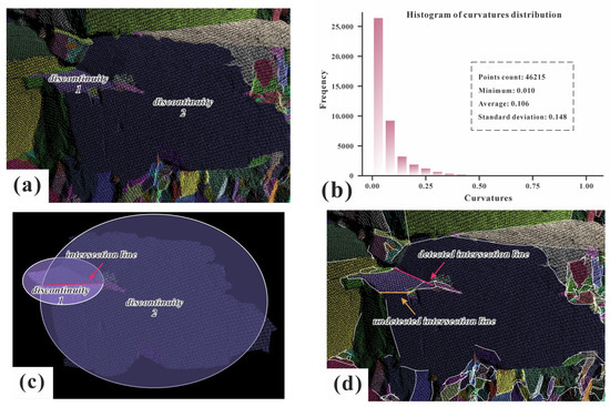
Figure 20.
Complex discontinuities trace identification results. (a) discontinuities adjacency scenario, (b) curvature distribution histogram of discontinuity 2, (c) discontinuities model fitting and (d) trace extraction discrepancies.
For discontinuities with complex boundary morphologies, relying solely on intersection relationships is insufficient to identify all traces, and requires supplementary information from 3D characteristics. Furthermore, some traces cannot be derived from intersection relationships and do not exhibit distinct 3D characteristics. For example, the trace within the rightmost yellow rectangle in Figure 16 was not identified by the present method. This trace only exhibits a slightly darker color compared to the surrounding discontinuities. But any single method has its limitations. The geometric analysis serves as the primary, most reliable tool, and is seamlessly supplemented by other data sources (like RGB) when geometric features are ambiguous.
In summary, the performance of this method is compromised when dealing with the following: (1) inclusion relationships within large discontinuities, (2) discontinuities with complex boundaries, and (3) cases requiring RGB-assisted identification, where its identification effectiveness is diminished.
4.2.2. Extraction Effect of Proposed Method
- 1.
- Efficiency for data of different magnitudes
In practical engineering contexts, the collection of point clouds from large-scale excavations or exposed rock slopes frequently results in datasets containing millions to hundreds of millions of individual points.
While the proposed method demonstrated high computational efficiency in previous comparisons, its processing time is highly dependent on point cloud density. To quantitatively evaluate this relationship, we conducted tests using a dataset containing 9,508,395 points. As indicated in Table 8, the dataset was systematically resampled at multiple percentage resolutions based on mean point spacing, and the corresponding runtimes were recorded.
Table 8.
Runtimes under multiple percentage resolutions of point clouds.
As can be observed from the table, when the point cloud size reaches approximately 5.7 million points, the processing time per million points remains relatively stable (around 340 to 370 s). However, beyond 7.6 million points, it begins to increase significantly, reaching 680 s per million points at 9.5 million points. Therefore, the current algorithm demonstrates practical engineering utility for point cloud scales of 1 to 5 million points (completing within tens of minutes). However, as the point cloud approaches tens of millions of points, the processing time nears 2 h. For engineering scenarios where real-time results are not typically required post-data acquisition, a processing time of several hours may be acceptable. However, if used for rapid feedback during construction, further optimization must be considered.
- 2.
- Parameter sensitivity analysis of the bidirectional weighted graph-based growth algorithm
In the proposed method, the connection of traces for intersecting pair identification is governed by three weighting parameters (path length, node count, and angle penalty). Therefore, this section discusses the influence of these parameters and their optimal value ranges, with accuracy measured by the number of correctly matched nodes.
As shown in Figure 21, the ablation study is conducted by modifying a single weighting coefficient at a time, using the intersection lines between discontinuity 1 and other planes in the region selected in Figure 13 for validation. In Figure 21b, each intersection line is depicted in a different color (totaling 64 nodes, with 47 being correct).
Figure 21.
Selectd discontinuity and its trace. (a) selectd discontinuity and (b) the intersection lines derived from the selected discontinuity and the discontinuities intersecting with it.
As can be seen from Table 9, the length weight and node count weight are fine-tuning parameters with a limited impact on the path selection. When the length weight is less than 1, it ensures a relatively high path accuracy; however, within the range of 1 to 5, the selection of incorrect paths occurs, and the accuracy decreases as the weight increases. For the node count weight, the same optimal path is obtained when the weight is less than 5, and the accuracy begins to decline within the range of 5 to 10. In contrast, the angle penalty weight leads to the selection of incorrect paths to varying degrees across the tested range of 0.1 to 10. Furthermore, 100% path accuracy is only achieved after further increasing this weight to approximately 20. This indicates that among the three weighting parameters in our algorithm, the angle penalty weight is the critical factor and plays a pivotal role in connecting discontinuous traces.
Table 9.
Ablation study under different weighting coefficients.
- 3.
- The impact of the number of discontinuities segmentation
The proposed method identifies discontinuity traces based on two core components: segmentation of individual discontinuities and intersection relationship analysis. In case study B, we systematically varied individual discontinuity segmentation accuracy by adjusting normal vectors and curvature thresholds. Table 10 documents how these changes affect area density across different discontinuity counts.
Table 10.
The variation in area density with respect to discontinuity counts.
Results demonstrate that trace extraction accuracy is directly governed by discontinuity segmentation quality. This necessitates adaptive algorithms to optimize segmentation, balancing between under-segmentation and over-segmentation. What is more, data acquisition limitations (e.g., scanning angles, occlusions) often yield unclosed discontinuity boundaries, creating edge gaps that prevent complete trace identification. This point-cloud deficiency remains a critical unsolved challenge for most existing methods.
4.2.3. The Performance of Different Discontinuity Models
The discontinuity models selected in this study represent geometrically simple yet geologically meaningful cases. Classical disk and elliptical models assume fixed dip/strike-derived trace lengths, where both the principal axis orientation (rotation angle) and aspect ratio are treated as constants. However, field observations reveal that natural discontinuities exhibit complex geometries, requiring these parameters to be variable. To address this, our elliptical models construct a covariance matrix from discontinuity point clouds, using eigenvectors and eigenvalues to dynamically define principal axes orientations and ratios. For polygonal models (lacking axial symmetry), we prioritize computational efficiency by adopting minimum bounding geometries without rotational correction, given their inherent complexity from multiple edges and vertices. Overly tight fitting (e.g., arbitrary trapezoids) may reduce spatial extensibility, potentially causing false negatives in intersection detection. We propose future refinements using the longest diagonal as a pseudo-major axis with minor angular adjustments to balance accuracy and efficiency.
5. Conclusions
Compared to existing methods that extract traces by computing 3D features from point clouds or triangular meshes, our intersection-based search approach demonstrates superior precision and efficiency. Moreover, given the massive volume and lack of topological structure in point clouds, the proposed method integrates discontinuity segmentation with spatial characteristics, ensuring accurate trace alignment with the 3D model without full reliance on point cloud processing. Key conclusions are summarized as follows:
- (1)
- We propose the ARCG algorithm, which simultaneously performs discontinuity segmentation and contour extraction. By dynamically adjusting thresholds and growth parameters within a predefined range, the method eliminates manual trial and error. During growth, points are classified as seed or boundary points, while iterative angle-threshold updates enable concurrent contour extraction. Compared to conventional approaches, the proposed method simplifies workflow while significantly improving accuracy.
- (2)
- Among the six fitting models evaluated, the conventional disk model is generally unsuitable for characterizing spatial intersections. Rectangles and arbitrary trapezoids suffer from directional inflexibility and edge complexity, respectively, leading to false non-intersection classifications. Parallel hexagons show negligible improvement over parallelograms. Thus, according to the distribution of the two quantitative metrics, AR and ILEER, parallelograms and ellipses better represent discontinuity spatial distributions.
- (3)
- Our point–density-based segmentation preserves geometric features while enhancing edge adherence. The bidirectional weighted graph-based growth method connects trace segments belonging to the same discontinuity using multi-criteria weights and nodal relationships, optimizing true trace extraction. This approach clarifies trace-to-discontinuity relationships, improves connectivity, and achieves a 48.8% efficiency gain over existing methods.
Supplementary Materials
The following supporting information can be downloaded at: https://www.mdpi.com/article/10.3390/rs17213566/s1, Algorithm S1–S8: The pseudo-code of the models fitting. For the sake of reproducibility and clarity is provided alongside this manuscript.
Author Contributions
J.S.: Conceptualization, methodology, formal analysis, data curation, writing—original draft, writing-review and editing, and visualization. Q.X.: Supervision, resources, and project administration. X.D.: Funding acquisition and investigation. H.L.: Formal analysis and methodology. Q.H.: Formal analysis, writing-review and editing, validation, and visualization. B.D.: Writing-review and editing, and visualization. All authors have read and agreed to the published version of the manuscript.
Funding
The work was funded by the National Key R&D Program Key Special Projects (No. 2022YFC3003200).
Data Availability Statement
During the preparation of this work, the authors used Deepseek-R1 (v.0528) for grammar checking and language optimization services. After using this tool, we reviewed and edited the content as needed and take full responsibility for the content of the published article.
Conflicts of Interest
The authors declare that they have no known competing financial interests or personal relationships that could have appeared to influence the work reported in this paper.
References
- Mehrishal, S.; Leem, J.; Kim, J.; Shao, Y.; Kang, I.-S.; Song, J.-J. Tunnel Rapid AI Classification (TRaiC): An Open-Source Code for 360° Tunnel Face Mapping, Discontinuity Analysis, and RAG-LLM-Powered Geo-Engineering Reporting. Remote Sens. 2025, 17, 2891. [Google Scholar] [CrossRef]
- Crosta, G. Evaluating Rock Mass Geometry from Photographic Images. Rock Mech. Rock Eng. 1997, 30, 35–58. [Google Scholar] [CrossRef]
- ISRM. International Society for Rock Mechanics commission on standardization of laboratory and field tests: Suggested methods for the quantitative description of discontinuities in rock masses. Int. J. Rock Mech. Min. Sci. Geomech. Abstr. 1978, 15, 319–368. [Google Scholar] [CrossRef]
- Daghigh, H.; Tannant, D.D.; Daghigh, V.; Lichti, D.D.; Lindenbergh, R. A Critical Review of Discontinuity Plane Extraction from 3D Point Cloud Data of Rock Mass Surfaces. Comput. Geosci. 2022, 169, 105241. [Google Scholar] [CrossRef]
- Battulwar, R.; Zare-Naghadehi, M.; Emami, E.; Sattarvand, J. A State-of-the-Art Review of Automated Extraction of Rock Mass Discontinuity Characteristics Using Three-Dimensional Surface Models. J. Rock Mech. Geotech. Eng. 2021, 13, 920–936. [Google Scholar] [CrossRef]
- Barton, N. Review of a New Shear-Strength Criterion for Rock Joints. Int. J. Rock Mech. Min. Sci. Geomech. Abstr. 1973, 7, 287–332. [Google Scholar] [CrossRef]
- Franklin, J.A.; Maerz, N.H.; Bennett, C.P. Rock Mass Characterization Using Photoanalysis. Int. J. Min. Geol. Eng. 1988, 6, 97–112. [Google Scholar] [CrossRef]
- Lemy, F.; Hadjigeorgiou, J. Discontinuity Trace Map Construction Using Photographs of Rock Exposures. Int. J. Rock Mech. Min. Sci. 2003, 40, 903–917. [Google Scholar] [CrossRef]
- Kemeny, J.; Post, R. Estimating Three-Dimensional Rock Discontinuity Orientation from Digital Images of Fracture Traces. Comput. Geosci. 2003, 29, 65–77. [Google Scholar] [CrossRef]
- Reid, T.R.; Harrison, J.P. A Semi-Automated Methodology for Discontinuity Trace Detection in Digital Images of Rock Mass Exposures. Int. J. Rock Mech. Min. Sci. 2000, 37, 1073–1089. [Google Scholar] [CrossRef]
- Esmaeili, M.; Beni, T.; Gigli, G.; Tofani, V. Rock Mass Exposure Fracture Detection through 2D Close-Range Images Using Image Processing Techniques: A Review. Earth Sci. Inform. 2025, 18, 494. [Google Scholar] [CrossRef]
- Vasuki, Y.; Holden, E.-J.; Kovesi, P.; Micklethwaite, S. An Interactive Image Segmentation Method for Lithological Boundary Detection: A Rapid Mapping Tool for Geologists. Comput. Geosci. 2017, 100, 27–40. [Google Scholar] [CrossRef]
- Wang, S.; Yin, J.; Pi, Z.; Cao, W.; Cai, X.; Zhou, Z. Automatic Detection and Characterization of Discontinuity Traces and Rock Fragment Size Distribution Using a Digital Image Processing Method. Measurement 2024, 228, 114343. [Google Scholar] [CrossRef]
- Lary, D.J.; Alavi, A.H.; Gandomi, A.H.; Walker, A.L. Machine Learning in Geosciences and Remote Sensing. Geosci. Front. 2016, 7, 3–10. [Google Scholar] [CrossRef]
- Chen, J.; Zhou, M.; Huang, H.; Zhang, D.; Peng, Z. Automated Extraction and Evaluation of Fracture Trace Maps from Rock Tunnel Face Images via Deep Learning. Int. J. Rock Mech. Min. Sci. 2021, 142, 104745. [Google Scholar] [CrossRef]
- Chen, J.; Yang, T.; Zhang, D.; Huang, H.; Tian, Y. Deep Learning Based Classification of Rock Structure of Tunnel Face. Geosci. Front. 2021, 12, 395–404. [Google Scholar] [CrossRef]
- Chen, J.; Huang, H.; Cohn, A.G.; Zhang, D.; Zhou, M. Machine Learning-Based Classification of Rock Discontinuity Trace: SMOTE Oversampling Integrated with GBT Ensemble Learning. Int. J. Min. Sci. Technol. 2022, 32, 309–322. [Google Scholar] [CrossRef]
- Riquelme, A.J.; Abellán, A.; Tomás, R.; Jaboyedoff, M. A New Approach for Semi-Automatic Rock Mass Joints Recognition from 3D Point Clouds. Comput. Geosci. 2014, 68, 38–52. [Google Scholar] [CrossRef]
- Kong, D.; Wu, F.; Saroglou, C. Automatic Identification and Characterization of Discontinuities in Rock Masses from 3D Point Clouds. Eng. Geol. 2020, 265, 105442. [Google Scholar] [CrossRef]
- Chen, N.; Cai, X.; Li, S.; Zhang, X.; Jiang, Q. Automatic Extraction of Rock Mass Discontinuity Based on 3D Laser Scanning. Q. J. Eng. Geol. Hydrogeol. 2020, 54, qjegh2020-054. [Google Scholar] [CrossRef]
- Ge, Y.; Tang, H.; Xia, D.; Wang, L.; Zhao, B.; Teaway, J.W.; Chen, H.; Zhou, T. Automated Measurements of Discontinuity Geometric Properties from a 3D-Point Cloud Based on a Modified Region Growing Algorithm. Eng. Geol. 2018, 242, 44–54. [Google Scholar] [CrossRef]
- Cao, B.; Zhu, X.; Lin, Z.; Li, Y.; Yang, Z.; Lu, G. Semi-Automatic Measurement for Rock Mass Discontinuity Orientation, Trace and Spacing from Point Clouds. Measurement 2025, 246, 116688. [Google Scholar] [CrossRef]
- Umili, G.; Ferrero, A.; Einstein, H.H. A New Method for Automatic Discontinuity Traces Sampling on Rock Mass 3D Model. Comput. Geosci. 2013, 51, 182–192. [Google Scholar] [CrossRef]
- Zhang, K.; Wu, W.; Zhu, H.; Zhang, L.; Li, X.; Zhang, H. A Modified Method of Discontinuity Trace Mapping Using Three-Dimensional Point Clouds of Rock Mass Surfaces. J. Rock Mech. Geotech. Eng. 2020, 12, 571–586. [Google Scholar] [CrossRef]
- Li, X.; Chen, J.; Zhu, H. A New Method for Automated Discontinuity Trace Mapping on Rock Mass 3D Surface Model. Comput. Geosci. 2016, 89, 118–131. [Google Scholar] [CrossRef]
- Thiele, S.T.; Grose, L.; Samsu, A.; Micklethwaite, S.; Vollgger, S.A.; Cruden, A.R. Rapid, Semi-Automatic Fracture and Contact Mapping for Point Clouds, Images and Geophysical Data. Solid Earth 2017, 8, 1241–1253. [Google Scholar] [CrossRef]
- Guo, J.; Zhang, Z.; Mao, Y.; Liu, S.; Zhu, W.; Yang, T. Automatic Extraction of Discontinuity Traces from 3D Rock Mass Point Clouds Considering the Influence of Light Shadows and Color Change. Remote Sens. 2022, 14, 5314. [Google Scholar] [CrossRef]
- Wang, X.; Zou, L.; Shen, X.; Ren, Y.; Qin, Y. A Region-Growing Approach for Automatic Outcrop Fracture Extraction from a Three-Dimensional Point Cloud. Comput. Geosci. 2017, 99, 100–106. [Google Scholar] [CrossRef]
- Peng, X.; Lin, P.; Sun, H.; Wang, M. A Semi-Automatic Method to Recognize Discontinuity Trace in 3D Point Clouds Based on Stacking Learning. Min. Metall. Explor. 2025, 42, 433–448. [Google Scholar] [CrossRef]
- Ren, M.; Li, H.; Hu, J.; He, M. A Framework for Automatic Discontinuity Trace Extraction Using Multi-Scale Surface Variation Index and Transfer-Learning Enhanced Artificial Neural Network. J. Rock Mech. Geotech. Eng. 2025, in press. [Google Scholar] [CrossRef]
- Gigli, G.; Casagli, N. Semi-Automatic Extraction of Rock Mass Structural Data from High Resolution LIDAR Point Clouds. Int. J. Rock Mech. Min. Sci. 2011, 48, 187–198. [Google Scholar] [CrossRef]
- Otoo, J.N.; Maerz, N.H.; Duan, Y.; Xiaoling, L. LiDAR and Optical Imaging for 3-D Fracture Orientations. In Proceedings of the NSF CMMI Engineering Research and Innovation Conference, Atlanta, GA, USA, 4–7 January 2011; National Science Foundation: Alexandria, VA, USA, 2011. [Google Scholar]
- Lato, M.; Kemeny, J.; Harrap, R.M.; Bevan, G. RockBench: Establishing a Common Repository and Standards for Assessing Rockmass Characteristics Using LiDAR and Photogrammetry. Comput. Geosci. 2013, 50, 106–114. [Google Scholar] [CrossRef]
- Slob, S.; Van Knapen, B.; Hack, R.; Turner, K.; Kemeny, J. Method for Automated Discontinuity Analysis of Rock Slopes with Three-Dimensional Laser Scanning. Transp. Res. Rec. 2005, 1913, 187–194. [Google Scholar] [CrossRef]
- Chen, J.; Zhu, H.; Li, X. Automatic Extraction of Discontinuity Orientation from Rock Mass Surface 3D Point Cloud. Comput. Geosci. 2016, 95, 18–31. [Google Scholar] [CrossRef]
- Liu, Y.; Hua, W.; Chen, Q.; Liu, X. Characterization of Complex Rock Mass Discontinuities from LiDAR Point Clouds. Remote Sens. 2024, 16, 3291. [Google Scholar] [CrossRef]
- Kang, J.; Fu, X.; Sheng, Q.; Ge, Y.; Chen, J.; Wang, H. Semi-Automatic Identification of Rock Discontinuity Orientation Based on 3D Point Clouds and Its Engineering Application. Bull. Eng. Geol. Environ. 2024, 83, 172. [Google Scholar] [CrossRef]
- Han, S.; Tong, D.; Wu, B.; Wang, J.; Wang, X.; Zhang, W. An Efficient Semi-Automated Characterization of Rock Mass Discontinuities from 3D Point Clouds Based on Nutcracker Optimization Algorithm-Improved Probabilistic Neural Network. Bull. Eng. Geol. Environ. 2025, 84, 210. [Google Scholar] [CrossRef]
- Yi, X.; Feng, W.; Wang, D.; Yang, R.; Hu, Y.; Zhou, Y. An Efficient Method for Extracting and Clustering Rock Mass Discontinuities from 3D Point Clouds. Acta Geotech. 2023, 18, 3485–3503. [Google Scholar] [CrossRef]
- Drews, T.; Miernik, G.; Anders, K.; Höfle, B.; Profe, J.; Emmerich, A.; Bechstädt, T. Validation of Fracture Data Recognition in Rock Masses by Automated Plane Detection in 3D Point Clouds. Int. J. Rock Mech. Min. Sci. 2018, 109, 19–31. [Google Scholar] [CrossRef]
- Anders, K.; Hämmerle, M.; Miernik, G.; Drews, T.; Escalona, A.; Townsend, C.; Höfle, B. 3D Geological Outcrop Characterization: Automatic Detection of 3D Planes (Azimuth and Dip) Using LiDAR Point Clouds. ISPRS Ann. Photogramm. Remote Sens. Spatial Inf. Sci. 2016, III-5, 105–112. [Google Scholar]
- Gu, Z.; Xiong, X.; Yang, C.; Cao, M. A Method for Identification Rock Mass Discontinuities in Underground Drift with Pre-Separation of Linear and Planar Point Cloud Features. Ain Shams Eng. J. 2024, 15, 103110. [Google Scholar] [CrossRef]
- Boulch, A.; Marlet, R. Fast and Robust Normal Estimation for Point Clouds with Sharp Features. Comput. Graph. Forum 2012, 31, 1765–1774. [Google Scholar] [CrossRef]
- Borrmann, D.; Elseberg, J.; Lingemann, K.; Nüchter, A. The 3D Hough Transform for Plane Detection in Point Clouds: A Review and a New Accumulator Design. 3D Res. 2011, 2, 3. [Google Scholar] [CrossRef]
- Baecher, G.B.; Lanney, N.A.; Einstein, H.H. Statistical Description of Rock Properties and Sampling. In Proceedings of the 18th US Symposium on Rock Mechanics (USRMS), Golden, CO, USA, 22–24 June 1977; Colorado School of Mines: Golden, CO, USA, 1977. [Google Scholar]
- Kong, D.; Wu, F.; Saroglou, C.; Sha, P.; Li, B. In-Situ Block Characterization of Jointed Rock Exposures Based on a 3D Point Cloud Model. Remote Sens. 2021, 13, 2540. [Google Scholar] [CrossRef]
- Menegoni, N.; Giordan, D.; Inama, R.; Perotti, C. DICE: An Open-Source MATLAB Application for Quantification and Parametrization of Digital Outcrop Model-Based Fracture Datasets. J. Rock Mech. Geotech. Eng. 2023, 15, 1090–1110. [Google Scholar] [CrossRef]
- Wang, Y.-P.; Zhou, J.-W.; Chen, J.-L.; Yang, Y.-C.; Ye, F.; Li, H.-B. Integration of Automatic Discontinuity Identification and Multi-Scale Hierarchical Modeling for Stability Analysis of Highly-Jointed Rock Slopes. Int. J. Rock Mech. Min. Sci. 2024, 184, 105955. [Google Scholar] [CrossRef]
- Irmay, S. Flow of Liquid through Cracked Media. Bull. Water Resour. Counc. 1955, 5, 84. [Google Scholar]
- Zhao, X.; Zhang, W.; Chen, J.; Xu, Z.; Zhang, Y.; Yin, H.; Wang, J.; Li, T.; Han, B. Automatic Identification of Concealed Dangerous Rock Blocks on High-Steep Slopes Considering Finite-Sized Discontinuity Intersections. J. Rock Mech. Geotech. Eng. 2025, in press. [Google Scholar] [CrossRef]
- Barton, C.M. Analysis of Joint Traces. In Proceedings of the 19th U.S. Symposium on Rock Mechanics (USRMS), Reno, NV, USA, 1–3 May 1978; Mackay School of Mines: Reno, NV, USA, 1978. [Google Scholar]
- Petit, J.P.; Pueo, F.; Massonnat, G.; Rawnsley, K. Mode 1 Fracture Shape Ratios in Layered Rocks: A Case Study in the Lodève Permian Basin (France). Bull. Cent. Rech. Explor. Prod. Elf-Aquitaine 1994, 18, 211–229. [Google Scholar]
- Zhang, L.; Einstein, H.H.; Dershowitz, W.S. Stereological Relationship between Trace Length and Size Distribution of Elliptical Discontinuities. Géotechnique 2002, 52, 419–433. [Google Scholar] [CrossRef]
- Guo, J.; Wu, L.; Zhang, M.; Liu, S.; Sun, X. Towards Automatic Discontinuity Trace Extraction from Rock Mass Point Cloud without Triangulation. Int. J. Rock Mech. Min. Sci. 2018, 112, 226–237. [Google Scholar] [CrossRef]


Disclaimer/Publisher’s Note: The statements, opinions and data contained in all publications are solely those of the individual author(s) and contributor(s) and not of MDPI and/or the editor(s). MDPI and/or the editor(s) disclaim responsibility for any injury to people or property resulting from any ideas, methods, instructions or products referred to in the content. |
© 2025 by the authors. Licensee MDPI, Basel, Switzerland. This article is an open access article distributed under the terms and conditions of the Creative Commons Attribution (CC BY) license (https://creativecommons.org/licenses/by/4.0/).