Article

Analysis of Land Subsidence During Rapid Urbanization in Chongqing, China: Impacts of Metro Construction, Groundwater Dynamics, and Natural–Anthropogenic Environment Interactions

1
School of Architecture and Civil Engineering, Chengdu University, Chengdu 610106, China
2
The State Key Laboratory of Geohazard Prevention and Geoenvironment Protection, Chengdu University of Technology, Chengdu 610059, China
3
State Key Laboratory of Resources and Environment Information System, Institute of Geographical Sciences and Natural Resources Research, Chinese Academy of Sciences, Beijing 100101, China
*
Author to whom correspondence should be addressed.
Remote Sens. 2025, 17(21), 3539; https://doi.org/10.3390/rs17213539
Submission received: 4 August 2025 / Revised: 21 October 2025 / Accepted: 23 October 2025 / Published: 26 October 2025

Highlights

What are the main findings?
  • An urbanization intensity index was constructed using random forest classification combined with null importance-based feature selection to quantify the role of urbanization in subsidence processes.
  • Using geographical detector combined with multiscale geographically weighted regression, the study fully quantifies the impacts of driving factors, showing that anthropogenic factors were the most prominent factors for land subsidence.
What is the implication of the main finding?
  • Findings inform metro construction planning, groundwater monitoring, and land subsidence mitigation strategies in Chongqing and other mountainous urban areas.
  • It is recommended that the government regulate the construction to operation timeline of metro projects. Shorter intervals between these phases should be avoided, as they are found to intensify land subsidence.

Abstract

Urban land subsidence, a globally prevalent environmental problem and geohazard triggered by rapid urbanization, threatens ecological security and socioeconomic stability. Chongqing City in southwestern China, recognized as the world’s largest mountainous city, has encountered land subsidence challenges exacerbated by accelerated urban construction. This study proposes an effective method for extracting urbanization intensity by integrating Sentinel-1, Sentinel-2, and its derived synthetic aperture radar and spectral indices features, combined with texture features. The small baseline subset interferometric synthetic aperture radar technique was employed to monitor land subsidence in Chongqing between 2018 and 2024. Furthermore, the relationships among urbanization intensity, metro construction, groundwater dynamics, and land subsidence were systematically analyzed. Finally, geographical detector and multiscale geographically weighted regression models were employed to explore the interactive effects of anthropogenic, topographic, geological-tectonic, climatic, and land surface characteristic factors contributing to land subsidence. The findings reveal that (1) the method proposed in this paper can effectively extract urbanization intensity and provide an important approach to analyze the influence of urbanization on land subsidence. (2) Land subsidence along newly opened metro lines was more pronounced than along existing lines. The shorter the interval between metro construction completion and the start of operation, the greater the subsidence observed within the first 3 months of operation, which indicates that this interval influences land subsidence. (3) Overall, groundwater dynamics and land subsidence showed a clear correlation from June 2022 to June 2023, a phenomenon largely caused by the extreme summer high temperatures of 2022, triggering reduced precipitation and a notable groundwater decline. Beyond this period, however, only a weak correlation was observed between groundwater fluctuations and land subsidence trends, indicating that other factors likely dominated subsidence dynamics. (4) The anthropogenic factors have a higher relative influence on land subsidence than other drivers. In terms of q-value, the top six factors are road network density > precipitation > elevation > enhanced normalized difference impervious surface index > population density > nighttime light, while distance to fault exhibits the least explanatory power. Given Chongqing’s exemplary status as a mountainous city, this study offers a foundational reference for subsequent quantitative analyses of land subsidence and its drivers in other mountainous cities worldwide.

1. Introduction

With the accelerated pace of urbanization, the global urban population surged from 50% in 2000 and is projected to reach 61% by 2030 [1]. Since the implementation of China’s Great Western Development Strategy in 2000, accelerated urbanization has reshaped mountainous western cities, driving a surge in urban construction characterized by terrain-transforming infrastructure [2,3]. As mountainous cities possess fragile ecosystems and are subject to diverse environmental changes, they are generally more susceptible to risks than plain urban areas. Urban expansion in mountainous cities exacerbates air pollution, water scarcity, overcrowding [4], and may trigger associated geological hazards, such as landslides, debris flow, flash floods and land subsidence [5,6,7].
Land subsidence is defined as the gradual reduction in ground elevation resulting from natural phenomena or human activities [8]. Urban land subsidence gradually lowers the ground, cracking buildings, bridges, and roads while causing economic damage and endangering lives [9,10]. Currently, urban land subsidence has emerged as a worldwide complex problem [11,12,13], but the relatively limited research on land subsidence in mountainous cities is primarily due to significant technical monitoring challenges and the complexity of the geological environment. For example, Chongqing, a representative mountainous city in China, displays unique land subsidence mechanisms. These are marked by rainfall-induced slope instability, high suddenness, and a pronounced disaster chain effect that couples landslides and ground collapses [14,15]. A typical case was documented in an official report released by the Housing and Urban–Rural Development Commission of Wanzhou District, Chongqing, on 5 June 2023. The report detailed localized ground subsidence in a residential community, which involved the partial tilting of a slope-retaining wall and ground settlement near buildings, resulting in road collapse and exposed building foundations. Given these risks, a thorough investigation into land subsidence and its multifactorial drivers in mountainous cities is therefore essential.
Traditional techniques for monitoring land subsidence, such as ground-based techniques (e.g., leveling, fracture meters) [16,17] and global navigation satellite system [18,19], can provide highly accurate measurements but suffer from sparse coverage, low spatial resolution, and high costs, making urban land subsidence mapping difficult. Interferometric Synthetic Aperture Radar (InSAR) delivers an economically efficient approach to monitoring urban land subsidence [20,21,22]. InSAR is increasingly applied in urban environments for its capability to conduct large-area, high-precision monitoring of surface deformations. Key application areas include identifying and monitoring urban land subsidence [23], detecting potential landslides in peri-urban areas [24], assessing building stability and collapse risks through millimeter-level settlement monitoring [25], and evaluating environmental impacts such as wartime pollution and infrastructure damage [26].
The theoretical framework Differential InSAR (D-InSAR) was presented by Gabriel and Goldstein in 1988, a methodology specifically enabling urban land subsidence measurements [27]. InSAR has evolved into D-InSAR, a technique that provides spatially continuous, all-weather monitoring over vast areas. It achieves millimeter-scale accuracy with a high spatial resolution of approximately 30 m and a revisit period of several days, thereby effectively overcoming the limitations associated with traditional measurement methods [28,29]. However, both InSAR and D-InSAR face inherent limitations: InSAR is vulnerable to spatiotemporal decorrelation and atmospheric delay artifacts that compromise measurement robustness [30], while D-InSAR fundamentally captures only short-term land deformation between two Synthetic Aperture Radar (SAR) image acquisitions, failing to characterize long-term urban land subsidence dynamics [31]. Time-series InSAR techniques, specifically Persistent Scatterer Interferometric Synthetic Aperture Radar (PS-InSAR) [32] and Small Baseline Subset Interferometric Synthetic Aperture Radar (SBAS-InSAR) [33], reduce spatiotemporal decorrelation and atmospheric disturbances, thereby enabling precise and long-term monitoring of land subsidence [34]. SBAS-InSAR has recently become more widely used than PS-InSAR for urban land subsidence monitoring [35,36,37], with demonstrated advantages in overcoming decorrelation in high land deformation velocity regions, achieving greater accuracy in large land deformation areas, and reducing SAR data processing requirements.
Less attention has been paid to assessing the land subsidence resulting from rapid urban expansion in mountainous cities. On the one hand, there is currently a lack of effective methods for high-precision extraction of urbanization intensity information in mountainous cities. On the other hand, although some studies have explored the impact of certain factors on land subsidence in mountainous cities. For example, Zhang et al. [7] applied SBAS-InSAR to monitor ground subsidence in Chongqing. However, their analysis of the driving mechanisms focused solely on land use and precipitation, lacking a comprehensive examination of the factors influencing subsidence in mountainous cities. This study aims to develop an effective method for extracting urbanization intensity in Chongqing. Its primary goal is to analyze the correlations between urbanization-related factors and land subsidence and to quantify the contributions of anthropogenic, topographic, geologic-tectonic, climatic, and land surface characteristics to subsidence. The findings are expected to provide valuable insights for informing other mountain cities safety strategies.
This paper is structured as follows: Section 2 details the geographical setting of the study area, the remote sensing and land subsidence-related driver datasets employed, along with their pre-processing procedures. Section 3 elaborates on the proposed methodological framework, which includes (1) extracting urbanization intensity information, (2) monitoring land subsidence, (3) analyzing the main driving factors of land subsidence and their spatial heterogeneity, and (4) assessing the accuracy of the land subsidence results in this study. Section 4 presents the impact of rapid urbanization on land subsidence in the study area, followed by an analysis of the relationship between metro construction, groundwater dynamics, and land subsidence observed, and finally, the main driving factors and spatial correlation of subsidence were analyzed. Section 5 assesses the accuracy of land subsidence monitoring results in Chongqing and discusses the study’s limitations along with potential future research directions. Finally, Section 6 summarizes the principal conclusions of the study.

2. Study Area and Data

2.1. Overview of the Study Area

Two-thirds of China’s land area is characterized by mountainous terrain, with mountain cities constituting 35% of urban settlements [38]. Situated in southwestern China, Chongqing City represents both the world’s largest mountain city and a critical research model for land subsidence in rapidly urbanizing mountainous regions. It situated in southwestern China between 105°11′–110°11′E and 28°10′–32°13′N (Figure 1a). Situated within a humid subtropical monsoon climate zone [39], Chongqing experiences hot summers and mild winters. The average summer temperature ranges from 33 to 38 °C, with extreme maximum temperatures reaching 45 °C in 2022. Winter temperatures typically range from 4 to 8 °C, with minimal frost and rare snowfall. As western China’s only centrally governed municipality, Chongqing achieved a gross domestic product of approximately USD 451 billion with a population of approximately 34 million in 2024. In Chongqing’s main urban areas, building and population densities are extremely high, partly due to the city’s mountainous terrain, which limits available land and encourages vertical development. Therefore, the main urban areas of Chongqing were selected as the study area, covering an area of approximately 7438 km2 (Figure 1b).
Chongqing exhibits a relatively complex geological structure (Figure 1c) and topography (Figure 1d). The region is predominantly underlain by Jurassic strata, with secondary Triassic formations and minor Quaternary deposits. The Jurassic sequence primarily comprises clastic rocks (sandstone and mudstone), while the Triassic units feature interbedded limestone and sandstone. Chongqing’s topography is predominantly characterized by mountains and hills, featuring altitudes between 21 m and 2228 m, and generally descends from northeast to southwest. The main urban areas of Chongqing are primarily traversed by four major north–south mountain ranges, named from west to east: Yunwu Mountain, Jinyun Mountain, Zhongliang Mountain, and Tongluo Mountain. This creates a highly varied, mountain city landscape. Groundwater in the study area mainly exists as bedrock fissure water and karst water. The former occurs in valleys at depths below 20 m, while the latter is distributed along structural belts in carbonate rocks. Recharge derives predominantly from precipitation, discharging through springs and subsurface flow. The groundwater well sites for groundwater level fluctuations monitoring are mainly situated in the central and western areas of the study area (Figure 1d).

2.2. Data Collection and Pre-Processing

This study used multiple types of satellite data, including Sentinel-1A and Sentinel-2, with specific parameters listed in Table 1. Sentinel-1 Ground Range Detected (GRD) products and Sentinel-2 data were used to extract urbanization intensity information. The extracted results were analyzed together with land subsidence information derived from Sentinel-1 Single Look Complex (SLC) products. Metro lines data, groundwater depth data, and 16 driving factors were used to analyze the factors influencing land subsidence.

2.2.1. Sentinel-1 GRD Products and Sentinel-2 Data

Sentinel-1 is a radar satellite developed by the European Space Agency (ESA) for land surface and environmental surveillance. For land monitoring, ESA’s Sentinel-1 observation strategy recommends the use of GRD products [40]. In this study, Sentinel-1 Interferometric Wide Swath (IW) GRD products with dual orbit directions (ascending/descending) and dual polarizations (VV/VH) were utilized. The IW acquisition mode was selected due to its standard use in interferometry and its optimal capabilities for land surface monitoring [41]. The Sentinel-1 GRD products were preprocessed in the Sentinel Application Platform 11.0.0 software, including orbit calibration, thermal noise removal, radiometric calibration, speckle filtering, terrain correction, and conversion to backscatter coefficients. The Sentinel-2 mission provides continuous multi-spectral observations of global land surfaces to support environmental monitoring and security applications. The Level-2A products have already been atmospherically corrected and processed. Both Sentinel-1 GRD products and Sentinel-2 data were obtained from the Copernicus Open Access Hub provided by ESA (https://scihub.copernicus.eu/, accessed on 20 January 2025).

2.2.2. Sentinel-1 Single Look Complex Products

This study utilized 103 Sentinel-1 single look complex images in IW mode with VV polarization from the ascending orbit (https://search.asf.alaska.edu/, accessed on 20 February 2025). Ascending orbit data were specifically selected because descending orbit data were largely missing in the study area. The use of ascending orbits in the SBAS-InSAR conforms to methodological norms, and their reliability for land deformation monitoring has been documented in peer-reviewed literature [42,43]. The Sentinel-1 SLC products were processed using the SARScape 5.6.2 software platform, including orbit calibration, thermal noise removal, radiometric calibration, multi-looking, interferogram generation, and terrain correction.

2.2.3. The Metro Lines Data

By December 2024, Chongqing had opened 13 metro lines, with 319 operational stations and a total length of approximately 538 km. The metro lines data were acquired from the China Association of Metros’ official website (https://www.camet.org.cn/, accessed on 19 February 2025).

2.2.4. The Groundwater Depth Data

The groundwater depth data of 74 groundwater well sites in the study area during 2021 to 2024 were obtained from the Chongqing General Station of Geological Environment Monitoring (accessed on 3 March 2025). It is collected through automatic measurements with an accuracy of 1 cm five times a month.

2.2.5. Driving Factors Data

Considering both the spatiotemporal features of land subsidence in Chongqing and the criteria of data availability and reliability, a total of 16 anthropogenic, topographic, and geological-tectonic, climatic, and land surface characteristic factors were selected in this study (Table 2). Nighttime lights, population density, and road network density served as indicators to assess the influence of human activities on land subsidence. Elevation, aspect, slope, distance to faults, and stratum were selected to represent topography and geological-tectonic effects of topographic slope and geological structural stability on land subsidence. Among the climate factors, temperature, precipitation, relative humidity, and wind speed were employed to quantify meteorological conditions. Land surface temperature, ISA, water density, and enhanced vegetation index were used to represent land surface characteristics.

3. Methods

3.1. Urbanization Intensity Extraction

As a crucial indicator for assessing urbanization intensity, impervious surface area (ISA) data have spurred the extensive application of remote sensing technology in their extraction. The key to obtaining urbanization intensity information lies in the high-precision acquisition of ISA. Thus, for high-precision extraction of urban ISA, an effective ISA extraction method based on the machine learning classifier-coupled feature selection method was employed in this study.
Firstly, to identify the optimal machine learning classifiers for impervious surface extraction, Parameters of Random Forest (RF), support vector machine, artificial neural network, and maximum likelihood classification were checked step by step to obtain the highest overall classification accuracy for each algorithm. The classifiers’ performance was compared using their best-tuned results, measured by overall accuracy and the kappa index. Then, Sentinel-1 GRD product and Sentinel-2 data were used to extract multi-features, including original bands, SAR and spectral indices features, and eight gray-level co-occurrence matrix texture features such as Dissimilarity, Entropy, Mean, Homogeneity, Contrast, Variance, Second Moment, and Correlation (Table 3). Finally, a feature selection method, which corrected the optimal machine learning classifier based on importance measures, was employed to improve the extraction accuracy of ISA.

3.1.1. Machine Learning Classification Method of Land Cover

Machine learning is now widely employed to classify remote sensing data, as it effectively handles intricate land patterns. These methods learn autonomously from data without predefined models, process varied inputs such as satellite and aerial data, and adapt to all types of data distributions, giving them greater flexibility than traditional supervised algorithms [64,65,66]. This study evaluates four machine learning algorithms for large-scale land cover classification, aiming to identify the optimal method for land cover classification. Performance comparison of the optimal models for each algorithm was carried out by iteratively adjusting the key parameters, where the optimal values were identified through empirical evaluation of various parameter ranges. Based on the characteristics of the study area, land cover was classified into 6 categories using Sentinel-2 data (Table 4). Using field survey data and high-resolution orthophoto imagery from Google Earth Pro, a total of 8931 well-distributed samples were collected for land cover classification, including 6252 for training and 2679 for validation from 2018 to 2024.
(1)
RF is an ensemble learning algorithm that generates numerous decision trees by randomly sampling data and feature sets, delivering accurate classification or regression outcomes through averaging or majority voting. This study implemented the RF classifier using the ‘randomForest’ R package (version 3.3.2) [67]. The optimal combination of ntree and mtry was identified through 10-fold cross-validation. In this study, parameter optimization tested mtry values from 1 to 10 with increments of 1 and ntree = 100, 200, 500, 1000. Experimental results indicated stable out-of-bag error rates at mtry = 3 and ntree = 500, establishing these as optimal parameters.
(2)
Support vector machine classifier is a non-parametric supervised machine learning algorithm that constructs an optimal hyperplane maximizing the margin between boundary samples to separate classes [68]. Implemented here using the radial basis function kernel for its reliability, the model required optimization of regularization cost (C) and kernel width (γ) parameters via R’s tune () function [69], yielding optimal parameters C = 23 and γ = 0.1 from test ranges C ∈ {2−2, 2−1, …, 28} and γ ∈ [0.1, 2.0], which were determined by performing 10-fold cross-validation to minimize model error.
(3)
Artificial neural network classifier offers a nonlinear computational approach modeled after biological nervous systems. In this study, hidden layer nodes were set equal in number to available spectral bands of Sentinel-2 [70]. Gradient descent served as the training algorithm for weight adjustment and loss function minimization. A corresponding number of output neurons was implemented for each land cover classification category.
(4)
The Maximum Likelihood Classification classifier is a commonly adopted algorithm in remote sensing applications, especially for land cover classification. Equation (1) shows the MLC algorithm [71]:
D   = 1 ( 2 π ) f / 2   | Σ i | 1 / 2   exp   ( 1 2 ( Z μ i ) T Σ i 1 ( Z μ i ) )
where D is the weighted distance; f represents the number of spectral bands; Z represents the spectral feature vector of the target pixel; Σ i indicates the covariance matrix for training class i; μ i denotes the mean vector for training class i.

3.1.2. Feature Selection Method

The SAR and spectral indices features in Table 3 can be calculated as follows:
(1)
Dual Polarization SAR Vegetation Index (DPSVI) [72] utilizes dual-polarized SAR imagery to assess and monitor vegetation structure, biomass, and canopy density. It is calculated as follows:
DPSVI   =   σ VV 2   +   σ VV σ VH 2
where σ VV and σ VH represent the backscatter coefficients corresponding to VV and VH polarizations obtained from Sentinel-1 data.
(2)
The Normalized Difference Vegetation Index (NDVI) [73] is used for evaluating and monitoring vegetation cover and biomass production through satellite imagery. It is calculated as follows:
NDVI = Band 08     Band 04 Band 08   +   Band 04
where Band04 and Band08 are the red and near-infrared bands, respectively, from Sentinel-2 data.
(3)
The Normalized Difference Vegetation Index red-edge 1 (NDVIre1) [74] is used for assessing vegetation vigor and chlorophyll content by utilizing the red-edge 1 and near-infrared spectral bands from satellite imagery. It is calculated as follows:
NDVIre 1   =   Band 08 Band 05 Band 08   +     Band 05
where Band05 and Band08 are the red edge1 and near-infrared bands, respectively, from Sentinel-2 data.
(4)
The Soil Adjusted Vegetation Index (SAVI) [75] is used for evaluating vegetation cover while minimizing the influence of soil background by incorporating a soil adjustment factor into the vegetation index calculation. It is calculated as follows:
SAVI = 1.5     ×     ( Band 08 Band 04 ) Band 08     + Band 04   +     0.5
where Band04 and Band08 are the red and near-infrared bands, respectively, from Sentinel-2 data.
(5)
The Modified Normalized Difference Water Index (MNDWI) [76] is used for enhancing open water features and suppressing noise from built-up land, vegetation, and soil backgrounds through satellite imagery. It is calculated as follows:
MNDWI   =     Band 03 Band 08 Band 03     +   Band 08
where Band03 and Band08 are the green and near-infrared bands, respectively, from Sentinel-2 data.
(6)
The Bare Soil Index (BSI) [77] is used for identifying and monitoring bare soil areas by enhancing the spectral characteristics of soil while reducing the influence of vegetation and built-up features through satellite imagery. It is calculated as follows:
BSI     =   Band 11   +   Band 04 ( Band 08   +     Band 02 ) Band 11   +   Band 04 +     ( Band 08   +     Band 02 )
where Band02, Band04, Band08 and Band11 are the blue, red, near-infrared and shortwave infrared 1 bands, respectively, from Sentinel-2 data.
(7)
The Normalized Difference Built-up Index (NDBI) [78] is used for identifying and monitoring built-up areas and urban expansion through satellite imagery. It is calculated as follows:
NDBI   = Band 11 Band 08 Band 11   +   Band 08
where Band08 and Band11 are the near-infrared and shortwave infrared 1 bands, respectively, from Sentinel-2 data. More detailed calculation formulas of gray-level co-occurrence matrix texture features are kindly referred to in previous studies [79].
Considering the large quantity of features and the significant probability of multicollinearity, it was necessary to perform feature selection. The null importance feature selection method provides a way to handle this situation by leveraging multiple features. Null importance is an embedded feature selection method based on importance score divergence [80]. Its rationale holds that a predictive feature exhibits high importance in a model trained on true labels, but low importance in a model trained on randomized labels. Conversely, non-predictive features show similar, moderate importance scores under both labeling conditions. Detailed implementation steps for the null importance feature selection approach are outlined in prior research [81].
This paper employs the null importance method to enhance the interpretability of machine learning models by distinguishing statistically significant original bands, indices features, and texture features from insignificant ones. Additionally, this method lessens the possibility of overinterpreting feature importance scores that stem from random data noise, thus fostering more trustworthy and transparent machine learning models. The procedure comprises three core steps: (1) generate null importance distribution by repeatedly shuffling land cover labels and retraining the model, evaluating feature performance under randomized conditions; (2) calculate actual feature importance using true land cover labels to establish benchmark values; (3) Feature scores are calculated as follows [82]:
score     =   log actual _ importance 1   +   null _ importance _ 75
where actual _ importance denotes the actual feature importance score, and null _ importance _ 75   represents the 75th percentile of the null importance distribution. The score quantifies the significance of each feature, with higher values indicating greater feature importance and scores < 0 implying no meaningful relationship with classification outcomes.

3.1.3. Urbanization Intensity Index

This study develops an Urbanization Intensity Index (UII) that integrates SAR features from Sentinel-1, spectral indices from Sentinel-2, and texture features. The UII is designed to quantify the growth of ISA within the study area, thereby facilitating an investigation into its relationship with land subsidence dynamics.
Calculated as the ratio of newly developed ISA to total study area within a given spatial unit c during the analysis period,   UII C is expressed by the following equation:
    UII C     =     S c t 2 S c t 1 S T     ×     Δ t     ×     100 %
where S c t 1 represents the area of impervious surface at initial year t 1 , while S c t 2 denotes ISA at subsequent year t2. S T is the total study area across the studied period, and Δ t quantifies the year interval between t 1 and t 2 .

3.2. SBAS-InSAR

SBAS-InSAR is an advanced differential interferometry method for monitoring land subsidence over large areas and extended time periods [83]. It links multiple interferogram pairs with short spatiotemporal baselines and exploits spatial distribution coherence, effectively overcoming decorrelation in high-deformation areas [33]. This method requires fewer SAR images for processing and is widely applied in urban land subsidence monitoring. Its key strength lies in reducing the effects of spatial decorrelation, atmospheric delays, and other factors that may affect result accuracy. In the interferometric processing workflow, differential interferograms are generated from all SAR image pairs that meet the small-baseline criteria, and each pair is processed through differential interferometry, filtering, and phase unwrapping to produce the initial interferograms.

3.3. Unification of Spatial Resolution

All datasets representing land subsidence driving factors originated from multiple sources and had varying spatial resolutions. To ensure compatibility with the land subsidence velocity data and to facilitate subsequent driving factor analyses, a unified preprocessing workflow was applied [84,85,86]. Firstly, although the study period spans 2018–2024, most driving factors data, including anthropogenic factors, climate factors, and land surface characteristic factors, were available only until 2023. Therefore, the analysis was restricted to 2018–2023 to ensure temporal alignment between the land subsidence velocity and driving factors data. Next, spatial alignment was conducted: all data were batch-clipped to the study area extent and reprojected into the World Geodetic System 1984 coordinate system to ensure spatial congruency with the land subsidence velocity data. Then, the spatial resolution was unified by resampling each dataset to 22 m using the bilinear interpolation method, a commonly employed technique for continuous raster data [87,88]. Finally, all resampled layers were spatially aligned to guarantee identical extent and cell centroids. This preprocessing ensures that all driving factors data share the same spatial resolution and grid alignment, providing a reliable and consistent dataset for subsequent analysis of land subsidence drivers.

3.4. Geographical Detector Model

Geographical detector (GD) is a spatial statistical approach designed to measure stratified heterogeneity patterns in geographical phenomena [89]. It identifies driving factors by measuring how consistently their spatial distributions align with observed patterns, analyzes interactions between variables, and is widely applied in ecological and socio-environmental research [90]. GD excels in identifying key drivers, analyzing variable interactions, and processing categorical dependent variables. It quantifies nonlinear spatial relationships without requiring linear assumptions or collinearity adjustments. In this study, the GD q-statistic was employed to investigate spatial disparities in land subsidence and identify their driving factors, with larger q values indicating stronger explanatory power within the [0, 1] range. This research employed GD’s factor detector and interaction detector modules. The equation of the factor detector is as follows [91]:
q     = 1   Σ s   =   1 T ω s σ s 2 ω σ 2
where s = 1, …, T denotes the categorization of independent or dependent variable. ω s represents the number of cells within layer s ; ω denotes the count of all cells within the whole region; σ s 2 and σ 2 represent the variances of the dependent variable in layer s and in the entire region, respectively. The interaction detector evaluates how combined pairs of influencing factors q( X f   ) and q( X g ) affect spatial distributions of land subsidence by comparing q-values from individual factors and their interactions to determine whether they exhibit weakened, enhanced, or independent effects on dependent variables (Table 5).

3.5. Multiscale Geographically Weighted Regression Model

Land subsidence is influenced by various driving factors, with spatially heterogeneous impacts exerted by each contributor [92]. This study applies the MGWR model to reveal the extent to which dominant driving factors influence land subsidence in terms of spatial pattern and trend. The MGWR model builds on the foundation of the traditional geographically weighted regression (GWR) model [93,94]. The MGWR model executes iterative updates of optimal bandwidths and local regression coefficients via additive computations for each independent variable [95]. Leveraging optimal adjacent features of target units, the model infers localized responses of the dependent variable, thus ensuring robust regression outcomes. This process accounts for spatial multi-scale effects and heterogeneity, capturing variations in land subsidence patterns:
y i     =     β m 0 ( u i , v i )     +     Σ j   =   1 k β bwj ( u i , v i )     ×     x ij     +     ε i
where y i denotes the ith observed value of the dependent variable; ( u i , v i ) refer to the geographic position of the ith dependent variable; β m 0 ( u i , v i ) denotes the constant term at the ith observed value; k represents the quantity of sampling points; β j ( u i , v i ) refers to the local regression coefficient for the jth explanatory variable at point i; m 0 and bwj represent the bandwidths employed in estimating the intercept and the jth regression coefficient, respectively; x ij corresponds to the jth explanatory variable of sample i; and ε i signifies the model’s error.
Before performing the MGWR analysis, the dataset was standardized to eliminate the influence of differing units and magnitudes, setting the mean to zero and the variance to one [96]. The MGWR model analysis was first calibrated using a global Ordinary Least Squares regression to establish the baseline relationships under spatial stationarity. Subsequently, MGWR analysis was conducted using adaptive Gaussian kernels to estimate local parameter coefficients for each explanatory variable. The optimal bandwidths were determined using a golden section search based on the corrected Akaike Information Criterion. This criterion balances model bias and variance. The explanatory power of the model was assessed using both global and local R2 values to evaluate the spatial variation in variable influence. Finally, the residuals of the MGWR model were examined for spatial autocorrelation using Moran’s I statistic to assess model adequacy and ensure that spatial dependence had been adequately addressed [97]. All MGWR modeling was performed using ArcGIS Pro 3.1.2 software.
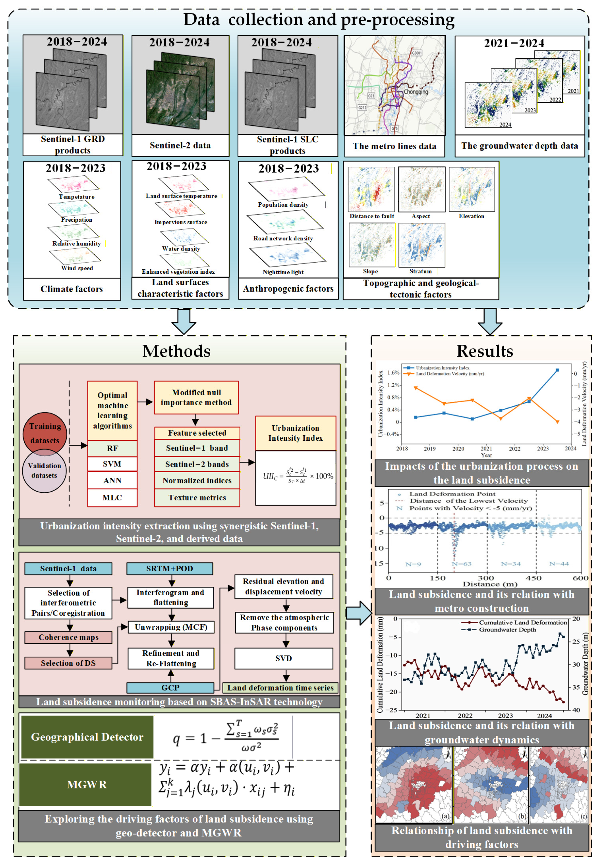
In this study, the combination of GD and MGWR was used to analyze the driving factors of land subsidence. This integrated approach enables a comprehensive analysis that simultaneously accounts for factor interactions and spatial heterogeneity, overcoming the limitations of traditional models [98]. The complex topography and uneven urban development in mountainous urban environments lead to significant spatial variability in land subsidence processes. In this context, applying the GD-MGWR approach helps to better identify the primary driving factors, the interactions among them, and their multi-scale spatial variations [99]. The methodological flowchart of this study is presented in Figure 2.

3.6. Comparative Evaluation of SBAS-InSAR and PS-InSAR in Monitoring Land Subsidence

To evaluate the reliability of the SBAS-InSAR results, the PS-InSAR was employed for cross-validation. The PS-InSAR used the same dataset as the SBAS-InSAR analysis. This method generates differential interferograms, selects stable persistent scatterer candidates based on amplitude and amplitude dispersion, and further refines them using temporal coherence. Finally, the PS-InSAR results are obtained through 3D phase un-wrapping and noise removal. Foroughnia et al. [32] used PS-InSAR to monitor land deformation in Tehran with high accuracy. The PS-InSAR processing workflow in this study is consistent with that described in their research. To assess errors, the coefficient of determination (R2) was calculated, and a linear fitting function was applied to the average deformation rates derived from SBAS-InSAR and PS-InSAR. The R2 was calculated as follows [100]:
R 2     =     1     i   =   1 n ( y i     y i ^ ) 2 i   =   1 n ( y i     y ¯ ) 2 ×   j   =   1 k ( Z j     Z ¯ ) 2 k
where R 2 is the coefficient of determination that quantifies the proportion of variance in the dependent variable predictable from independent variables; n denotes the total number of observations or data points in the dataset; y i represents the actual observed value for the i -th data point; y i ^ is the predicted value for the i -th data point; y ¯ indicates the mean of all observed y values; k is the number of independent variables or predictors in the model; Z j is the value of the j -th predictor variable; Z ¯ is the mean of the Z j values across all observations.

4. Results

4.1. Land Subsidence Under the Context of Urbanization

4.1.1. Assessment of Classification Accuracy for Land Cover Based on the Machine Learning Classifier

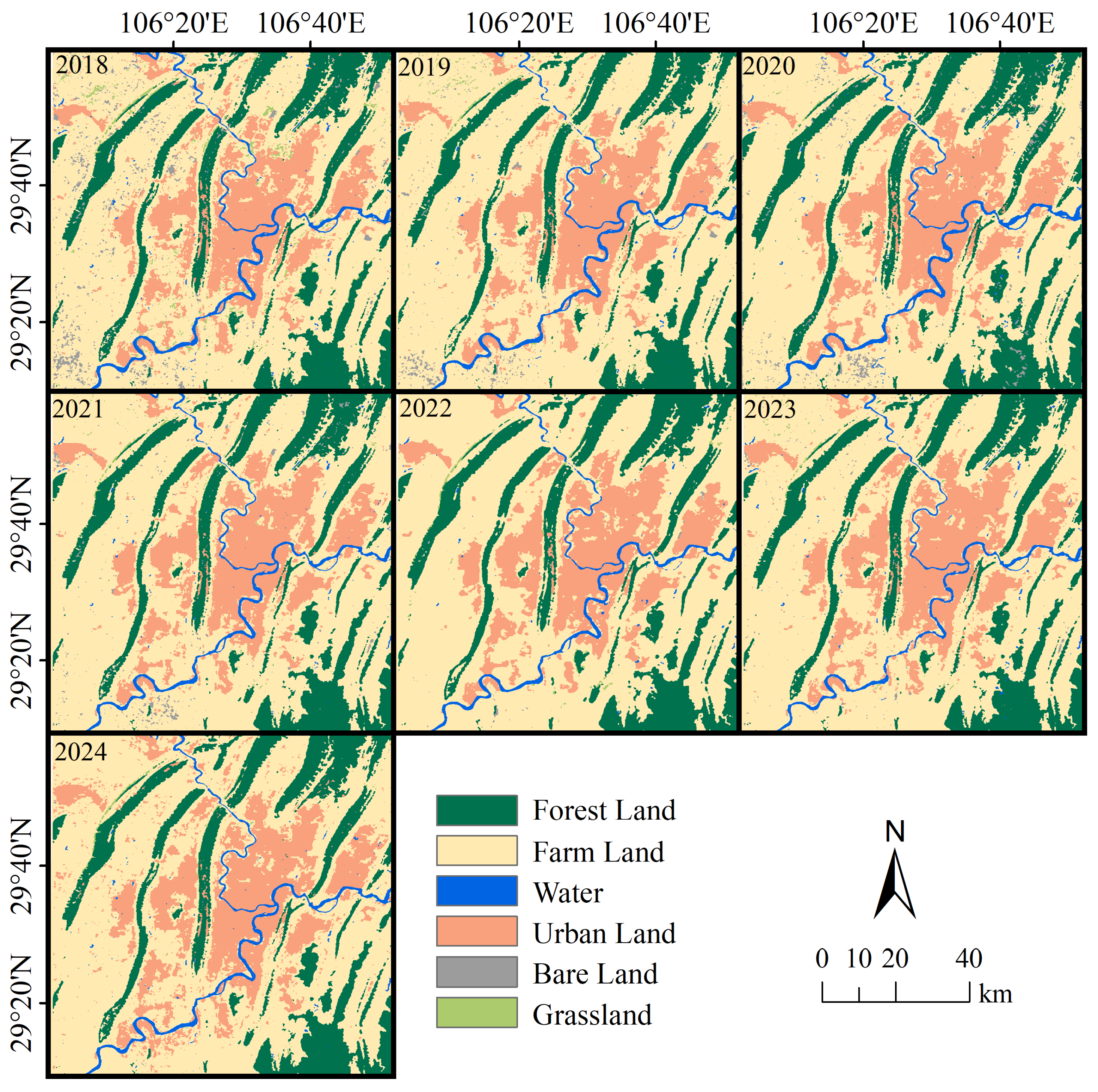
Accuracy comparisons among the machine learning classifiers were performed using 2679 validation data. Based on each classification, overall accuracy, user’s accuracy, kappa index, and producer’s accuracy were averaged to calculate mean accuracy metrics. As shown in Table 6, except for maximum likelihood classification, all classification methods achieved overall accuracy and kappa index values above 0.8. Among these classifiers, the RF algorithm demonstrated the best performance, with both overall accuracy and kappa index reaching 0.88. Support vector machine and artificial neural network took the second and third positions, with overall accuracy values of 0.86 and 0.83, and kappa index of 0.81 and 0.80, respectively. In contrast, maximum likelihood classification generated significantly inferior results, exhibiting the lowest overall accuracy of 0.76 and kappa index of 0.72 among all methods. Based on these findings, this research selected RF as the best-performing machine learning classifier to produce the land classification map of the study area (Figure 3).

4.1.2. The RF Classifier Combined with the Null Importance Feature Selection Method to Extract ISA

As indicated in Table 6, urban land demonstrated comparatively lower classification accuracy than most land cover categories, with user’s accuracy is 0.83 and producer’s accuracy is 0.77. Its kappa index is 0.82 also underperformed relative to other types, though it exceeded bare land. This phenomenon arises from spectral reflectance convergence between urban land and bare land in specific wavelength ranges. For example, low reflectance impervious surface (e.g., asphalt pavement) display spectral characteristics in visible and near-infrared bands of Sentinel-2 data that significantly overlap with bare soil reflectance properties. Consequently, spectral confusion occurs, impeding accurate differentiation of the ISA type in remote sensing imagery. For improving the urban ISA extraction accuracy, Sentinel-1 and Sentinel-2 original bands, SAR and spectral indices features, and texture features were extracted to mitigate misclassification between ISA and spectrally similar land cover types (Table 3). Therefore, feature selection became essential as many of the 35 features could be strongly correlated. Through null importance feature selection method, as shown in Figure 4, retaining 26 features with scores > 0 as the optimal feature combination for impervious surface extraction.
Seven distinct RF classification experiments were designed to validate the efficacy of fusing multi-feature sets with null importance method, employing the following input individual datasets and the combination of different datasets (Table 7).
Notably, combinations of multi-source feature extraction datasets yielded suboptimal accuracy. Combining SAR data with spectral indices and texture features resulted in notably poorer performance, as indicated by an overall accuracy and kappa index both standing at just 0.79. The efficacy of feature selection results was demonstrated through enhanced classification outcomes. Implementing feature selection boosted the overall accuracy from 0.88 to 0.95 and raised the kappa index from 0.87 to 0.94. These findings suggest that with sufficient training data, excessive features may reduce classification accuracy, potentially due to redundancy and low-quality inputs. After applying null importance selection, irrelevant features are removed. This process enhances both computational efficiency and final prediction accuracy. Table 8 displays the confusion matrices distinguishing ISA from non-ISA land cover categories. For the study area, the proposed methodology significantly improved classification performance, achieving an overall accuracy of 0.94 and a kappa index of 0.90, marking an improvement over results from using only the RF classifier.
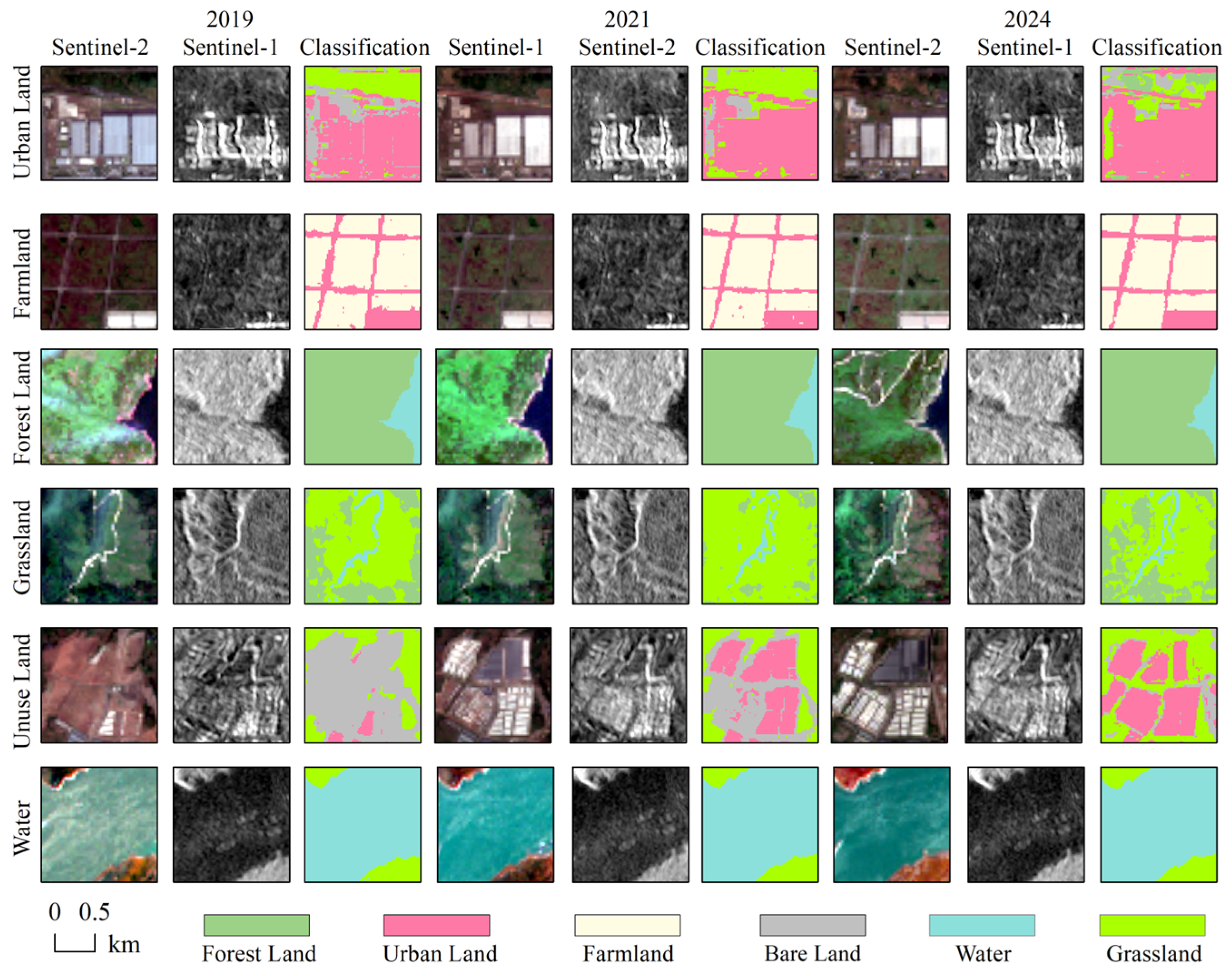
To illustrate the efficacy of the proposed method, Figure 5 displays the land cover classification outcomes, featuring a local close-up view and the extracted ISA. As evident from the results, class boundaries of various land covers are markedly sharper, particularly with road networks and buildings being accurately extracted as impervious surface. This significantly reduced confusion between impervious areas and bare soil and vegetation.

4.1.3. Spatiotemporal Dynamics of Land Subsidence

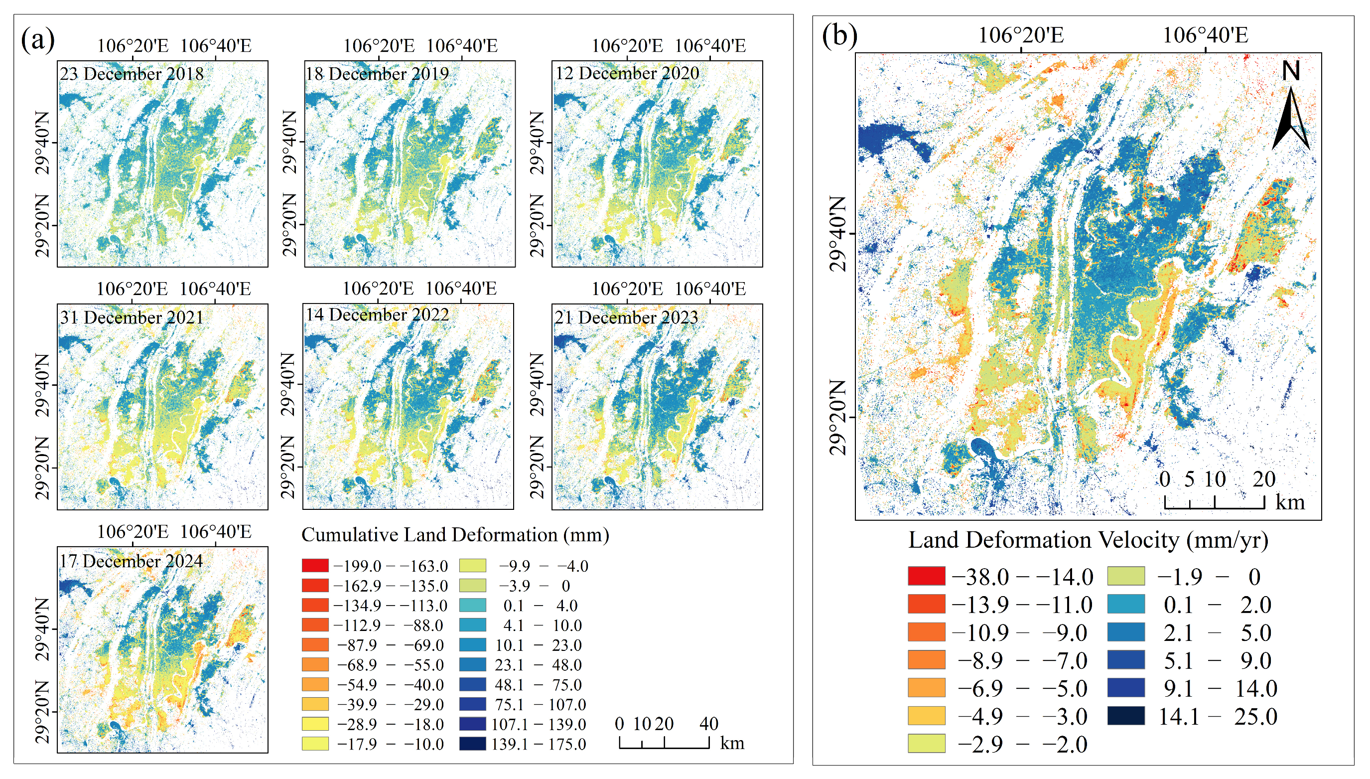
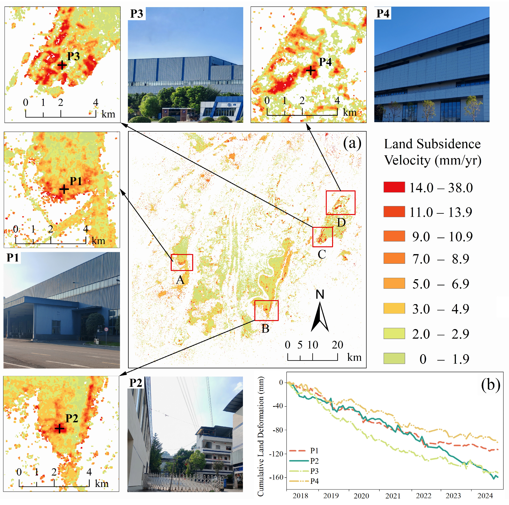
Figure 6 shows the land deformation results along the line of sight. As shown in Figure 6a,b, cumulative land deformation ranged from −199 mm to 175 mm over the study period, with deformation rates between −38 mm/yr and 25 mm/yr. Positive values indicate land uplift, whereas negative values indicate land subsidence. Missing pixels in the results may be caused by the influence of vegetation cover on radar signal coherence [33].
This study extracted the land subsidence component from the land deformation velocity data (Figure 7a). The land subsidence area covered 1160.66 km2, accounting for 15.61% of the entire study area, and concentrated in densely populated urban areas. The maximum overall land subsidence velocity reached 38 mm/yr, and the average land subsidence velocity was 3.3 mm/yr. The monitoring points with land subsidence velocity of 0–10 mm/yr, 10–30 mm/yr, and 30–40 mm/yr accounted for 96.07%, 3.92%, and 0.01%, respectively. According to the Technical Regulations for Land Subsidence Interferometric Radar Data Processing (DD2014-11) issued by the China Geological Survey [101], land subsidence is not very severe in the study area, yet it is more pronounced in localized regions (Table 9).
Land subsidence is predominantly distributed across the western, eastern, and southern parts of the study area. The most pronounced land subsidence occurs in the western zone, where the average velocity reaches 3.97 mm/yr. The most significant land subsidence is observed in subarea A of Bishan District, located within the industrial park near Hujiawan, with an average velocity of 15.12 mm/yr and a range of 0.3–32.9 mm/yr. Following closely, the eastern zone exhibits an average land subsidence velocity of 3.72 mm/yr. Within this zone, land subsidence is mainly concentrated in subarea C of Jiangbei District, located in the Yufu Industrial Development Zone, with an average velocity of 21.38 mm/yr and a range of 1.3–36.3 mm/yr, and in subarea D of Yubei District, situated within the core area of the regional automobile industry cluster, with an average velocity of 17.64 mm/yr and a range of 0.8–37.5 mm/yr. Land subsidence in the southern zone is relatively slight, with an average velocity of 2.98 mm/yr. The most intense land subsidence is found in subarea B of Banan District, covering Liujia Gang, Jiefang Xincun, and their adjacent regions, with an average velocity of 19.31 mm/yr and a range of 0.5–35.7 mm/yr.
To reveal temporal land subsidence trends in significant land subsidence areas, points P1, P2, P3, and P4, with land subsidence velocities in the high category listed in Table 9, were selected from subareas A, B, C, and D for time-series analysis (Figure 7b). The land subsidence velocities at P1, P2, P3, and P4 were 31.8 mm/yr, 34.2 mm/yr, 35.1 mm/yr, and 37.1 mm/yr, respectively. As shown in Figure 7b, the cumulative land subsidence time series indicates that land subsidence increased each year at four points, with total land subsidence reaching 108.91 mm (P1), 162.11 mm (P2), 152.39 mm (P3), and 107.41 mm (P4) by 2024. P1 is situated at an automobile component manufacturing facility. This land subsidence is potentially related to soil compaction from frequent vibrations of large machinery and vehicular loading from logistics operations. P2 is located within an industrial development zone, where the land subsidence observed is likely caused by concentrated heavy machinery loads that exceed the foundation’s bearing capacity. P3 is situated within a major regional automobile manufacturing facility, where long-term industrial groundwater extraction may have led to a decline in the groundwater level and subsequent land subsidence. P4 is located in the core area of the eastern automobile industry, underwent large scale construction during the study period. The observed land subsidence is primarily attributed to prolonged groundwater extraction and changes in soil structure associated with construction activities. An analysis of these four points with significant land subsidence shows that industrial operations have a substantial influence on land subsidence in Chongqing, the leading industrial center of Southwest China.

4.1.4. The Relationship Between Urbanization Intensity and Land Subsidence

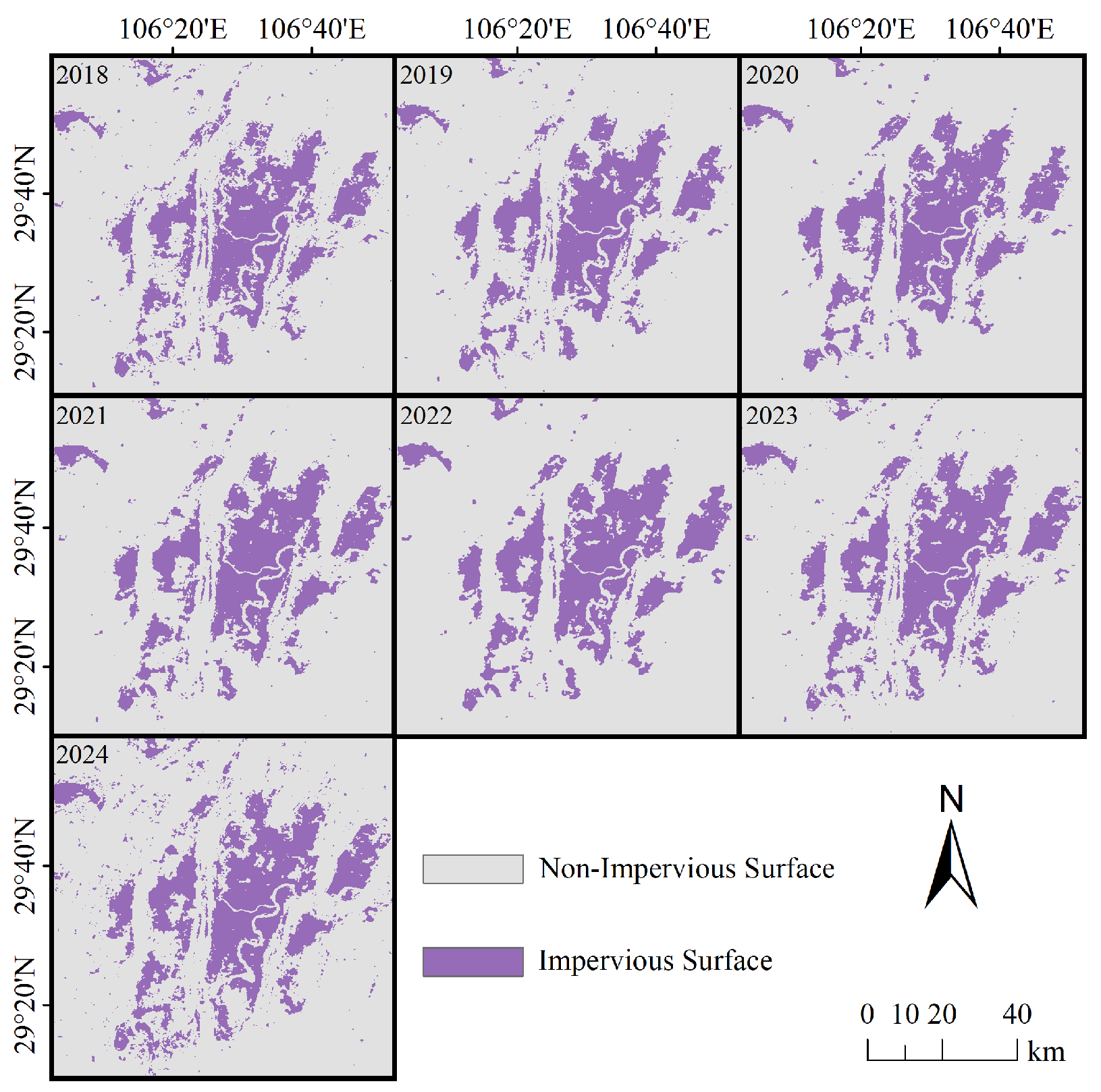
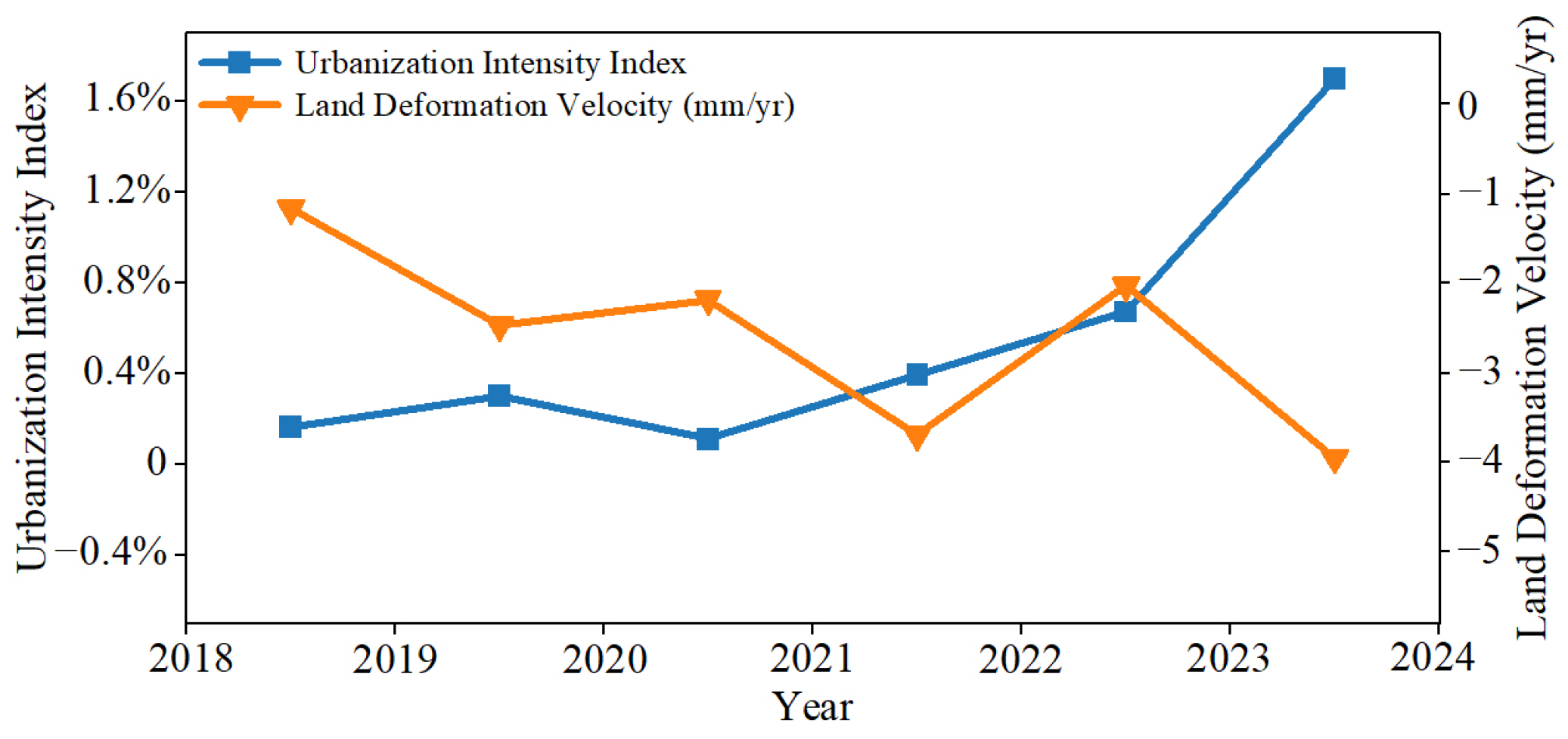
Figure 8 presents the spatial distribution maps of ISA extracted across the study area from 2018 to 2024 using an RF classifier combined with null importance feature selection, along with the resulting UII values calculated directly from the ISA extraction results. The study period shows the same trajectories between urbanization intensity and land subsidence velocity (Figure 9). The UII increased from 0.19% in 2018 to 1.63% in 2024, while land subsidence concurrently intensified from 0.93 mm/yr to 4.12 mm/yr. Two critical patterns emerge: first, high values of land subsidence during UII’s steepest growth phase from 2022 to 2024. Second, despite UII stabilization between 2018 and 2022, land subsidence progression persisted—indicating that beyond urbanization intensity, land subsidence is significantly influenced by multiple complex driving factors.

4.2. Land Subsidence and Its Relation with Metro Construction

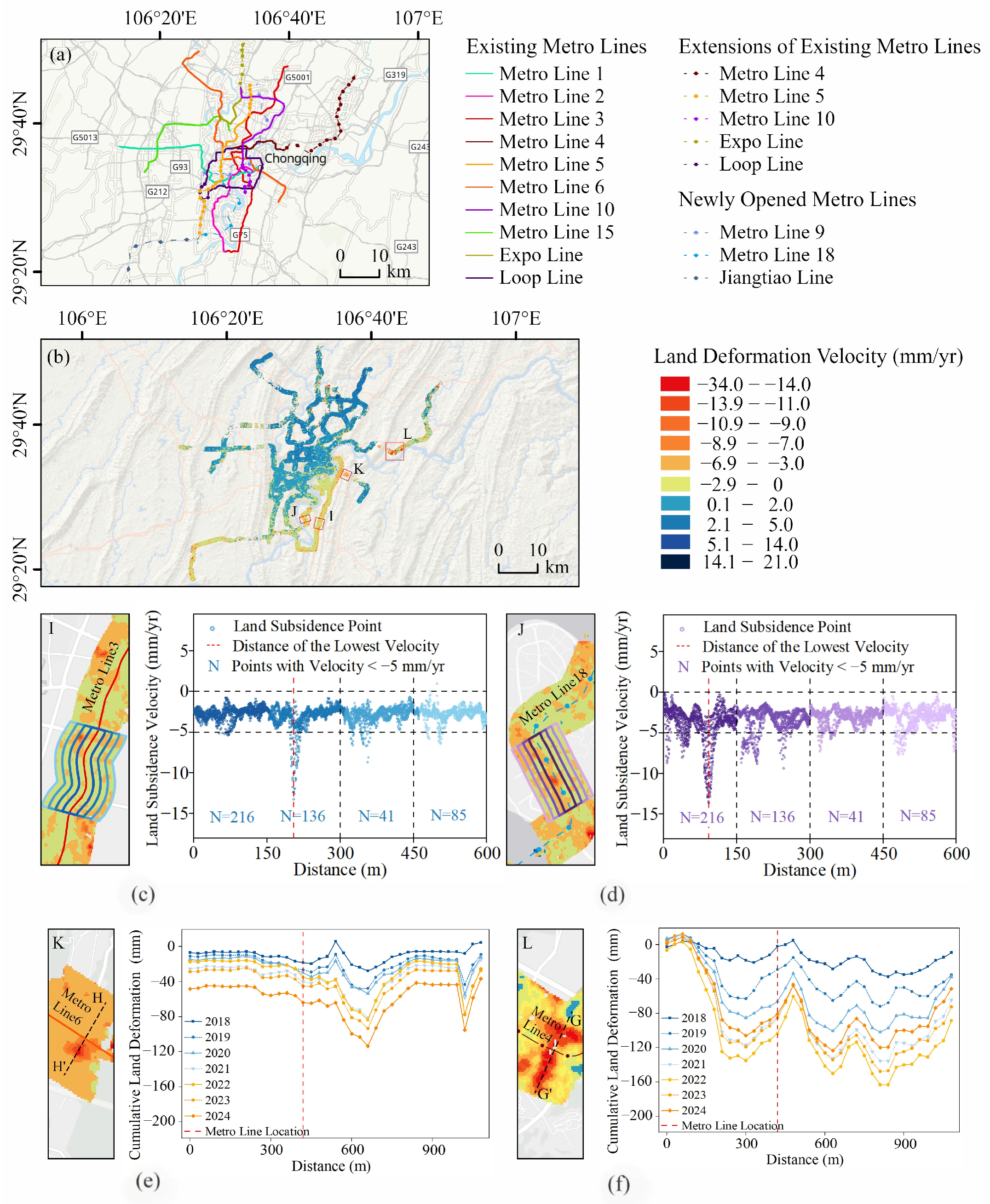
This study examines the impact of constructing and operating metro lines on land subsidence, highlighting the specific land deformation patterns observed along the Chongqing metro network. The specific opening status of metro lines in the study area is shown in Figure 10a. Metro lines inaugurated before 2020 were defined as existing lines, while both newly opened lines and extensions of existing lines opened in 2020 and onward were designated as newly opened lines in this study. This study evaluates the impact of Chongqing metro lines on land subsidence by extracting land deformation data within a 600 m buffer zone [102,103]. As shown in Figure 10b, within the land deformation velocity buffer zones, the area of land subsidence is 207.76 km2, accounting for 42.16% of the buffer zones. Land subsidence along newly opened and existing lines accounted for 55.79% and 44.21% of the total land subsidence area within the buffer zones, respectively. This result indicates that land subsidence was more pronounced along newly opened metro lines compared to existing ones during both metro construction and operation stages. This may be because metro construction disturbance exerts a greater impact on land subsidence than operational vibrations [104,105].
To analyze and compare land subsidence patterns along existing and newly opened metro lines, this study uses four segments with relatively pronounced subsidence: two existing lines comprising metro line 4, Segment I (Dashancun–Chalukou Stations, Figure 10c) and metro line 6, Segment K (Shangxinjie–Liujiaping Stations, Figure 10e); and two newly opened lines containing metro line 18, Segment J (Chongqing University of Technology–Lijiatuo Bridge Stations, Figure 10d) and metro line 4 extension, Segment L (Tieshanping–Luxi Stations, Figure 10f), and longitudinal deformation velocity profiles along cross-sections HH’ of Segment K and GG’ of Segment L were plotted. In Segment I, land subsidence velocities along both sides of metro line primarily ranged within 0–5 mm/yr, indicating localized stability. The maximum land subsidence velocity area occurs 187 m from the metro line, where 63 monitoring points exceeded 5 mm/yr. This area is located in an industrial manufacturing park. The slight land subsidence observed here is likely due to vibrations from heavy industrial machinery, combined with minor groundwater extraction. These factors may cause soil compaction, thereby resulting in land subsidence [106,107,108]. In Segment J, significant land subsidence occurred along both sides of the metro line, with a land subsidence center forming within 150 m of the metro line. A total of 216 monitoring points exhibited land subsidence velocities greater than 5 mm/yr. As there are no other major construction activities in the vicinity, the land subsidence is likely caused by soil disturbance resulting from metro tunnel excavation [109,110]. In Segment K, land subsidence along the profile remained generally stable, except for a pronounced land subsidence center at 200 m from the metro line with 110.5 mm cumulative land subsidence. This land subsidence center was located at a factory engaged in material processing and storage logistics. Construction, groundwater extraction, and pipeline leakage may cause soil consolidation and instability. These were likely the main reasons for the land subsidence at this location [111,112]. In Segment L, noticeable fluctuations in land subsidence were observed along the profile, with two distinct subsidence centers forming within 160 m on both sides of the metro line. Since no other significant construction activities occurred nearby, the underground excavation during metro construction is likely the main factor causing land subsidence [113,114].
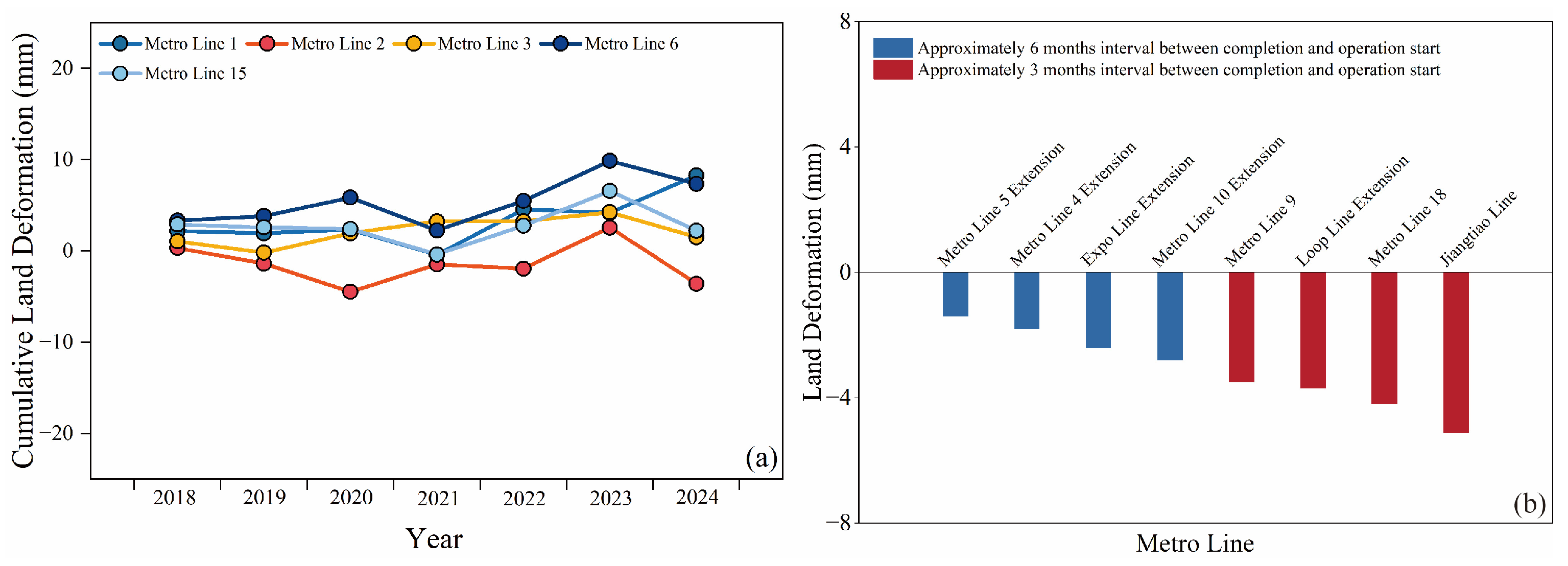
Figure 11a demonstrates that land deformation along the five existing lines remained relatively stable, with values ranging from −8.73 mm to 9.82 mm. To further analyze land deformation trends before and after metro operation, the increase in land subsidence within three months after the opening of the eight newly opened lines was obtained (Figure 11b). Within this period, cumulative land subsidence increased by 1.4 mm, 1.8 mm, 2.4 mm and 2.8 mm, for the Metro Line 5 extension, Metro Line 4 extension, Expo Line extension, and Metro Line 10 extension, respectively, and by 3.5 mm, 3.7 mm, 4.2 mm, and 5.1 mm for the Metro Line 9, Loop Line extension, Metro Line 18, and Jiangtiao Line, respectively. The differences in land subsidence among these metro lines may be related to the interval between construction completion and the start of operation. For intervals longer than six months, land subsidence after metro operation was relatively minor, whereas for intervals shorter than three months, land subsidence increased more significantly after metro operation. This phenomenon is likely due to soil consolidation. When the interval between construction completion and operation is short, the soil has not yet fully consolidated under the primary static load of the metro infrastructure itself, and the dynamic load generated by train operation is applied to the soil, leading to additional land subsidence [115]. Conversely, when the interval is long, most of the consolidation has been completed before operation. Therefore, the additional land subsidence caused by the subsequent dynamic train load is relatively small.

4.3. Land Subsidence and Its Relation with Groundwater Dynamics

Previous studies demonstrate that when groundwater’s supporting effect diminishes, pore water pressure shifts to the soil skeleton, inducing soil consolidation and land subsidence [116,117,118]. Groundwater level refers to the position of the water table relative to a reference plane, while groundwater depth is the vertical distance from the ground surface to the groundwater level. In this study, the High Accuracy Surface Modeling (HASM) method [119,120] was applied to generate spatiotemporal maps of groundwater depth variations across the study area for the period 2021–2024 (Figure 12a). During this period, groundwater depth decreased from 30.65 m to 23.93 m, corresponding to an overall rise in groundwater level of 6.72 m. Specifically, areas with relatively low groundwater levels were mainly concentrated in the eastern, western, and southern parts of the study area. Figure 12b shows a declining trend in groundwater levels from June 2022 to June 2023, with groundwater depths peaking at 34.24 m and 34.81 m. The variations in groundwater levels during this period correspond closely with the observed trends in land subsidence. This phenomenon is primarily attributed to Chongqing experiencing severe heat events, significantly reduced precipitation, and severe drought conditions in 2022. During the summer of 2022, the region recorded notably higher average temperatures and lower precipitation compared to other years (Figure 12c). From June 2022 to June 2023, persistent region-wide high temperatures and heat impacts contributed to declining groundwater levels, thereby inducing land subsidence [121,122,123]. Beyond this period, however, only a weak correlation was observed between groundwater fluctuations and land subsidence trends, indicating that other factors likely dominated subsidence dynamics. Consequently, while groundwater level variations significantly influenced subsidence during distinct intervals, they cannot be considered the primary driver across Chongqing’s mainly urban area.

4.4. Relationship of Land Subsidence with Driving Factors in Chongqing

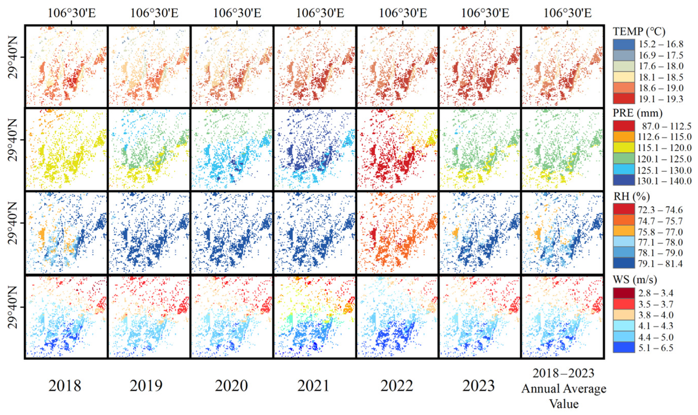
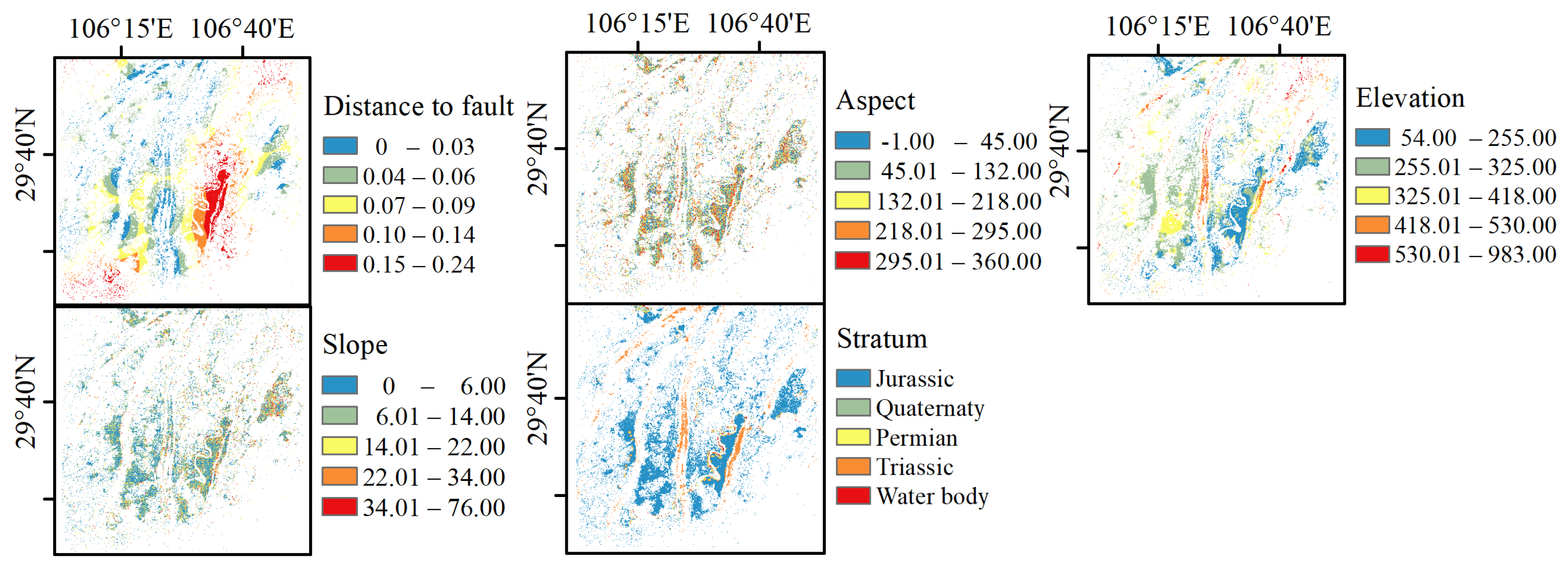
The spatial distributions of the selected anthropogenic, climatic, and land surface characteristic factors are presented in Figure 13, Figure 14, Figure 15 and Figure 16. Each driving factor was extracted based on the land subsidence zones identified in the deformation rate map of the study area and resampled to match the spatial resolution of the land subsidence velocity data to facilitate the GD analysis.

4.4.1. The Influence of Potential Driving Factors on Land Subsidence

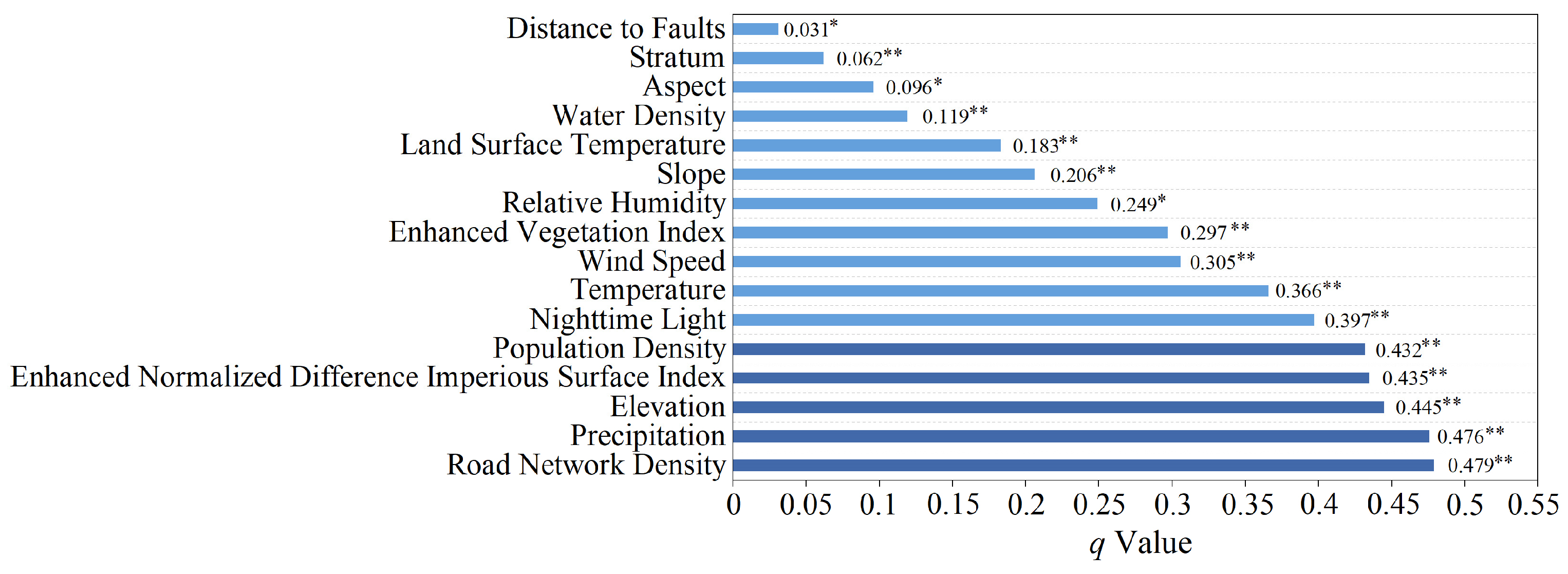
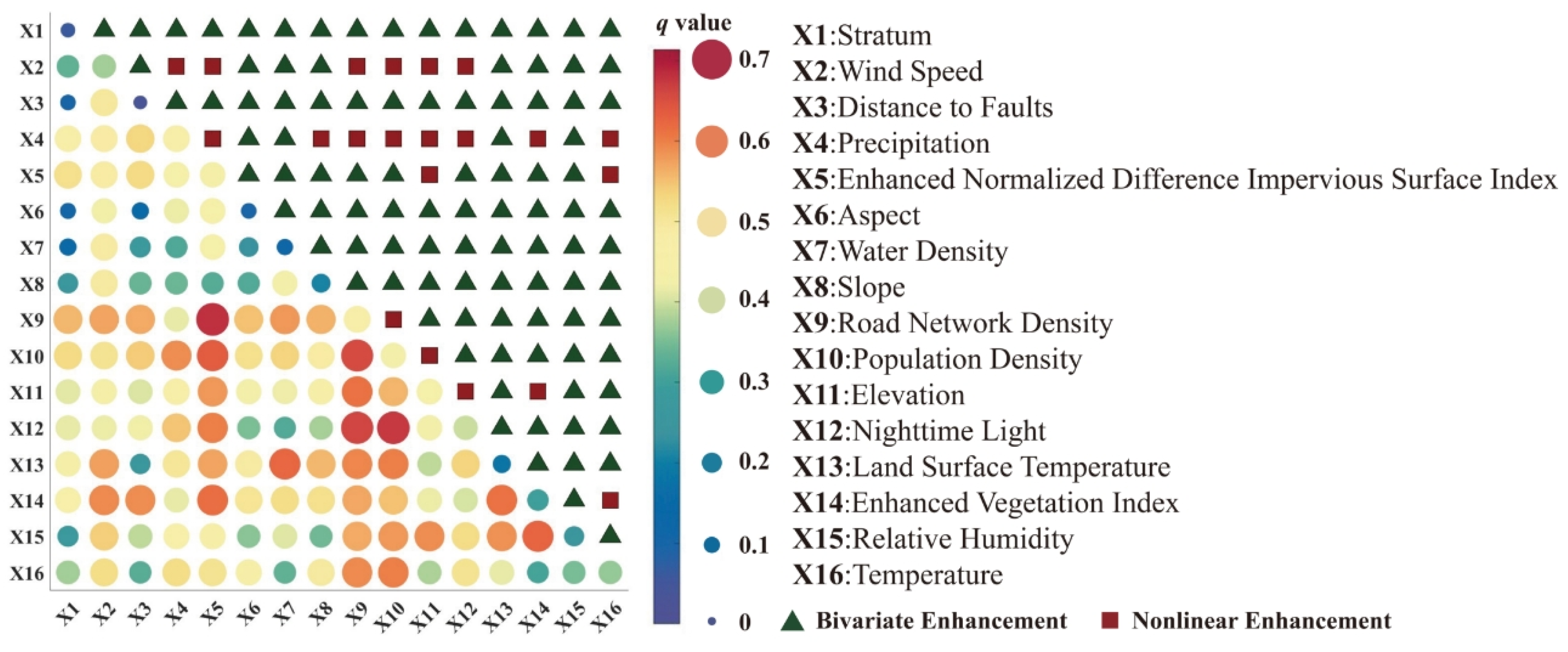
Figure 17 shows the influence (q values) of the driving factors on land subsidence as calculated by the GD model. The anthropogenic factors are the most prominent factors, such as RND (q= 0.479), PD (q= 0.432), and NTL (q= 0.397) had more greater influence on the pattern of land subsidence, with the strength of correlation declining from climate factors > land surface characteristic factors > topographic and geological-tectonic factors.

4.4.2. Interactions Between Different Driving Factors

Figure 18 displays the q-values of both individual factors and their interactions, all of which exhibit statistical significance, as confirmed by p-values less than 0.01. The results indicate that interactions between factors exhibit both bivariate and nonlinear enhancements. Remarkably, when comparing the effects of each factor pair, those involving road network density exhibit more significant explanatory power. The combinations of factors that exhibited the highest explanatory power are road network density ∩ enhanced normalized difference impervious surface index (0.682), road network density ∩ nighttime lights (0.664), and road network density ∩ population density (0.657). With regard to interaction structure, the interaction of population density with nighttime lights (0.654), population density with enhanced normalized difference impervious surface index (0.635), enhanced vegetation index with enhanced normalized difference impervious surface index (0.615), and enhanced normalized difference impervious surface index with nighttime lights (0.601) exhibits the strongest levels of influence. In summary, the interaction between anthropogenic factors and land surface characteristic factors exerts the most significant effect on land subsidence.

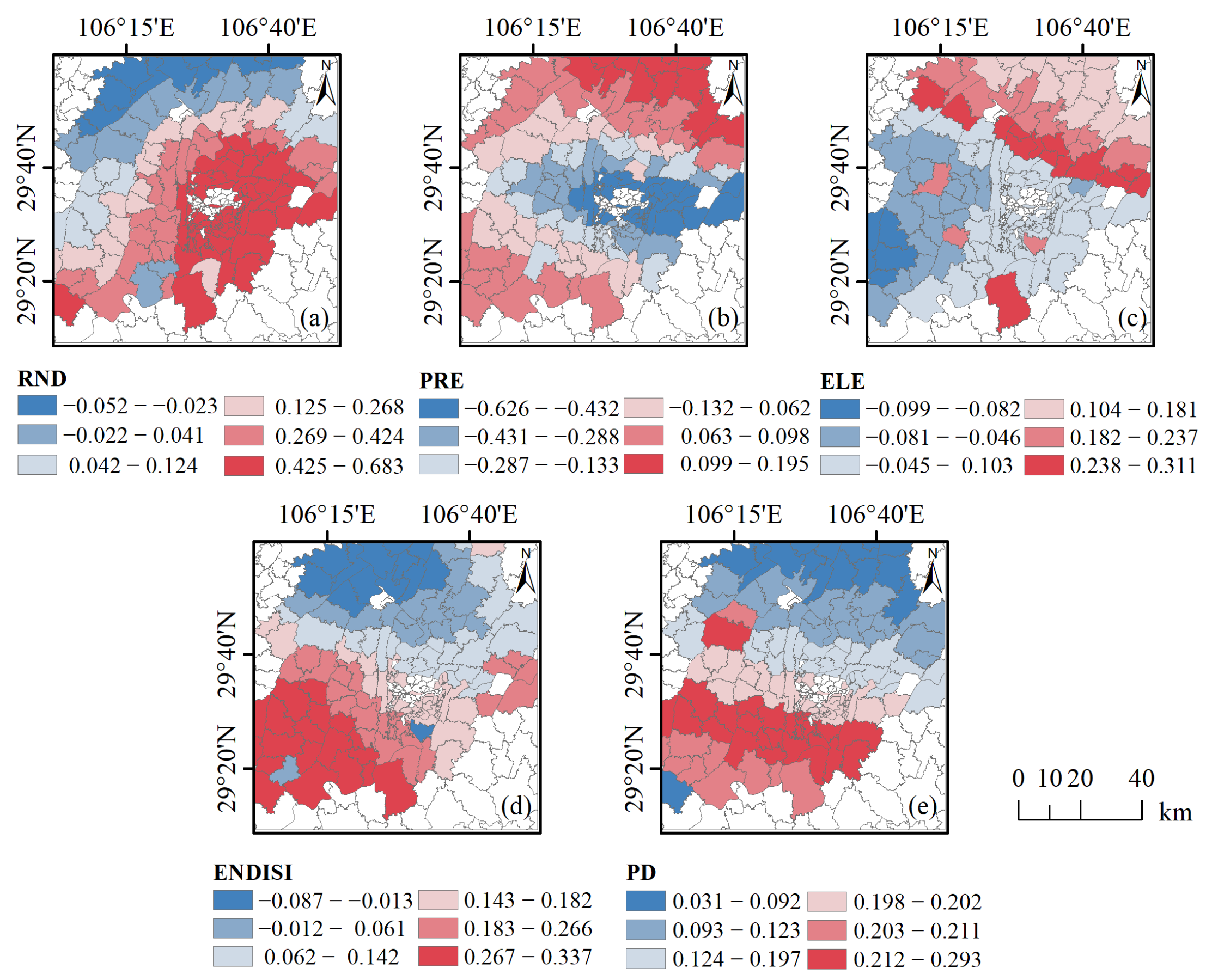
4.4.3. Spatial Pattern Analysis of Regression Coefficient

Urban planning units are regional subsystems formed through either autonomous urban development or formal planning. They also serve as the basic units for implementing land use, shaping the spatial environment, and conducting planning evaluations [124]. To more accurately reflect the spatial variations in the main driving factors of land subsidence, urban planning units were selected as the analysis units. The MGWR model was used to analyze the spatial distribution patterns of the effects of these main driving factors on land subsidence. The blank areas in Figure 19 correspond to regions where no land subsidence was detected or where pixels were missing in the SBAS-InSAR results. Therefore, these areas were excluded from the analysis of land subsidence driving factors during the MGWR modeling.
As shown in Figure 19a, road network density shows a clear positive correlation with land subsidence in the southeastern part of the study area. This is because the area is the city’s commercial core, serving as a major hub for commerce and finance in western China, with relatively high road density [125]. As shown in Figure 19b, precipitation exhibits a negative correlation with land subsidence across most of the main urban districts in the study area, which is likely due to increased precipitation raising groundwater levels, thereby mitigating the occurrence of land subsidence. As shown in Figure 19c, the correlation between elevation and land subsidence is weak, mainly observed in the relatively low-elevation areas of the main urban region, indicating that in Chongqing’s complex topography, elevation has little direct influence on land subsidence. As shown in Figure 19d, the enhanced normalized difference impervious surface index exhibits a positive correlation with land subsidence and shows spatial consistency with population density (Figure 19e), primarily in the southern part of the study area. This is mainly attributable to this region being a major industrial manufacturing zone in Chongqing, where the average industrial gross domestic production from 2018 to 2023 accounts for approximately 45.7% of the study area, accompanied by relatively high proportions of impervious surfaces and population density.

5. Discussion

5.1. Accuracy Verification of SBAS-InSAR in Monitoring Land Subsidence

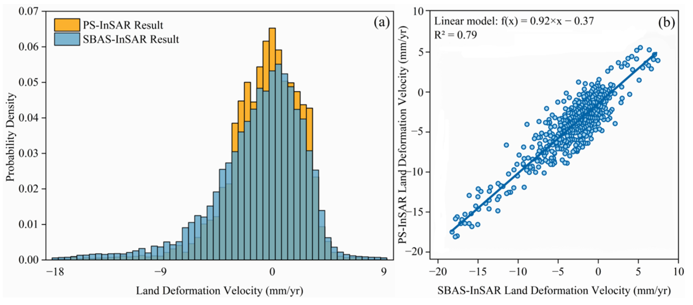
This study employed the SBAS-InSAR to monitor long-term land subsidence in Chongqing, a typical mountainous city. This technique enables continuous, large-scale land deformation monitoring, making it applicable for assessing land subsidence of buildings [126], as well as critical infrastructure such as long-span bridges [127] and highways [128]. Nevertheless, the technique has inherent limitations. Higher-resolution SAR images can exacerbate foreshortening, layover, and shadow effects in densely built areas, thereby adversely affecting the derived time-series deformation results [129]. While validation of SBAS-InSAR results with contemporaneous leveling and borehole data is considered relatively reliable [130,131], this study’s validation approach was constrained by the lack of such data. Consequently, the PS-InSAR served as the validation method for assessing the reliability of the SBAS-InSAR results. Teng et al. [132] cross-validated SBAS-InSAR-derived urban land deformation results in Hefei using PS-InSAR and found that, despite minor algorithmic discrepancies, both techniques exhibited consistent land deformation trends, thereby confirming the reliability of the SBAS-InSAR method. Xu et al. [133] utilized SBAS-InSAR to characterize land subsidence spatiotemporal patterns in Lanzhou, with cross-validation against PS-InSAR revealing high consistency, with a mean error of 1.51 mm/yr. Li et al. [42] demonstrated that SBAS-InSAR achieves accurate land subsidence inversion in Tianjin, with PS-InSAR results directly validating SBAS-InSAR outcomes (R = 0.974), confirming cross-validation consistency. Therefore, the SBAS-InSAR results were validated through cross-validation with the PS-InSAR in this study (Figure 20).
Given that sparse PS-InSAR points in densely vegetated or steeply sloped areas lead to uneven spatial coverage and validation results skewed toward urban or bare rock surfaces [34,134], the central urban districts of Jiulongpo, Dadukou, Jiangbei, and Yuzhong were therefore strategically selected as validation areas to more accurately assess SBAS-InSAR results (Figure 1b). A probability density analysis of land deformation velocities was performed using 979,078 slow decoherence filtering phase points from SBAS-InSAR and 1,013,251 permanent scatterer points from PS-InSAR. As shown in Figure 20a, the land deformation velocity distributions obtained from PS-InSAR and SBAS-InSAR are similar, with most values concentrated between –4 mm/yr and 3.5 mm/yr. The probability distributions of identical land deformation velocities are also similar, indicating strong consistency between the two methods in monitoring land deformation. To further confirm the reliability of the SBAS-InSAR results, linear regression was performed on land deformation points with identical coordinates obtained from both PS-InSAR and SBAS-InSAR results (Figure 20b). The findings reveal R2 = 0.79, demonstrating a strong correlation between the two methods. These validation findings confirm the reliability of the SBAS-InSAR results in this study.
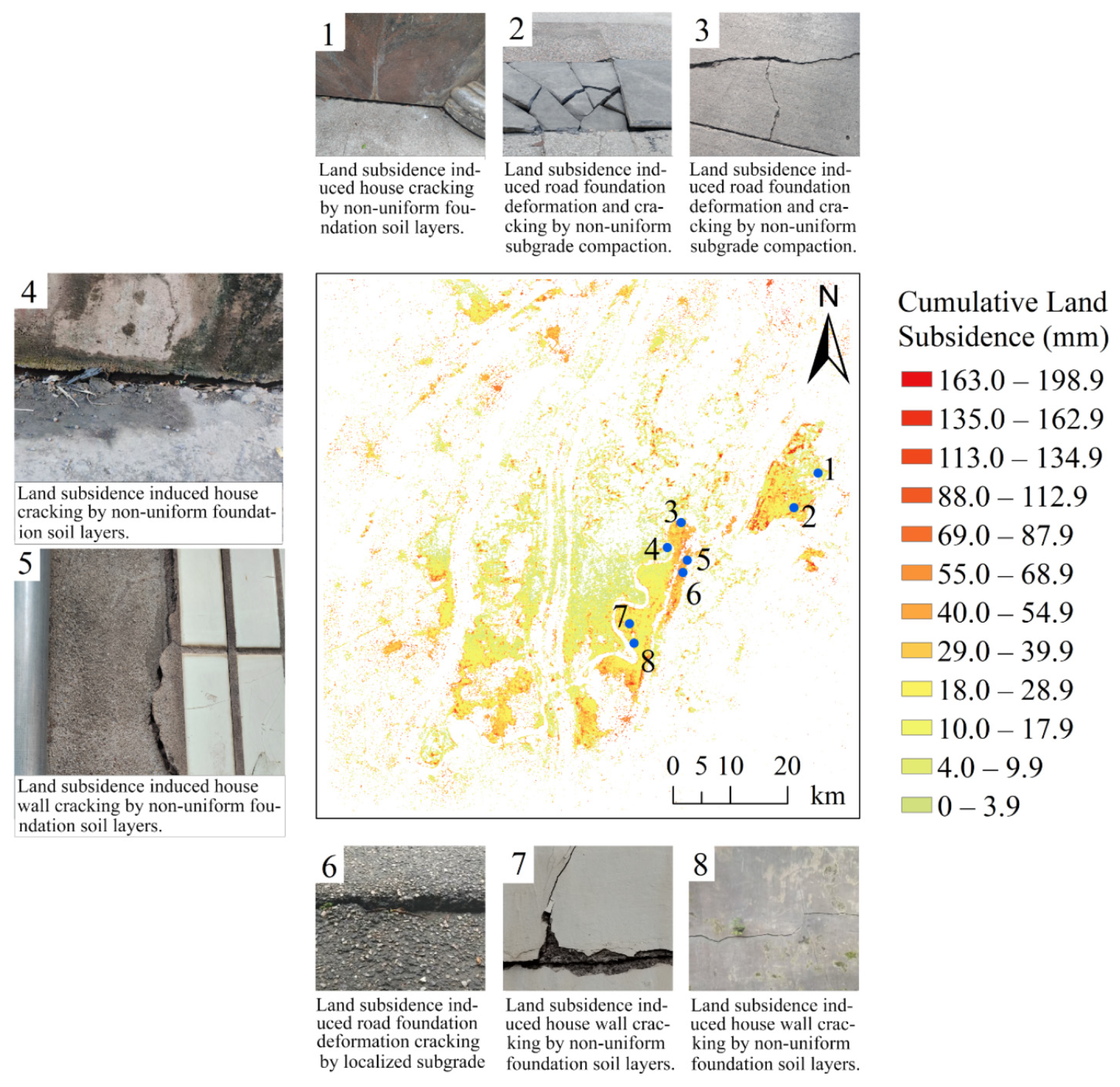
Based on the official land subsidence observation records provided by the Chongqing Authorities, field verification was conducted in Jiangbei, Yubei, Nan’an, Yuzhong, and Banan districts during 2025. Photographs and coordinate information were collected for areas where land subsidence had not been timely addressed. As shown in Figure 21, the coordinates of points 1 to 8 were compared with the cumulative land subsidence areas obtained from the SBAS-InSAR results in 2024. The comparison indicates that all points are located within the cumulative land subsidence areas. Among them, points 2, 4, 6, and 7 show larger cumulative land subsidence values, while points 1, 3, 5, and 8 exhibit smaller values. These findings are consistent with the results of field observations, demonstrating that the SBAS-InSAR results agree with the on-site measurements and providing empirical support for the reliability of the study results.

5.2. Limitations and Future Work

Firstly, the application of SBAS-InSAR for land subsidence monitoring in this study yielded satisfactory results. However, according to the general survey results released by the Chongqing Municipal Planning and Natural Resources Bureau, over 90% of the terrain in the main urban area of Chongqing consists of mountains and hills. The area also has relatively high vegetation coverage, which can compromise radar phase stability and reduce the reliability of deformation monitoring. Limited canopy penetration causes radar waves to scatter primarily aboveground, preventing the detection of subsurface deformation [129,135]. Therefore, further refinements are possible in the InSAR technology. For example, Zhang et al. [136] present a hybrid land subsidence monitoring approach that strategically fuses PS-InSAR and SBAS-InSAR, adapting to areas with distinct radar scattering characteristics. Hu et al. [19] monitored land subsidence in a coastal urban area using an integrated approach that combined SBAS-InSAR and global navigation satellite system technologies. Furthermore, future research should collect leveling survey data to facilitate the validation and calibration of SBAS-InSAR-based subsidence monitoring methodologies.
Secondly, this study investigated and discussed the driving factors behind urban land subsidence. The previous literature suggests that urban land subsidence is driven by the synergistic interaction between static drivers [137,138], such as topographic and geological-tectonic factors, and dynamic drivers [139], including climate factors and land surface characteristic factors. Topographic and geological-tectonic factors exhibit minimal changes over the past 20 years. Consequently, this study treats topographic and geological-tectonic factors as static drivers. Static driving data from a single time period is used, and the time-lag effect of these data is neglected. These static driving data are then analyzed alongside dynamic drivers. This may lead to an underestimation of the contribution from the static driver. Therefore, addressing the issue of mixed temporal resolutions remains a challenge and a key focus for future research in land subsidence driver analysis.
Thirdly, the availability of C-band InSAR data for subsidence analysis is well established, with continuous temporal coverage from the 1990s to the present provided by missions such as ERS-1/2, Radarsat-2, and Sentinel-1. This facilitates long-term monitoring. However, while groundwater dynamics are a recognized primary driver of urban land subsidence [140], the analysis in this study was constrained by the limited temporal scope of the available groundwater depth data. Therefore, to enable a more comprehensive understanding of the land subsidence process, it is crucial to enhance the collection of historical groundwater records and conduct longer-term analyses the relationship between land subsidence and groundwater dynamics.

6. Conclusions

Chongqing, acclaimed as the world’s largest mountain city with over 75% mountainous terrain, serves as a typical example for analyzing land subsidence in mountainous urban areas. Land subsidence in Chongqing covered 1160.66 km2 and the average land subsidence velocity was 3.3 mm/yr. Land subsidence is predominantly clustered in the western, eastern, and southern urban areas, especially industrial zones, where the maximum land subsidence velocity reached 38 mm/yr. Anthropogenic factors exert the strongest influence on subsidence. The top six drivers, ranked by explanatory power, are road network density, precipitation, elevation, enhanced normalized difference impervious surface index, population density, and nighttime light. During the extreme high-temperature period in 2022–2023, groundwater levels dropped sharply, correlating with a peak cumulative subsidence. Beyond this period, groundwater played a minor role, indicating the dominance of other factors. Within the timeframe of this study, newly opened metro lines experienced more pronounced land subsidence than existing lines, accounting for 55.79% of the total land subsidence area within the buffer zones, likely due to the impact of metro construction. Shorter intervals between construction completion and operation were also associated with greater land subsidence during the first three months, which may be attributed to soil consolidation.
To effectively combat urban land subsidence in Chongqing, the recommendations derived from this study’s analysis include: (1) government departments should establish and improve the land subsidence monitoring network in Chongqing, with a particular focus on conducting long-term remote sensing monitoring in industrial parks experiencing severe land subsidence. (2) Under the extremely high temperatures, intensified monitoring of groundwater level fluctuations must be implemented; additionally, detailed planning formulation and groundwater extraction activities within land subsidence areas require land subsidence risk evaluations to inform control measures. (3) During metro line construction and throughout operational phases, comprehensive risk evaluations for land subsidence must be conducted to guide regional land subsidence control strategies.

Supplementary Materials

Classification samples can be downloaded at: https://www.mdpi.com/article/10.3390/rs17213539/s1. This material describes all sample data coordinates used for land cover classification mentioned in Table 4.

Author Contributions

Y.L. and Y.Y. jointly conceptualized the research and developed the methodological framework. Y.L. performed the SBAS-InSAR processing. Y.Y. performed urban impervious surface mapping and analyzed urban expansion. Y.L. and J.R. were responsible for the GD and MGWR analyses. Y.L. and Y.D. conducted an analysis of the impacts of metro line construction and groundwater fluctuations on land subsidence. Validation efforts were contributed by Y.L., Y.Y. and K.D. The satellite data were collected and processed by Y.L. and Y.Y. Other driving factor data were collected and processed by Y.L. The draft was written by Y.L. and Y.Y. All authors have read and agreed to the published version of the manuscript.

Funding

This research was funded by the Sichuan Province Science Fund for Distinguished Young Scholars (2023NSFSC1909), the National Earth Observation Data Center Foundation in 2021, grant number of NODAOP2021009.

Institutional Review Board Statement

Not applicable.

Informed Consent Statement

This does not apply.

Data Availability Statement

The sample data used for land cover classification in this study are provided in the Supplementary Materials. Further inquiries can be directed to the corresponding author.

Acknowledgments

The authors sincerely thank the anonymous reviewers for their valuable insights and constructive suggestions. They also gratefully acknowledge the Chongqing General Station of Geological Environment Monitoring for providing the groundwater depth data.

Conflicts of Interest

The authors state that there are no conflicts of interest.

References

  1. United Nations. World Economic and Social Survey 2004; UN: New York, NY, USA, 2004. [Google Scholar]
  2. Shi, L.; Gong, H.; Chen, B.; Zhou, C. Land subsidence prediction induced by multiple factors using machine learning method. Remote Sens. 2020, 12, 4044. [Google Scholar] [CrossRef]
  3. Liu, F.; Zhang, Z.; Zhao, X.; Liu, B.; Wang, X.; Yi, L.; Zuo, L.; Xu, J.; Hu, S.; Sun, F. Urban expansion of China from the 1970s to 2020 based on remote sensing technology. Chin. Geogr. Sci. 2021, 31, 765–781. [Google Scholar] [CrossRef]
  4. Deuskar, C.; Baker, J.L.; Mason, D. East Asia’s Changing Urban Landscape: Measuring a Decade of Spatial Growth; World Bank Publications: Washington, DC, USA, 2015. [Google Scholar]
  5. Wen, H.; Huang, J.; Qian, L.; Li, Z.; Zhang, Y.; Zhang, J. The spatial-temporal evolution patterns of landslide-oriented resilience in mountainous city: A case study of Chongqing, China. J. Environ. Manag. 2024, 370, 122963. [Google Scholar] [CrossRef] [PubMed]
  6. Li, Y.; Gao, J.; Yin, J.; Liu, L.; Zhang, C.; Wu, S. Flood risk assessment of areas under urbanization in Chongqing, China, by integrating multi-Models. Remote Sens. 2024, 16, 219. [Google Scholar] [CrossRef]
  7. Zhang, J.; Tao, Y.; Kou, P.; Jin, Z.; Huang, Y.; Cui, J.; Liang, W.; Liu, R. Dual impacts of urbanization and precipitation on subsidence in Chongqing revealed by SBAS-InSAR. Environ. Earth Sci. 2025, 84, 204. [Google Scholar] [CrossRef]
  8. Xu, Y.S.; Ma, L.; Du, Y.J.; Shen, S.L. Analysis of urbanisation-induced land subsidence in Shanghai. Nat. Hazards 2012, 63, 1255–1267. [Google Scholar] [CrossRef]
  9. Yang, Q.; Ke, Y.; Zhang, D.; Chen, B.; Gong, H.; Lv, M.; Zhu, L.; Li, X. Multi-scale analysis of the relationship between land subsidence and buildings: A case study in an eastern Beijing Urban Area using the PS-InSAR technique. Remote Sens. 2018, 10, 1006. [Google Scholar] [CrossRef]
  10. Ohenhen, L.O.; Shirzaei, M. Land Subsidence Hazard and Building Collapse Risk in the Coastal City of Lagos, West Arica. Earths Future 2022, 10, e2022EF003219. [Google Scholar] [CrossRef]
  11. Haghshenas Haghighi, M.; Motagh, M. Uncovering the impacts of depleting aquifers: A remote sensing analysis of land subsidence in Iran. Sci. Adv. 2024, 10, eadk3039. [Google Scholar] [CrossRef] [PubMed]
  12. Ashraf, T.; Yin, F.; Liu, L.; Zhang, Q. Land Subsidence Detection Using SBAS-and Stacking-InSAR with Zonal Statistics and Topographic Correlations in Lakhra Coal Mines, Pakistan. Remote Sens. 2024, 16, 3815. [Google Scholar] [CrossRef]
  13. Ohenhen, L.O.; Zhai, G.; Lucy, J.; Werth, S.; Carlson, G.; Khorrami, M.; Onyike, F.; Sadhasivam, N.; Tiwari, A.; Ghobadi-Far, K.; et al. Land subsidence risk to infrastructure in US metropolises. Nat. Cities 2025, 2, 543–554. [Google Scholar] [CrossRef]
  14. Zeng, J.; Dai, Z.; Luo, X.; Jiao, W.; Yang, Z.; Li, Z.; Zhang, N.; Xiong, Q. Deformation and Failure Mechanism of Bedding Rock Landslides Based on Stability Analysis and Kinematics Characteristics: A Case Study of the Xing’an Village Landslide, Chongqing. Water 2025, 17, 767. [Google Scholar] [CrossRef]
  15. She, X.; Li, D.; Yang, S.; Xie, X.; Sun, Y.; Zhao, W. Landslide hazard assessment for Wanzhou considering the correlation of rainfall and surface deformation. Remote Sens. 2024, 16, 1587. [Google Scholar] [CrossRef]
  16. Peng, J.; Sun, X.; Wang, W.; Sun, G. Characteristics of land subsidence, earth fissures and related disaster chain effects with respect to urban hazards in Xi’an, China. Environ. Earth Sci. 2016, 75, 1190. [Google Scholar] [CrossRef]
  17. Jung, H.C.; Kim, S.W.; Jung, H.S.; Min, K.D.; Won, J.S. Satellite observation of coal mining subsidence by persistent scatterer analysis. Eng. Geol. 2007, 92, 1–13. [Google Scholar] [CrossRef]
  18. Montenbruck, O.; Steigenberger, P.; Prange, L.; Deng, Z.; Zhao, Q.; Perosanz, F.; Romero, I.; Noll, C.; Stürze, A.; Weber, G. The Multi-GNSS Experiment (MGEX) of the International GNSS Service (IGS)—Achievements, prospects and challenges. Adv. Space Res. 2017, 59, 1671–1697. [Google Scholar] [CrossRef]
  19. Hu, B.; Chen, J.; Zhang, X. Monitoring the land subsidence area in a coastal urban area with InSAR and GNSS. Sensors 2019, 19, 3181. [Google Scholar] [CrossRef] [PubMed]
  20. Chaussard, E.; Amelung, F.; Abidin, H.; Hong, S.H. Sinking cities in Indonesia: ALOS PALSAR detects rapid subsidence due to groundwater and gas extraction. Remote Sens. Environ. 2013, 128, 150–161. [Google Scholar] [CrossRef]
  21. Wang, B.; Zhao, C.; Zhang, Q.; Peng, M. Sequential InSAR time series deformation monitoring of land subsidence and rebound in Xi’an, China. Remote Sens. 2019, 11, 2854. [Google Scholar] [CrossRef]
  22. Du, Y.; Feng, G.; Liu, L.; Fu, H.; Peng, X.; Wen, D. Understanding land subsidence along the coastal areas of Guangdong, China, by analyzing multi-track MTInSAR data. Remote Sens. 2020, 12, 299. [Google Scholar] [CrossRef]
  23. Mohamadi, B.; Balz, T.; Younes, A. A model for complex subsidence causality interpretation based on PS-InSAR cross-heading orbits analysis. Remote Sens. 2019, 11, 2014. [Google Scholar] [CrossRef]
  24. Lin, C.H.; Liu, D.; Liu, G. Landslide detection in La Paz City (Bolivia) based on time series analysis of InSAR data. Int. J. Remote Sens. 2019, 40, 6775–6795. [Google Scholar]
  25. Mohamadi, B.; Balz, T.; Younes, A.J. Towards a PS-InSAR based prediction model for building collapse: Spatiotemporal patterns of vertical surface motion in collapsed building areas—Case study of Alexandria, Egypt. Remote Sens. 2020, 12, 3307. [Google Scholar] [CrossRef]
  26. Mohamadi, B.; Abu Ghazala, M.O.; Li, H.; Al-Sabbagh, T.A.; Younes, A. Integrating InSAR Coherence and Air Pollution Detection Satellites to Study the Impact of War on Air Quality. Int. J. Appl. Earth Obs. Geoinf. 2025, 142, 104687. [Google Scholar] [CrossRef]
  27. Gabriel, A.K.; Goldstein, R.M. Crossed orbit interferometry: Theory and experimental results from SIR-B. Int. J. Remote Sens. 1988, 9, 857–872. [Google Scholar] [CrossRef]
  28. Cigna, F.; Banks, V.J.; Donald, A.W.; Donohue, S.; Graham, C.; Hughes, D.; McKinley, J.M.; Parker, K. Mapping ground instability in areas of geotechnical infrastructure using satellite InSAR and Small UAV surveying: A case study in Northern Ireland. Geosciences 2017, 7, 51. [Google Scholar] [CrossRef]
  29. Hooper, A. A multi-temporal InSAR method incorporating both persistent scatterer and small baseline approaches. Geophys. Res. Lett. 2008, 35, L16302. [Google Scholar] [CrossRef]
  30. Yang, Z.; Li, Z.; Zhu, J.; Wang, Y.; Wu, L. Use of SAR/InSAR in Mining Deformation Monitoring, Parameter Inversion, and Forward Predictions: A Review. IEEE Geosci. Remote Sens. Mag. 2020, 8, 71–90. [Google Scholar] [CrossRef]
  31. Khan, J.; Ren, X.; Hussain, M.A.; Jan, M.Q. Monitoring land subsidence using PS-InSAR technique in Rawalpindi and Islamabad, Pakistan. Remote Sens. 2022, 14, 3722. [Google Scholar] [CrossRef]
  32. Foroughnia, F.; Nemati, S.; Maghsoudi, Y.; Perissin, D. An iterative PS-InSAR method for the analysis of large spatio-temporal baseline data stacks for land subsidence estimation. Int. J. Appl. Earth Obs. Geoinf. 2019, 74, 248–258. [Google Scholar] [CrossRef]
  33. Berardino, P.; Fornaro, G.; Lanari, R.; Sansosti, E. A new algorithm for surface deformation monitoring based on small baseline differential SAR interferograms. IEEE Trans. Geosci. Remote Sens. 2003, 40, 2375–2383. [Google Scholar] [CrossRef]
  34. Zhang, Z.; Hu, C.; Wu, Z.; Zhang, Z.; Yang, S.; Yang, W. Monitoring and analysis of ground subsidence in Shanghai based on PS-InSAR and SBAS-InSAR technologies. Sci. Rep. 2023, 13, 8031. [Google Scholar] [CrossRef]
  35. Dong, S.; Samsonov, S.; Yin, H.; Huang, L. Two-dimensional ground deformation monitoring in Shanghai based on SBAS and MSBAS InSAR methods. J. Earth Sci. 2018, 29, 960–968. [Google Scholar] [CrossRef]
  36. Zhou, L.; Guo, J.; Hu, J.; Li, J.; Xu, Y.; Pan, Y.; Shi, M. Wuhan surface subsidence analysis in 2015–2016 based on Sentinel-1A data by SBAS-InSAR. Remote Sens. 2017, 9, 982. [Google Scholar] [CrossRef]
  37. Sun, H.; Peng, H.; Zeng, M.; Wang, S.; Pan, Y.; Pi, P.; Xue, Z.; Zhao, X.; Zhang, A.; Liu, F. Land subsidence in a coastal city based on SBAS-InSAR monitoring: A case study of Zhuhai, China. Remote Sens. 2023, 15, 2424. [Google Scholar] [CrossRef]
  38. Wang, Z.; Lu, C. Urban land expansion and its driving factors of mountain cities in China during 1990–2015. J. Geogr. Sci. 2018, 28, 1152–1166. [Google Scholar] [CrossRef]
  39. Jiang, L.; Fan, Z.; Gao, Y.; Su, X.; Rashidov, J. Optimization of temperature prediction algorithms and simulation of future neighborhood-scale thermal environments in Chongqing. Build. Environ. 2024, 266, 112146. [Google Scholar] [CrossRef]
  40. Amitrano, D.; Guida, R.; Ruello, G. Multitemporal SAR RGB Processing for Sentinel-1 GRD Products: Methodology and Applications. IEEE J. Sel. Top. Appl. Earth Obs. Remote Sens. 2019, 12, 1497–1507. [Google Scholar] [CrossRef]
  41. Sajjad, M.M.; Wang, J.; Afzal, Z.; Hussain, S.; Siddique, A.; Khan, R.; Ali, M.; Iqbal, J. Assessing the impacts of groundwater depletion and aquifer degradation on land subsidence in Lahore, Pakistan: A PS-InSAR approach for sustainable urban development. Remote Sens. 2023, 15, 5418. [Google Scholar] [CrossRef]
  42. Li, D.; Hou, X.; Song, Y.; Zhang, Y.; Wang, C. Ground subsidence analysis in Tianjin (China) based on Sentinel-1A data using MT-InSAR methods. Appl. Sci. 2020, 10, 5514. [Google Scholar] [CrossRef]
  43. Yu, X.; Wang, G.; Hu, X.; Liu, Y.; Bao, Y. Land subsidence in Tianjin, China: Before and after the south-to-north water diversion. Remote Sens. 2023, 15, 1647. [Google Scholar] [CrossRef]
  44. Chen, Z.; Yu, B.; Yang, C.; Zhou, Y.; Qian, X.; Wang, C.; Wu, B.; Wu, J. An extended time-series (2000–2018) of global NPP-VIIRS-like nighttime light data from a cross-sensor calibration. Earth Syst. Sci. Data 2021, 13, 889–906. [Google Scholar] [CrossRef]
  45. Shi, K.; Wu, Y.; Liu, S.; Chen, Z.; Huang, C.; Cui, Y. Mapping and evaluating global urban entities (2000–2020): A novel perspective to delineate urban entities based on consistent nighttime light data. GISci. Remote Sens. 2023, 60, 2161199. [Google Scholar] [CrossRef]
  46. Luo, P.; Zhang, X.; Cheng, J.; Sun, Q. Modeling population density using a new index derived from multi-sensor image data. Remote Sens. 2019, 11, 2620. [Google Scholar] [CrossRef]
  47. Jiang, S.; Zhang, Z.; Ren, H.; Wei, G.; Xu, M.; Liu, B. Spatiotemporal characteristics of urban land expansion and population growth in Africa from 2001 to 2019: Evidence from population density data. ISPRS Int. J. Geo-Inf. 2021, 10, 584. [Google Scholar] [CrossRef]
  48. Zhang, Y.; Li, X.; Wang, A.; Bao, T.; Tian, S. Density and diversity of OpenStreetMap road networks in China. J. Urban Manag. 2015, 4, 135–146. [Google Scholar] [CrossRef]
  49. Liu, B.; Shi, Y.; Li, D.J.; Wang, Y.D.; Fernandez, G.; Tsou, M.H. An economic development evaluation based on the OpenStreetMap road network density: The case study of 85 cities in China. ISPRS Int. J. Geo-Inf. 2020, 9, 517. [Google Scholar] [CrossRef]
  50. Su, Y.; Guo, Q. A practical method for SRTM DEM correction over vegetated mountain areas. ISPRS J. Photogramm. Remote Sens. 2014, 87, 216–228. [Google Scholar] [CrossRef]
  51. Szabó, G.; Singh, S.K.; Szabó, S. Slope angle and aspect as influencing factors on the accuracy of the SRTM and the ASTER GDEM databases. Phys. Chem. Earth 2015, 83, 137–145. [Google Scholar] [CrossRef]
  52. Lin, J.; Chen, W.; Qi, X.; Hou, H. Risk assessment and its influencing factors analysis of geological hazards in typical mountain environment. J. Clean. Prod. 2021, 309, 127077. [Google Scholar] [CrossRef]
  53. Wu, Z.H.; Zhou, C.J.; Huang, X.L. Main active faults and seismic activity along the Yangtze River Economic Belt: Based on remote sensing geological survey. China Geol. 2020, 3, 314–338. [Google Scholar] [CrossRef]
  54. Peng, S.; Ding, Y.; Liu, W.; Li, Z. 1 km monthly temperature and precipitation dataset for China from 1901 to 2017. Earth Syst. Sci. 2019, 11, 1931–1946. [Google Scholar] [CrossRef]
  55. Pan, X.; Guo, X.; Li, X.; Niu, X.; Yang, X.; Feng, M.; Che, T.; Jin, R.; Ran, Y.; Guo, J.; et al. National Tibetan Plateau Data Center: Promoting earth system science on the third pole. Bull. Am. Meteorol. Soc. 2021, 102, E2062–E2078. [Google Scholar] [CrossRef]
  56. Hamlet, S.; Salathé, E.; Carrasco, P. Statistical Downscaling Techniques for Global Climate Model Simulations of Temperature and Precipitation with Application to Water Resources Planning Studies; Climate Impacts Group, Center for Science in the Earth System, Joint Institute for the Study of the Atmosphere and Ocean, University of Washington: Seattle, WA, USA, 2010. [Google Scholar]
  57. Miah, M.D.; Ali, M.K.; Miah, M.R.; Hasnat, G.T. Changes in Land Use and Land Cover, Normalized Difference Vegetation Index and Land Surface Temperature in the Narsingdi District During 2001 to 2021. J. Sci. Technol. Res. 2023, 5, 93–118. [Google Scholar] [CrossRef]
  58. He, Y.; Ye, B.; He, J.; Wang, H.; Zhou, W. Long Time-Series Monitoring and Drivers of Eco-Quality in the Upper-Middle Fen River Basin of the Eastern Loess Plateau: An Analysis Based on a Remote Sensing Ecological Index and Google Earth Engine. Land 2024, 13, 2239. [Google Scholar] [CrossRef]
  59. Chen, J.; Chen, S.; Yang, C.; He, L.; Hou, M.; Shi, T. A comparative study of impervious surface extraction using Sentinel-2 imagery. Eur. J. Remote Sens. 2020, 53, 274–292. [Google Scholar] [CrossRef]
  60. Chen, J.; Yang, K.; Chen, S.; Yang, C.; Zhang, S.; He, L. Enhanced normalized difference index for impervious surface area estimation at the plateau basin scale. J. Appl. Remote Sens. 2019, 13, 016502. [Google Scholar] [CrossRef]
  61. Schellekens, J.; Brolsma, R.J.; Dahm, R.J.; Donchyts, G.V.; Winsemius, H. Rapid setup of hydrological and hydraulic models using OpenStreetMap and the SRTM derived digital elevation model. Environ. Model. Softw. 2014, 61, 98–105. [Google Scholar] [CrossRef]
  62. Sjöström, M.; Ardö, J.; Arneth, A.; Boulain, N.; Cappelaere, B.; Eklundh, L.; De Grandcourt, A.; Kutsch, W.L.; Merbold, L.; Nouvellon, Y.; et al. Exploring the potential of MODIS EVI for modeling gross primary production across African ecosystems. Remote Sens. Environ. 2011, 115, 1081–1089. [Google Scholar] [CrossRef]
  63. Kouadio, L.; Newlands, N.K.; Davidson, A.; Zhang, Y.; Chipanshi, A. Assessing the performance of MODIS NDVI and EVI for seasonal crop yield forecasting at the ecodistrict scale. Remote Sens. 2014, 6, 10193–10214. [Google Scholar] [CrossRef]
  64. Talukdar, S.; Singha, P.; Mahato, S.; Pal, S.; Liou, Y.-A.; Rahman, A. Land-use land-cover classification by machine learning classifiers for satellite observations—A review. Remote Sens. 2020, 12, 1135. [Google Scholar] [CrossRef]
  65. Rana, V.K.; Suryanarayana, T.M.V. Performance evaluation of MLE, RF and SVM classification algorithms for watershed scale land use/land cover mapping using sentinel 2 bands. Remote Sens. Appl. Soc. Environ. 2020, 19, 100351. [Google Scholar] [CrossRef]
  66. Kasahun, M.; Legesse, A. Machine learning for urban land use/cover mapping: Comparison of artificial neural network, random forest and support vector machine, a case study of Dilla town. Heliyon 2024, 10, e39146. [Google Scholar] [CrossRef] [PubMed]
  67. Liaw, A.; Wiener, M. Classification and Regression by Randomforest. R News 2002, 2, 18–22. [Google Scholar]
  68. Mountrakis, G.; Im, J.; Ogole, C. Support vector machines in remote sensing: A review. ISPRS J. Photogramm. Remote Sens. 2011, 66, 247–259. [Google Scholar] [CrossRef]
  69. Yousefi, S.; Mirzaee, S.; Almohamad, H.; Al Dughairi, A.A.; Gomez, C.; Siamian, N.; Alrasheedi, M.; Abdo, H.G. Image classification and land cover mapping using sentinel-2 imagery: Optimization of SVM parameters. Land 2022, 11, 993. [Google Scholar] [CrossRef]
  70. Ghayour, L.; Neshat, A.; Paryani, S.; Shahabi, H.; Shirzadi, A.; Chen, W.; Al-Ansari, N.; Geertsema, M.; Pourmehdi Amiri, M.; Gholamnia, M. Performance Evaluation of Sentinel-2 and Landsat 8 OLI Data for Land Cover/Use Classification Using a Comparison Between Machine Learning Algorithms. Remote Sens. 2021, 13, 1349. [Google Scholar] [CrossRef]
  71. Khurana, Y.; Gupta, S. LCLU Classification using SVM, MLC and ANN of multispectral imagery from Sentinel-2. Int. J. Eng. Res. Technol. (IJERT) 2022, 11, 1–8. [Google Scholar]
  72. dos Santos, E.P.; da Silva, D.D.; do Amaral, C.H. Vegetation Cover Monitoring in Tropical Regions Using SAR-C Dual-Polarization Index: Seasonal and Spatial Influences. Int. J. Remote Sens. 2021, 42, 7581–7609. [Google Scholar] [CrossRef]
  73. Huang, S.; Tang, L.; Hupy, J.P.; Wang, Y.; Shao, G. A commentary review on the use of normalized difference vegetation index (NDVI) in the era of popular remote sensing. J. For. Res. 2021, 32, 2719. [Google Scholar] [CrossRef]
  74. Fernández-Manso, A.; Fernández-Manso, O.; Quintano, C. SENTINEL-2A red-edge spectral indices suitability for discriminating burn severity. Int. J. Appl. Earth Obs. Geoinf. 2016, 50, 170–175. [Google Scholar] [CrossRef]
  75. Rhyma, P.P.; Norizah, K.; Hamdan, O.; Faridah-Hanum, I.; Zulfa, A.W. Integration of Normalised Different Vegetation Index and Soil-Adjusted Vegetation Index for Mangrove Vegetation delineation. Remote Sens. Appl. Soc. Environ. 2020, 17, 100280. [Google Scholar] [CrossRef]
  76. Li, W.; Du, Z.; Ling, F.; Zhou, D.; Wang, H.; Gui, Y.; Sun, B.; Zhang, X. A comparison of land surface water mapping using the Normalised Difference Index from TM, ETM+ and ALI. Remote Sens. 2013, 5, 5530–5549. [Google Scholar] [CrossRef]
  77. Nguyen, C.; Chidthaisong, A.; Diem, P.; Huo, L. A Modified Bare Soil Index to Identify Bare Land Features during Agricultural Fallow-Period in Southeast Asia Using Landsat 8. Land 2021, 10, 231. [Google Scholar] [CrossRef]
  78. Zha, Y.; Gao, J.; Ni, S. Use of normalized difference built-up index in automatically mapping urban areas from TM imagery. Int. J. Remote Sens. 2003, 24, 583–594. [Google Scholar] [CrossRef]
  79. Haralick, R.M. Statistical and structural approaches to texture. Proc. IEEE 1979, 67, 768–804. [Google Scholar] [CrossRef]
  80. Kimura, S.; Oda, D.; Tokuhisa, M. Feature Selection using Modified Null Importance. In Proceedings of the 2021 IEEE Sympo-sium Series on Computational Intelligence (SSCI), Orlando, FL, USA, 5–7 December 2021; pp. 1–7. [Google Scholar]
  81. Zhang, Y.; Li, X. Feature selection based on Null Importance for Fault Diagnosis of Chiller. In Proceedings of the 2023 35th Chinese Control and Decision Conference (CCDC), Yichang, China, 20–22 May 2023; pp. 4155–4161. [Google Scholar]
  82. Chen, J.; Yi, J.; Chen, A.; Jin, Z. EFCOMFF-Net: A multiscale feature fusion architecture with enhanced feature correlation for remote sensing image scene classification. IEEE Trans. Geosci. Remote Sens. 2023, 61, 5604917. [Google Scholar] [CrossRef]
  83. Han, Y.; Liu, G.; Liu, J.; Yang, J.; Xie, X.; Yan, W.; Zhang, W. Monitoring and analysis of land subsidence in Jiaozuo city (China) based on SBAS-InSAR technology. Sustainability 2023, 15, 11737. [Google Scholar] [CrossRef]
  84. Cai, Z.; Wen, C.; Bao, L.; Ma, H.; Yan, Z.; Li, J.; Gao, X.; Yu, L. Fine-Scale Grassland Classification Using UAV-Based Multi-Sensor Image Fusion and Deep Learning. Remote Sens. 2025, 17, 3190. [Google Scholar] [CrossRef]
  85. Zhu, Z.; Chen, Y.; Lu, C.; Yang, M.; Xia, Y.; Huang, D.; Lv, J. Research on Crop Classification Using U-Net Integrated with Multimodal Remote Sensing Temporal Features. Sensors 2025, 25, 5005. [Google Scholar] [CrossRef]
  86. Zheng, J.; Huang, Y.; Lu, S.; Huang, Y.; Zhu, L. Delineating Functional Metropolitan Areas in China: A Method Based on the Tri-Dimensional PET Coupling Model. Land 2025, 14, 1789. [Google Scholar] [CrossRef]
  87. Zhang, H.; Huang, B. Support Vector Regression-Based Downscaling for Intercalibration of Multiresolution Satellite Images. IEEE Trans. Geosci. Remote Sens. 2013, 51, 1114–1123. [Google Scholar] [CrossRef]
  88. Kaur, R.; Singh, S.; Sethi, G.K. Spatial and Spectral Analysis of Resampling Algorithms in Image Fusion of Optical and Microwave Satellite Images: A Case Study Over Western Himalayas. J. Indian Soc. Remote Sens. 2024, 52, 2317–2334. [Google Scholar] [CrossRef]
  89. Liu, Y.; Zhang, W.; Zhang, Z.; Xu, Q.; Li, W. Risk factor detection and landslide susceptibility mapping using Geo-Detector and Random Forest Models: The 2018 Hokkaido eastern Iburi earthquake. Remote Sens. 2021, 13, 1157. [Google Scholar] [CrossRef]
  90. Long, W.J.; Yu, X.X.; Zhu, M.F. Analysis of subsidence factors and modeling of susceptibility under coupled geohydrological conditions-A case study of Jiangsu Yangtze River section. Remote Sens Appl. 2025, 37, 101491. [Google Scholar] [CrossRef]
  91. Zhao, Z.; Li, Z.; Lv, P.; Zhao, F.; Niu, L. The Study on Landslide Hazards Based on Multi-Source Data and GMLCM Approach. Remote Sens. 2025, 17, 1634. [Google Scholar] [CrossRef]
  92. Yuan, W.; Sun, H.; Chen, Y.; Xia, X. Spatio-Temporal evolution and spatial heterogeneity of influencing factors of SO2 Emissions in Chinese cities: Fresh evidence from MGWR. Sustainability 2021, 13, 12059. [Google Scholar] [CrossRef]
  93. Zhang, L.; Su, Y.; Li, Y.; Lin, P. Estimating urban land subsidence with satellite data using a spatially multiscale geographically weighted regression approach. Measurement 2024, 228, 114387. [Google Scholar] [CrossRef]
  94. Younes, A.; Mohamadi, B.; AbuGhazala, M.O. Terrorism in Egypt: A Comprehensive Spatial, Spatio-Temporal, and Statistical Analysis. GeoJournal 2023, 88, 6339–6364. [Google Scholar] [CrossRef]
  95. Liu, K.; Qiao, Y.; Zhou, Q. Analysis of china’s industrial green development efficiency and driving factors: Research based on MGWR. Int. J. Environ. Res. Public Health 2021, 18, 3960. [Google Scholar] [CrossRef] [PubMed]
  96. Dwivedi, S.N.; Reshmi, R.S. Understanding Sociodemographic Determinants of Voluntary Cesarean Section Deliveries in India through Geospatial Modeling Using Multiscale Geographically Weighted Regression (MGWR). Discov. Public Health 2024, 21, 203. [Google Scholar] [CrossRef]
  97. Ciski, M.; Rząsa, K. Multiscale Geographically Weighted Regression in the Investigation of Local COVID-19 Anomalies Based on Population Age Structure in Poland. Int. J. Environ. Res. Public Health 2023, 20, 5875. [Google Scholar] [CrossRef]
  98. Wang, H.; Xu, Y.; Wei, X. Rural Resilience Evaluation and Influencing Factor Analysis Based on Geographical Detector Method and Multiscale Geographically Weighted Regression. Land 2023, 12, 1270. [Google Scholar] [CrossRef]
  99. Qiu, W.; Jia, D.; Guo, R.; Zhang, L.; Wang, Z.; Hu, X. Unequal Impact of Road Expansion on Regional Ecological Quality. Land 2025, 14, 523. [Google Scholar] [CrossRef]
  100. Zhang, J.; Kou, P.; Tao, Y.; Jin, Z.; Huang, Y.; Cui, J.; Liang, W.; Liu, R. Urban ground subsidence monitoring and prediction using time-series InSAR and machine learning approaches: A case study of Tianjin, China. Environ. Earth Sci. 2024, 83, 473. [Google Scholar] [CrossRef]
  101. China Geological Survey. DD2014-11 Technical Specification for Data Processing of Land Subsidence Interference Radar; China Geological Survey: Beijing, China, 2014. [Google Scholar]
  102. Huang, C.; Tan, L.; Liu, J.; Yan, K. Multi-Temporal-InSAR Ground Deformation Mapping of Beijing Subway Network Based on ALOS-2 and Sentinel-1 Data. Pol. J. Environ. Stud. 2024, 4, 4647–4660. [Google Scholar] [CrossRef]
  103. Wang, H.; Feng, G.; Xu, B.; Yu, Y.; Li, Z.; Du, Y.; Zhu, J. Deriving spatio-temporal development of ground subsidence due to subway construction and operation in Delta regions with PS-InSAR data: A case study in Guangzhou, China. Remote Sens. 2017, 9, 1004. [Google Scholar] [CrossRef]
  104. Xu, Y.S.; Shen, S.L.; Ren, D.J.; Wu, H.N. Analysis of factors in land subsidence in Shanghai: A view based on a strategic environmental assessment. Sustainability 2016, 8, 573. [Google Scholar] [CrossRef]
  105. Shi, W.; Chen, G.; Meng, X.; Jiang, W.; Chong, Y.; Zhang, Y.; Dong, Y.; Zhang, M. Spatial-temporal evolution of land subsidence and rebound over Xi’an in western China revealed by SBAS-InSAR analysis. Remote Sens. 2020, 12, 3756. [Google Scholar] [CrossRef]
  106. Sun, M.; Du, Y.A.; Liu, Q.Y.; Feng, G.C.; Peng, X.; Liao, C.H. Understanding the Spatial-Temporal Characteristics of Land Subsidence in Shenzhen Under Rapid Urbanization Based on MT-InSAR. IEEE J. Sel. Top. Appl. Earth Obs. Remote Sens. 2023, 16, 4153–4166. [Google Scholar] [CrossRef]
  107. Huang, L.; Zhu, P.; Zhang, T.; He, L.; Wu, W.; Ge, Z.; Ai, H. Investigation of land subsidence in Guangdong Province, China, using PS-InSAR technique. Adv. Space Res. 2025, 75, 3507–3520. [Google Scholar] [CrossRef]
  108. Gumilar, I.; Abidin, H.Z.; Hutasoit, L.M.; Hakim, D.M.; Sidiq, T.P.; Andreas, H. Land Subsidence in Bandung Basin and Its Possible Caused Factors. Procedia Earth Planet. Sci. 2015, 12, 47–62. [Google Scholar] [CrossRef]
  109. Fadhillah, M.F.; Achmad, A.R.; Lee, C.W. Integration of InSAR Time-Series Data and GIS to Assess Land Subsidence Along Subway Lines in the Seoul Metropolitan Area, South Korea. Remote Sens. 2020, 12, 3505. [Google Scholar] [CrossRef]
  110. Chen, Z.; Guangyao, D.; Zhenghui, Y.; Xuan, C.; Zhen, W. Deformation Monitoring and Law of Beijing Metro Line 6 (Phase II). In Proceedings of the 2018 Fifth International Workshop on Earth Observation and Remote Sensing Applications (EORSA), Xi’an, China, 17–20 June 2018; IEEE: New York, NY, USA, 2018; pp. 1–5. [Google Scholar]
  111. Yang, Y.J.; Hwang, C.; Hung, W.C.; Fuhrmann, T.; Chen, Y.-A.; Wei, S.-H. Surface Deformation from Sentinel-1A InSAR: Relation to Seasonal Groundwater Extraction and Rainfall in Central Taiwan. Remote Sens. 2019, 11, 2817. [Google Scholar] [CrossRef]
  112. Zhang, T.; Shen, W.B.; Wu, W.; Zhang, B.; Pan, Y. Recent surface deformation in the Tianjin area revealed by Sentinel-1A data. Remote Sens. 2019, 11, 130. [Google Scholar] [CrossRef]
  113. Zhao, S.; Li, P.; Li, H.; Zhang, T.; Wang, B. Monitoring and comparative analysis of Hohhot Subway subsidence using StaMPS-PS based on two DEMS. Remote Sens. 2023, 15, 4011. [Google Scholar] [CrossRef]
  114. Bai, Z.; Wang, Y.; Balz, T. Beijing land subsidence revealed using PS-InSAR with long time series TerraSAR-X SAR data. Remote Sens. 2022, 14, 2529. [Google Scholar] [CrossRef]
  115. Yu, Q.; Yan, X.; Wang, Q.; Yang, T.; Lu, W.; Yao, M.; Dong, J.; Zhan, J.; Huang, X.; Niu, C.; et al. A spatial-scale evaluation of soil consolidation concerning land subsidence and integrated mechanism analysis at macro-, and micro-scale: A case study in Chongming East Shoal Reclamation Area, Shanghai, China. Remote Sens. 2021, 13, 2418. [Google Scholar] [CrossRef]
  116. Chen, M.; Tomás, R.; Li, Z.; Motagh, M.; Li, T.; Hu, L.; Gong, H.; Li, X.; Yu, J.; Gong, X. Imaging land subsidence induced by groundwater extraction in Beijing (China) using satellite radar interferometry. Remote Sens. 2016, 8, 468. [Google Scholar] [CrossRef]
  117. Xiao, B.; Zhao, J.; Li, D.; Zhao, Z.; Xi, W.; Zhou, D. The monitoring and analysis of land subsidence in Kunming (China) supported by time series InSAR. Sustainability 2022, 14, 12387. [Google Scholar] [CrossRef]
  118. Li, C.; Wang, Y.; Yu, J.; Gong, H.; Li, X.; Yang, X.; Cheng, H.; Li, X.; Shao, K. Estimation of inelastic skeletal storativity based on SAR-derived land subsidence and groundwater variation in Beijing Plain, China. J. Hydrol. Reg. Stud. 2025, 57, 102161. [Google Scholar] [CrossRef]
  119. Yue, T.X. Surface Modeling: High Accuracy and High Speed Methods; CRC Press: Boca Raton, FL, USA, 2011; Volume 2. [Google Scholar]
  120. Yue, T.X.; Song, D.J.; Du, Z.P.; Wang, W. High-accuracy surface modelling and its application to DEM generation. Int. J. Remote Sens. 2010, 31, 2205–2226. [Google Scholar] [CrossRef]
  121. Zhao, Z.; Jia, Z.; Guan, Z.; Xu, C. The Effect of climatic and non-climatic factors on groundwater levels in the Jinghuiqu irrigation district of the Shaanxi Province, China. Water 2019, 11, 956. [Google Scholar] [CrossRef]
  122. Haji-Aghajany, S.; Amerian, Y.; Amiri-Simkooei, A. Impact of Climate Change Parameters on Groundwater Level: Implications for Two Subsidence Regions in Iran Using Geodetic Observations and Artificial Neural Networks (ANN). Remote Sens. 2023, 15, 1555. [Google Scholar] [CrossRef]
  123. Guzy, A.; Piasecki, A.; Witkowski, W.T. Climate change and shallow aquifers-Unravelling local hydrogeological impacts and groundwater decline-induced subsidence. Remote Sens. Environ. 2025, 321, 114682. [Google Scholar] [CrossRef]
  124. Lou, X.; Hou, Q.; Intelligence, N. The research on aggregate analysis of the regulatory detailed planning by considering the traffic capacity. Int. J. Cogn. Inform. Nat. Intell. 2015, 9, 1–15. [Google Scholar] [CrossRef]
  125. Liu, N.; Zhou, Y.; Cheng, W. Analysis on the change of Yubei District construction land in Chongqing. IOP Conf. Ser. Earth Environ. Sci. 2021, 783, 012092. [Google Scholar] [CrossRef]
  126. Morishita, Y. Nationwide urban ground deformation monitoring in Japan using Sentinel-1 LiCSAR products and LiCSBAS. Prog. Earth Planet. Sci. 2021, 8, 6. [Google Scholar] [CrossRef]
  127. Zhou, L.; Li, X.; Pan, Y.; Ma, J.; Wang, C.; Shi, A.; Chen, Y. Deformation monitoring of long-span railway bridges based on SBAS-InSAR technology. Geod. Geodyn. 2024, 15, 122–132. [Google Scholar] [CrossRef]
  128. Ma, S. SBAS-InSAR algorithm performs highway settlement monitoring to assist construction and maintenance. In Proceedings of the Fifth International Conference on Geology, Mapping, and Remote Sensing (ICGMRS 2024), Wuhan, China, 12–14 April 2024; pp. 395–400. [Google Scholar]
  129. Li, S.; Xu, W.; Li, Z. Review of the SBAS InSAR Time-series algorithms, applications, and challenges. Geod. Geodyn. 2022, 13, 114–126. [Google Scholar] [CrossRef]
  130. Yu, H.; Li, B.; Xiao, Y.; Sun, J.; Chen, C.; Jin, G.; Liu, H. Surface Subsidence over a Coastal City Using SBAS-InSAR with Sentinel-1A Data: A Case of Nansha District, China. Remote Sens. 2023, 16, 55. [Google Scholar] [CrossRef]
  131. Wang, S.; Sun, H.; Wei, L.; Pi, P.; Zeng, M.; Pan, Y.; Xue, Z.; Jiang, X. Integrated assessment of coastal subsidence in Nansha District, Guangzhou City, China: Insights from SBAS-InSAR monitoring and risk evaluation. Remote Sens. 2024, 16, 248. [Google Scholar] [CrossRef]
  132. Teng, C.; Wang, L.; Jiang, C. Urban surface deformation monitoring and prediction by integrating SBAS-InSAR and Elman neural network. Surv. Rev. 2024, 56, 18–31. [Google Scholar] [CrossRef]
  133. Xu, Y.; Wu, Z.; Zhang, H.; Liu, J.; Jing, Z. Land Subsidence Monitoring and Building Risk Assessment Using InSAR and Machine Learning in a Loess Plateau City—A Case Study of Lanzhou, China. Remote Sens. 2023, 15, 2851. [Google Scholar] [CrossRef]
  134. Chen, Y.; Guo, L.; Xu, J.; Yang, Q.; Wang, H.; Zhu, C. Monitoring and cause analysis of land subsidence along the yangtze river utilizing time-series inSAR. ISPRS Int. J. Geo-Inf. 2024, 13, 230. [Google Scholar] [CrossRef]
  135. Zhang, L.; Dai, K.; Deng, J.; Ge, D.; Liang, R.; Li, W.; Xu, Q. Identifying potential landslides by stacking-InSAR in southwestern China and its performance comparison with SBAS-InSAR. Remote Sens. 2021, 13, 3662. [Google Scholar] [CrossRef]
  136. Zhang, P.; Guo, Z.; Guo, S.; Xia, J. Land subsidence monitoring method in regions of variable radar reflection characteristics by integrating PS-InSAR and SBAS-InSAR techniques. Remote Sens. 2022, 14, 3265. [Google Scholar] [CrossRef]
  137. Yi, X.; Wang, L.; Ci, H.; Wang, R.; Yang, H.; Yan, Z. Monitoring of Land Subsidence and Analysis of Impact Factors in the Tianshan North Slope Urban Agglomeration. Land 2025, 14, 202. [Google Scholar] [CrossRef]
  138. Qi, Y.; Bai, M.; Song, L.; Wang, Q.; Tian, G.; Wang, C. Research on Risk Assessment Method for Land Subsidence in Tangshan Based on Vulnerability Zoning. Appl. Sci. 2023, 13, 12678. [Google Scholar] [CrossRef]
  139. Tian, Y.; Wang, Z.; Xiao, B. Multi-scale ground deformation analysis and investigation of driver factors based on remote sensing data: A case study of Zhuhai City. Remote Sens. 2023, 15, 5155. [Google Scholar] [CrossRef]
  140. Chaussard, E.; Havazli, E.; Fattahi, H.; Cabral-Cano, E.; Solano-Rojas, D. Over a Century of Sinking in Mexico City: No Hope for Significant Elevation and Storage Capacity Recovery. J. Geophys. Res. Solid Earth 2021, 126, e2020JB020648. [Google Scholar] [CrossRef]
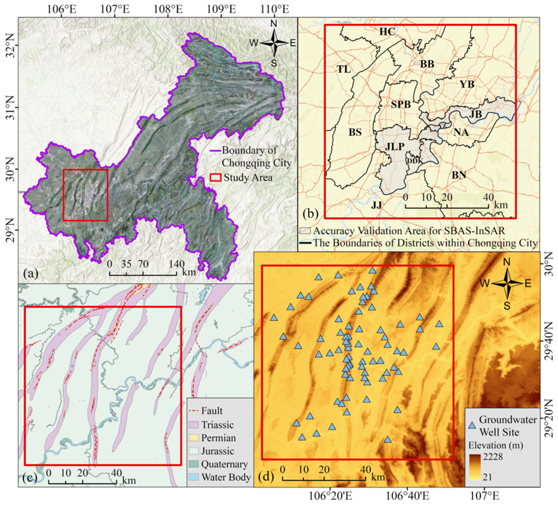
Figure 1. Study area overview map: (a) geographical location of the study area within Chongqing, (b) administrative district distribution across the study area (TL: Tongliang District; HC: Hechuan District; BB: Beibei District; BS: Bishan District; JJ: Jiangjin District; JLP: Jiulongpo District; SPB: Shapingba District; DDK: Dadukou District; BN: Ba’nan District; NA: Nan’an District; JB: Jiangbei District; YB: Yubei District), (c) geologic ages of the strata and fault distribution, and (d) topography and location of groundwater well sites.
Remotesensing 17 03539 g001
Figure 2. The overall workflow of the study.
Remotesensing 17 03539 g002
Figure 3. Land classification maps from 2018 to 2024 derived using the random forest classifier, which achieved good overall accuracy and kappa index.
Remotesensing 17 03539 g003
Figure 4. The scores of the feature importance.
Remotesensing 17 03539 g004
Figure 5. The land cover classification results with a local zoom obtained by random forest classifier-coupled null importance feature selection method.
Remotesensing 17 03539 g005
Figure 6. Cumulative land deformation and velocity maps of the study area: (a) time series distribution of cumulative land deformation from 2018 to 2024, and (b) spatial distribution of land deformation velocity from 2018 to 2024.
Remotesensing 17 03539 g006
Figure 7. Land subsidence velocity maps of the study area: (a) spatial distribution of land subsidence velocity from 2018 to 2024, and (b) cumulative land subsidence time series at points P1–P4, labeled in areas of significant land subsidence.
Remotesensing 17 03539 g007
Figure 8. The impervious surface extraction results in the study area from 2018 to 2024.
Remotesensing 17 03539 g008
Figure 9. Time series of urbanization intensity index and land subsidence velocity from 2018 to 2024.
Remotesensing 17 03539 g009
Figure 10. The land deformation along the Chongqing metro lines in the study area: (a) spatial distribution of metro lines; (b) Land deformation velocities within the buffer zones along the metro lines. Red rectangles highlight four significant subsidence zones adjacent to the metro line segments I, J, K, and L; (c,d) display land deformation velocities measured at monitoring points within 600 m on either side of metro line segments I and J, respectively; (e,f) show cumulative land deformation along monitoring profiles HH’ and GG’, respectively.
Remotesensing 17 03539 g010
Figure 11. Comparison of land subsidence between the newly opened lines and existing lines: (a) time series curve of land deformation five metro lines opened before 2020, and (b) increase in land subsidence within three months after operation for the newly opened metro lines.
Remotesensing 17 03539 g011
Figure 12. Time series of groundwater depth, cumulative land deformation, temperature, and precipitation from 2021 to 2024: (a) spatial distribution of groundwater depth from 2021 to 2024, (b) time series of cumulative land deformation and groundwater depth from 2021 to 2024, and (c) average summer temperature and precipitation from 2021 to 2024.
Remotesensing 17 03539 g012
Figure 13. Spatial distribution of anthropogenic factors from 2018 to 2023 (PD: population density; RND: road network density; NTL: nighttime light).
Remotesensing 17 03539 g013
Figure 14. Spatial distribution of climate factors from 2018 to 2023 (TEMP: temperature; PRE: precipitation; RH: relative humidity; WS: wind speed).
Remotesensing 17 03539 g014
Figure 15. Spatial distribution of land surface factors from 2018 to 2023 (LST: land surface temperature; ENDISI: enhanced normalized difference impervious surface index; WD: water density; EVI: enhanced vegetation index).
Remotesensing 17 03539 g015
Figure 16. Spatial distribution of topographic and geological-tectonic factors.
Remotesensing 17 03539 g016
Figure 17. The q-values for each driving factor of land subsidence (** represent a highly significant correlation, * represent a significant correlation).
Remotesensing 17 03539 g017
Figure 18. The result of the interaction detection between the driving factors.
Remotesensing 17 03539 g018
Figure 19. Spatial distribution of MGWR regression coefficients for each driving factor: (a) RND: road network density; (b) PRE: precipitation; (c) ELE: elevation; (d) ENDISI: enhanced normalized difference impervious surface index; (e) PD: population density.
Remotesensing 17 03539 g019
Figure 20. Comparison and validation of SBAS-InSAR and PS-InSAR results: (a) land deformation velocity histograms, and (b) correlation coefficient plot of land deformation velocity.
Remotesensing 17 03539 g020
Figure 21. Spatial distribution of cumulative land subsidence in 2024.
Remotesensing 17 03539 g021
Table 1. Information on the Sentinel-1A and Sentinel-2 data.
SatelliteProduct TypeVariablesSpatial Resolution/
Pixel Size
Temporal
Resolution
Acquisition Dates
Sentinel-1Aground range
detected
products
VV polarization, VH polarization20 × 22 m/10 × 10 m12 days25 August 2018, 20 August 2019, 26 August 2020, 9 August 2021; 4 August 2022; 23 August 2023; 29 August 2024
single look complex productsVV polarization2.7 × 22 m–3.5 × 22 m/
2.3 × 14.1 m
12 days9 January 2018 to 27 December 2024
(103 Images)
Sentinel-2Level-2ABand02, Band03, Band04, Band05, Band06, Band07, Band08, Band08a, Band11, Band1210 m (Band02, Band03, Band04, Band08);
20 m (Band05, Band06, Band07, Band08a, Band11, Band12)
5 days27 August 2018; 17 August 2019; 26 August 2020; 1 August 2021; 11 August 2022; 16 August 2023; 25 August 2024
Table 2. Details on the driving factors data.
TypeFactorSourceDescriptionSpatial/
Temporal
Resolution
Time
Span
Anthropogenic
factors
Nighttime lights (NTL)https://dataverse.harvard.edu/, accessed on 3 January 2025NTL data were derived from the global NPP-VIIRS-like nighttime light dataset with a spatial resolution of 500 m. It clearly reflects the intensity and temporal changes in nighttime lights [44,45].500 m/
yearly
2018–2023
Population density (PD)https://landscan.ornl.gov/, accessed on 12 January 2025Population data are from LandScan, developed by Oak Ridge National Laboratory [46]. PD is calculated by dividing the total population by land area and reflects how people are distributed in space [47].1000 m/
yearly
2018–2023
Road network density (RND)https://www.openstreetmap.org/, accessed on 12 January 2025Road data comes from OpenStreetMap, an open-source mapping community. RND is computed as the road length divided by the regional area. It reflects the scale and capacity of the urban road network [48,49].1000 m/
yearly
2018–2023
Topographic and
geological-tectonic
factors
Elevation
(ELE)
https://earthdata.nasa.gov/, accessed on 13 January 2025ELE comes from the Digital Elevation Model data of the Shuttle Radar Topography Mission conducted by the National Aeronautics and Space Administration in 2000. Based on this, slope and aspect data were generated. They describe the terrain features of the study area [50,51].30 m2015
Aspect
Slope
Distance to faults (DF)https://www.ngac.cn/
, accessed on 18 January 2025
Geological map data come from the National Geological Archives of China. Faults and stratum information were extracted. Stratum refers to geological layers representing different geological periods. The stratum data were rasterized, and the Euclidean distance to faults was calculated. These data characterize the fundamental geological conditions of the study area [52,53].1000 m2014
Stratum
Climate factorsTemperature (TEMP)https://data.tpdc.ac.cn/, accessed on 9 January 2025TEMP and PRE data come from the National Tibetan Plateau Data Center. The data were downscaled using the Delta method, integrating the 0.5° global climate dataset from Climatic Research Unit with the high-resolution dataset provided by WorldClim. The dataset has been carefully validated to reliably reflect the spatial and temporal patterns of temperature and precipitation [54,55].1000 m/monthly2018–2023
Precipitation (PRE)
Relative
humidity (RH)
https://cds.climate.copernicus.eu/, accessed on 9 January 2025RH and WS were derived from the ERA5-Land reanalysis dataset provided by the European Center for Medium-Range Weather Forecasts. Monthly mean values were generated by downscaling ERA5-Land data to a 1 km spatial resolution using the Delta method [56]. RH indicates how close the water vapor in the air is to saturation. WS is a direct measure of wind strength.0.25°/
hourly
2018–2023
Wind speed (WS)
Land surfaces
characteristic
factors
Land surface temperature (LST)https://earthdata.nasa.gov/, accessed on 6 January 2025LST comes from the MOD11A2 product by the United States Geological Survey [57,58]. LST reflects the temperature variation in the land surface.1000 m/
8 days
2018–2023
Impervious surface (IS)https://browser.dataspace.copernicus.eu/, accessed on 6 January 2025IS quantifies the proportion of built-up land area modified by human activities. It was acquired by the Enhanced Normalized Difference Impervious Surface Index (ENDISI) was calculated using [59,60]:
ENDISI   = 2   ×   B 2   +   B 12 2 B 4   +   B 8   +   B 11 3 2   ×   B 2   +   B 12 2   +   B 4   +   B 8   +   B 11 3
where B2, B4, B8, B11, and B12 denote the blue, red, near-infrared, shortwave infrared 1, and shortwave infrared 2 bands of Sentinel-2 imagery, respectively.
20 m/
27 August 2018;
17 August 2019;
26 August 2020;
1 August 2021;
11 August 2022;
16 August 2023;
25 August 2024
2018–2023
Water density (WD)https://www.openstreetmap.org/, accessed on 18 January 2025Waterbody data come from OpenStreetMap [61], an open source mapping community. WD is calculated by dividing the total length of water bodies by the area of each region. It reflects the distribution of water bodies in the area.1000 m/
yearly
2018–2023
Enhanced
vegetation
index (EVI)
https://search.earthdata.nasa.gov/, accessed on 9 January 2025EVI is extracted from the MOD13A3 product [62,63]. It is used for analyzing vegetation greenness over time and space on a global scale.1000 m/
monthly
2018–2023
Table 3. Summary of the feature extraction data in this study.
DatasetVariables
Original
bands
S1-VV polarization, S1-VH polarization,
S2-Band02, S2-Band03, S2-Band04, S2-Band05,
S2-Band06, S2-Band07, S2-Band08, S2-Band08a,
S2-Band11, S2-Band12
Synthetic Aperture
Radar (SAR) and
spectral
indices
features
Dual Polarization SAR Vegetation Index (DPSVI)
Normalized Difference Vegetation Index (NDVI)
Normalized Difference Vegetation Index red-edge 1 (NDVIre1)
Soil Adjusted Vegetation Index (SAVI)
Modified Normalized Difference Water Index (MNDWI)
Bare Soil Index (BSI)
The Normalized Difference Built-up Index (NDBI)
Texture
features
Mean-VV, Mean-VH, Variance-VV, Variance-VH, Homogeneity-VV, Homogeneity-VH, Contrast-VV, Contrast-VH, Dissimilarity-VV, Dissimilarity-VH, Entropy-VV, Entropy-VH, Angular Second Moment-VV, Angular Second Moment-VH, Correlation-VV, Correlation-VH
Table 4. Classification samples in this study. Please see the Supplementary Materials for further information.
Land Cover
Type
Training DataValidation DataClassification Criteria
Forest land1201514Forest, shrub, etc.
Farmland798342Cropland: planted and unplanted.
Water863370Lakes, rivers, reservoirs, etc.
Urban land1632700Urban buildings, concrete roads, etc.
Bare land931399Sites under construction, etc.
Grassland827354Natural, artificial, and other grassland.
Table 5. Classification of interaction types between two driving factors.
Interaction RelationshipType of Interaction
q ( X f     X g )     >     Max ( q ( X f   ) ,     q ( X g ) ) Two-factor enhancement
q ( X f     X g )     >     q ( X f   ) + q ( X g ) Nonlinear enhancement
q ( X f     X g )   =   q ( X f   ) + q ( X g ) Independent
q ( X f     X g )     <     Min ( q ( X f   ) ,   q ( X g ) ) Nonlinear weakening
Min ( q ( X f   ) ,   q ( X g ) )     <     q ( X f     X g )     <     Max ( q ( X f   ) ,   q ( X g ) ) Single-factor nonlinear weakening
Table 6. The accuracy of Random Forest, Support Vector Machine, Artificial Neural Network, and Maximum Likelihood Classification.
Land Cover TypesRandom ForestSupport Vector
Machine
Artificial Neural
Network
Maximum Likelihood Classification
OA (0.88)  K (0.88)OA (0.86)  K (0.81)OA (0.83)  K (0.80)OA (0.76)  K (0.72)
UAPAKUAPAKUAPAKUAPAK
10.960.970.950.930.940.920.910.920.890.880.890.86
20.900.920.910.860.880.870.830.850.840.800.820.79
31.000.970.970.960.930.930.930.900.900.900.870.87
40.830.790.770.820.730.710.780.690.670.740.650.62
50.730.770.750.680.710.690.640.670.650.600.630.60
60.920.840.820.870.790.770.830.750.730.790.710.69
Note. Land cover types: 1. Forest land, 2. Farmland, 3. Water, 4. Urban land, 5. Bare land, 6. Grassland. Metrics: OA (Overall Accuracy), K (Kappa index), PA (Producer’s Accuracy), UA (User’s Accuracy).
Table 7. Classification performance across datasets and methods, including metrics such as overall accuracy and kappa index.
Feature Extraction DatasetOverall AccuracyKappa Index
Original bands0.880.87
SAR and spectral indices features0.910.89
Texture features0.770.74
Original bands + SAR and spectral indices features0.910.90
SAR and spectral indices features + Texture features0.790.79
Original bands + SAR and spectral indices features + Texture features0.850.83
Feature selection results0.950.94
Table 8. Confusion matrices for impervious surface area and non-impervious surface area.
Land
Cover
Types
2018201920202021202220232024
ISANonISANonISANonISANonISANonISANonISANon
ISA65347655456455564060620806208061090
Non501929481931401939351944301949251954201959
OA = 0.96
Kappa = 0.91
OA = 0.96
Kappa = 0.91
OA = 0.95
Kappa = 0.90
OA = 0.97
Kappa = 0.92
OA = 0.94
Kappa = 0.90
OA = 0.97
Kappa = 0.92
OA = 0.97
Kappa = 0.93
Note. ISA is impervious surface area, and Non is non-ISA; OA (Overall Accuracy); Kappa (kappa index).
Table 9. Severity distribution proportions for land subsidence grading.
Land Subsidence Velocity (mm/yr)Low
0~10
Relatively Low
10~30
High
30~40
Total
Number of monitoring points2,787,493113,7593522,901,644
Percentage96.07%3.92%0.01%100%
Disclaimer/Publisher’s Note: The statements, opinions and data contained in all publications are solely those of the individual author(s) and contributor(s) and not of MDPI and/or the editor(s). MDPI and/or the editor(s) disclaim responsibility for any injury to people or property resulting from any ideas, methods, instructions or products referred to in the content.