Abstract
Displacement back-analysis is a crucial approach to enhance the effectiveness of landslide monitoring data. To improve the computational efficiency and reliability of large-scale three-dimensional landslide displacement inversion, this study develops a novel Landslide Displacement Intelligent Dynamic Inversion Framework (LDIDIF), which integrates the Bayesian displacement back-analysis (BBA) approach, a Long Short-Term Memory (LSTM) surrogate model, and the RANdom SAmple Consensus (RANSAC) algorithm. Specifically, BBA is employed to dynamically calibrate geotechnical parameters with uncertainty, the LSTM model replaces traditional numerical simulations to reduce computational cost, and RANSAC filters inlier observations to enhance the robustness of the inversion model. A case study of the Dawanzi GNSS landslide is conducted. Results show that the LSTM surrogate model achieves prediction errors below 2 mm and enhances computational efficiency by approximately 50,000 times. The RANSAC algorithm effectively identifies and removes GNSS outliers. Notably, LDIDIF significantly reduces the uncertainty of shear strength parameters within the slip zone, yielding a calibrated displacement precision better than 10 mm. The calibrated model reveals that the landslide is buoyancy-driven and that frontal failure may trigger progressive deformation in the rear slope. These findings offer valuable insights for landslide early warning and reservoir operation planning in the Dawanzi area.
1. Introduction
Landslide monitoring and early warning for individual slopes is essential for the precise prevention and mitigation of geological hazards [1,2,3,4]. Numerical simulation remains one of the most powerful tools for analyzing landslide failure mechanisms and evaluating slope stability [5,6,7]. Displacement back-analysis, which calibrates geotechnical parameters using deformation monitoring data to improve simulation precision, has become a core technique in landslide monitoring and early warning systems [8,9,10,11,12]. In this context, displacement back-analysis is regarded as a crucial approach to enhance the effectiveness of landslide monitoring data.
Accurate geotechnical parameters are fundamental to the success of numerical simulations. Although such parameters can be obtained through in situ or laboratory tests, they may not fully capture the true mechanical behavior of rock and soil masses, resulting in discrepancies between simulations and field observations [13,14,15]. Bayesian displacement back-analysis (BBA) addresses this challenge by incorporating monitoring data to update the probability distributions of geotechnical parameters. This approach allows for uncertainty quantification and improves the reliability of simulation-based assessments. Recent studies have demonstrated the effectiveness of sequential Bayesian updating using time-series data, which enhances model precision and predictive capability [16,17]. Moreover, by combining BBA with reliability analysis, researchers have been able to evaluate slope safety factors and failure probabilities directly based on observational data [18,19,20]. The incorporation of subsurface pore pressure and displacement monitoring has also been shown to reduce parameter uncertainty [21,22]. Notably, Dai et al. [23] highlighted the advantages of integrating surface and subsurface data, which can substantially improve the convergence and efficiency of BBA. These findings highlight the critical importance of monitoring data in the displacement back-analysis process.
Currently, multi-source monitoring systems—“air-space-ground-subsurface” platforms—have largely overcome the limitations of single-technique observation. These systems enable comprehensive tracking of landslide evolution at high spatial and temporal resolutions [24,25,26,27,28,29]. For example, technologies such as inclinometers and multipoint extensometers can directly capture deformation along the slip surface and help identify failure precursors in advance. Meanwhile, the integration of GNSS, Interferometric Synthetic Aperture Radar (InSAR), terrestrial laser scanning, Unmanned Aerial Vehicles (UAVs), and robotic total stations enables the acquisition of surface displacement data with high spatial and temporal resolution. However, due to environmental conditions, sensor limitations, and immature automated data processing algorithms, the acquired monitoring data often contain errors [30,31,32], posing significant challenges for displacement back-analysis. As a result, current landslide monitoring data are characterized by multi-source heterogeneity, error contamination, and high spatiotemporal resolution.
To address the multi-objective optimization challenges posed by the integration of diverse monitoring datasets, several strategies have been proposed [33,34,35,36]. Nevertheless, gross errors remain inevitable in automated deformation monitoring [37,38], and robust estimation techniques for displacement back-analysis remain underexplored. Furthermore, displacement back-analysis requires repeated forward simulations, and the frequent updating of model parameters based on high-frequency data can dramatically increase computational demands. This challenge is especially pronounced in large-scale three-dimensional (3D) models, where a single simulation may require several hours or longer. Recently, machine learning-based surrogate models have emerged as efficient alternatives to traditional numerical simulations. They are capable of accelerating computations by three to four orders of magnitude [39,40,41].
In summary, improving the computational efficiency and robustness of displacement back-analysis is crucial to achieving precise monitoring and early warning for individual landslides. Building upon the conventional BBA framework, this study develops a novel Landslide Displacement Intelligent Dynamic Inversion Framework (LDIDIF), which integrates a machine learning surrogate model and a robust RANSAC-based outlier detection algorithm. A comprehensive case study on the Dawanzi GNSS-monitored landslide is presented to demonstrate the application of the proposed framework, encompassing deformation pattern analysis, hydrological surrogate modeling, dynamic inversion of shear strength parameters, and stability assessment under high reservoir water levels.
2. Study Area and Data
2.1. Geological Background of the Dawanzi Landslide
The Baihetan (BHT) hydropower station, located on the lower reaches of the Jinsha River at the border between Sichuan and Yunnan provinces, China, is the world’s second-largest hydropower project after the Three Gorges Dam. The Dawanzi (DWZ) landslide is situated approximately 22.5 km upstream of the BHT dam site, adjacent to the downstream outlet of the DWZ tunnel on the Hubai Highway, bounded by the Tuandigou (TDG) and Xiaojiasha (XJS) gullies. The DWZ tunnel (K8 + 000 to K8 + 965) directly traverses the landslide body. The main contributing factors to the landslide include gravitational forces, weathering and unloading of rock masses, and river incision. The landslide covers an area of approximately 286,000 m2, with a longitudinal length of 800 m, an average width of 358 m, and an estimated volume of 19.82 million m3, corresponding to an average thickness of 69.3 m. Figure 1a presents a UAV image of the DWZ landslide captured in May 2023.
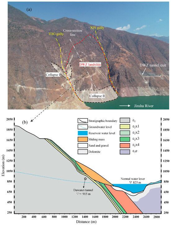
Figure 1.
General information of the study area: (a) UAV image of the DWZ landslide taken in May 2023; (b) typical geological cross-section of the DWZ landslide.
The initial impoundment of the BHT reservoir began on 6 April 2021, with the water level rising from 657.55 m to the normal pool level of 825 m, which was reached on 25 October 2022. Slope failures were observed in several sections of the DWZ landslide both before and after impoundment. Specifically, a collapse occurred in Collapse I prior to impoundment, followed by minor reactivation in the same area and significant failures in Collapse II after the reservoir reached higher water levels.
The crest of the DWZ landslide reaches an elevation of 2250 m. The upper section (2000–2250 m) is gently inclined, with slopes ranging from 15° to 25°. In contrast, the middle section (730–2000 m) exhibits steeper gradients of 30° to 50°, while the landslide toe (below 730 m) is relatively flat, with slope angles less than 15°. The central portion, located between elevations 730 and 850 m, shows the steepest slopes, ranging from 40° to 45°, and the rear scarp slopes range from 30° to 35°.
Figure 1b illustrates a representative geological cross-section of the DWZ landslide. Borehole data and field investigations indicate that the colluvial material is composed predominantly of Quaternary loose deposits (Q). The underlying bedrock comprises medium-thick dolomite of the Lower Cambrian (ε1), thin-bedded sandstone of the Middle Cambrian Xiwangmiao Formation (ε2), and thin- to medium-bedded dolomite of the Upper Cambrian Erdaoshui Formation (ε3e). The bedrock generally strikes north–south and dips 45–55° toward the east. The slip surface mainly consists of weakly cemented gravelly silty clay, which exhibits low shear strength and reduced mechanical stability under saturated conditions, making it highly prone to shear failure. The landslide mass is primarily composed of large angular boulders, with minor amounts of fine-grained soil and coarse gravel. Based on lithological and structural characteristics, the subsurface stratigraphy can be categorized into bedrock (ε1, ε2, ε3), slip zone (SZ group), and landslide mass (LM group).
2.2. Monitoring Data
The first impoundment of the BHT reservoir commenced on 6 April 2021. On 7 July 2021, a large-scale reactivation of the ancient Wangjiashan landslide—approximately 80 km from the dam site—resulted in a complete slope failure. Since then, increasing concern has arisen regarding the stability of reservoir-affected slopes under impoundment conditions. As one of the major potential hazards in the BHT reservoir area, the DWZ landslide has been the focus of intensive deformation monitoring using multiple techniques deployed by relevant agencies.
- (1)
- Environmental monitoring
The environmental monitoring system includes rainfall and reservoir water level observations. Water levels are measured by the reservoir observation station, while rainfall data are collected by rainfall monitoring stations installed at the entrance and exit of the DWZ tunnel. These stations were commissioned on 28 April 2022. Monitoring results indicate that the daily rainfall data from both stations are generally consistent. In this study, rainfall data from the tunnel exit—closer to the landslide mass—are selected for hydrological analysis. Figure 2 presents the time series of reservoir water level and daily rainfall from November 2021 to January 2023.
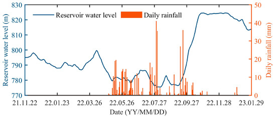
Figure 2.
Reservoir water level variations and daily rainfall near the DWZ landslide.
- (2)
- GNSS monitoring
As shown in Figure 3, the monitoring layout consists of three primary cross-sections and one auxiliary section, encompassing a total of eleven GNSS observation stations. It should be noted that the GNSS1 and GNSS11 stations are situated beyond the boundary of the DWZ landslide and the data from these stations do not represent the displacement of the landslide. Therefore, this study only utilized data from GNSS2-10, excluding the GNSS1 and GNSS11. The automated GNSS monitoring system became operational on 22 November 2021, utilizing the Real-Time Kinematic (RTK) positioning method. Its reference station, installed on the roof of a civil building opposite the slope in a geologically stable area, served as a relatively stable reference point for the monitoring system. Between November 2021 and January 2023, the GNSS stations continuously recorded cumulative displacements in both horizontal (H) and vertical (V) directions. These time-series displacements are depicted in Figure 4.
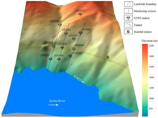
Figure 3.
Layout of monitoring cross-sections and GNSS monitoring stations.
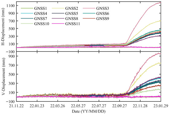
Figure 4.
Cumulative horizontal and vertical displacements recorded by GNSS.
3. Methodology
The proposed LDIDIF framework integrates the BBA approach, a machine learning (ML) surrogate model, and the RANSAC algorithm. Its core objective is to sequentially calibrate uncertain geotechnical parameters using the BBA approach to enable high-precision numerical simulations. Compared to the conventional BBA frameworks, LDIDIF introduces three key improvements: (i) the ML surrogate model replaces traditional numerical simulations to enhance computational efficiency, (ii) the RANSAC algorithm is incorporated to identify and eliminate outlier observations, thereby improving the robustness of displacement inversion, and (iii) uncertain geotechnical parameters are dynamically calibrated based on continuously updated monitoring data. Overall, LDIDIF enables real-time landslide stability assessment with improved precision, reliability, and computational efficiency.
3.1. Overall Architecture
As illustrated in Figure 5, LDIDIF consists of four main modules:
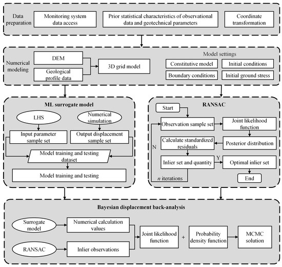
Figure 5.
Overall architecture of the LDIDIF framework.
- (1)
- Data preparation and numerical modeling
This module involves integrating deformation monitoring data with geological investigation results. The prior precision of observational data is estimated based on sensor technical parameters, while the statistical characteristics of geotechnical parameters (e.g., mean, standard deviation, and coefficient of variation) are defined using available prior information. The spatial reference systems of the digital elevation model (DEM) and monitoring datasets are unified to ensure geometric consistency. Subsequently, a 3D mesh model of the landslide is constructed using the DEM and geological cross-sections. Suitable constitutive models, boundary conditions, and initial stress states are applied. These preparatory steps form the basis for displacement back-analysis.
- (2)
- Construction of the ML surrogate model
To reduce the computational burden of repeated forward simulations, ML surrogate models are used to approximate the landslide response. In this study, an LSTM neural network is adopted to construct a hydrologically driven surrogate model. The LSTM architecture is particularly effective for capturing temporal dependencies in time-series data and performs well in scenarios involving small datasets, multiple features, and multi-task learning.
- (3)
- Optimization of observational data using RANSAC
Automated deformation monitoring data are essential for the real-time characterization of landslide deformation patterns. However, such data often contain gross errors due to environmental noise and sensor limitations. To improve the reliability of displacement back-analysis, the RANSAC algorithm is introduced to identify and exclude outliers. By iteratively selecting consistent inlier subsets from large datasets through random sampling and model fitting, RANSAC enhances the quality of observational data used in the Bayesian updating process.
- (4)
- Bayesian dynamic displacement back-analysis
In the LDIDIF framework, geotechnical parameters are treated as random variables with prior probability distributions. A joint likelihood function is constructed based on the surrogate model outputs and inlier observations identified by RANSAC. Bayesian updating is then performed to estimate the posterior distributions of the parameters. Notably, a sequential updating scheme is adopted, wherein the posterior from each update serves as the prior for the next. This iterative structure enables real-time dynamic inversion and supports the development of intelligent, automated landslide early warning systems.
3.2. Bayesian Displacement Back-Analysis
The BBA approach serves as the core of the LDIDIF framework. In this approach, uncertain geotechnical parameters are modeled as random variables, and their probability distributions are iteratively updated using field monitoring data via Bayesian inference. This process effectively reduces parameter uncertainty and improves the reliability of numerical simulations.
Consider a geotechnical system represented as a physical system with a set of uncertain parameters denoted by . Suppose a monitoring station provides displacement observations . The relationship between system response and observations can be represented as follows:
where denotes the numerical simulation model, and represents Gaussian noise with zero mean and standard deviation . Model bias is neglected in this study.
Bayesian updating combines the prior distribution of the parameters with the likelihood of the observed data to produce the posterior distribution:
where, is the likelihood function, which quantifies the consistency between model predictions and observed data. At a specific time t, the likelihood function can be formulated as follows:
In practical applications, multiple monitoring points and heterogeneous data sources are typically available. These observations are commonly assumed to be independent. Accordingly, a separate likelihood function is constructed for each data source, and the joint likelihood is obtained by taking their product.
The prior distribution represents the initial uncertainty of the geotechnical parameters. In this study, is assumed to follow a log-normal distribution, consistent with previous research [42,43]. The probability density function (PDF) of a log-normal distribution is given by the following:
where , , , and denote the mean and standard deviation of the parameter , respectively.
The posterior distribution is typically approximated using the Markov Chain Monte Carlo (MCMC) method. In this study, the Differential Evolution Adaptive Metropolis (DREAM) algorithm is employed due to its high sampling efficiency in high-dimensional parameter spaces. By utilizing a parallel multi-chain strategy, DREAM significantly outperforms traditional algorithms such as Metropolis–Hastings (MH) and Gibbs sampling [44].
3.3. LSTM-Based Surrogate Modeling
The surrogate model is designed to replace conventional numerical simulations in forward computation, that is, to evaluate the function in Equations (1) and (3). In recent years, ML surrogate models have emerged as efficient alternatives to traditional forward modeling in geotechnical applications due to their ability to provide high-speed, sub-millisecond prediction results. Among various ML models—such as Support Vector Regression (SVR), Back Propagation Neural Networks (BPNNs), and eXtreme Gradient Boosting (XGBoost)—LSTM networks have demonstrated superior performance in capturing sequential dependencies and modeling complex nonlinear temporal behaviors [45]. Therefore, LSTM is employed in this study to construct either excavation-driven or hydrologically driven surrogate models for landslide deformation prediction.
In general, the inputs to the LSTM model include geotechnical parameters along with their associated loading conditions (e.g., excavation steps or reservoir water levels), while the output corresponds to the predicted displacement response of the landslide. The training and testing datasets are typically generated using Latin Hypercube Sampling (LHS) in combination with numerical simulations, as described in prior studies [45]. Once the dataset is prepared, the LSTM model is trained through the following steps:
- (1)
- Prepare training samples. Suppose a total of i training samples are available. Each sample consists of m input features and n corresponding target responses . The initial input matrix can be expressed as follows:where represents the n-th input feature value of the i-th training sample.
- (2)
- Normalize the input data. To eliminate differences in scale among input features, normalization techniques such as min–max scaling or Z-score standardization are applied. This results in a dimensionless matrix suitable for model training.
- (3)
- Configure the LSTM network. Key model parameters include the input dimension m, the output dimension n, the number of network layers K, and the number of neurons S per layer. These parameters define the overall structure of the LSTM model.
- (4)
- Train the network. The LSTM model is trained using the back propagation algorithm, which iteratively updates the connection weights between neurons through forward and backward passes to minimize the loss function, typically measured by the mean squared error.
The prediction performance of ML surrogate models is often sensitive to hyperparameter settings. Manual tuning is both time-consuming and inefficient. To address this, optimization algorithms such as Particle Swarm Optimization (PSO) are commonly employed to automatically identify the optimal parameter configurations [46,47].
3.4. RANSAC Algorithm
The RANSAC algorithm is a robust sample selection technique used to identify a high-quality subset of inliers from datasets potentially contaminated with outliers. It operates by performing random sampling and consistency verification to construct optimal models and solutions based on the most representative observations [48,49,50]. In this context, inliers refer to data points that conform well to the model, typically exhibiting residuals within an acceptable threshold, while outliers are observations that significantly deviate from the model due to gross errors, noise, or other anomalies.
In the LDIDIF framework, the RANSAC algorithm is implemented at each time step t to enhance the robustness of BBA. The procedure consists of the following steps:
- (1)
- Random sampling. Randomly select a minimal subset consisting of k observations from the full dataset. This subset is used to generate an initial estimate of the model parameters.
- (2)
- Posterior estimation. Using compute the posterior distribution of the uncertain parameters based on Equation (2). The mean of the posterior distribution is then used to calculate predicted displacements for all monitoring points.
- (3)
- Residual computation and inlier identification. For each observation, compute the residual between the observed displacement and the predicted displacements:Each residual is then compared with a predefined threshold . If , the observation is classified as an inlier. The number of inliers is recorded. Typically, the threshold is set to three times the standard deviation of the observational error.
- (4)
- Iteration and optimal set selection. Repeat steps 1–3 for n iterations. At the end of the process, select the inlier subset that yields the maximum number of inliers. This optimal inlier set is subsequently used to construct the likelihood function for the formal Bayesian updating.
3.5. Data Processing Workflow
A comprehensive case study is conducted using the DWZ landslide as the test site. The data processing workflow includes the following steps:
First, a 3D numerical model of the DWZ landslide is constructed. Based on this model, deformation characteristics and mechanisms are analyzed through a combination of monitoring data analysis and trial numerical simulations.
Second, a LSTM surrogate model driven by the reservoir water level is developed to replace the conventional numerical simulations.
Third, the RANSAC algorithm is applied to the GNSS time-series data to perform consistency checks. Based on the identified inlier observations, the BBA approach is employed to dynamically calibrate the shear strength parameters of the slip zone.
Finally, the calibrated numerical model is used to assess the stability of the DWZ landslide under the highest reservoir water level. This provides scientific support for landslide risk management during high-water-level conditions.
4. Results
4.1. 3D Numerical Modeling
A 3D mesh model of the DWZ landslide was developed using Rhinoceros and Griddle software, based on DEM and representative geological cross-section data (Figure 6). Other software such as FLAC3D 7.0, ANSYS 2022 R1, MIDAS GTS NX 2021, and ABAQUS 2022 can also be used. Practical implementation can refer to the corresponding software manuals. In the model coordinate system, the X-axis aligns with the Jinsha River flow direction (north–south), while the Y-axis follows the landslide movement direction along the riverbank. The model domain measures 2083 m in the X-direction and 3193 m in the Y-direction, with elevations ranging from 0 m to a maximum of 2150 m.
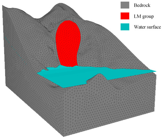
Figure 6.
3D mesh model of the DWZ landslide.
According to geological investigations, the landslide mass is primarily composed of gravelly soil, gravelly silty clay, and bedrock. Consequently, the model was divided into three material zones: the landslide mass (LM group), the slip zone (SZ group), and the underlying bedrock. The geotechnical and hydrological parameters used in this study were obtained from the BHT hydropower station geological survey report and supplemented with bibliographic data [51,52]. Table 1 summarizes the basic numerical model parameters, while Table 2 presents the geotechnical properties of each material group, derived from laboratory tests.

Table 1.
Basic model parameter settings.

Table 2.
Laboratory test values of geotechnical parameters.
Hydromechanical coupling analyses were performed in FLAC3D. The landslide surface was modeled as a free boundary, and fluid flow was governed by Darcy’s law. Under saturated conditions, it was assumed that all pores were fully saturated with water. Fluid-related properties, including water density, porosity, and Biot modulus, are listed in Table 1. The mechanical and hydraulic parameters of each material group are detailed in Table 2.
4.2. Deformation Characteristics and Mechanism
- (1)
- Deformation Characteristics
Reservoir monitoring data (Figure 2) show that the water level remained relatively stable between 775 m and 799 m from November 2021 to September 2022. However, beginning in September 2022, the reservoir water level rose rapidly, reaching the design level of 825 m by 25 October 2022. Rainfall monitoring data indicate that precipitation was concentrated from May to September, with a maximum daily rainfall of 35.5 mm.
GNSS3, located near the landslide toe, recorded the most significant cumulative displacement and is therefore selected as a representative monitoring station. Figure 7 illustrates the cumulative displacement during the rainfall period, while Figure 8 shows the displacement evolution in relation to water level rise. Prior to 12 October 2022, the cumulative horizontal displacement ranged from 48.7 mm to 107.2 mm, corresponding to an average annual displacement rate of 84.6 mm/year. According to the classification criteria [53], the landslide was in a slow-moving stage during this period.
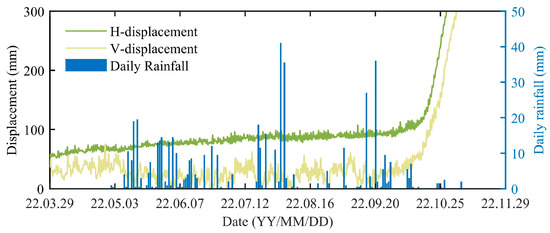
Figure 7.
Cumulative displacement curve of GNSS3 during the concentrated rainfall period.
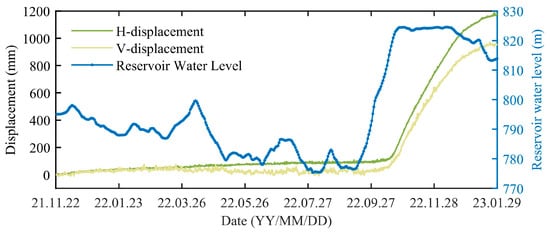
Figure 8.
Relationship between GNSS3 displacement and reservoir water level.
As shown in Figure 7, rainfall from May to September had limited influence on slope deformation. In contrast, Figure 8 reveals a marked acceleration in both horizontal and vertical displacement during the rapid reservoir impoundment period (12 October 2022 to 12 January 2023), indicating a strong correlation between reservoir level rise and slope movement. Specifically, horizontal displacement at GNSS3 increased from 110.1 mm to 1128.3 mm (average 11.1 mm/day), while vertical displacement rose from 52.8 mm to 933.6 mm (average 9.6 mm/day). These results indicate that the landslide was in an accelerating deformation stage during this period
- (2)
- Deformation Mechanism
The DWZ landslide is situated on a steep slope composed primarily of loose gravelly soil and gravelly silty clay. These materials exhibit relatively high permeability (4 × 10⁻⁶ m/s), which promotes both infiltration and drainage. During reservoir impoundment, the high-permeability toe region becomes easily influenced by external water levels, resulting in a rise in groundwater table and increased slope saturation (Figure 9).
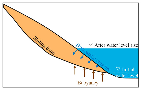
Figure 9.
Conceptual model of the buoyancy-driven landslide mechanism under rising reservoir levels.
To investigate the deformation response under water level rise, the following simulation strategy was employed:
- (1)
- A solid mechanics model was used to compute the initial stress field and achieve geostatic equilibrium under gravity;
- (2)
- A steady-state seepage model simulated pore pressure and effective stress conditions under the low water level (775 m), with all grid displacements reset to zero;
- (3)
- Reservoir levels were then elevated to 785 m, 795 m, 805 m, 815 m, and 825 m, and the resulting displacement fields were computed. Simulation results are shown in Figure 10.
 Figure 10. Simulated surface deformation of the DWZ landslide during water level rise.
The simulations indicate that surface displacement increased significantly with rising water levels, particularly at the landslide toe, where the deformation zone expanded and intensified. This behavior is primarily governed by a buoyancy-driven sliding mechanism:
- The toe region, being highly permeable, responds quickly to reservoir impoundment by raising the internal groundwater level, thereby increasing the buoyant force acting on the landslide mass;
- Submergence also leads to a rise in pore water pressure, which reduces the effective stress and consequently the shear strength along the slip surface;
- These changes collectively lower the normal stress and increase the driving shear stress along the slip surface, leading to failure initiation at the toe and progressive mobilization of the entire landslide mass.
To preliminarily explore the influence of geotechnical parameters on displacement responses, a set of trial simulations was conducted. The results suggest that the cohesion and internal friction angle of the saturated slip zone may significantly affect the deformation pattern. These two parameters are thus treated as uncertain variables in the subsequent back-analysis.
4.3. Hydrologically Driven Surrogate Model
To improve the computational efficiency of displacement back-analysis, a hydrologically driven surrogate model was developed to predict the displacement responses of each GNSS monitoring station under rising reservoir water levels. Beginning on 16 September 2022, the reservoir level increased from 775 m to the design elevation of 825 m and stabilized on 25 October 2022. As shown in Figure 11, the reservoir level rise during this period can be approximated as linear. Taking time in days as the temporal unit, the water level variation can be expressed by the following:
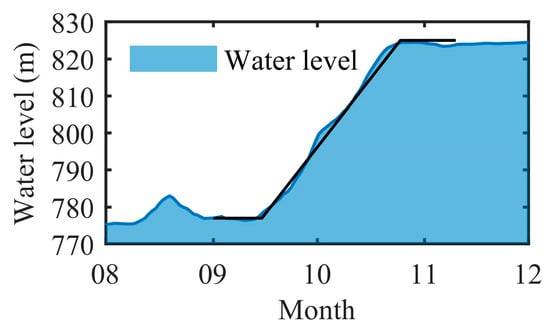
Figure 11.
Linear rise in reservoir water level during the impoundment period.
According to Equation (7), the initial reservoir level is 775 m, with a rise rate of 1.25 m/day. Based on this, 40 water level scenarios were defined. The LSTM surrogate model was then trained to predict displacement responses under these 40 scenarios. The uncertain input parameters were defined as and . A total of 50 parameter samples were generated by LHS, yielding 2000 input combinations when paired with the 40 water levels.
The surrogate model was constructed using an LSTM network. The dataset was randomly split into a training set (80%) and a testing set (20%). The LSTM model achieved a coefficient of determination (R2) of 0.99 on both sets, and the average prediction time per sample was only 3.0 ms—compared to 162 s for traditional numerical simulations—resulting in a ~50,000-fold improvement in computational efficiency. It should be noted that generating the training and testing datasets required approximately 3.75 days. Although dataset generation is time-consuming, once the surrogate model is trained, it can be repeatedly used with extremely low computational cost (3.0 ms per prediction). These results highlight the model’s excellent fitting capability and rapid response. Table 3 summarizes the Root Mean Square Error (RMSE) values of the LSTM predictions across different stations. The testing errors are only marginally higher than those in training, indicating strong generalization and predictive performance.

Table 3.
RMSE of LSTM predictions for training and testing sets (unit: mm).
Figure 12 and Figure 13 illustrate the distribution of prediction errors using violin and box plots. Most prediction errors lie within ±2 mm, with very few outliers. The medians are close to zero, and the narrow interquartile ranges suggest low bias, low dispersion, and high consistency. Despite the large-scale deformation observed at GNSS3—exceeding one meter—the LSTM model maintained excellent predictive performance throughout the impoundment process. Figure 14 compares the LSTM-predicted and FLAC3D-simulated displacements at GNSS3 under varying reservoir levels. The high level of agreement demonstrates the surrogate model’s capability to effectively replicate numerical simulation results and confirms its suitability for hydrologically driven landslide modeling.
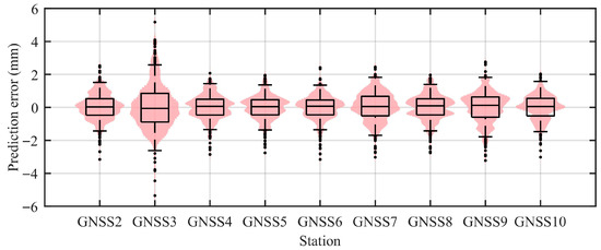
Figure 12.
Violin and box plots of prediction errors for the test set (horizontal direction).
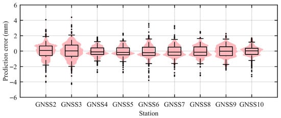
Figure 13.
Violin and box plots of prediction errors for the test set (vertical direction).
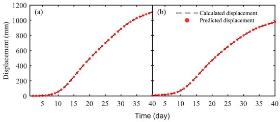
Figure 14.
Predicted vs. FLAC3D-simulated displacement at GNSS3 under different reservoir levels: (a) horizontal direction, (b) vertical direction.
4.4. Dynamic Inversion of Shear Strength Parameters in the Slip Zone
- (1)
- Sample Consistency Check
The consistency check results for the time-series displacement data from nine GNSS stations in both horizontal and vertical directions are shown in Figure 15. In the figure, black markers denote inliers identified by the RANSAC algorithm, while red markers represent outliers corresponding to gross errors. Most outliers are observed in the vertical component, with relatively few in the horizontal direction.
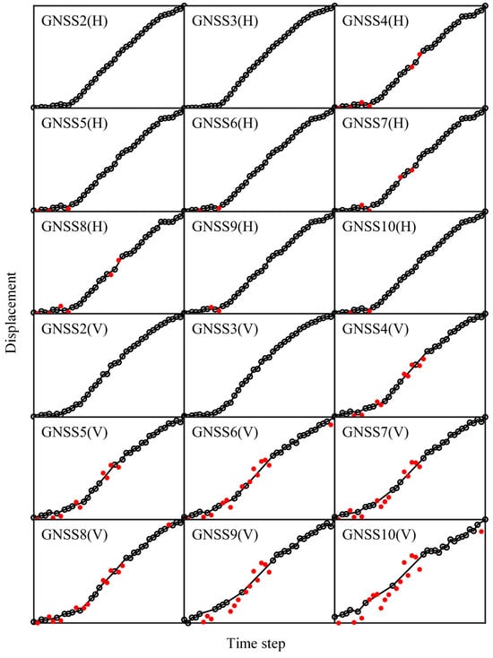
Figure 15.
Consistency check results for time-series displacement at nine GNSS stations.
This finding is consistent with the known limitations of GNSS monitoring, where vertical precision is generally inferior to horizontal precision. Furthermore, the inlier subsets form smooth time series that align with the expected acceleration patterns of landslide deformation, whereas the excluded outliers exhibit sudden deviations or discontinuities.
These results validate the effectiveness of the RANSAC algorithm in extracting high-quality observations that faithfully represent the true deformation behavior of the landslide. This significantly improves the robustness and reliability of the LDIDIF framework.
- (2)
- Inversion Results and Analysis
Based on laboratory testing, prior statistics of uncertain parameters can be obtained, as shown in Table 4. These prior distributions reflect the inherent uncertainty of the geotechnical parameters. The evolution of parameter uncertainty is a key indicator of inversion performance. Figure 16 presents the variation in the coefficient of variation (CV) for the uncertain parameters throughout the Bayesian updating process in LDIDIF. A clear downward trend is observed, indicating a gradual reduction in parameter uncertainty. The CV values converge and stabilize after approximately 28 update steps, which indicates that the obtained posterior parameters are stable and can be reliably used to represent the geotechnical parameters of the slope throughout the update period.

Table 4.
Prior statistics of uncertain parameters.
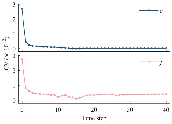
Figure 16.
Evolution of the coefficient of variation for uncertain parameters.
Using the posterior parameters from the 28th update, displacement simulations were performed at nine monitoring stations across 40 time steps. The corresponding RMSE values are shown in Figure 17. Prior to calibration, simulated displacements deviated significantly from the observations, and the prediction errors in both the horizontal and vertical directions almost exceeded 25 mm, with the maximum error reaching over 80 mm (Table 5). After calibration, the simulations matched the observed values closely, with prediction errors in both horizontal and vertical directions remaining below 10 mm. These results confirm that LDIDIF effectively performs dynamic inversion of geotechnical parameters, greatly enhancing the precision of numerical simulations.
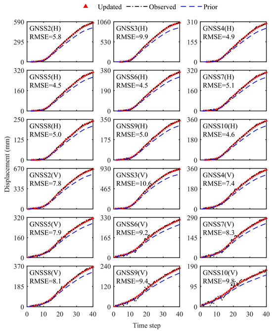
Figure 17.
Comparison of observed vs. simulated displacements before and after parameter calibration.

Table 5.
RMSE of simulated displacements under prior vs. updated parameter (unit: mm).
4.5. Stability Analysis Under the Highest Reservoir Water Level
Based on the LDIDIF-calibrated numerical model, stability analyses were conducted along the most severely deformed cross-section (profile 1–1), which includes GNSS2 and GNSS3. To evaluate the influence of reservoir level, two scenarios were simulated: one corresponding to a moderate water level (795 m) and the other to the design maximum level (825 m). The simulated displacement fields under both conditions are shown in Figure 18.

Figure 18.
Simulated displacement along profile 1–1 under the highest reservoir level.
At the 795 m reservoir level, slope deformation is primarily localized near the toe of the slope, adjacent to the slip surface. The displacement contours are sparse and confined, indicating a relatively stable condition. Although some deformation occurs below the waterline, the unloading effect induced by buoyancy remains limited. The residual shear strength along the slip surface appears sufficient to counteract the mobilized shear stress, thereby preventing large-scale failure or progressive sliding.
In contrast, under the 825 m water level condition, both the magnitude and spatial extent of deformation increase significantly. Pronounced displacement is observed at the submerged slope toe, accompanied by denser contour lines and an upslope expansion of the deformation zone along the slip surface. These results suggest that the elevated water level intensifies the buoyancy effect, which in turn reduces the effective normal stress and shear resistance at the slope toe, triggering initial failure in this region. Subsequently, the destabilization at the toe generates a traction effect on the mid and rear sections of the landslide body, leading to amplified deformation throughout the slope.
In summary, the stability of reservoir-induced landslides exhibits strong sensitivity to variations in water level. Under high water conditions, the submerged slope toe is most vulnerable to failure due to buoyancy-induced unloading. Localized failure at the toe can propagate upslope through traction-induced deformation, ultimately threatening the integrity of the entire slope. These findings underscore the critical importance of continuous deformation monitoring at the slope toe during reservoir impoundment and offer scientific guidance for the development of targeted risk mitigation strategies.
5. Conclusions
To improve the computational efficiency and reliability of landslide displacement inversion, this study proposes an intelligent dynamic inversion framework (LDIDIF) that integrates the BBA approach, a ML surrogate model, and the RANSAC algorithm. The proposed framework was validated through a comprehensive case study of the DWZ landslide. Key findings are summarized as follows:
- The LSTM surrogate model achieved an R2 of 0.99 and improved computational efficiency by approximately 50,000 times, enabling rapid and accurate displacement prediction.
- Integration of the RANSAC algorithm effectively identified and excluded gross errors in GNSS observations, significantly enhanced the robustness of the inversion model.
- The proposed framework enabled dynamic and high-precision inversion of shear strength parameters, with calibrated simulations closely matching field measurements within a 10 mm margin.
- Stability analysis revealed that rapid reservoir impoundment substantially reduces the anti-sliding resistance at the slope toe due to buoyancy effects, emphasizing the critical need for continuous deformation monitoring under high-water-level conditions.
Overall, the LDIDIF framework provides a robust and efficient solution for real-time landslide displacement inversion and stability assessment. It demonstrates strong potential for enhancing early warning systems and informing the development of more effective risk mitigation strategies for hydrologically induced landslides.
Author Contributions
Methodology, Y.D. and W.D.; software, Y.D., C.C. and M.A.; investigation, Y.D. and W.D.; writing—original draft preparation, Y.D., J.L. and Q.H.; writing—review and editing, W.D. and Y.D.; visualization, C.C. and J.L.; supervision, W.D.; project administration, W.D.; funding acquisition, W.D., M.A. and Y.D. All authors have read and agreed to the published version of the manuscript.
Funding
This research was supported by the National Natural Science Foundation of China (No. 42174053), the Department of Natural Resources of Hunan Province (No. HNGTCH-2023-05), and Hunan Provincial Innovation Foundation for Postgraduate (No. CX20230099).
Data Availability Statement
The data presented in this study are available on request from the corresponding author.
Acknowledgments
We gratefully thank the editor and anonymous reviewers for their constructive comments, which greatly improved the quality of this manuscript. The authors also extend their sincere appreciation to China Three Gorges Corporation and Sinohydro Engineering Bureau 8 Co., Ltd. for providing the landslide case data and technical support that were essential to this study.
Conflicts of Interest
The authors declare no conflicts of interest.
Abbreviations
| Notation | |
| uncertain parameter (geotechnical parameter) | |
| observed displacement | |
| model response; predicted displacement | |
| Gaussian noise | |
| time state | |
| probability density function | |
| likelihood function | |
| standard deviation of corresponding measurement | |
| mean of logarithm parameter | |
| standard deviation of logarithm parameter | |
| mean of parameter | |
| standard deviation of parameter | |
| number of samples | |
| number of input features; input dimension of the LSTM | |
| number of target responses; output dimension of the LSTM | |
| input features | |
| target responses | |
| minimal subset | |
| number of sample observations | |
| posterior distribution using to compute | |
| residual between the observed displacement and the predicted displacement | |
| predefined threshold | |
| number of inliers | |
| inlier subset | |
| elastic modulus | |
| cohesion | |
| internal friction angle | |
| saturated permeability coefficient | |
| coefficient of determination | |
| Abbreviations | |
| LDIDIF | Landslide Displacement Intelligent Dynamic Inversion Framework |
| BBA | Bayesian displacement Back-Analysis |
| LSTM | Long Short-Term Memory |
| RANSAC | RANdom SAmple Consensus |
| GNSS | Global Navigation Satellite System |
| InSAR | Interferometric Synthetic Aperture Radar |
| UAV | Unmanned Aerial Vehicle |
| DEM | Digital Elevation Model |
| MCMC | Markov Chain Monte Carlo |
| MH | Metropolis–Hastings |
| DREAM | Differential Evolution Adaptive Metropolis |
| SVR | Support Vector Regression |
| BPNN | Back Propagation Neural Networks |
| XGBoost | eXtreme Gradient Boosting |
| LHS | Latin Hypercube Sampling |
| RMSE | Root Mean Square Error |
| CV | Coefficient of Variation |
| BHT | Baihetan |
| TDG | Tuandigou |
| XJS | Xiaojiasha |
| DWZ | Dawanzi |
| LM | Landslide Mass |
| SZ | Slip Zone |
| ML | Machine Learning |
References
- Nava, L.; Carraro, E.; Reyes-Carmona, C.; Puliero, S.; Bhuyan, K.; Rosi, A.; Monserrat, O.; Floris, M.; Meena, S.R.; Galve, J.P.; et al. Landslide displacement forecasting using deep learning and monitoring data across selected sites. Landslides 2023, 20, 2111–2129. [Google Scholar] [CrossRef]
- Zhang, Q.; Bai, Z.W.; Huang, G.W.; Kong, J.X.; Du, Y.; Wang, D.; Jing, C.; Xie, W. Innovative landslide disaster monitoring: Unmanned aerial vehicle-deployed GNSS technology. Geomat. Nat. Hazards Risk 2024, 15, 2366374. [Google Scholar] [CrossRef]
- Wang, H.; Zhong, P.; Xiu, D.; Zhong, Y.; Peng, D.; Xu, Q. Monitoring tilting angle of the slope surface to predict loess fall landslide: An on-site evidence from Heifangtai loess fall landslide in Gansu Province, China. Landslides 2022, 19, 719–729. [Google Scholar] [CrossRef]
- Hu, X.; Tan, F.; Tang, H.; Zhang, G.; Su, A.; Xu, C.; Zhang, Y.; Xiong, C. In-situ monitoring platform and preliminary analysis of monitoring data of Majiagou landslide with stabilizing piles. Eng. Geol. 2017, 228, 323–336. [Google Scholar] [CrossRef]
- Ju, L.Y.; Xiao, T.; He, J.; Xu, W.F.; Xiao, S.H.; Zhang, L.M. A simulation-enabled slope digital twin for real-time assessment of rain-induced landslides. Eng. Geol. 2025, 353, 108116. [Google Scholar] [CrossRef]
- Li, G.; Zhang, Y.; Zhang, Y.; Guo, Z.; Liu, Y.; Zhou, X.; Guo, Z.; Guo, W.; Wan, L.; Duan, L.; et al. Landslide Hazard Prediction Based on UAV Remote Sensing and Discrete Element Model Simulation-Case from the Zhuangguoyu Landslide in Northern China. Remote Sens. 2024, 16, 3887. [Google Scholar] [CrossRef]
- Wang, H.; Tian, G.; Zhao, Y.; Xie, Y.; Zhang, Q.; Xu, A.; Li, X. Dynamic modeling of Meiping landslide process. Nat. Hazards 2019, 96, 879–892. [Google Scholar] [CrossRef]
- Yang, H.Q.; Zhang, L.L. Bayesian back analysis of unsaturated hydraulic parameters for rainfall-induced slope failure: A review. Earth-Sci. Rev. 2024, 251, 104714. [Google Scholar] [CrossRef]
- Li, D.Q.; Zang, H.H.; Tang, X.S.; Rong, G. Efficient Bayesian updating for deformation prediction of high rock slopes induced by excavation with monitoring data. Eng. Geol. 2024, 342, 107772. [Google Scholar] [CrossRef]
- Liu, Q.; Lei, Y.; Yin, X.; Lei, J.; Pan, Y.; Sun, L. Development and application of a novel probabilistic back-analysis framework for geotechnical parameters in shield tunneling based on the surrogate model and Bayesian theory. Acta Geotech. 2023, 18, 4899–4921. [Google Scholar] [CrossRef]
- Dong, K.; Yang, D.; Chen, J.; Zhou, J.; Li, J.; Lu, X.; Pei, L.; Kou, Q. Monitoring-data mechanism-driven dynamic evaluation method for slope safety. Comput. Geotech. 2022, 148, 104850. [Google Scholar] [CrossRef]
- Dai, Y.; Dai, W.; Yu, W.; Bai, D. Determination of Landslide Displacement Warning Thresholds by Applying DBA-LSTM and Numerical Simulation Algorithms. Appl. Sci. 2022, 12, 6690. [Google Scholar] [CrossRef]
- Robson, E.; Milledge, D.; Utili, S.; Dattola, G. A Computationally Efficient Method to Determine the Probability of Rainfall-Triggered Cut Slope Failure Accounting for Upslope Hydrological Conditions. Rock Mech. Rock Eng. 2024, 57, 2421–2443. [Google Scholar] [CrossRef]
- Marzouk, I.; Brinkgreve, R.; Lengkeek, A.; Tschuchnigg, F. APD: An automated parameter determination system based on in-situ tests. Comput. Geotech. 2024, 176, 106799. [Google Scholar] [CrossRef]
- Hu, Y.; Lu, Y. A novel framework for calibrating DEM parameters: A case study of sand and soil-rock mixture. Comput. Geotech. 2024, 174, 106619. [Google Scholar] [CrossRef]
- Li, X.; Huang, F.; Yang, Z. Multisource monitoring data-driven slope stability prediction using ensemble learning techniques. Comput. Geotech. 2024, 169, 106255. [Google Scholar] [CrossRef]
- Sun, Y.; Huang, J.; Jin, W.; Sloan, S.W.; Jiang, Q. Bayesian updating for progressive excavation of high rock slopes using multi-type monitoring data. Eng. Geol. 2019, 252, 1–13. [Google Scholar] [CrossRef]
- Liu, X.; Wang, Y.; Koo, R.C.H.; Kwan, J.S.H. Development of a slope digital twin for predicting temporal variation of rainfall-induced slope instability using past slope performance records and monitoring data. Eng. Geol. 2022, 308, 106825. [Google Scholar] [CrossRef]
- Jiang, S.H.; Papaioannou, I.; Straub, D. Bayesian updating of slope reliability in spatially variable soils with in-situ measurements. Eng. Geol. 2018, 239, 310–320. [Google Scholar] [CrossRef]
- Li, X.Y.; Zhang, L.M.; Jiang, S.H.; Li, D.Q.; Zhou, C.B. Assessment of Slope Stability in the Monitoring Parameter Space. J. Geotech. Geoenviron. Eng. 2016, 142, 04016029. [Google Scholar] [CrossRef]
- Zhang, L.; Wu, F.; Zheng, Y.; Chen, L.; Zhang, J.; Li, X. Probabilistic calibration of a coupled hydro-mechanical slope stability model with integration of multiple observations. Georisk 2018, 12, 169–182. [Google Scholar] [CrossRef]
- Zheng, Y.; Zhang, L.; Zhang, J.; Zheng, J.; Yu, Y. Multi-objective probabilistic inverse analysis of rainfall-induced landslide based on time-varied data. Rock Soil Mech. 2017, 38, 3371–3377+3384. [Google Scholar] [CrossRef]
- Dai, W.; Dai, Y.; Xie, J.; Shen, S.; Shen, G.; Wang, Y. Enhancing Bayesian probabilistic back-analysis efficiency using multi-type surface and subsurface monitoring data: Case study of the Baihetan left bank slope. Comput. Geotech. 2025, 182, 107174. [Google Scholar] [CrossRef]
- Xu, Q.; Zhao, B.; Dai, K.; Dong, X.; Li, W.; Zhu, X.; Yang, Y.; Xiao, X.; Wang, X.; Huang, J.; et al. Remote sensing for landslide investigations: A progress report from China. Eng. Geol. 2023, 321, 107156. [Google Scholar] [CrossRef]
- Zhang, L.; Zhang, R.; Dou, J.; Hou, S.; Xiang, Z.; Wang, H.; Yang, P.; Liu, X. Advancing reservoir landslide stability assessment via TS-InSAR and airborne LiDAR observations in the Daping landslide group, Three Gorges Reservoir Area, China. Landslides 2025, 22, 169–188. [Google Scholar] [CrossRef]
- Zheng, W.; Hu, J.; Lu, Z.; Hu, X.; Sun, Q.; Liu, J.; Zhu, J.; Li, Z. Enhanced Kinematic Inversion of 3-D Displacements, Geometry, and Hydraulic Properties of a North-South Slow-Moving Landslide in Three Gorges Reservoir. J. Geophys. Res. Solid Earth 2023, 128, e2022JB026232. [Google Scholar] [CrossRef]
- Ye, X.; Zhu, H.; Wang, J.; Zhang, Q.; Bin, S.; Schenato, L.; Pasuto, A. Subsurface Multi-Physical Monitoring of a Reservoir Landslide With the Fiber-Optic Nerve System. Geophys. Res. Lett. 2022, 49, e2022GL098211. [Google Scholar] [CrossRef]
- Ebrahim, K.M.P.; Gomaa, S.; Zayed, T.; Alfalah, G. Recent Phenomenal and Investigational Subsurface Landslide Monitoring Techniques: A Mixed Review. Remote Sens. 2024, 16, 385. [Google Scholar] [CrossRef]
- Deng, L.; Yuan, H.; Chen, J.; Zhang, M.; Su, G.; Zhou, Y.; Chen, Y. Experimental investigation and field application of acoustic emission array for landslide monitoring. Landslides 2024, 21, 71–81. [Google Scholar] [CrossRef]
- Shi, J.B.; Huang, Y.S.; Ouyang, C.H. A GPS relative positioning quality control algorithm considering both code and phase observation errors. J. Geod. 2019, 93, 1419–1433. [Google Scholar] [CrossRef]
- Song, J.; Li, H.; He, X. A High-Precision Distributed Microdisplacement Monitoring System: System Design and Data Processing Algorithms. IEEE Trans. Instrum. Meas. 2022, 71, 1–9. [Google Scholar] [CrossRef]
- Wen, Y.; Dai, W.; Yu, W.; Chen, B.; Pan, L. An enhanced RANSAC-RTK algorithm in GNSS-challenged environments. J. Spat. Sci. 2025, 70, 65–84. [Google Scholar] [CrossRef]
- Peng, M.; Li, X.; Li, D.; Jiang, S.; Zhang, L. Slope safety evaluation by integrating multi-source monitoring information. Struct. Saf. 2014, 49, 65–74. [Google Scholar] [CrossRef]
- Sun, Y.; Jiang, Q.; Yin, T.; Zhou, C. A back-analysis method using an intelligent multi-objective optimization for predicting slope deformation induced by excavation. Eng. Geol. 2018, 239, 214–228. [Google Scholar] [CrossRef]
- Li, Z.B.; Gong, W.P.; Zhang, L.; Wang, L. Multi-objective probabilistic back analysis for selecting the optimal updating strategy based on multi-source observations. Comput. Geotech. 2022, 151, 104959. [Google Scholar] [CrossRef]
- Huang, S.; Huang, J.S.; Kelly, R.; Jones, M.; Kamruzzaman, A.H.M. Predicting settlement of embankments built on PVD-improved soil using Bayesian back analysis and elasto-viscoplastic modelling. Comput. Geotech. 2023, 157, 105323. [Google Scholar] [CrossRef]
- Guo, J.; Ou, J.; Wang, H. Robust estimation for correlated observations: Two local sensitivity-based downweighting strategies. J. Geod. 2010, 84, 243–250. [Google Scholar] [CrossRef]
- Li, X.; Wang, L.; Qu, X.; Zhang, S.; Shu, B.; Xu, H. A GPS multipath mitigation method in coordinate-domain considering the effects of gross errors and missing data. Measurement 2024, 225, 114035. [Google Scholar] [CrossRef]
- Zheng, H.; Mooney, M.; Gutierrez, M. Surrogate model for 3D ground and structural deformations in tunneling by the sequential excavation method. Comput. Geotech. 2023, 154, 105142. [Google Scholar] [CrossRef]
- Liu, X.; Kang, F.; Limongelli, M.P. Multi-zone parametric inverse analysis of super high arch dams using deep learning networks based on measured displacements. Adv. Eng. Inform. 2023, 56, 102002. [Google Scholar] [CrossRef]
- Ding, Q.; Guo, C.; Fan, X.; Liu, X.; Gong, X.; Zhou, W.; Ma, G. Multi-source monitoring data helps revealing and quantifying the excavation-induced deterioration of rock mass. Eng. Geol. 2023, 325, 107281. [Google Scholar] [CrossRef]
- Liu, X.; Liu, Y.D.; Yang, Z.Y.; Li, X.Y. A novel dimension reduction-based metamodel approach for efficient slope reliability analysis considering soil spatial variability. Comput. Geotech. 2024, 172, 106423. [Google Scholar] [CrossRef]
- Wang, Y.; Cao, Z.; Li, D. Bayesian perspective on geotechnical variability and site characterization. Eng. Geol. 2016, 203, 117–125. [Google Scholar] [CrossRef]
- Jiang, S.H.; Wang, L.; Ouyang, S.; Huang, J.S.; Liu, Y. A comparative study of Bayesian inverse analyses of spatially varying soil parameters for slope reliability updating. Georisk 2022, 16, 746–765. [Google Scholar] [CrossRef]
- Dai, Y.; Dai, W.; Xie, J. Slope multi-step excavation displacement prediction surrogate model based on a long short-term memory neural network: For small sample data and multi-feature multi-task learning. Georisk 2025, 19, 158–177. [Google Scholar] [CrossRef]
- Gordan, B.; Armaghani, D.J.; Hajihassani, M.; Monjezi, M. Prediction of seismic slope stability through combination of particle swarm optimization and neural network. Eng. Comput. 2016, 32, 85–97. [Google Scholar] [CrossRef]
- Zhang, P.; Wu, H.-N.; Chen, R.-P.; Chan, T.H.T. Hybrid meta-heuristic and machine learning algorithms for tunneling-induced settlement prediction: A comparative study. Tunn. Undergr. Space Technol. 2020, 99, 103383. [Google Scholar] [CrossRef]
- Chum, O.; Matas, J. Optimal Randomized RANSAC. IEEE Trans. Pattern Anal. Mach. Intell. 2008, 30, 1472–1482. [Google Scholar] [CrossRef]
- Xu, Y.; Boerner, R.; Yao, W.; Hoegner, L.; Stilla, U. Pairwise coarse registration of point clouds in urban scenes using voxel-based 4-planes congruent sets. ISPRS-J. Photogramm. Remote Sens. 2019, 151, 106–123. [Google Scholar] [CrossRef]
- Jiao, Y.; Wang, Y.; Ding, X.; Fu, B.; Huang, S.; Xiong, R. 2-Entity Random Sample Consensus for Robust Visual Localization: Framework, Methods, and Verifications. IEEE Trans. Ind. Electron. 2021, 68, 4519–4528. [Google Scholar] [CrossRef]
- Xing, H.; Zhang, H.; Liu, L.; Yao, D. Comprehensive monitoring of talus slope deformation and displacement back analysis of mechanical parameters based on back-propagation neural network. Landslides 2021, 18, 1889–1907. [Google Scholar] [CrossRef]
- Heidemann, M.; Bressani, L.A.; Flores, J.A. Hydrothermal clays and their influence on slope stability in residual soils of Southern Brazil. Bull. Eng. Geol. Environ. 2021, 80, 795–811. [Google Scholar] [CrossRef]
- Cruden, D.M.; Varnes, D.J. Landslide Types and Processes; Special Report; Transportation Research Board, U.S. National Academy of Sciences: Washington, DC, USA, 1996; Volume 247, pp. 36–75. [Google Scholar]
Disclaimer/Publisher’s Note: The statements, opinions and data contained in all publications are solely those of the individual author(s) and contributor(s) and not of MDPI and/or the editor(s). MDPI and/or the editor(s) disclaim responsibility for any injury to people or property resulting from any ideas, methods, instructions or products referred to in the content. |
© 2025 by the authors. Licensee MDPI, Basel, Switzerland. This article is an open access article distributed under the terms and conditions of the Creative Commons Attribution (CC BY) license (https://creativecommons.org/licenses/by/4.0/).