More Accurate and Reliable Phenology Retrieval in Southwest China: Multi-Method Comparison and Uncertainty Analysis

Highlights

What are the main findings?

• Significant differences exist in the phenological periods derived from different curve-fitting methods, with the CS method being the most suitable for extracting SOS, while the SG method is the most suitable for extracting EOS and POS.
• In the selection of thresholds and SIF datasets, the optimal combination for extracting SOS is the 20% threshold and GOSIF, for extracting EOS, it is the 30% threshold and GOSIF, and the optimal dataset for extracting POS is CSIF.

What is the implication of the main finding?

• Appropriate thresholds, datasets, and curve-fitting methods are crucial for phenological extraction.
• We provide a reference for phenology extraction in regions with frequent cloud cover and widespread evergreen vegetation.

Abstract

Accurate phenological information is crucial for evaluating ecosystem dynamics and the carbon budget. As one of China’s largest terrestrial ecosystem carbon pools, Southwest China plays a significant role in achieving the “dual carbon” goals of carbon peaking and carbon neutrality. However, evergreen forests are widely distributed in this region, and phenology extraction based on vegetation indices has certain limitations, while SIF-based phenology extraction offers a viable alternative. This study first evaluated phenological results derived from three solar-induced chlorophyll fluorescence (SIF) datasets, six curve-fitting methods, and five phenological extraction thresholds at flux sites to determine the optimal threshold and SIF data for phenological indicator extraction. Secondly, uncertainties in phenological indicators obtained from the six fitting methods were quantified at the regional scale. Finally, based on the optimal phenological results, the spatiotemporal variations in phenology in Southwest China were systematically analyzed. Results show: (1) Optimal thresholds are 20% for the start of growing season (SOS) and 30% for the end of growing season (EOS), with GOSIF best for SOS and EOS, and CSIF for the peak of growing season (POS). (2) Cubic Smoothing Spline (CS) has the lowest uncertainty for SOS, while Savitzky–Golay Filter (SG) has the lowest for EOS and POS. (3) Phenology exhibits significant spatial heterogeneity, with SOS and POS generally showing an advancing trend, and EOS and length of growing season (LOS) showing a delaying (extending) trend. This study provides a reference for phenology extraction in regions with frequent cloud cover and widespread evergreen vegetation, supporting effective assessment of regional ecosystem dynamics and carbon balance.

1. Introduction

Vegetation phenology involves the cyclical events of plant development, such as leaf expansion, flowering, fruiting, and leaf fall, serving as critical indicators of vegetation growth and development [1]. Variations in vegetation phenology influence transpiration, photosynthesis, and productivity of vegetation, thereby affecting energy exchange between terrestrial ecosystems and the atmosphere, as well as the ecosystem carbon and water cycles [2,3]. Therefore, accurately monitoring vegetation phenology and analyzing its changing trends are essential for comprehending the dynamic process of ecosystems.

Traditional methods for monitoring vegetation phenology, such as manual recording and ground-based phenological camera observations, have constraints in terms of temporal and spatial resolution [4,5]. Recently, methods employing satellite remote sensing with time-series data have been extensively utilized in regional vegetation phenology research, because of their wide coverage, strong data continuity, and high accuracy [6,7]. However, this method generally necessitates smoothing the raw time-series data to reduce noise, enhance data continuity, and highlight the seasonal variation signal of vegetation [8]. In previous studies, a variety of curve-fitting methods have been employed to smooth time series data, including the Moving Average Window (MA) [9], Savitzky–Golay Filter (SG) [10], Cubic Smoothing Spline (CS) [11], Six-Degree Polynomial Function (PN) [12], Asymmetric Gaussian Function (AG) [13], and Double Logistic Function (DL) [14]. As different curve-fitting methods may result in variations in phenological indicator extraction, evaluating their effectiveness in phenological extraction is essential. Additionally, current vegetation phenology monitoring largely relies on vegetation indices (VIs) derived from reflectance, such as the Normalized Difference Vegetation Index (NDVI) and the Enhanced Vegetation Index (EVI) [6,15]. However, VIs primarily reflect the morphological features of plant canopies and show some inconsistencies with changes in physiological traits, making it difficult to accurately characterize vegetation photosynthetic processes [16,17]. This issue is particularly pronounced in phenological monitoring in tropical and subtropical regions, where evergreen vegetation is widely distributed [14,18]. In recent years, the emergence of solar-induced chlorophyll fluorescence (SIF) has offered a new perspective for phenological extraction. Unlike canopy reflectance products, SIF is a byproduct of the photosynthetic process and is closely connected with it, thus being able to capture changes in vegetation physiology from the initial stage [19]. Therefore, compared with VIs, SIF can track vegetation dynamics more sensitively and in real time from a physiological perspective, demonstrating significant advantages in the phenological extraction of evergreen vegetation [20].

Currently, various SIF products (e.g., GOSIF, CSIF, and RTSIF) have been widely applied in extracting vegetation phenology on scales ranging from regional to global [14,21,22]. However, the spatial resolution of vegetation phenology derived from these SIF datasets is relatively coarse (0.05° × 0.05°). Although relevant studies show that phenology extracted based on flux tower GPP data can serve as ground-measured data to validate SIF-derived phenological [14], the sparse distribution of flux tower sites and their limited observation periods render them insufficiently representative at the regional scale [23], thus failing to fully reflect the true status of vegetation phenology across broader regions. This limitation hinders the accurate evaluation of the dependability of phenological indicators obtained from SIF data using different curve-fitting methods at the regional scale. To address the issue of uncertainty assessment in remote sensing data, the three-cornered hat (TCH) method, as an effective method for quantifying uncertainty, has been extensively applied in the field of remote sensing in recent years [24,25,26]. By analyzing the covariance relationships among various datasets, this method can effectively evaluate the uncertainty of remote sensing data in the absence of ground-truth observations [27]. The TCH method has demonstrated unique advantages in the uncertainty analysis of various remote sensing products, such as land surface temperature [28], soil moisture [29], evapotranspiration [30], and gross primary productivity [31]. However, few studies have focused on using the TCH method to assess the uncertainty of vegetation phenology indicators. Given the importance of SIF data in vegetation phenology monitoring and the scarcity of ground-measured data, this study attempts to apply the TCH method to analyze the uncertainty of phenological indicators derived from SIF data using different curve-fitting methods. The aim is to provide a reliable uncertainty assessment scheme for the extraction of vegetation phenological indicators in regions where ground-measured data are sparse, and to offer a reference for phenological research in related areas.

Southwest China, dominated by a subtropical climate and rich in biological resources, is one of the largest terrestrial carbon pools in China and is critical for maintaining biodiversity and ensuring national ecological security [32]. The region features complex terrains, encompassing plateaus, basins, and mountains. Its unique geographical location, coupled with complex climatic and geomorphological conditions, results in a diverse array of vegetation types and abundant forest resources. Forests constitute approximately 23.6% of the total area of the Southwest China vegetation ecosystem, with evergreen forests particularly widespread, accounting for roughly 48.6% of the total forest area. Therefore, this region is an important and typical area for studying vegetation phenology changes. Recently, the study of vegetation phenology in this region has made some progress. For example, NDVI has been used to extract grassland and forest phenology in western Sichuan [33], EVI has been used to extract forest phenology in Yunnan [15], and leaf area index (LAI) has been employed to extract vegetation phenology in parts of the Yunnan–Guizhou Plateau [34]. However, these studies were primarily based on VIs, which may have introduced considerable uncertainties in the phenology extraction results for this region. On the one hand, Southwest China features high tree species diversity, complex forest stand structures, and widespread distribution of evergreen forests, making it difficult for traditional VIs, due to their own characteristics, to accurately extract their phenological features [14]. On the other hand, Southwest China is often cloudy and rainy, and satellite-based VIs are easily affected by cloud cover and other factors [35]. Compared with traditional VIs, SIF can more effectively reflect the seasonal changes in vegetation phenology from a physiological perspective and is less susceptible to environmental interference factors. Therefore, it is regarded as a reliable remote sensing indicator for monitoring phenology in tropical and subtropical evergreen vegetation regions [36]. In summary, this study employed a variety of SIF datasets and curve-fitting methods to extract the key phenological periods of unchanged land cover pixels in Southwest China from 2001 to 2020, and systematically analyzed the phenological trends across the region and different vegetation types. The primary research contents include: (1) At the site scale, evaluate the extraction performance of six curve-fitting methods on phenological indicators under different thresholds and SIF dataset, to determine the optimal threshold and SIF dataset. (2) At the regional scale, using the optimal threshold and SIF dataset, further evaluate the extraction performance of these six curve-fitting methods on phenological indicators. (3) Based on the optimal phenology extraction results, conduct an in-depth analysis of the spatial patterns and change trends of the start of growing season (SOS), end of growing season (EOS), length of growing season (LOS), and peak of growing season (POS).

2. Materials and Methods

2.1. Study Area

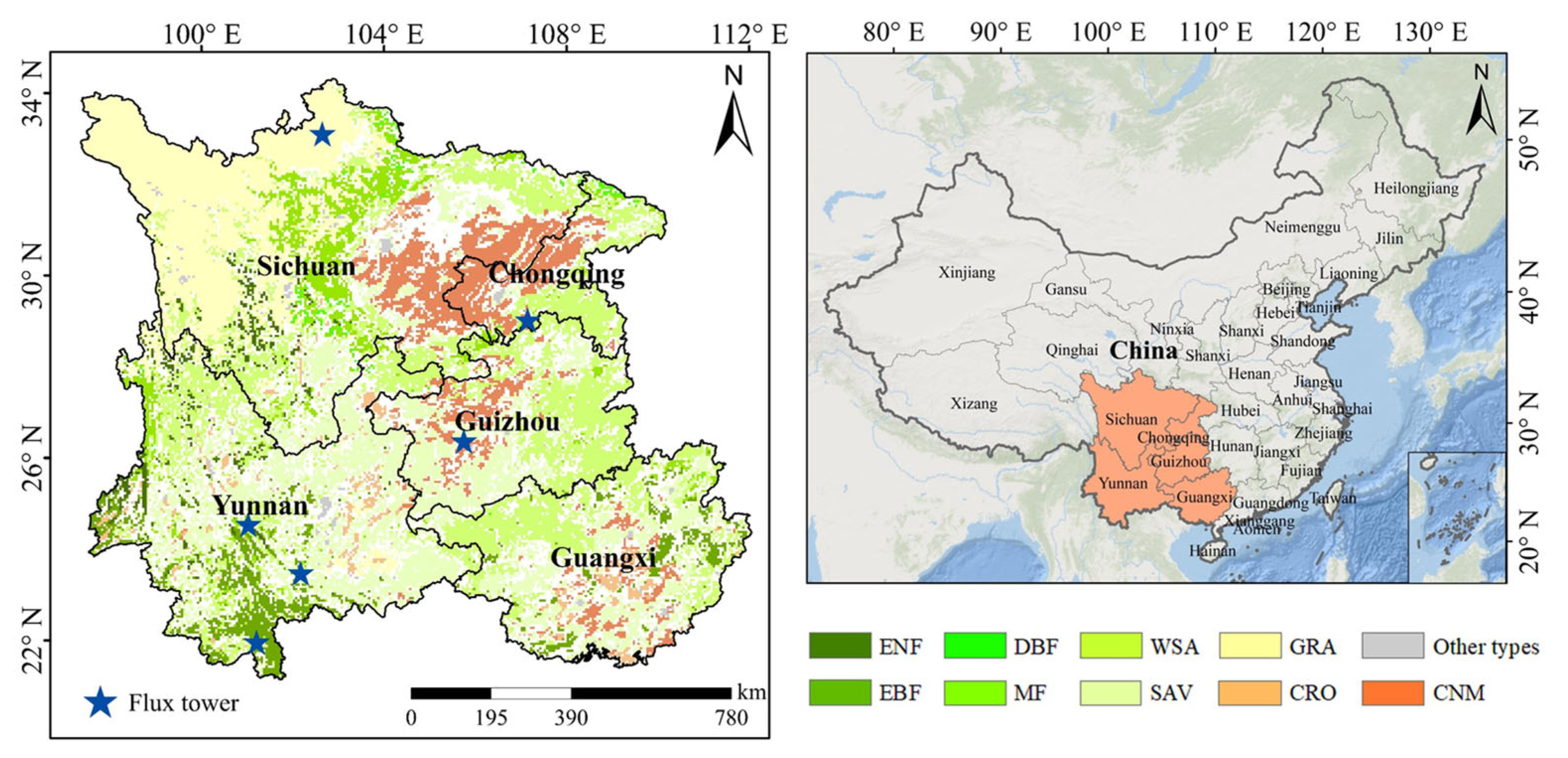
Southwest China, situated in the southwestern part of the country, comprises Yunnan, Guizhou, Sichuan, Guangxi, and Chongqing, with an area of about 137,000 km², accounting for 14.34% of China’s land area. Situated in the mid-low latitudes (20–35°N, 96–113°E), the area is predominantly influenced by a subtropical climate, with abundant precipitation, ample heat, and concurrent rainfall and heat. Additionally, as a typical karst region, its unique geographical location, complex climatic conditions, and topographical features contribute to the region’s rich vegetation resources, making it one of China’s largest terrestrial carbon sinks [37]. The dominant vegetation types include forests, grasslands, and croplands, with evergreen forests being the most widely distributed among forest types. Figure 1 shows the spatial distribution of land cover types and the location of flux sites within the research area.

2.2. Data

2.2.1. GOSIF Data

The first SIF dataset utilized in this research is based on the discrete SIF data from OCO-2, which were aggregated into a 0.05° × 0.05° grid and combined with MODIS remote sensing data and reanalysis meteorological data to generate a global SIF dataset with a spatial resolution of 0.05° (GOSIF) using a data-driven method (http://data.globalecology.unh.edu/ (accessed on 1 May 2025)). The dataset features an 8-day temporal resolution, and it exhibits a strong correlation with flux GPP (R² = 0.73, p < 0.001) [38]. Relative to the original OCO-2 SIF data, GOSIF offers long-term, higher spatial resolution, and global-scale SIF data [38]. It holds significant value for evaluating photosynthetic activities in terrestrial ecosystems and worldwide carbon and water cycles. In this research, we clipped the raster data of Southwest China for the period 2001–2020 from the original GOSIF dataset and removed the negative pixel values.

2.2.2. RTSIF Data

The second SIF dataset utilized in this research is based on the SIF data from TROPOMI, which was aggregated into a 0.05° × 0.05° grid and combined with MODIS reflectance data, surface temperature data, land cover data, PAR data, and vegetation type data to generate a global SIF dataset with a spatial resolution of 0.05° (RTSIF) using machine learning algorithms (https://data.tpdc.ac.cn/zh-hans/data/2b8ffbf4-90ac-4e3d-9ae4-a8be31ae93d4 (accessed on 1 May 2025)). This dataset features an 8-day temporal resolution, and it showed a strong correlation with flux GPP (R² = 0.767) [39]. Relative to the original TROPOMI SIF data and other SIF datasets (GOME-2 SIF and OCO-2 SIF), RTSIF offers long-term, higher spatial resolution, and spatially continuous global-scale SIF data [39]. In this research, we clipped the raster data of Southwest China for the period of 2001–2020 from the original RTSIF dataset and removed the negative pixel values.

2.2.3. CSIF Data

The third SIF dataset used in this study is based on the far-red SIF data from OCO-2, which was aggregated into a 0.05° × 0.05° grid and combined with MODIS visible and near-infrared bands to generate a global SIF dataset with a spatial resolution of 0.05° (CSIF) using machine learning methods (https://data.tpdc.ac.cn/zh-hans/data/d7cccf31-9bb5-4356-88a7-38c5458f052b (accessed on 1 May 2025)). The dataset features a 4-day temporal resolution, characterized by low uncertainty and continuous global coverage, and exhibits a strong correlation with flux GPP [40]. Currently, this dataset has been extensively utilized in vegetation phenology research [41,42,43]. In this research, we clipped the raster data of Southwest China for the period of 2001–2020 from the original CSIF dataset and removed the negative pixel values.

2.2.4. Land Cover Data

This research utilizes the MODIS land cover product (MCD12C1 V61), which is an annual dataset featuring a spatial resolution of 0.05° (https://lpdaac.usgs.gov/products/mcd12c1v061 (accessed on 10 May 2025)). Based on the International Geosphere-Biosphere Programme (IGBP) classification scheme, this dataset provides accurate and robust land cover classification results suitable for characterizing different biome types [44]. In this study, we extracted a total of 20 scenes of land cover type data for Southwest China from 2001 to 2020, and removed the pixels where land cover types changed during these 20 years, retaining only the pixels where land cover types remained unchanged. This processing helps to eliminate the interference of land cover changes on vegetation phenology analysis.

2.2.5. Flux GPP Data

Since vegetation seasonal cycles are well captured by carbon uptake curves, remote sensing observed phenology can be effectively evaluated using carbon flux datasets [45]. This research utilized 29 site-years of GPP data from six flux tower sites in Southwest China, sourced from the National Ecosystem Science Data Center (https://www.nesdc.org.cn/ (accessed on 1 June 2025)). Detailed descriptions of the flux tower sites are presented in

Table 1. Descriptions of the six flux sites utilized in this research.

No.	Station	Lat. (°N)	Lon. (°E)	Vegetation Types	Time Duration
1	ALS	24.53	101.02	Forest	2009–2013
2	YJ	23.47	102.17	Forest	2014–2015
3	JFS	29.02	107.15	Forest	2020
4	PD	26.36	105.75	Forest	2016–2019
5	REG	33.10	102.65	Grassland	2016–2018, 2020
6	XSBN	21.95	101.20	Forest	2003–2015

.

2.3. Method

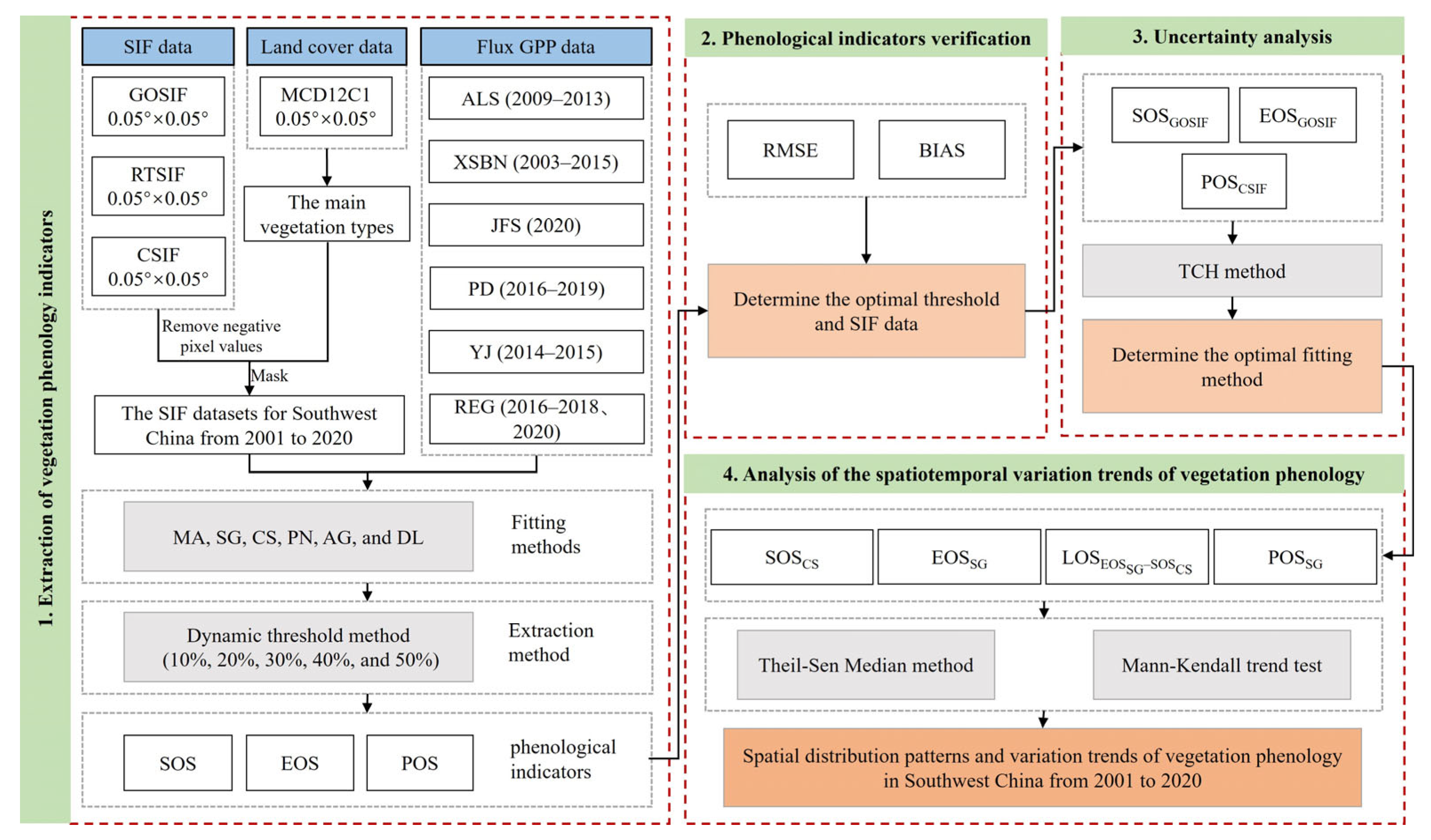
The technical route of this research is depicted in Figure 2, which mainly consists of the following four steps: (1) extraction of vegetation phenology indicators, (2) phenological indicator verification, (3) uncertainty analysis, and (4) analysis of the spatiotemporal variation trends of vegetation phenology.

2.3.1. Phenological Indicator Extraction

When extracting phenological indicators from SIF or GPP, it is essential to fit the original data to remove noise and outliers. This study selected six widely used curve-fitting methods from existing research and categorized them into two types based on the principles of curve fitting: local fitting, including the Moving Average Window (MA), Savitzky–Golay Filter (SG), and Cubic Smoothing Spline (CS); and global fitting, including the Six-Degree Polynomial Function (PN), Asymmetric Gaussian Function (AG), and Double Logistic Function (DL). Detailed information on each curve-fitting method is as follows:

(1)

MA

The method achieves curve fitting through a moving window. Specifically, within a moving window of fixed width, the weight of each point is calculated using a Gaussian density function. The point located at the center of the window has the highest weight, and the weight decreases progressively from the center towards both ends. In this study, we set the moving window width to 15 days based on relevant research [9,46].

(2)

SG

SG is a smoothing method that uses local polynomial least-squares regression within temporal windows. It effectively removes noise while maintaining the original signal’s shape and width and has been extensively employed in vegetation phenological extraction studies [10,47,48]. The formula is as follows:

$${SIF}_i^{\mathrm{*}}={\displaystyle \frac{{\displaystyle {\sum }_{i=-m}^m{C}_{i}SI{F}_{j+i}}}{2m+1}}$$

(1)

where ${SIF}_i^{\mathrm{*}}$ represents the fitted SIF data, m is half of the moving window width, and C_i is the weight corresponding to the value of the i-th point in the moving window. Following relevant studies, we set the window size of the SG filter to 23 days [49].

(3)

CS

CS applies the principle of locally weighted regression to fit the original data by multiple local polynomials. It has been considered a highly flexible curve-fitting method in previous studies [11]. Additionally, the MODIS phenology product (MCD12Q2) has also utilized this fitting method in its calculation and processing. The specific fitting formula is as follows:

$$f_i\left(t\right)={\alpha }_i{\left(t-t_i\right)}^3+{\beta }_i{\left(t-t_i\right)}^2+{\gamma }_i\left(t-t_i\right)+{\delta }_i$$

(2)

where f_i(t) represents the cubic polynomial, t represents the date, and α_i, β_i, γ_i, and δ_i are the coefficients.

(4)

PN

PN is also a widely used curve-fitting method in existing phenological studies. For example, relevant studies have employed sixth-degree polynomial fittings to eliminate noise in the original remote sensing time series data before phenological extraction [12,50]. The formula is as follows:

$$SIF=a+a_{1}t+a_2{t}^2+a_3{t}^3+a_4{t}^4+a_5{t}^5+a_6{t}^6$$

(3)

where t represents the date, and a and a₁ to a₆ are the coefficients of the sixth-degree polynomial.

(5)

AG

AG is also a global fitting method, which is considered capable of capturing complex and subtle variations in curve fitting [51]. The fitting of this method is based on several local functions. Specifically, the local functions formula is as follows:

$$f\left(t\right)=a_1+a_{2}g\left(t;b_1,\dots ,b_5\right)$$

(4)

$$g\left(t;b_{1,}\dots ,b_5\right)=\left\{\begin{array}{l}\mathit{exp}\left[-{\left({\displaystyle \frac{t-b_1}{b_2}}\right)}^{b_3}\right],if t>b_1\\ \mathit{exp}\left[-{\left({\displaystyle \frac{b_1-t}{b_4}}\right)}^{b_5}\right],if t<b_1\end{array}\right.$$

(5)

In the two equations above, Equation (5) is a Gaussian function, where a₁ and a₂ are parameters that determine the baseline and amplitude of the function, respectively; b₁ determines the timing of the extreme value; b₂ and b₃ are related to the width and flatness of the left half of the function; b₄ and b₅ are related to the width and flatness of the right half of the function. The left and right asymmetric Gaussian functions are ultimately integrated through f(t), and the global fitting function formula is as follows:

$$F\left(t\right)=\left\{\begin{array}{l}\alpha \left(\mathrm{t}\right)f_L\left(t\right)+\left[1-\alpha \left(t\right)\right]f_C\left(t\right),t_L<t<t_C\\ \beta \left(\mathrm{t}\right)f_C\left(t\right)+\left[1-\beta \left(t\right)\right]f_R\left(t\right),t_C<t<t_R\end{array}\right.$$

(6)

where α and β are the shear coefficients; f_L, f_C, and f_R correspond to the minimum value on the left, the maximum value in the middle, and the maximum value on the right within the calculation interval, respectively; t_L, t_R, and t_C correspond to the times of f_L, f_C, and f_R, respectively.

(6)

DL

DL is a commonly used global fitting method that performs well in terms of structural flexibility and convergence capability [52], and it has been extensively applied in extracting vegetation phenology [13,14]. The DL fitting formula is as follows:

$$SIF\left(t\right)=a_1+{\displaystyle \frac{a_2}{{\left(1+{\mathrm{e}}^{-d_1\left(t-b_1\right)}\right)}^{c_1}}}-{\displaystyle \frac{a_3}{{\left(1+{\mathrm{e}}^{-d_2\left(t-b_2\right)}\right)}^{c_2}}}$$

(7)

where SIF(t) represents the SIF value on a specific day t within a year, a₁ denotes the value during the winter dormancy period, a₂ denotes the value in the early part of the summer peak period, a₃ denotes the value in the late part of the summer peak period, b₁ and b₂ are the annual median days of spring leaf expansion and autumn senescence turning points, respectively, d₁ and d₂ are the slopes associated with these inflection points, c₁ and c₂ correspond to the dates of the curve’s inflection points.

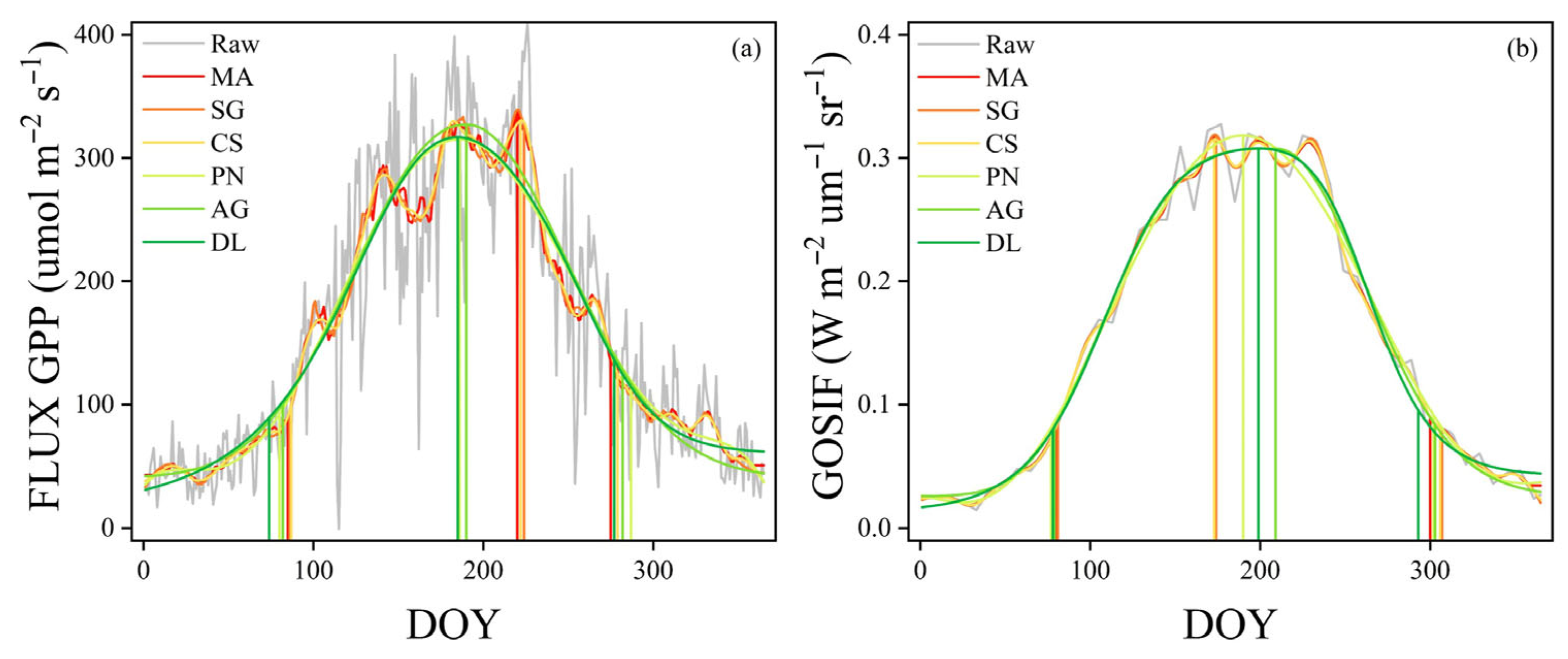
For the fitted time series, the peak date of the fitted curve was defined as the POS [53], while the SOS and EOS were extracted using the dynamic threshold method [15]. Figure 3 shows the fitting effects of different curve-fitting methods and the phenological indicator extraction results. Given that the optimal threshold for extracting phenological indicators of vegetation in Southwest China has not yet been determined, this study selected five different thresholds (including 10%, 20%, 30%, 40%, and 50%) to identify the optimal threshold suitable for SOS and EOS extraction in this region. We first calculated the average root mean square error (RMSE) of SOS and EOS extracted using different thresholds for different SIF datasets under six fitting methods. The threshold that resulted in the lowest average RMSE for SOS and EOS was chosen as the final threshold for this study. The dynamic threshold extraction can be represented by the following equation:

$$SI{F}_{SOS}=0.2\times \left(SI{F}_{max}-SI{F}_{leftmin}\right)+SI{F}_{leftmin}$$

(8)

$$SI{F}_{EOS}=0.3\times \left(SI{F}_{max}-SI{F}_{rightmin}\right)+SI{F}_{rightmin}$$

(9)

where SIF_max represents the maximum value of the SIF time series within a year, SIF_leftmin represents the minimum value before reaching the maximum value, SIF_rightmin represents the minimum value after reaching the maximum value, SOS is the date corresponding to SIF_SOS, EOS is the date corresponding to SIF_EOS, and LOS is the difference between SIF_EOS and SIF_SOS. Additionally, to maintain extraction accuracy, we removed all outliers that exceeded ±3 times the standard deviation from the multi-year average in the phenological extraction algorithm [22].

2.3.2. Accuracy Evaluation

This study utilized the RMSE and bias (BIAS) to evaluate the effectiveness of different thresholds and SIF datasets in extracting vegetation phenology in Southwest China at the site scale. The optimal threshold and SIF dataset for each phenological indicator were selected through comparisons at the site scale and were subsequently used for further processing and analysis.

$$RMSE=\sqrt{{\displaystyle \frac{{\displaystyle \sum _{i=1}^n{\left(a_i-b_i\right)}^2}}{n}}}$$

(10)

$$BIAS={\displaystyle \frac{{\displaystyle \sum _{i=1}^n\left(a_i-b_i\right)}}{n}}$$

(11)

where n represents the number of years, a denotes the phenological indicators extracted from SIF data, b denotes the phenological indicators extracted from flux GPP data, and i indicates the year.

2.3.3. Uncertainty Analysis

Because no phenological verification data at the regional scale corresponds to the SIF scale in Southwest China, assessing the accuracy of extracted phenology regionally is challenging. Based on this, we employed the TCH method to assess the uncertainty of SOS, EOS, and POS extracted by six fitting methods. Unlike conventional error estimation approaches, the TCH method possesses the capability to evaluate uncertainties among three or more datasets without any prior knowledge [54]. Although a reference dataset still needs to be selected in the calculations, studies have shown that the selection of a reference dataset theoretically does not impact the final uncertainty results [28]. Additionally, the method is insensitive to systematic biases and cross-correlated errors in the datasets, and its reliability improves as the number of sequences used in the calculations grows [29]. The main calculation process of TCH is as follows:

We take the uncertainty analysis of the SOS datasets obtained from different fitting methods as an example. For N types of time series, the SOS dataset can be expressed as:

$$SO{S}_i=SO{S}_{true}+{\epsilon }_i, i=1,2,3\dots ,N$$

(12)

where SOS_i represents the i-th SOS dataset, SOS_true represents the unknown true value of the SOS data, ε_i represents the error between the i-th dataset and the true value, N represents the number of SOS datasets, and in this study, N is taken as 6.

Select any one dataset as the reference dataset; the differences between the other datasets and the reference dataset can be expressed as:

$$y_i=SO{S}_i-SO{S}_{ref}={\epsilon }_i-{\epsilon }_{ref}, i=1,2,3,\dots ,N-1$$

(13)

where SOS_ref represents an arbitrary reference SOS dataset, ε_ref represents the time series error between the reference dataset and the true value. Construct an M × (N−1) matrix Y by combining N−1 differential sequences:

$$Y=\left[\begin{array}{cccc}{y}_{11}& y_{12}& \dots & y_{1(N-1)}\\ y_{21}& y_{22}& \dots & y_{2(N-1)}\\ ⋮& ⋮& \ddots & ⋮\\ y_{M1}& \dots & \dots & y_{M(N-1)}\end{array}\right]$$

(14)

where M is the number of time series datasets from each SOS dataset. The phenology extracted in this study is on an annual scale, with a time range of 2001–2020; therefore, M is 20.

The covariance S of the differential sequence matrix Y can be expressed as:

$$S=\mathrm{cov}(Y)=\left[\begin{array}{cccc}{s}_{11}& s_{12}& \dots & s_{1(N-1)}\\ s_{21}& s_{22}& \dots & s_{2(N-1)}\\ ⋮& ⋮& \ddots & ⋮\\ s_{(N-1)1}& s_{(N-1)2}& \dots & s_{(N-1)(N-1)}\end{array}\right]$$

(15)

where s_ij on the diagonal of S (i.e., s_ii) denotes the variance estimates of uncertainty for different SOS datasets, and the rest are covariance valuations. Introduce an N × N covariance matrix R (R is a symmetric matrix). The relationship between R and S can be expressed as:

$$S=J·R·J^T$$

(16)

Here, the matrix J is

$$J_{N-1,N}=\left[\begin{array}{ccccc}1& 0& \dots & 0& -1\\ 0& 1& \dots & 0& -1\\ ⋮& ⋮& \ddots & ⋮& ⋮\\ 0& 0& 0& \dots & -1\end{array}\right]$$

(17)

And the matrix R is

$$R=\left[\begin{array}{cccc}{r}_{11}& r_{12}& \dots & r_{1N}\\ r_{21}& r_{22}& \dots & r_{2N}\\ ⋮& ⋮& \ddots & ⋮\\ r_{1N}& r_{2N}& \dots & r_{NN}\end{array}\right]$$

(18)

where r_ij = r_ji (i, j = 1,2, 3, …, N) is the covariance between the time series ε_i and ε_j, and the diagonal elements r_ij (i = j) are the uncertainty values of each SOS dataset. From Equation (16), we can derive:

$$r_{ij}=s_{ij}-r_{NN}+r_{iN}+r_{jN}$$

(19)

The unknown elements in matrix R can be calculated using Equation (19). More details can be found in the reference [55]. The SOS uncertainty for a single grid can be obtained under the minimum constraint condition.

2.3.4. Trend Analysis

We employed the Theil–Sen median approach to analyze the trend of vegetation phenology in the study area. As a robust non-parametric approach, it is often employed to quantify trends in time series and exhibits strong resistance to outliers [56].

$$\beta =median\left({\displaystyle \frac{x_j-x_i}{j-i}}\right)\left(\forall j>i\right)$$

(20)

where x_i and x_j denote the phenological indicator values for years i and j, β indicates the interannual change trend of the study subject. When β > 0, SOS, EOS, and POS indicate a delay trend, while LOS indicates an extension trend. Conversely, it means that there is a tendency to advance or shorten.

Additionally, we employed the Mann–Kendall (MK) statistical test to analyze the significance levels of phenological trends. As one of the widely used nonparametric tests, the MK test does not assume a particular data distribution and is more robust against outliers [57].

$$Z=\left\{\begin{array}{l}{\displaystyle \frac{S}{\sqrt{Var\left(S\right)}}}\hspace{1em}\left(S>0\right)\\ \hspace{1em}0\hspace{1em}\hspace{1em}\hspace{1em}\left(S=0\right)\\ {\displaystyle \frac{S+1}{\sqrt{Var\left(S\right)}}}\hspace{1em}\left(S<0\right)\end{array}\right.$$

(21)

where $\mathrm{S} = \sum _{\mathrm{i}=1}^{\mathrm{n}-1}\sum _{\mathrm{j} = \mathrm{i}+1 }^{\mathrm{n}}\mathit{sgn} \left({\mathrm{x}}_{\mathrm{j}}-{\mathrm{x}}_{\mathrm{i}}\right)$. When x_j−x_i is less than, equal to, or greater than 0, the corresponding $\mathit{sgn}(x_j-x_i)$ values are −1, 0, and 1, respectively. In addition, Var(S) = n (n−1) (2n+5)/18. When the Z statistics are positive, it denotes an increasing trend; otherwise, it denotes a decreasing trend.

In this study, the confidence level for the MK significance test was set at 95%. The significance of phenological change trends was categorized into the following five classes: significant advance (shortening) (β < 0, p < 0.05), non-significant advance (shortening) (β < 0, p ≥ 0.05), significant delay (extension) (β > 0, p < 0.05), non-significant delay (extension) (β > 0, p ≥ 0.05), and invariably (β = 0).

3. Results

3.1. Effect Evaluation of Different Thresholds and SIF Data Extracts

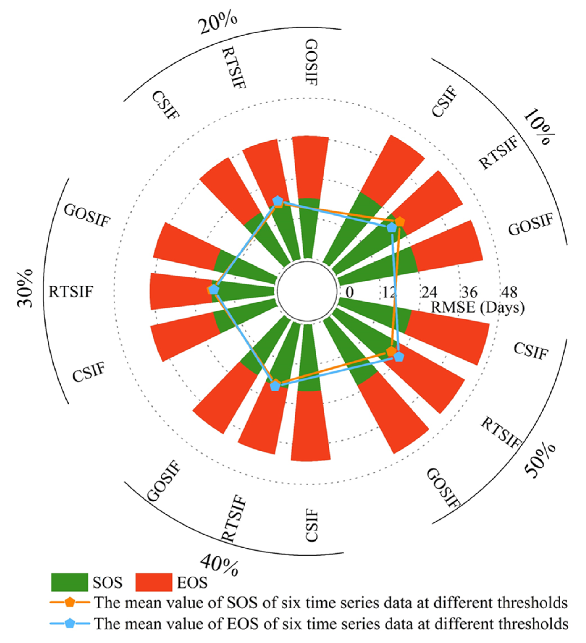
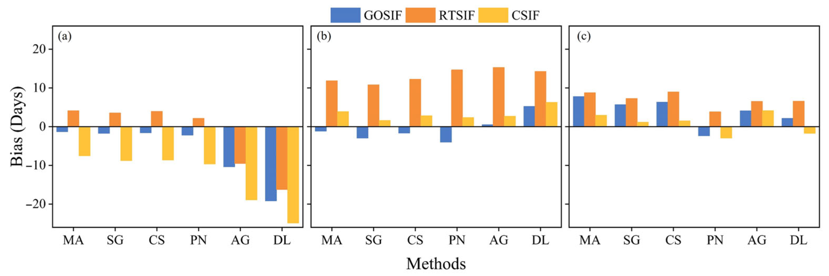
This study first evaluated the effectiveness of different thresholds and SIF data in extracting phenological indicators in Southwest China. The results indicated that for SOS and EOS, the optimal extraction thresholds were 20% and 30%, respectively, and the optimal SIF data were both GOSIF. For POS, the optimal SIF data was CSIF. As shown in Figure 4, when the threshold was set to 20%, the RMSE values for SOS extracted from the three types of SIF data (GOSIF, RTSIF, and CSIF) were 17.9513 days, 17.7799 days, and 17.5133 days, with a mean of 17.7482 days, the lowest among the five thresholds. When the threshold was set to 30%, the RMSE values for EOS extracted from the three types of SIF data were 18.5059 days, 18.4991 days, and 19.2457 days, with a mean of 18.7502 days, also the lowest among the five thresholds. After determining the thresholds, we further compared the differences between the phenological indicators extracted from the three types of SIF data using six curve-fitting methods and those extracted from flux GPP. As shown in Figure 5, for SOS, the bias of the local fitting methods was generally smaller than that of the global fitting methods. Except for RTSIF, SOS extracted from GOSIF and CSIF was earlier than that extracted from flux GPP, and the overall bias of GOSIF was the smallest. For EOS, the bias of the local fitting method was also smaller than that of the global fitting method. Except for GOSIF, EOS extracted from RTSIF and CSIF was later than that extracted from flux GPP, and the overall bias of GOSIF was the smallest. For POS, except for GOSIF and CSIF, the POS extracted from RTSIF was later than that extracted from the flux GPP, and the overall bias of CSIF was the smallest. Based on the above results, this study selected the GOSIF dataset for extracting SOS and EOS, and the CSIF dataset for extracting POS, thereby ensuring the accuracy of phenological indicator extraction.

3.2. Uncertainty Analysis of Phenology Obtained by Different Curve-Fitting Methods

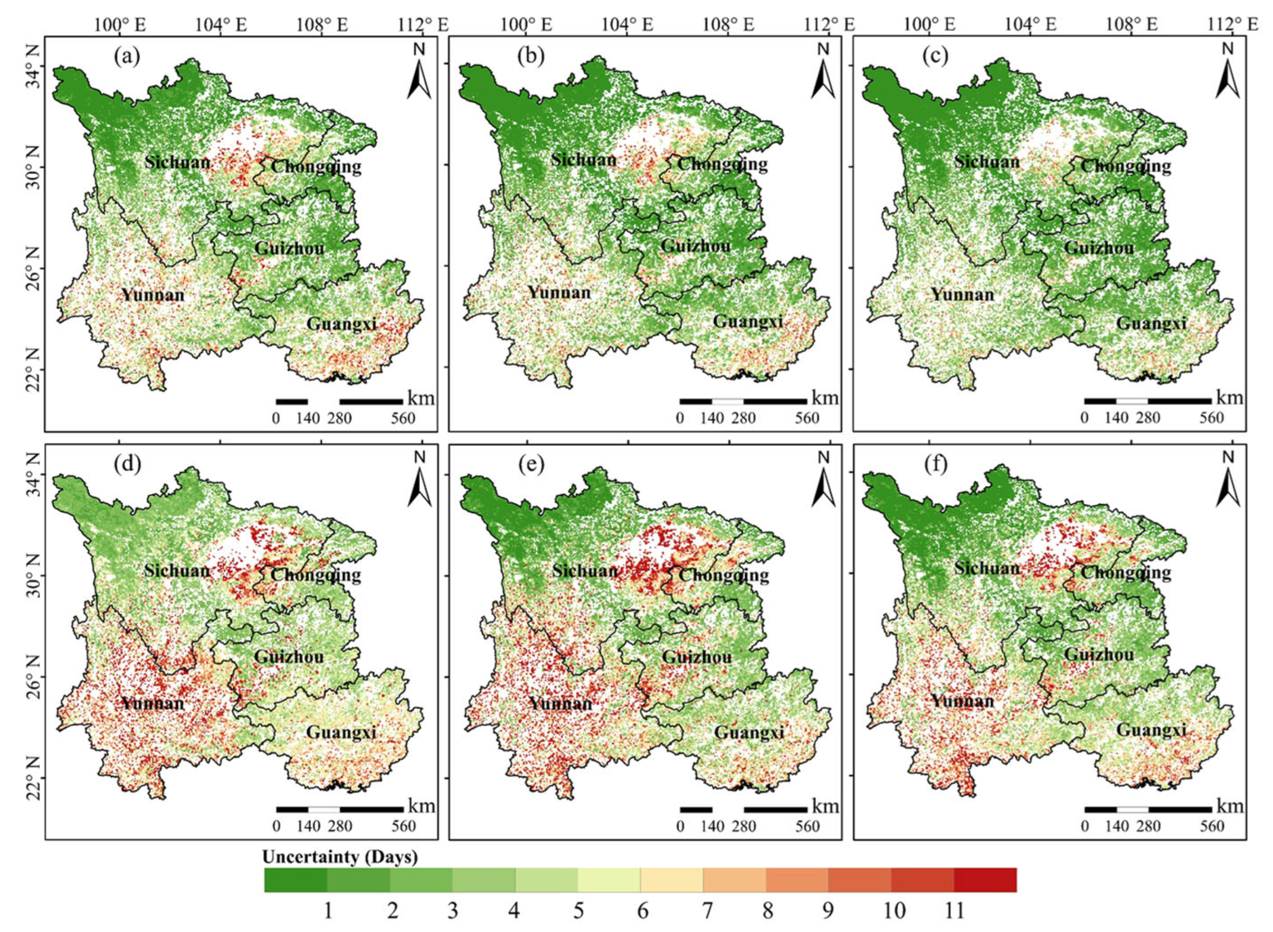
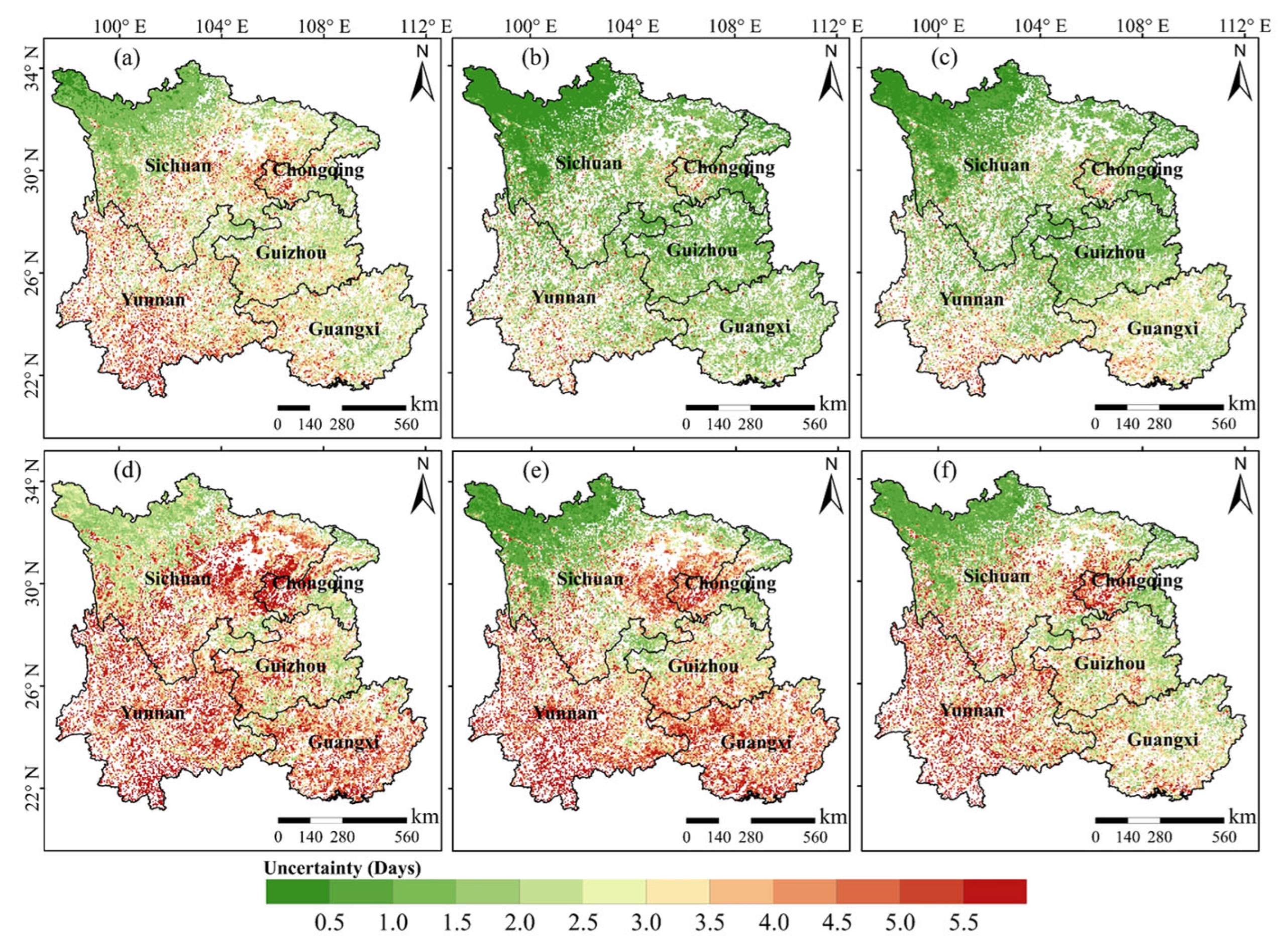
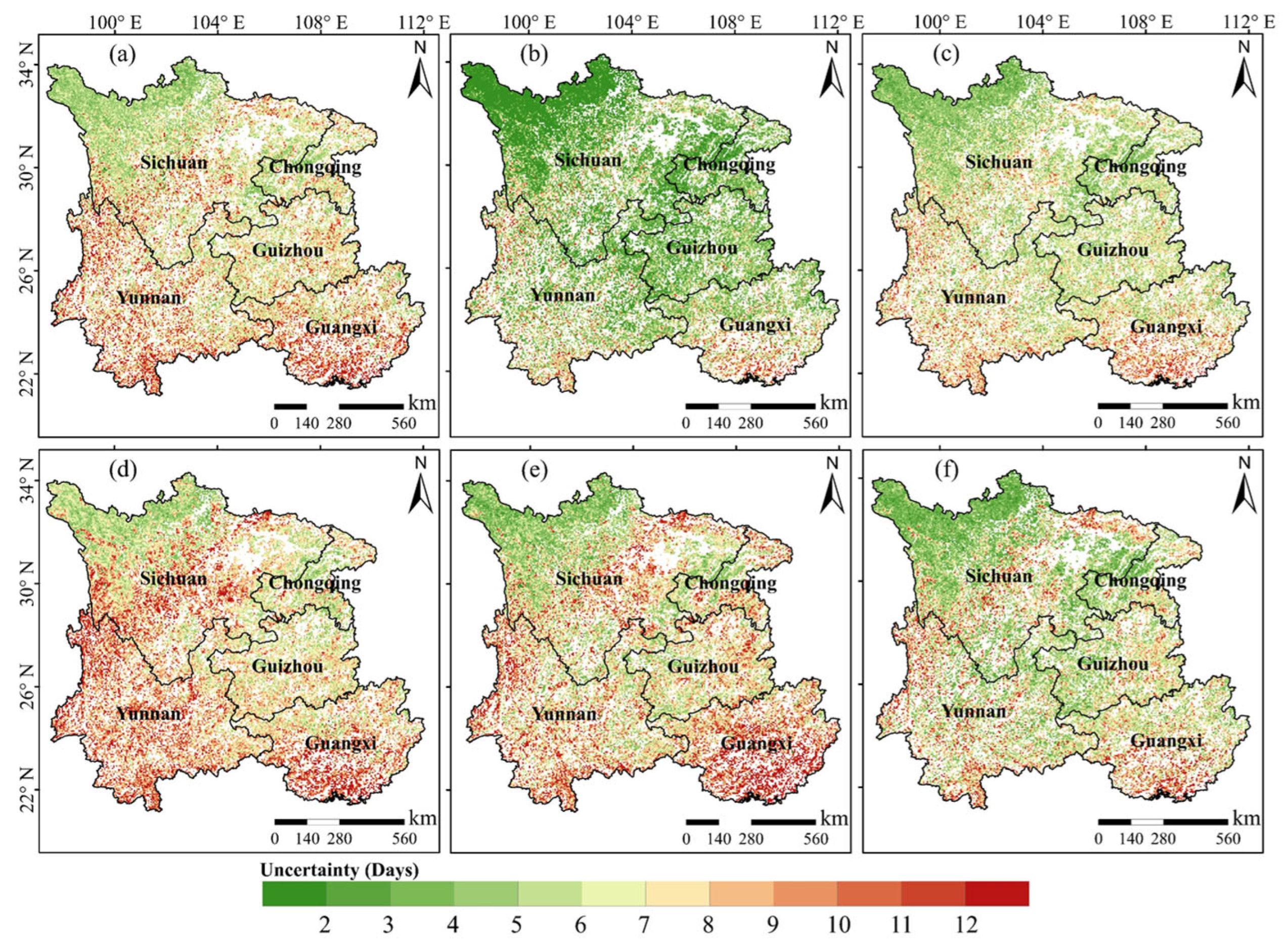
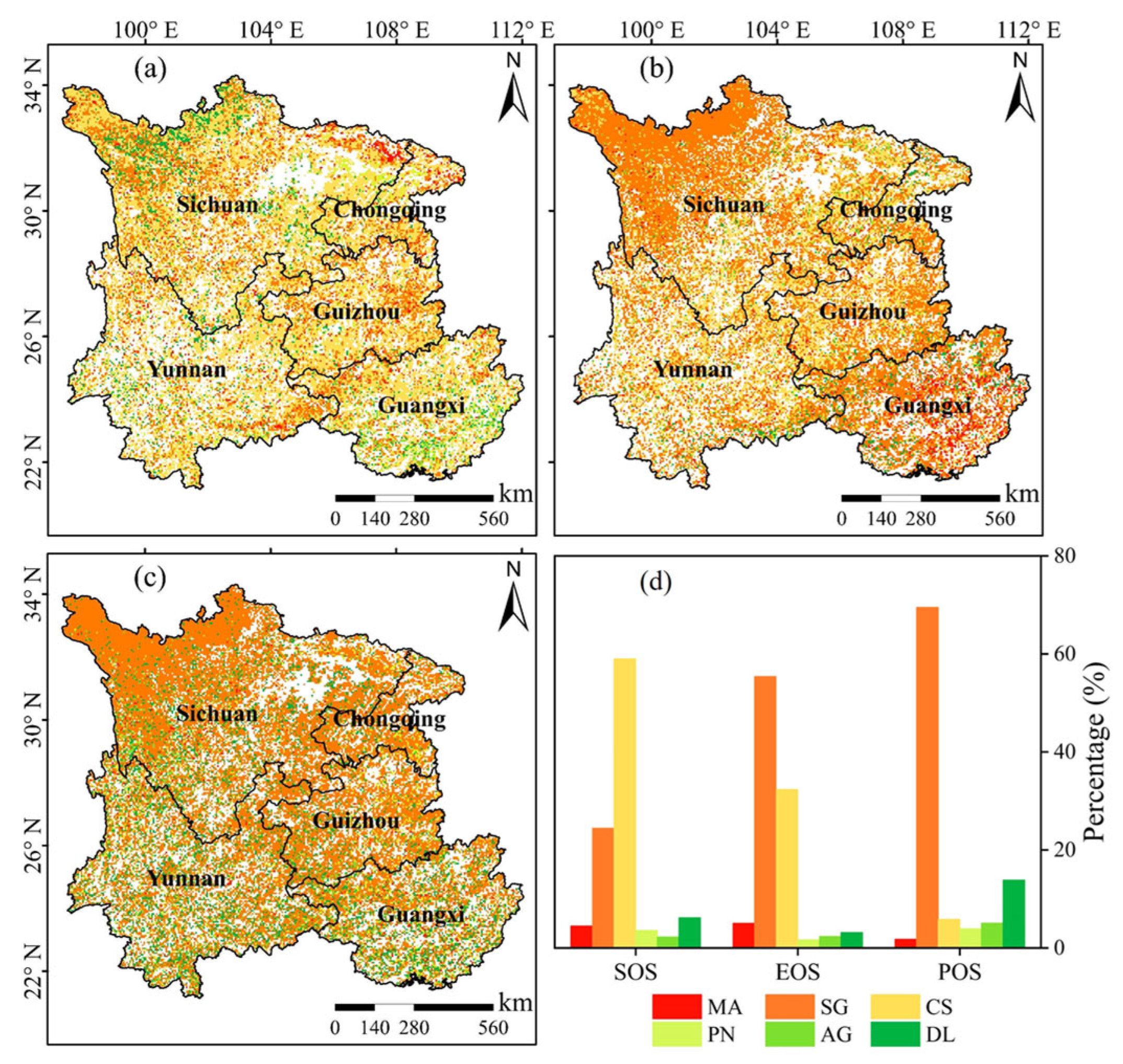
Based on the experimental results from flux sites in Southwest China, we used the optimal threshold and SIF data to extract the phenological indicators based on six curve-fitting methods in Southwest China, and analyzed the uncertainty of the phenological indicators obtained from these six curve-fitting methods using the TCH method. The results showed that among these six fitting methods, the SOS uncertainty obtained from the CS fitting method was the lowest, but the EOS and POS uncertainties obtained from the SG fitting method were the lowest. Firstly, in terms of spatial distribution, the uncertainty in the phenological indicators extracted by the six fitting methods showed certain differences (Figure 6, Figure 7 and Figure 8). Overall, the uncertainty in the phenological indicators obtained from the local fitting methods (MA, SG, and CS) was lower than that from the global fitting methods (PN, AG, and DL). Specifically, regions with higher uncertainty in SOS and EOS were primarily distributed in parts of the Sichuan Basin, Yunnan, Guangxi, and Guizhou (Figure 6 and Figure 7), while areas with higher uncertainty in POS were primarily concentrated in central Sichuan, Yunnan, and Guangxi (Figure 8). Among the six curve-fitting methods, the SOS extracted by the CS method and the EOS and POS extracted by the SG method exhibited the lowest uncertainty. Additionally, based on the uncertainty results, we further analyzed the spatial distribution and proportion of the lowest uncertainty for the six fitting methods (Figure 9). The results indicated that for SOS, the CS method had the lowest uncertainty, accounting for 59.03%, followed by SG (24.46%), DL (6.18%), MA (4.50%), PN (3.59%), and AG (2.24%). For EOS, the SG method had the lowest uncertainty, accounting for 55.39%, followed by CS (32.35%), MA (5.04%), DL (3.17%), AG (2.37%), and PN (1.68%). For POS, the SG method had the lowest uncertainty, accounting for 69.53%, followed by DL (13.86%), CS (5.83%), AG (5.06%), PN (3.93%), and MA (1.79%).

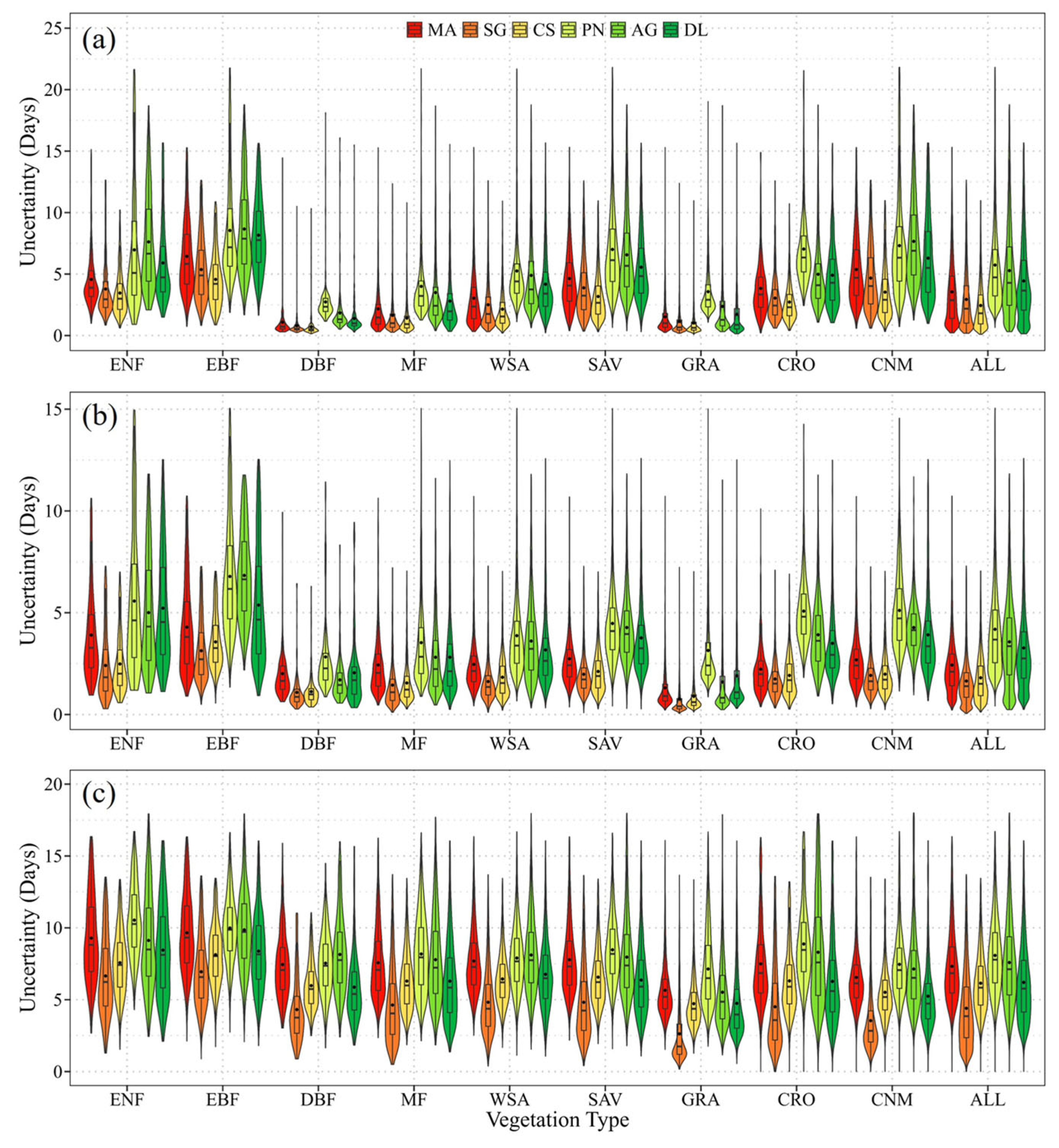
Secondly, in different vegetation types, we found that the uncertainty in their phenological indicators showed significant differences (Figure 10). For SOS, the CS fitting method exhibited the lowest uncertainty across all vegetation types, with a mean of 2.44 days. Specifically, among various vegetation types, the uncertainties for DBF, MF, WSA, and GRA were relatively the lowest, with means of 0.71 days, 1.42 days, 2.15 days, and 1.02 days, respectively, while those for ENF, EBF, SAV, CRO, and CNM were relatively the highest, with means of 3.46 days, 4.57 days, 3.18 days, 2.72 days, and 3.53 days (Figure 10a); for EOS, the SG fitting method had the lowest uncertainty across all vegetation types, with a mean of 1.65 days. The uncertainty distribution characteristics for vegetation types were similar to those for SOS, i.e., the uncertainties for DBF, MF, WSA, and GRA were relatively lower, with means of 1.09 days, 1.45 days, 1.62 days, and 0.75 days, respectively, while those for ENF, EBF, SAV, CRO, and CNM were relatively higher, with means of 2.41 days, 3.13 days, 1.98 days, 2.72 days, and 1.92 days (Figure 10b); for POS, the SG fitting method showed significantly lower uncertainty than other methods across all vegetation types, with a mean of 4.41 days. Overall, ENF and EBF had higher uncertainties, with means of 9.29 days and 6.94 days, respectively, while the uncertainties for the other vegetation types were relatively lower, especially the lowest for GRA, with a mean of 2.63 days (Figure 10c).

3.3. Spatial Distribution Pattern and Change Trend of Vegetation Phenology

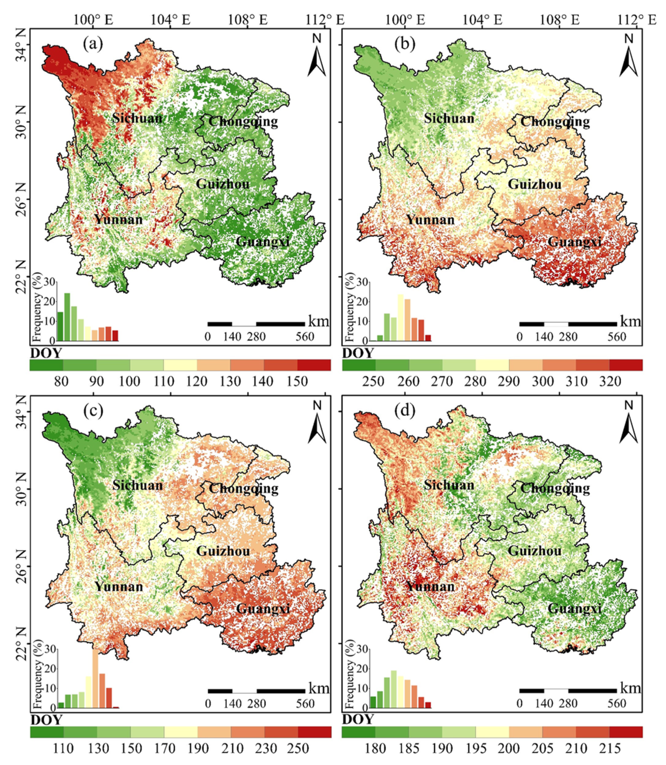
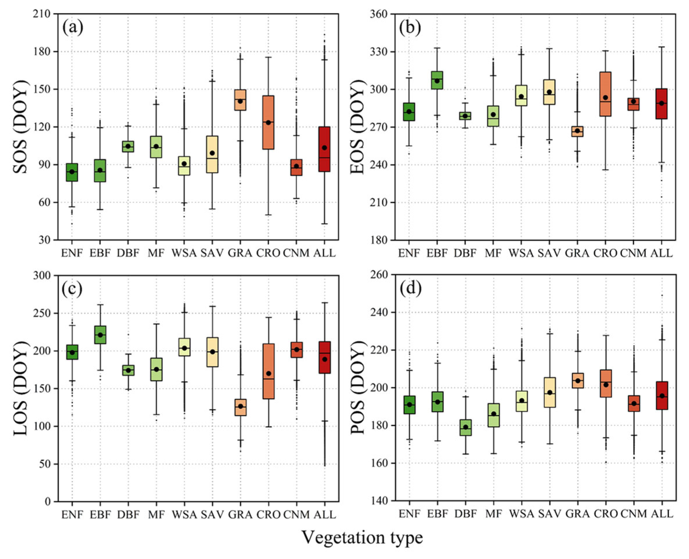
Based on the TCH analysis results, firstly, we adopted the CS fitting method to extract SOS, the SG filtering method to extract EOS and POS, and used the difference between EOS and SOS as LOS. Secondly, we analyzed the spatiotemporal distribution characteristics of the mean values of various phenological indicators in Southwest China from 2001 to 2020. The results showed that the vegetation phenology in this region exhibited obvious spatial heterogeneity in the plateau mountainous areas, northwest and southeast regions, and had transitional characteristics, while the phenological temporal characteristics of different vegetation types also showed certain differences. As shown in Figure 11, the SOS was predominantly concentrated between 80 and 140 days of year (DOY) (72.65%), with earlier SOS mainly occurring in the Sichuan Basin, Chongqing, Guizhou, and Guangxi, while later SOS was primarily distributed in the northwestern part of Sichuan and the eastern part of Yunnan (Figure 11a). The EOS was mainly concentrated between 260 and 320 DOY (93.67%), showing an increasing distribution pattern from northwest to southeast (Figure 11b). The LOS was predominantly concentrated between 110 and 250 days (96.56%), with shorter LOS primarily found in the northwestern part of Sichuan and the northeastern part of Yunnan, while longer LOS was primarily found along the southern border of Yunnan and in Guangxi (Figure 11c). The POS was mainly concentrated between 180 and 215 DOY (91.09%), with earlier POS mainly occurring in Guangxi and later POS mainly in Yunnan and the northwestern part of Sichuan (Figure 11d). As shown in Figure 12, the temporal characteristics of phenology for different vegetation types showed significant differences, among which EBF and GRA had the most concentrated time ranges for SOS, EOS, LOS, and POS, while CRO and SAV had the most dispersed time ranges. Overall, the temporal ranges of EOS and POS were relatively concentrated, while those of SOS and LOS were relatively dispersed.

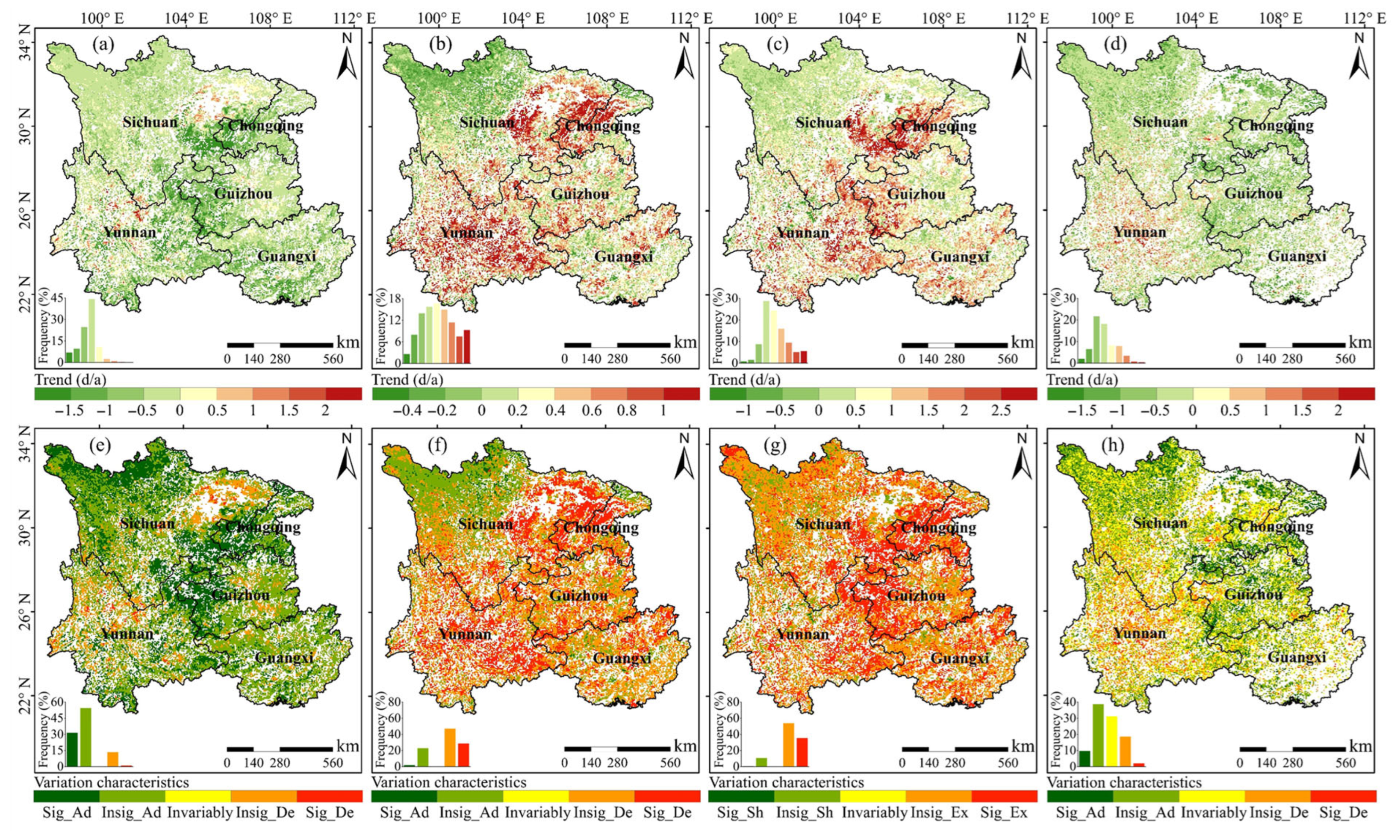
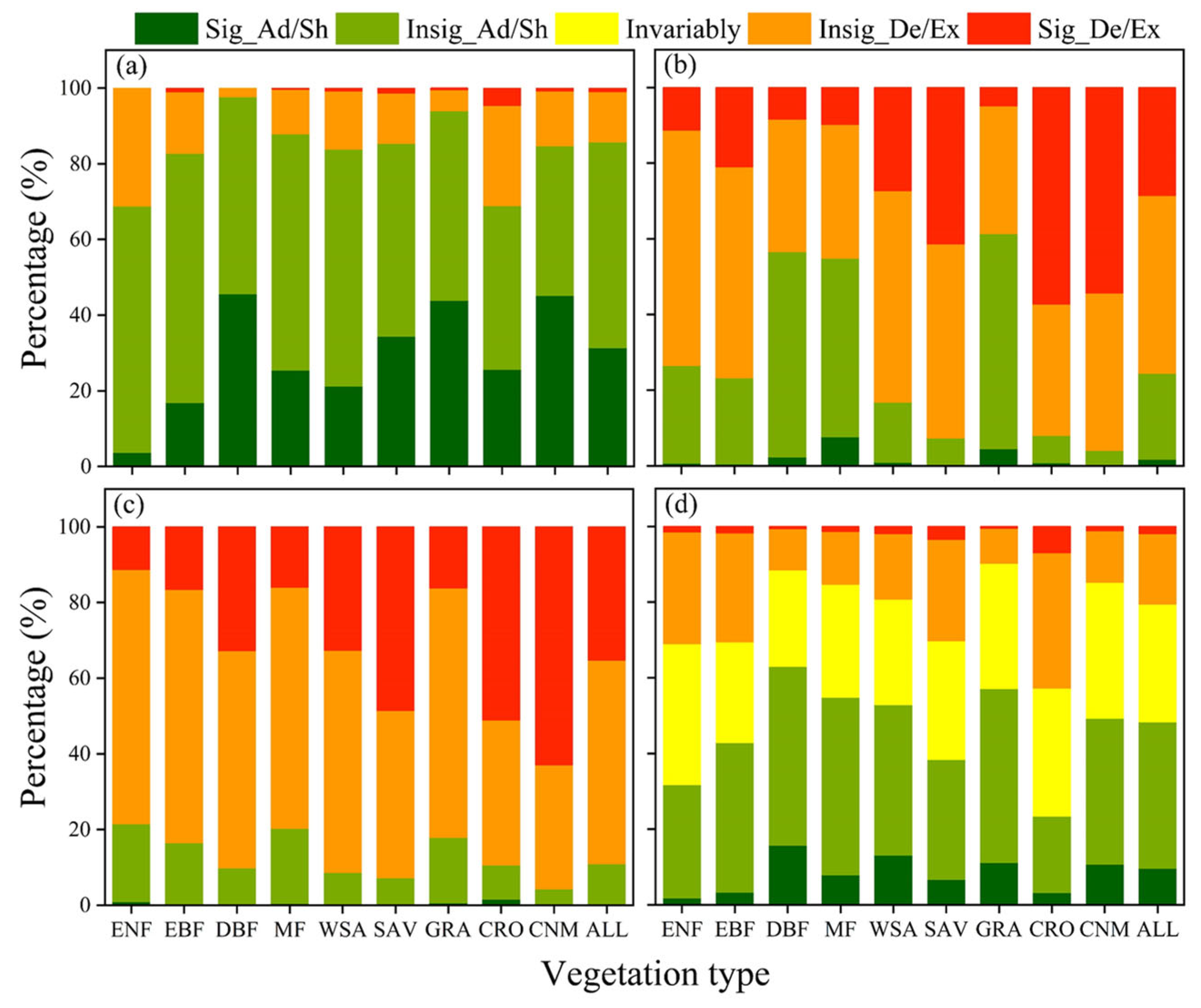
Based on the analysis results of the change trends and significance of vegetation phenology in Southwest China, it was found that SOS and POS in this region overall showed an advancing trend, while EOS and LOS overall showed delaying and extending trends, and there were certain differences among different vegetation types. As shown in Figure 13, for SOS, the majority of the Southwest China showed an advancing trend (85.33%), among which the proportion of advancing 0–0.5 days per year was the highest (44.17%); combined with the significance test results, approximately 54.37% of the study area showed non-significant advancing SOS, mainly concentrated in the northwestern part of Yunnan, eastern Guizhou, and Guangxi. For EOS, the majority of the Southwest China showed a delaying trend (75.52%), among which the proportion of delaying 0–1 days per year was the highest (66.25%); combined with the significance test results, approximately 46.97% of the study area showed no significant delaying EOS, mainly concentrated in Yunnan, Guizhou, Guangxi, and southern Sichuan. For LOS, the Southwest China overall showed a lengthening trend (88.99%), among which the proportion of lengthening 0–1 days was the highest (53.06%); combined with the MK significance test results, approximately 53.72% of the study area showed non-significant lengthening LOS, mainly concentrated in Yunnan, Guangxi, eastern Guizhou, and most regions of Sichuan. For POS, the Southwest China showed a slightly higher proportion of advancing trends (48.36%), among which the proportion of advancing 0–1 days per year was the highest (39.86%); combined with the MK significance test results, approximately 38.67% of the study area showed non-significant advancing POS, mainly distributed in Guizhou, Chongqing, and the northwestern part of Sichuan. Additionally, from the perspective of phenological change trends in different vegetation types, for SOS, all vegetation types were mainly characterized by an advancing trend, among which DBF and GRA had the highest advancing proportions, reaching 97.67% and 93.95%, respectively; For EOS, except for DBF, MF, and GRA, which showed an advancing trend, the other vegetation types exhibited a delaying trend, with the proportion of delay exceeding 73%. For LOS, all vegetation types showed a significant extension trend, particularly DBF, WSA, SAV, and CNM, which exceeded 90%. For POS, except for GRA, all vegetation types exhibited a predominantly advancing trend, with DBF and GRA having the largest proportion of advancement, reaching 63.03% and 57.12%, respectively (Figure 14).

4. Discussion

4.1. Evaluation of Phenological Effects Derived from Different SIF Data and Curve Fitting Methods

To determine the optimal SIF dataset for phenology extraction in Southwest China, this study compared the effects of extracting phenology from different SIF datasets at the site scale. The results show that there are certain differences in extracting vegetation phenological indicators from different SIF datasets. For SOS and EOS, GOSIF is the optimal dataset for their extraction; for POS, CSIF is the optimal dataset for its extraction. Studies on SIF-based phenology extraction also indicate that different SIF datasets exhibit certain differences in extracting vegetation phenology [19]. The reasons for this difference may include the following aspects: Firstly, the temporal resolution. GOSIF and CSIF have different temporal resolutions; GOSIF is 8 days, while CSIF is higher at 4 days. Higher temporal resolution may enable more precise monitoring of vegetation phenology [58], thus potentially leading to CSIF outperforming GOSIF in monitoring the POS. Secondly, the factors considered during data production are different. Compared with CSIF, GOSIF fully considers three types of SIF explanatory variables, namely vegetation, climate, and land cover conditions [38], and may have a stronger seasonality. Therefore, it may have an advantage in extracting phenology in spring and autumn when vegetation growth status changes significantly. In addition to the selection of SIF datasets, curve-fitting methods are also a key factor influencing the reliability of phenology extraction results. In existing phenological extraction studies, whether they are based on SIF data or flux GPP data, the first and inevitable step is to fit the original data to reduce the influence of noise on phenological indicators [59,60]. Studies have indicated that phenological results extracted from different fitting approaches can differ substantially [8]. To assess the applicability of different fitting approaches for phenological extraction in Southwest China, six commonly used curve-fitting methods were selected in this study. Based on their principles, these methods were categorized into two groups: local fitting and global fitting. Based on the phenological indicators obtained by these six curve-fitting methods, we used the TCH method to evaluate their uncertainty. The results show that, regarding spatial distribution, the uncertainty of the phenological indicators derived from the local fitting method is generally lower than that from the global fitting method. This may be because local fitting can better retain the original features of the data [61,62], while global fitting may ignore local details during the fitting process, resulting in deviations between the fitted data and the original data [63], thereby increasing the uncertainty of the phenological indicators. For different phenological indicators, regions with high uncertainty in SOS and EOS are primarily found in the Sichuan Basin, Yunnan, Guangxi, and parts of Guizhou, while regions with high uncertainty in POS are primarily found in Yunnan and Guangxi. The reasons for this phenomenon may include the following: Firstly, the dominant vegetation type in the Sichuan Basin is CNM, which is a mixture of natural vegetation and cropland. The heterogeneity of vegetation types within pixels and multi-seasonal crop planting may generate multi-peak growing season curves, potentially increasing fitting method uncertainties in phenological extraction [64,65]. Secondly, Yunnan, Guangxi, and Guizhou are predominantly karst landform areas, characterized by complex terrain and diverse microclimates. These regions exhibit significant differences in vegetation growth patterns [47], which may lead to error accumulation in different curve-fitting methods and thereby increase the uncertainty of phenological extraction.

In addition, this study further analyzed the minimum uncertainty of phenological indicators extracted using six curve-fitting methods and their uncertainty across different vegetation types. The results show that, for SOS, the CS fitting method has the highest proportion of pixels with the lowest uncertainty; for EOS and POS, the SG filtering method has the highest proportion of pixels with the lowest uncertainty. Among the vegetation types, the uncertainty of SOS extracted by the CS fitting method is the lowest, and the uncertainty of EOS and POS extracted by the SG filtering method is the lowest. This indicates that the CS fitting method is optimal for extracting SOS, whereas the SG filtering method is optimal for extracting EOS and POS in phenological extraction in Southwest China. We speculate that the reasons may include the following: Firstly, the seasonal growth curve of vegetation is usually asymmetric due to differences in physiological changes between spring and autumn [66,67]. In spring, vegetation growth is rapid due to the rapid increase in temperature, resulting in a steep slope of the growth curve [68]. In autumn, vegetation is influenced by factors like photoperiod, temperature, and precipitation, leading to slower leaf senescence and a more gradual decline in the growth curve [69]. This asymmetry may lead to differences in the optimal fitting methods for phenological extraction in spring and autumn. Secondly, the CS method is a piecewise cubic polynomial interpolation fitting method. It is a flexible curve-fitting method [11], which may be more suitable for the spring stage with steeper growing season curves. In contrast, the SG is a filtering method that relies on local polynomial regression. It can effectively remove noise in remote sensing data while retaining the original data features, making it more suitable for the extraction of autumn phenology. This is because vegetation changes in autumn are relatively slow and more susceptible to external factors, which can result in fluctuations in the growing season curve. For POS, the SG filtering method can retain the original data features and identify the peak of the growing season more stably by smoothing out the noise, which may help avoid misjudgments of local fluctuations to a certain extent. In addition, regarding different vegetation types, we observed that for SOS and EOS, ENF and EBF have the highest uncertainty, while DBF and GRA have the lowest uncertainty. For POS, the uncertainty across different vegetation types is generally low, but evergreen forests still exhibit relatively high uncertainty. This phenomenon may be related to changes in vegetation canopy structure [70]. Related studies have shown that SIF is superior to evergreen forests in estimating the phenology of mixed and deciduous forests, which have obvious changes in canopy structure [71]. Given the distinct seasonal variation characteristics of GRA and the uniformity of vegetation type in the region, the uncertainty of phenological indicators based on SIF is relatively low. Additionally, a relevant study has shown that the uncertainty of phenology obtained using the PN fitting method is higher than that of other fitting methods [12]. This is because the curve fitted by PN may deviate more from the original vegetation data, leading to significant differences between the phenological period values of the fitted curve and the original vegetation curve. These discrepancies may further increase the uncertainty in the phenology extracted using PN fitting.

4.2. Analysis of Spatial and Temporal Variation in Vegetation Phenology

According to the evaluation results at the site and regional scales, this study selected the threshold, SIF data, and curve-fitting method with the best extraction effect for different phenological periods, and systematically analyzed the spatial pattern and change trend of vegetation phenology in Southwest China. From the perspective of the spatial pattern of vegetation phenology, SOS, EOS, LOS, and POS showed significant spatial heterogeneity. Specifically, SOS in northwestern Sichuan, central and eastern Yunnan occurred significantly relative to other regions. EOS exhibited a gradual delay trend from northwest to southeast, and the EOS in southern Yunnan and Guangxi was the latest. Similar to SOS, LOS was shorter in northwestern Sichuan, central and eastern Yunnan. The phenological characteristics of the aforementioned regions are similar to those reported in studies on the Yunnan–Guizhou Plateau and western Sichuan [33,72]. Additionally, the occurrence of POS is relatively late in Yunnan and northwestern Sichuan, and studies on POS in China have also found similar characteristics in this region [73]. The causes of spatial heterogeneity in phenology may include several factors: Firstly, the elevation gradient contributes to phenological heterogeneity. Southwest China generally exhibits higher elevations in the northwest and lower elevations in the southeast, where low temperatures in high-elevation areas may suppress vegetation growth [74]. Secondly, differences in vegetation types contribute to phenological heterogeneity. Northwestern Sichuan is dominated by grasslands with relatively uniform vegetation, resulting in consistent phenological responses. In contrast, Yunnan exhibits diverse vegetation types, including forests and shrubs, where varying responses to climate may exacerbate spatial heterogeneity in phenology. Finally, complex topography and diverse microclimates contribute to phenological heterogeneity in Southwest China. The region’s varied terrain redistributes hydrothermal conditions, creating diverse microclimates that drive spatial heterogeneity in phenology [47]. Additionally, this study further analyzed the phenological features of different vegetation types and found that among all vegetation types, the phenological periods of SAV and CRO were the most dispersed. This may be because SAV is primarily concentrated in the Yunnan–Guizhou Plateau, which is dominated by karst landforms. The complex and changeable terrain and diversified microclimate may lead to the scattered phenological periods of SAV. The phenological period of CRO is more dispersed, which may be due to the diversity of crop species and the significant differences in their growth cycles, resulting in a more dispersed phenological period for CRO overall.

From the perspective of the change trends of vegetation phenology, SOS and POS exhibited an overall advancing trend, while EOS and LOS exhibited trends of delay and extension in Southwest China. This conclusion is consistent with findings that SOS and POS are advanced, while EOS and LOS are delayed and extended in the northern hemisphere under the background of global climate change [75,76]. In terms of spatial distribution, significant trends (p < 0.05) are primarily distributed in the Sichuan Basin and the Yunnan–Guizhou Plateau. This may be attributed to the Sichuan Basin’s flat terrain, warm and humid climate, and its dominant vegetation type being CNM. In contrast, the karst landform and complex terrain of the Yunnan–Guizhou Plateau result in high heterogeneity of hydrothermal conditions and a diverse range of vegetation types. These differences may result in more pronounced phenological changes in these regions compared to others. In addition, this study further analyzed the change trends in phenology among different vegetation types and found that there were significant differences among them. This may be attributed to the distinct physiological structures, ecological adaptation strategies, and response mechanisms of different vegetation types to climatic factors [77]. Compared with the overall phenological change trend, the study also found that the phenological trends of some vegetation types were opposite. For example, for EOS, DBF, MF, and GRA exhibited an advancing trend compared with other vegetation types; for POS, CRO exhibited a delayed trend. This may be because the defoliation characteristics of DBF and MF make them more sensitive to climate change, leading to earlier leaf shedding [78]. The advancing EOS of GRA may be related to its distribution in high-altitude areas, where lower autumn temperatures inhibit vegetation growth and development. The delayed POS of CRO may be due to the asynchronous responses of different crop types to climate change and the interference of human activities [79].

4.3. Uncertainties and Limitations

Based on the TCH method, this study evaluated the effects of six curve-fitting methods for vegetation phenology extraction in Southwest China. Despite obtaining important results, there are still some remaining uncertainties. Firstly, in terms of determining the threshold and SIF data, a scale effect exists between phenology extracted from SIF and that extracted from flux GPP [80]. In terms of spatial resolution, the three SIF datasets (0.05° × 0.05°) utilized in this study have relatively high resolution compared to existing SIF data. However, flux sites generally have a smaller observation range than the spatial resolution of satellite images, which may lead to differences between remote sensing-derived phenology and ground-based phenology [81]. In terms of temporal resolution, the flux GPP data are on a daily scale, usually synthesized from half-hourly data, while the temporal resolution of the SIF data is 4 days and 8 days. This temporal scale inconsistency may also lead to deviations in phenological extraction [14]. Secondly, due to the limited number of flux sites in the study area, the flux sites currently used primarily observe forests and grasslands, which limit their representativeness and reliability. Therefore, relying solely on the validation results from these flux sites for phenology extraction across all vegetation types in Southwest China may introduce certain uncertainties. In addition, the heterogeneity of land cover during the ground station validation process may also introduce potential uncertainties. Although the flux towers involved in this study have fully considered heterogeneity issues during site selection for their construction, the land cover types at certain stations may still exhibit some heterogeneity. This heterogeneity may affect the flux tower GPP, making it unable to accurately reflect the true productivity of the dominant vegetation, thereby introducing certain uncertainties to the validation results. Finally, in terms of uncertainty analysis, the purpose of using the TCH method in this study is to analyze the uncertainty of phenological indicators extracted by multiple fitting methods, in the absence of regional-scale phenological true values. Although the advantages of this method are mentioned in Section 2.3, it still has some limitations. On the one hand, the TCH method assumes that errors in the data follow a normal distribution, but this assumption may not always hold in practice. If the phenological results exhibit non-normal distributions, the effectiveness of the TCH method may be compromised [26]. On the other hand, the TCH method primarily focuses on random errors and assumes that systematic errors have been eliminated or are negligible [82]. However, phenological results may still exhibit non-negligible deviations due to factors such as data inaccuracies and fitting model imperfections. Although studies have shown that the TCH method is less sensitive to systematic errors and error cross-correlation [29], these factors may still influence the results to some extent.

5. Conclusions

This study first determined the optimal threshold and SIF data for phenological indicator extraction through comparative analysis at the site scale. Subsequently, the TCH method was applied to assess the uncertainty in phenology extraction by six curve-fitting methods at the regional scale. Finally, based on the results of the TCH analysis, the optimal fitting method for each phenological indicator was selected, and their spatiotemporal patterns and trends were analyzed. The results showed that the optimal thresholds for extracting SOS and EOS using dynamic thresholds were 20% and 30%, respectively. Among the three SIF datasets, GOSIF was the best for extracting SOS and EOS, while CSIF was the best for extracting POS. Among the six fitting methods, the CS fitting method had the lowest uncertainty in extracting SOS, and the SG fitting method had the lowest uncertainty in extracting EOS and POS. SOS, EOS, LOS, and POS in Southwest China exhibited significant spatial heterogeneity. Overall, SOS and POS exhibited an earlier trend, while EOS and LOS exhibited a delayed trend. Our research can provide more accurate phenological indicators for carbon accountants, support precise assessment of regional carbon budgets, and offer spatiotemporal dynamic information of vegetation for regional land managers, contributing to scientific land use planning.

References

- Zeng, L.; Wardlow, B.D.; Xiang, D.; Hu, S.; Li, D. A Review of Vegetation Phenological Metrics Extraction Using Time-Series, Multispectral Satellite Data. Remote Sens. Environ. 2020, 237, 111511. [Google Scholar] [CrossRef]
- Fu, Y.; Zhang, J.; Wu, Z.; Chen, S. Vegetation Phenology Response to Climate Change in China. J. Beijing Norm. Univ. (Nat. Sci.). 2022, 58, 424–433. [Google Scholar]
- Zhao, C.; Zhu, W. Vegetation Structure and Phenology Primarily Shape the Spatiotemporal Pattern of Ecosystem Respiration. Commun. Earth Environ. 2025, 6, 249. [Google Scholar] [CrossRef]
- Gu, H.; Qiao, Y.; Xi, Z.; Rossi, S.; Smith, N.G.; Liu, J.; Chen, L. Warming-Induced Increase in Carbon Uptake Is Linked to Earlier Spring Phenology in Temperate and Boreal Forests. Nat. Commun. 2022, 13, 4164. [Google Scholar] [CrossRef] [PubMed]
- Tu, Z.; Sun, Y.; Wu, C.; Ding, Z.; Tang, X. Long-Term Dynamics of Peak Photosynthesis Timing and Environmental Controls in the Tibetan Plateau Monitored by Satellite Solar-Induced Chlorophyll Fluorescence. Int. J. Digital Earth 2024, 17, 2300311. [Google Scholar] [CrossRef]
- Peng, D.; Wu, C.; Li, C.; Zhang, X.; Liu, Z.; Ye, H.; Luo, S.; Liu, X.; Hug, Y.; Fang, B. Spring Green-up Phenology Products Derived from MODIS NDVI and EVI: Intercomparison, Interpretation and Validation Using National Phenology Network and Ameriflux Observations. Ecol. Indic. 2017, 77, 323–336. [Google Scholar] [CrossRef]
- Zhang, Y.; Parazoo, N.C.; Williams, A.P.; Zhou, S.; Gentine, P. Large and Projected Strengthening Moisture Limitation on End-of-Season Photosynthesis. Proc. Natl. Acad. Sci. USA 2020, 117, 9216–9222. [Google Scholar] [CrossRef] [PubMed]
- Atkinson, P.M.; Jeganathan, C.; Dash, J.; Atzberger, C. Inter-Comparison of Four Models for Smoothing Satellite Sensor Time-Series Data to Estimate Vegetation Phenology. Remote Sens. Environ. 2012, 123, 400–417. [Google Scholar] [CrossRef]
- Wang, X.; Xiao, J.; Li, X.; Cheng, G.; Ma, M.; Zhu, G.; Arain, M.A.; Black, T.A.; Jassal, R.S. No Trends in Spring and Autumn Phenology During the Global Warming Hiatus. Nat. Commun. 2019, 10, 2389. [Google Scholar] [CrossRef]
- Ge, Z.; Huang, J.; Wang, X.; Zhao, Y.; Tang, X.; Zhou, Y.; Lai, P.; Hao, B.; Ma, M. Using Remote Sensing to Identify the Peak of the Growing Season at Globally-Distributed Flux Sites: A Comparison of Models, Sensors, and Biomes. Agric. For. Meteorol. 2021, 307, 108489. [Google Scholar] [CrossRef]
- Chen, J.M.; Feng, D.; Mingzhen, C. Locally Adjusted Cubic-Spline Capping for Reconstructing Seasonal Trajectories of a Satellite-Derived Surface Parameter. IEEE Trans. Geosci. Remote Sens. 2006, 44, 2230–2238. [Google Scholar] [CrossRef]
- Ge, Z.; Huang, J.; Wang, X.; Tang, X.; Fan, L.; Zhao, Y.; Ma, M. Contrasting Trends between Peak Photosynthesis Timing and Peak Greenness Timing across Seven Typical Biomes in Northern Hemisphere Mid-Latitudes. Agric. For. Meteorol. 2022, 323, 109054. [Google Scholar] [CrossRef]
- Xu, Y.; Li, X.; Du, H.; Mao, F.; Zhou, G.; Huang, Z.; Fan, W.; Chen, Q.; Ni, C.; Guo, K. Improving Extraction Phenology Accuracy Using Sif Coupled with the Vegetation Index and Mapping the Spatiotemporal Pattern of Bamboo Forest Phenology. Remote Sens. Environ. 2023, 297, 113785. [Google Scholar] [CrossRef]
- Yu, J.; Li, X.; Du, H.; Mao, F.; Xu, Y.; Huang, Z.; Zhao, Y.; Lv, L.; Song, M.; Huang, L.; et al. Solar-Induced Fluorescence-Based Phenology of Subtropical Forests in China and Its Response to Climate Factors. Agric. For. Meteorol. 2024, 356, 110182. [Google Scholar] [CrossRef]
- Deng, Y.; Wang, M.; Yousefpour, R.; Hanewinkel, M. Abiotic Disturbances Affect Forest Short-Term Vegetation Cover and Phenology in Southwest China. Ecol. Indic. 2021, 124, 107393. [Google Scholar] [CrossRef]
- Meng, F.; Huang, L.; Chen, A.; Zhang, Y.; Piao, S. Spring and Autumn Phenology across the Tibetan Plateau Inferred from Normalized Difference Vegetation Index and Solar-Induced Chlorophyll Fluorescence. Big Earth Data 2021, 5, 182–200. [Google Scholar] [CrossRef]
- Xia, J.; Niu, S.; Ciais, P.; Janssens, I.A.; Chen, J.; Ammann, C.; Arain, A.; Blanken, P.D.; Cescatti, A.; Bonal, D. Joint Control of Terrestrial Gross Primary Productivity by Plant Phenology and Physiology. Proc. Natl. Acad. Sci. USA 2015, 112, 2788–2793. [Google Scholar] [CrossRef]
- Hmimina, G.; Dufrêne, E.; Pontailler, J.Y.; Delpierre, N.; Aubinet, M.; Caquet, B.; De Grandcourt, A.; Burban, B.; Flechard, C.; Granier, A. Evaluation of the Potential of MODIS Satellite Data to Predict Vegetation Phenology in Different Biomes: An Investigation Using Ground-Based NDVI Measurements. Remote Sens. Environ. 2013, 132, 145–158. [Google Scholar] [CrossRef]
- Zhou, H.; Sun, H.; Shi, Z.; Peng, F.; Lin, Y. Solar-Induced Chlorophyll Fluorescence Data-Based Study on the Spatial and Temporal Patterns of Vegetation Phenology in the Northern Hemisphere During the Period of 2007–2018. Nat. Remote Sens. Bull. 2023, 27, 376–393. [Google Scholar]
- Joiner, J.; Yoshida, Y.; Vasilkov, A.; Schaefer, K.; Jung, M.; Guanter, L.; Zhang, Y.; Garrity, S.; Middleton, E.M.; Huemmrich, K.F.; et al. The Seasonal Cycle of Satellite Chlorophyll Fluorescence Observations and Its Relationship to Vegetation Phenology and Ecosystem Atmosphere Carbon Exchange. Remote Sens. Environ. 2014, 152, 375–391. [Google Scholar] [CrossRef]
- Ge, Z.; Wang, J.; Tang, B.; Lai, P.; Huang, L.; Li, M.; Zhang, Z.; Fan, D.; Zhou, Y. Ecosystem Drought Recovery and Its Driving Factors in Southwest China. J. Hydrol. Reg. Stud. 2025, 62, 102780. [Google Scholar] [CrossRef]
- Chen, A.; Meng, F.; Mao, J.; Ricciuto, D. Photosynthesis Phenology, as Defined by Solar-Induced Chlorophyll Fluorescence, Is Overestimated by Vegetation Indices in the Extratropical Northern Hemisphere. Agric. For. Meteorol. 2022, 323, 109027. [Google Scholar] [CrossRef]
- Bodesheim, P.; Jung, M.; Gans, F.; Mahecha, M.D.; Reichstein, M. Upscaled Diurnal Cycles of Land–Atmosphere Fluxes: A New Global Half-Hourly Data Product. Earth Syst. Sci. Data 2018, 10, 1327–1365. [Google Scholar] [CrossRef]
- Tian, J.; Zhang, Y. Error Estimation and Data Fusion of Root Zone Soil Moisture Products over China Based on the Three Corned Hat Method. Glob. Planet. Change 2025, 251, 104797. [Google Scholar] [CrossRef]
- Xie, Z.; Yao, Y.; Tang, Q.; Liu, M.; Fisher, J.B.; Chen, J.; Zhang, X.; Jia, K.; Li, Y.; Shang, K.; et al. Evaluation of Seven Satellite-Based and Two Reanalysis Global Terrestrial Evapotranspiration Products. J. Hydrol. 2024, 630, 130649. [Google Scholar] [CrossRef]
- Zhang, L.; Guli∙, J.; Yu, T.; Liang, H.; Lin, K.; Ju, T.; De Maeyer, P.; Van de Voorde, T. Evaluating the Performance of Snow Depth Reanalysis Products in the Arid Region of Central Asia. Int. J. Digital Earth 2025, 18, 2447368. [Google Scholar] [CrossRef]
- Cheng, Y.; Zhang, X.; Wang, K.; Zhang, Y.; Guo, Y.; Shen, Y.-J. Multidimensional Evaluation of Satellite-Based and Reanalysis-Based Precipitation Datasets in the Tibetan Plateau. J. Hydrol. 2025, 660, 133364. [Google Scholar] [CrossRef]
- Duan, S.-B.; Zhou, S.; Li, Z.-L.; Liu, X.; Chang, S.; Liu, M.; Huang, C.; Zhang, X.; Shang, G. Improving Monthly Mean Land Surface Temperature Estimation by Merging Four Products Using the Generalized Three-Cornered Hat Method and Maximum Likelihood Estimation. Remote Sens. Environ. 2024, 302, 113989. [Google Scholar] [CrossRef]
- Liu, J.; Chai, L.; Dong, J.; Zheng, D.; Wigneron, J.P.; Liu, S.; Zhou, J.; Xu, T.; Yang, S.; Song, Y.; et al. Uncertainty Analysis of Eleven Multisource Soil Moisture Products in the Third Pole Environment Based on the Three-Corned Hat Method. Remote Sens. Environ. 2021, 255, 112225. [Google Scholar] [CrossRef]
- Cui, Z.; Zhang, Y.; Wang, A.; Wu, J.; Li, C. Uncertainty Analysis and Data Fusion of Multi-Source Land Evapotranspiration Products Based on the Tch Method. Remote Sens. 2024, 16, 28. [Google Scholar] [CrossRef]
- Zhang, W.; Luo, G.; Hamdi, R.; Ma, X.; Li, Y.; Yuan, X.; Li, C.; Ling, Q.; Hellwich, O.; Termonia, P.; et al. Can Gross Primary Productivity Products Be Effectively Evaluated in Regions with Few Observation Data? GIScience Remote Sens. 2023, 60, 2213489. [Google Scholar] [CrossRef]
- Piao, S.; Fang, J.; Ciais, P.; Peylin, P.; Huang, Y.; Sitch, S.; Wang, T. The Carbon Balance of Terrestrial Ecosystems in China. Nature 2009, 458, 1009–1013. [Google Scholar] [CrossRef] [PubMed]
- Sun, M.; Zhang, Y.; Xin, Y.; Zhong, D.; Yang, C. Changes of Vegetation Phenology and Its Response to Climate Change in the West Sichuan Plateau in the Past 20 Years. Ecol. Environ. Sci. 2022, 31, 1326. [Google Scholar]
- Lai, P.; Zhang, M.; Ge, Z.; Hao, B.; Song, Z.; Huang, J.; Ma, M.; Yang, H.; Han, X. Responses of Seasonal Indicators to Extreme Droughts in Southwest China. Remote Sens. 2020, 12, 818. [Google Scholar] [CrossRef]
- Kovács, D.D.; Reyes-Muñoz, P.; Salinero-Delgado, M.; Mészáros, V.I.; Berger, K.; Verrelst, J. Cloud-Free Global Maps of Essential Vegetation Traits Processed from the Toa Sentinel-3 Catalogue in Google Earth Engine. Remote Sens. 2023, 15, 3404. [Google Scholar] [CrossRef]
- Koehler, P.; Guanter, L.; Kobayashi, H.; Walther, S.; Yang, W. Assessing the Potential of Sun-Induced Fluorescence and the Canopy Scattering Coefficient to Track Large-Scale Vegetation Dynamics in Amazon Forests. Remote Sens. Environ. 2018, 204, 769–785. [Google Scholar] [CrossRef]
- Wang, J.; Feng, L.; Palmer, P.I.; Liu, Y.; Fang, S.; Bösch, H.; O’Dell, C.W.; Tang, X.; Yang, D.; Liu, L.; et al. Large Chinese Land Carbon Sink Estimated from Atmospheric Carbon Dioxide Data. Nature 2020, 586, 720–723. [Google Scholar] [CrossRef]
- Li, X.; Xiao, J. A Global, 0.05-Degree Product of Solar-Induced Chlorophyll Fluorescence Derived from OCO-2, MODIS, and Reanalysis Data. Remote Sens. 2019, 11, 517. [Google Scholar] [CrossRef]
- Chen, X.; Huang, Y.; Nie, C.; Zhang, S.; Wang, G.; Chen, S.; Chen, Z. A Long-Term Reconstructed TROPOMI Solar-Induced Fluorescence Dataset Using Machine Learning Algorithms. Sci. Data 2022, 9, 427. [Google Scholar] [CrossRef]
- Zhang, Y.; Joiner, J.; Alemohammad, S.H.; Zhou, S.; Gentine, P. A Global Spatially Contiguous Solar-Induced Fluorescence (CSIF) Dataset Using Neural Networks. Biogeosciences 2018, 15, 5779–5800. [Google Scholar] [CrossRef]
- Shen, M.; Wang, S.; Jiang, N.; Sun, J.; Cao, R.; Ling, X.; Fang, B.; Zhang, L.; Zhang, L.; Xu, X. Plant Phenology Changes and Drivers on the Qinghai–Tibetan Plateau. Nat. Rev. Earth Environ. 2022, 3, 633–651. [Google Scholar] [CrossRef]
- Xue, Y.; Bai, X.; Zhao, C.; Tan, Q.; Li, Y.; Luo, G.; Wu, L.; Chen, F.; Li, C.; Ran, C.; et al. Spring Photosynthetic Phenology of Chinese Vegetation in Response to Climate Change and Its Impact on Net Primary Productivity. Agric. For. Meteorol. 2023, 342, 109734. [Google Scholar] [CrossRef]
- Zhang, L.H.; Shen, M.G.; Jiang, N.; Lv, J.X.; Liu, L.C.; Zhang, L. Spatial Variations in the Response of Spring Onset of Photosynthesis of Evergreen Vegetation to Climate Factors across the Tibetan Plateau: The Roles of Interactions between Temperature, Precipitation, and Solar Radiation. Agric. For. Meteorol. 2023, 335, 109440. [Google Scholar] [CrossRef]
- Sulla-Menashe, D.; Gray, J.M.; Abercrombie, S.P.; Friedl, M.A. Hierarchical Mapping of Annual Global Land Cover 2001 to Present: The MODIS Collection 6 Land Cover Product. Remote Sens. Environ. 2019, 222, 183–194. [Google Scholar] [CrossRef]
- Balzarolo, M.; Vicca, S.; Nguy-Robertson, A.L.; Bonal, D.; Elbers, J.A.; Fu, Y.H.; Grünwald, T.; Horemans, J.A.; Papale, D.; Peñuelas, J.; et al. Matching the Phenology of Net Ecosystem Exchange and Vegetation Indices Estimated with MODIS and Fluxnet in-Situ Observations. Remote Sens. Environ. 2016, 174, 290–300. [Google Scholar] [CrossRef]
- Wang, X.; Li, Z.; Xiao, J.; Zhu, G.; Tan, J.; Zhang, Y.; Ge, Y.; Che, T. Snow Cover Duration Delays Spring Green-up in the Northern Hemisphere the Most for Grasslands. Agric. For. Meteorol. 2024, 355, 110130. [Google Scholar] [CrossRef]
- Liu, X.; Wang, Z.; Yang, X.; Chen, W.; Zhang, J.; Liu, Y.; Liu, S.; Meng, D.; Zeng, X. Remotely-Sensed Phenology Pattern Regionalization for Land Cover Classification of Natural Scenes: A Case Study in China. Acta Geogr. Sin. 2024, 79, 2206–2229. [Google Scholar]
- Ma, C.; Wang, X.; Wu, C. Early Leaf Senescence under Drought Conditions in the Northern Hemisphere. Agric. For. Meteorol. 2024, 358, 110231. [Google Scholar] [CrossRef]
- Wang, C.; Chen, Y.; Tong, W.; Zhou, W.; Li, J.; Xu, B.; Hu, Q. Mapping Crop Phenophases in Reproductive Growth Period by Satellite Solar-Induced Chlorophyll Fluorescence: A Case Study in Mid-Temperate Zone in China. ISPRS J. Photogramm. Remote Sens. 2023, 205, 191–205. [Google Scholar] [CrossRef]
- Zhou, X.; Geng, X.; Yin, G.; Hänninen, H.; Hao, F.; Zhang, X.H.; Fu, Y. Legacy Effect of Spring Phenology on Vegetation Growth in Temperate China. Agric. For. Meteorol. 2020, 281, 107845. [Google Scholar] [CrossRef]
- Jonsson, P.; Eklundh, L. Seasonality Extraction by Function Fitting to Time-Series of Satellite Sensor Data. IEEE Trans. Geosci. Remote Sen. 2002, 40, 1824–1832. [Google Scholar] [CrossRef]
- Gu, L.; Post, W.M.; Baldocchi, D.D.; Black, T.A.; Suyker, A.E.; Verma, S.B.; Vesala, T.; Wofsy, S.C. Characterizing the Seasonal Dynamics of Plant Community Photosynthesis across a Range of Vegetation Types. In Phenology of Ecosystem Processes: Applications in Global Change Research, 1st ed.; Springer: Berlin/Heidelberg, Germany, 2009. [Google Scholar]
- Bai, W.; Wang, H.; Dai, J.; Ge, Q. Changes in Peak Greenness Timing and Senescence Duration Codetermine the Responses of Leaf Senescence Date to Drought over Mongolian Grassland. Agric. For. Meteorol. 2024, 345, 109869. [Google Scholar] [CrossRef]
- Tavella, P.; Premoli, A. Estimating the Instabilities of N Clocks by Measuring Differences of Their Readings. Metrologia 1994, 30, 479. [Google Scholar] [CrossRef]
- Awange, J.; Ferreira, V.G.; Forootan, E.; Khandu, K.; Andam-Akorful, S.; Agutu, N. Uncertainties in Remotely-Sensed Precipitation Data over Africa. Int. J. Climatol. 2016, 36, 303–323. [Google Scholar] [CrossRef]
- Sen, P.K. Estimates of the Regression Coefficient Based on Kendall’s Tau. J. Am. Stat. Assoc. 1968, 63, 1379–1389. [Google Scholar] [CrossRef]
- Hamed, K.H. Trend Detection in Hydrologic Data: The Mann-Kendall Trend Test under the Scaling Hypothesis. J. Hydrol. 2008, 349, 350–363. [Google Scholar] [CrossRef]
- Zhang, X.; Friedl, M.A.; Schaaf, C.B. Sensitivity of Vegetation Phenology Detection to the Temporal Resolution of Satellite Data. Int. J. Remote Sens. 2009, 30, 2061–2074. [Google Scholar] [CrossRef]
- Kandasamy, S.; Baret, F.; Verger, A.; Neveux, P.; Weiss, M. A Comparison of Methods for Smoothing and Gap Filling Time Series of Remote Sensing Observations-Application to MODIS LAI Products. Biogeosciences 2013, 10, 4055–4071. [Google Scholar] [CrossRef]
- White, K.; Pontius, J.; Schaberg, P. Remote Sensing of Spring Phenology in Northeastern Forests: A Comparison of Methods, Field Metrics and Sources of Uncertainty. Remote Sens. Environ. 2014, 148, 97–107. [Google Scholar] [CrossRef]
- White, M.A.; de Beurs, K.M.; Didan, K.; Inouye, D.W.; Richardson, A.D.; Jensen, O.P.; O’Keefe, J.; Zhang, G.; Nemani, R.R.; van Leeuwen, W.J.D. Intercomparison, Interpretation, and Assessment of Spring Phenology in North America Estimated from Remote Sensing for 1982–2006. Glob. Change Biol. 2009, 15, 2335–2359. [Google Scholar] [CrossRef]
- Cai, Z.; Jönsson, P.; Jin, H.; Eklundh, L. Performance of Smoothing Methods for Reconstructing NDVI Time-Series and Estimating Vegetation Phenology from MODIS Data. Remote Sens. 2017, 9, 1271. [Google Scholar] [CrossRef]
- Wu, W.; Peng, Y.; Hua-Jun, T.; Qing-Bo, Z.; Shibasaki, R.; Li, Z.; Peng-Qin, T. Spatio-Temporal Variations in the Starting Dates of Growing Season in China’s Cropland over the Past 20 Years. Acta Ecol. Sin. 2009, 29, 1777–1786. [Google Scholar]
- Fang, J.; Li, X.; Xiao, J.; Yan, X.; Li, B.; Liu, F. Vegetation Photosynthetic Phenology Dataset in Northern Terrestrial Ecosystems. Sci. Data 2023, 10, 300. [Google Scholar] [CrossRef]
- Zhang, X.; Jayavelu, S.; Liu, L.; Friedl, M.A.; Henebry, G.M.; Liu, Y.; Schaaf, C.B.; Richardson, A.D.; Gray, J. Evaluation of Land Surface Phenology from VIIRS Data Using Time Series of Phenocam Imagery. Agric. For. Meteorol. 2018, 256, 137–149. [Google Scholar] [CrossRef]
- Wang, M.; Luo, Y.; Zhang, Z.; Xie, Q.; Wu, X.; Ma, X. Recent Advances in Remote Sensing of Vegetation Phenology: Retrieval Algorithm and Validation Strategy. Nat. Remote Sens. Bull. 2022, 26, 431–455. [Google Scholar]
- Zhou, Y. Depicting the Asymmetries of Vegetation Phenology over Northeast China Using Remote Sensing NDVI Dataset. Remote Sens. Technol. Appl. 2019, 34, 345–354. [Google Scholar]
- Zhou, Y. Comparative Study of Vegetation Phenology Extraction Methods Based on Digital Images. Prog. Geogr. 2018, 37, 1031–1044. [Google Scholar]
- Liu, Y.; Wu, C.; Peng, D.; Xu, S.; Gonsamo, A.; Jassal, R.S.; Altaf Arain, M.; Lu, L.; Fang, B.; Chen, J.M. Improved Modeling of Land Surface Phenology Using MODIS Land Surface Reflectance and Temperature at Evergreen Needleleaf Forests of Central North America. Remote Sens. Environ. 2016, 176, 152–162. [Google Scholar] [CrossRef]
- Guan, K.; Berry, J.A.; Zhang, Y.; Joiner, J.; Guanter, L.; Badgley, G.; Lobell, D.B. Improving the Monitoring of Crop Productivity Using Spaceborne Solar-Induced Fluorescence. Glob. Change Biol. 2016, 22, 716–726. [Google Scholar] [CrossRef]
- Li, X.; Xiao, J.; He, B.; Altaf Arain, M.; Beringer, J.; Desai, A.R.; Emmel, C.; Hollinger, D.Y.; Krasnova, A.; Mammarella, I. Solar-Induced Chlorophyll Fluorescence Is Strongly Correlated with Terrestrial Photosynthesis for a Wide Variety of Biomes: First Global Analysis Based on OCO-2 and Flux Tower Observations. Glob. Change Biol. 2018, 24, 3990–4008. [Google Scholar] [CrossRef] [PubMed]
- Ge, W.Y.; Han, J.Q.; Zhang, D.J.; Wang, F. Divergent Impacts of Droughts on Vegetation Phenology and Productivity in the Yungui Plateau, Southwest China. Ecol. Indic. 2021, 127, 107743. [Google Scholar] [CrossRef]
- Wang, X.; Wu, C. Estimating the Peak of Growing Season (POS) of China’s Terrestrial Ecosystems. Agric. For. Meteorol. 2019, 278, 107639. [Google Scholar] [CrossRef]
- Mei, L.; Bao, G.; Tong, S.; Yin, S.; Bao, Y.; Jiang, K.; Hong, Y.; Tuya, A.; Huang, X. Elevation-Dependent Response of Spring Phenology to Climate and Its Legacy Effect on Vegetation Growth in the Mountains of Northwest Mongolia. Ecol. Indic. 2021, 126, 107640. [Google Scholar] [CrossRef]
- Xu, C.; Liu, H.; Williams, A.P.; Yin, Y.; Wu, X. Trends toward an Earlier Peak of the Growing Season in Northern Hemisphere Mid-Latitudes. Glob. Change Biol. 2016, 22, 2852–2860. [Google Scholar] [CrossRef]
- Yan, W.; Yang, F.; Zhou, J.; Wu, R. Droughts Force Temporal Change and Spatial Migration of Vegetation Phenology in the Northern Hemisphere. Agric. For. Meteorol. 2023, 341, 109685. [Google Scholar] [CrossRef]
- Peng, J.; Wu, C.; Zhang, X.; Wang, X.; Gonsamo, A. Satellite Detection of Cumulative and Lagged Effects of Drought on Autumn Leaf Senescence over the Northern Hemisphere. Glob. Change Biol. 2019, 25, 2174–2188. [Google Scholar] [CrossRef]
- Xie, Y.; Wang, X.; Silander, J.A. Deciduous Forest Responses to Temperature, Precipitation, and Drought Imply Complex Climate Change Impacts. Proc. Natl. Acad. Sci. USA 2015, 112, 13585–13590. [Google Scholar] [CrossRef]
- Jiao, F.; Liu, H.; Xu, X.; Gong, H.; Lin, Z. Trend Evolution of Vegetation Phenology in China During the Period of 1981–2016. Remote Sens. 2020, 12, 572. [Google Scholar] [CrossRef]
- Shen, M.; Zhao, W.; Jiang, N.; Liu, L.; Cao, R.; Yang, W.; Zhu, X.; Wang, C.; Chen, X.; Chen, J. Challenges in Remote Sensing of Vegetation Phenology. Innov. Geosci. 2024, 2, 100070. [Google Scholar] [CrossRef]
- Peng, D.; Wu, C.; Zhang, X.; Yu, L.; Huete, A.R.; Wang, F.; Luo, S.; Liu, X.; Zhang, H. Scaling up Spring Phenology Derived from Remote Sensing Images. Agric. For. Meteorol. 2018, 256, 207–219. [Google Scholar] [CrossRef]
- Cai, Y.; Xu, Q.; Bai, F.; Cao, X.; Wei, Z.; Lu, X.; Wei, N.; Yuan, H.; Zhang, S.; Liu, S. Reconciling Global Terrestrial Evapotranspiration Estimates from Multi-Product Intercomparison and Evaluation. Water Resour. Res. 2024, 60, e2024WR037608. [Google Scholar] [CrossRef]
Disclaimer/Publisher’s Note: The statements, opinions and data contained in all publications are solely those of the individual author(s) and contributor(s) and not of MDPI and/or the editor(s). MDPI and/or the editor(s) disclaim responsibility for any injury to people or property resulting from any ideas, methods, instructions or products referred to in the content. |
© 2025 by the authors. Licensee MDPI, Basel, Switzerland. This article is an open access article distributed under the terms and conditions of the Creative Commons Attribution (CC BY) license (https://creativecommons.org/licenses/by/4.0/).