Highlights
What are the main findings?
High-resolution DRGE mapping combining green space and mobility revealed the exposure disparities and equity across house price blocks.
High-priced blocks had nearly twice the exposure of low-priced ones, mainly driven by green space structure and population density.
What are the implications of the main findings?
The XGBoost-SHAP model help demonstrated built environment thresholds and the appropriate green space range for blocks.
These findings highlight the importance of integrating mobility population and built environment factors into equitable urban green space planning in worldwide cities.
Abstract
Accurately mapping urban residents’ exposure to green space at high spatiotemporal resolutions is essential for assessing disparities and equality across blocks and enhancing urban environment planning. In this study, we developed a framework to generate hourly green space exposure maps at 0.5 m resolution using multiple sources of remote sensing data and an Object-Based Image Classification with Graph Convolutional Network (OBIC-GCN) model. Taking the main urban area in Nanjing city of China as the study area, we proposed a Dynamic Residential Green Space Exposure (DRGE) metric to reveal disparities in green space access across four housing price blocks. The Palma ratio was employed to explain the inequity characteristics of DRGE, while XGBoost (eXtreme Gradient Boosting) and SHAP (SHapley Additive explanation) methods were utilized to explore the impacts of built environment factors on DRGE. We found that the difference in daytime and nighttime DRGE values was significant, with the DRGE value being higher after 6:00 compared to the night. Mean DRGE on weekends was about 1.5 times higher than on workdays, and the DRGE in high-priced blocks was about twice that in low-priced blocks. More than 68% of residents in high-priced blocks experienced over 8 h of green space exposure during weekend nighttime (especially around 19:00), which was much higher than low-price blocks. Moreover, spatial inequality in residents’ green space exposure was more pronounced on weekends than on workdays, with lower-priced blocks exhibiting greater inequality (Palma ratio: 0.445 vs. 0.385). Furthermore, green space morphology, quantity, and population density were identified as the critical factors affecting DRGE. The optimal threshold for Percent of Landscape (PLAND) was 25–70%, while building density, height, and Sky View Factor (SVF) were negatively correlated with DRGE. These findings address current research gaps by considering population mobility, capturing green space supply and demand inequities, and providing scientific decision-making support for future urban green space equality and planning.
1. Introduction
Rapid urbanization has significantly altered the built environment, which results in land fragmentation, reducing green space and increasing vulnerability to climate change, as well as posing health risks to residents [1,2]. Residential Green space Exposure (RGE) has emerged as an effective metric to measure the supply of green space relative to residents’ demands [3,4]. However, most existing green exposure studies utilize low-resolution datasets or focus on static, long-term assessments [5,6]. Meanwhile, escalating housing costs represent a prominent social equity issue, demonstrating that vulnerable groups benefitted less from exposure to green space than affluent people [4,7]. Therefore, precise assessment of residents’ access to green space and related disparities and equality, followed by the development of targeted strategies to address these gaps is crucial for sustainable urban development.
With the development and application of remote sensing technology, diverse remote sensing data have provided an effective approach to obtaining green space coverage [8,9]. Medium- to low-resolution remote sensing images (such as MODIS and Landsat) [10,11,12], combined with visual interpretation, object-oriented classification methods [13], random forests, or deep learning technologies [14] are commonly used to map green space in current studies. However, the accuracy of such green space interpretation varies, ranging from 10 m to 30 m, and even up to 500 m. Low-resolution remote sensing data often overlook green space information within urban areas, leading to incomplete assessments of RGE [15]. Spatial resolution of remote sensing images and urban structure significantly affect the creation of green space maps. High-resolution data can capture more detailed green patches information, but the processing costs are high [16]. Recent advances in remote sensing technology enable the use of high spatiotemporal resolution data, providing a deeper understanding of green exposure dynamics [15,17]. Therefore, the accuracy of urban green space mapping in previous studies remains uncertain. It is crucial to create detailed and accurate maps of urban green space with high spatial resolutions.
Integrating dynamic population distribution data is crucial for assessing green space exposure [18]. Existing studies typically rely on static population data, which fails to effectively address the dynamic population changes within cities. Although statistical data, such as the “Statistical Yearbook” or World Pop datasets, can provide an approximate population count for a specific region or city [19,20], it is challenging to obtain the exact distribution of the population on a daily or hourly basis. The dynamic flow of populations, with some communities experiencing rapid increases while others decline within short time periods, lead to the temporal and spatial mismatch between green space supply and actual resident needs [21,22]. This mismatch exacerbates the inequity of green space accessibility, creating a dynamic inequality [23]. Most previous studies have acknowledged this issue and mainly focused on the interannual and seasonal variations in RGE. However, hourly RGE mapping with high spatial resolution based on multi-source data is still needed.
The proportion of green space, population density, and building density directly or indirectly impacts on RGE. The methods used in previous studies for influencing factors analysis of RGE mainly include Geodetector [24], regression models [25], and others [26]. These methods primarily identify the dominant factors from a macro perspective, offering certain guiding significance. With the widespread application of machine learning in urban remote sensing, the limitations of traditional methods have been overcome [27], making it possible to better identify the optimal threshold for the impact of built environment factors on green space exposure. However, research on the optimal threshold for high spatiotemporal resolution green space exposure remains insufficient and requires further in-depth discussion.
To address these research gaps, this study developed a framework to explore the hourly variations, inequality, and influencing factors of RGE in different socioeconomic statuses. We integrated 24 h dynamic population data with high-precision green space and housing price data, offering both innovation and practical applicability. The main objectives of this study included two aspects: (1) generating hourly urban green space maps at 0.5 m resolution and analyzing green exposure disparities across diverse housing price blocks using remote sensing and statistical methods; and (2) exploring the impacts of built environment factors on green space exposure using machine learning methods.
2. Methodology
2.1. Study Area
The main urban area of Nanjing City, which is the core urbanized area of East China, on the banks of the Yangtze River, was selected as our study area (Figure 1a). The main study domain included seven districts (Jiangbei, Xianlin, Yanziji, Old Downtown, Hexi, Dongshan, Qilin), with a total area of approximately 801.10 km2 (Figure 1b). By the end of 2022, the city’s permanent population reached 9.49 million, with 8.26 million living in urban areas, accounting for 87.01% of the total population. In addition, Nanjing is a microcosm of China’s housing market development [28]. The average housing price in the main urban area of Nanjing City is Chinese Yuan (CNY) 37,639 per square meter, with a minimum of CNY 10,268 per square meter and a maximum of CNY 85,510 per square meter (Figure 1c). There is a significant centralization effect in the housing price distribution, with relatively high housing prices concentrated in the city center, particularly near the Old Downtown. Meanwhile, the distribution of green spaces is more scattered, with the majority concentrated in the northwest and northeast of the main urban area, especially around some nature reserves and parks (Figure 1d). Similar to other rapidly urbanizing cities in China, Nanjing is also experiencing the phenomenon of “green gentrification” [29].
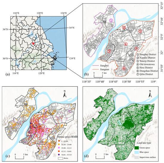
Figure 1.
Study area. (a) Location of main urban area of Nanjing; (b) administrative districts and street blocks; (c) spatial units of stress blocks and housing price points; (d) land use type.
2.2. Datasets
Three main datasets including WorldView-2 satellite images, mobile population, and POI (Point of Interest) data were used in this study.
The WorldView-2 satellite data with a spatial resolution of 0.5 m were used to generate high-resolution urban green space maps in this study. This dataset, acquired in 23 September 2022, were obtained from ESA’s Earth Online portal (https://earth.esa.int/eogateway/missions/worldview, accessed on 20 October 2025) [30,31]. With its high spatial resolution, multispectral imaging capabilities, and exceptional geometric accuracy, WorldView-2 data are the ideal data source for urban green space mapping.
The 24 h dynamic population data, sourced from Baidu Huiyan data (https://huiyan.baidu.com/), were used to extract dynamic population location change information in this study. This dataset, collected in hourly intervals, is measured in individuals. Data on 12 June 2021 (workday) and 10 October 2021 (weekend) were obtained and aggregated at the block scale. Baidu Huiyan divides the urban area into 200 × 200 m grids based on the Baidu Mercator coordinate system (bdmc09). For each grid, the system records the number of terminals that call the positioning SDK every hour and assigns a corresponding thermal value to the grid’s centroid. Consequently, each centroid has up to 24 hourly values representing different time intervals within a single day. The exposure to green space was calculated for both workdays and weekends in 24 h periods, including both daytime and nighttime periods. The multi-temporal population location data reflects effective dwell distributions around green space and outperforms social media check-in data in describing green space usage.
POI data include spatial information (such as latitude and longitude) and POI classification attributes (such as dining services, accommodation services, and companies) obtained through Baidu Maps (https://map.baidu.com/). POI data in 2022 were used to illustrate the characteristics of socioeconomic facilities in this study.
The road network data, sourced from the OSM (OpenStreetMap) website (https://www.openstreetmap.org/), were obtained in 2023. The urban road network, consisting of bidirectional four-lane roads, were used to divide the study area into 1410 blocks.
Housing price data in 2018 were used in this study, including the average listing price per unit area for residential units in communities, and were extracted from the real estate section of the Lianjia website (https://zh.lianjia.com). The housing price data in 2018 were utilized, as housing price may have been impacted by the COVID-19 pandemic. A total of 34,799 sample data points were collected, and 3198 data points were retained after excluding outliers.
The building height data were sourced from the “CNBH-10m” dataset, developed by the GC3S team [32] (https://zenodo.org/record/7827315), accessed on 21 October 2020. CNBH10m was used to extract the average building height of each block in this study.
2.3. Overall Framework
The overall framework of this study included four main steps (Figure 2), which were data collection and processing, spatiotemporal patterns of DRGE, green space exposure inequity assessment, and the impacts of built environment factors on DRGE. In the first step, we generated high-resolution urban green space maps from WorldView-2 satellite images. We aggregated the datasets such as Dynamic 24 h population data, built environment factors, housing prices, GDP, and other socioeconomic data, into 200 × 200 m grids. In the second step, we analyzed spatial patterns and temporal variations of DRGE during workday and weekend, by improving the population-weighted green space exposure model. In the third step, we divided the housing price blocks into four categories using quantiles, and compared the differences and equity of DRGE using the Palma ratio. In the fourth step, we used the XGBoost and SHAP methods to identify explanatory variables and calculated the relative importance of multiple urban environmental factors on DRGE.
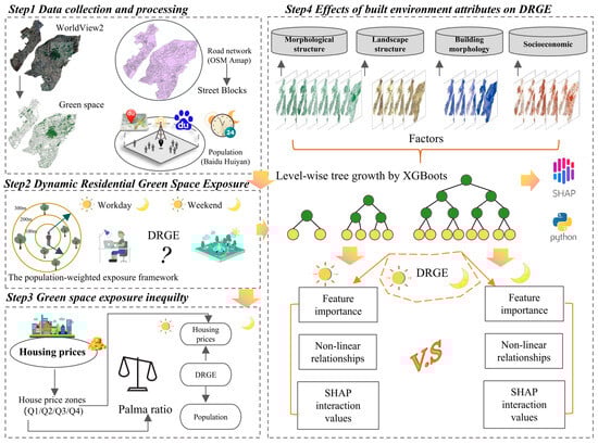
Figure 2.
Overall framework of this study.
To conduct a more detailed spatial analysis, street blocks were selected as the basic unit in our analysis. The choice of spatial unit not only aligns with the urban planning characteristics of Nanjing City but also helps to explore the issue of uneven distribution of green space resources at the street block level. These blocks were classified into four categories according to the housing price quartiles: Q1 (lowest-priced blocks), Q2 (lower-priced blocks), Q3 (higher-priced blocks), and Q4 (high-priced blocks).
2.4. Green Space Mapping Using Image Classification
We used the OBIC-GCN (Object-Based Image Classification with Graph Convolutional Network) model to generate the land use/land cover (LULC) map in this study. Object-Based Image Classification (OBIC), combined with high-resolution remote sensing imagery, is widely employed for urban land cover identification [13,33]. The OBIC-GCN is a new OBIC framework that leverages object relativity and combines truncated sparse Singular Value Decomposition (tSVD) for efficient object classification. The OBIC-GCN framework mainly consists of the following five steps: object generation, feature extraction, graph construction, tSVD dimensionality reduction, and OBIC-GCN model construction (Figure 3a). This framework enhances the accuracy and computational efficiency of the OBIC algorithm, significantly reducing training time, which has been validated in previous studies [33].
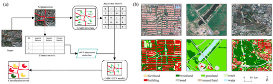
Figure 3.
Green space mapping in Nanjing City: (a) the OBIC-GCN model; (b) classification results in typical areas.
Utilizing this method, we interpreted WordView-2 satellite imagery at 0.5 m spatial resolution to generate green space maps, with strong classification performance (VOA: 0.923, OA: 0.909, Kappa: 0.862). Those metrics have been widely used in other high-accuracy land classification studies. Eight types of land use were classified, achieving good interpretation results with high accuracy (Figure 3b). Scrub, grassland, and woodland were further identified as green space.
2.5. Dynamic Green Space Exposure Mapping
Residents’ Green space Exposure (RGE) was calculated using the population size of each area as a weight, which accounts for the alignment between population distribution and the spatial location of green space [34,35]. Traditional RGE is estimated based on static population distribution data, which fail to capture population mobility across different time periods. Our method addressed this limitation by going beyond a supply-side perspective and emphasized demographic factors on the demand side, which is especially important in assessing equality and health impacts. In this study, we proposed a Dynamic Residential Green Space Exposure (DRGE) metric that incorporated a time dimension t. This enhanced model can reflect population dynamics at intra-daily, seasonal, and even inter-annual scales, enabling more accurate assessment of green space supply–demand characteristics across different temporal resolutions. The improved formula is presented as follows:
where DRGEt,d represents the dynamic residential green space exposure at time t and buffer distance d; t represents the time point; Pi,t represents the population size of the i th block at time t; represents the green space coverage of the ith block at time t in the buffer at distance d; N is the total number of grids for each blocks, and d represents the buffer extent. In this study, in response to the proposed 3–30–300 rule [36], the buffer size represented by d was set to 300 m.
Then we extracted the blocks with consecutive 2 h, 4 h, 6 h, and 8 h periods exceeding the DRGE average to compare the duration of residents’ green space exposure across different blocks, reflecting the supply and demand of green space.
2.6. Spatial Inequality of Green Space Exposure
In this study, we used the Palma ratio to reveal the inequality in DRGE between high- and low-priced housing blocks during daytime and nighttime. The Palma ratio is commonly used as an inequality index, measuring the income disparity between the wealthiest 10% of the population and the poorest 40%. In previous green space equality studies, the advantage of the Palma ratio over the Gini coefficient mainly lies in its intuitiveness, focus on extreme inequality, guidance for policy intervention, and robustness against outliers, as well as its greater adaptability and interpretability [2,34]. The Palma coefficient is calculated as follows:
where Palmai,t denotes the Palma coefficient of DRGE at time t and block i; DRGEi,t denotes the DRGE of block i at time t, and N is the total number of blocks. Here, the numerator sums DRGE over blocks in the top decile (90–100th percentile), while the denominator sums DRGE over blocks in the bottom four deciles (0–40th percentile). This follows the Palma coefficient convention and highlights inequality between the distribution’s upper and lower tails. The larger the Palma coefficient, the greater the inequality [2].
2.7. Model and Built Environment Factors Selection
2.7.1. XGBoost and Model Interpretation with SHAP
In this study, we employed the XGBoost (eXtreme Gradient Boosting) model to explore the impacts of built environment factors on DRGE across different temporal periods. The XGBoost model, a kind of machine learning regression modeling, offers a novel approach for exploring nonlinear relationships between built-up environments and green space exposure. XGBoost demonstrates several key advantages: higher predictive accuracy, greater modeling flexibility, enhanced overfitting prevention, and superior handling of missing values [37,38]. To better understand the effects of various factors on localized DRGE, this study also used SHAP (SHapley Additive exPlanation) to enhance model interpretability. SHAP is an advanced interpretive framework based on Shapley values from cooperative game theory, which quantifies the contribution of each feature to machine learning model predictions through importance scores. These scores effectively capture both positive and negative impacts of individual features on model outcomes. This method offers unique advantages in explaining complex interactions between model features and has proven particularly valuable for understanding multifaceted environmental relationships. The Shapley value for feature i is calculated using the following formula:
where ∅i represents the contribution of the feature i, N denotes the set with n features, and f(S∪) and f(S) represent the model results with or without the feature i.
In this study, the mean squared error (MSE), mean absolute error (MAE), R-square (R2), root mean squared error (RMSE), and mean absolute percentage error (MAPE) were used to evaluate the performance of the XGBoost model [39].
2.7.2. Selected Built Environment Factors
Twenty built environment factors were selected and extracted in this study, including 2D and 3D environment factors, and socioeconomic factors. Cities represent complex social–ecological systems characterized by intricate interactions between built environments and human activities. Given this complexity, it is essential to quantify the effects of the built environment on the DRGE [40]. In this study, we used a multi-dimensional approach encompassing three key aspects: (1) 2D spatial characteristics, including green space morphological structure and landscape pattern indicators; (2) 3D urban morphology, represented by building-related indicators; and (3) socioeconomic development indicators, including population density, POI mix degree, distance to parks (DTP), and distance to transportation (DTT).
We employed Morphological Spatial Pattern Analysis (MSPA) to examine the spatial connectivity of green space and characterize its morphological patterns [41]. The MSPA method classified green space within the study area as foreground elements, with all other land cover types designated as background. Based on their structural characteristics, green space was categorized into seven distinct morphological types, including core, edge, perforation, bridge, ring, branch, and island area. Subsequently, we calculated the proportional composition of each MSPA class within individual blocks. The percentage share of each morphological element relative to the total land area was then used as indicator representing the seven morphological dimensions influencing the DRGE.
where Pi represents the proportion of different MSPA classes in the buffer; Si represents the area of different MSPA classes in the buffer, and S represents the total area of all MSPA classes in the buffer. GuidosToolbox 3.0 was used to identify the morpho-spatial pattern of green space.
Four landscape metrics were selected to measure the spatial pattern of green space, which were Percent of Landscape (PLAND), Largest Patch Index (LPI), Aggregated Index (ED), and Mean Patch Shape index (SHAPE_MN). These factors were calculated using Fragstats 4.2 software.
Building Density (BD), Average Building Height (ABH), Floor Space Index (FSI), and Sky View Factor (SVF) were calculated to represent 3D characteristics of the built environment. The SVF is the maximum angle of the sky visible from the ground between two buildings, representing the relationship between building height and spacing. The SVF value ranges from [0, 1], where a value of 0 indicates the sky is completely blocked by obstacles relative to the ground, and a value of 1 means the sky is completely unobstructed [27,42]. The building footprint area is derived from high-resolution imagery extraction. The following formulas are used for calculation:
where F is the total floor area above ground; Af is the area of the urban plot; B is the base area of the building above ground, and L is the number of building floors.
Population density, POI mix degree, distance to parks, and distance to transportation facilities were calculated for the block [27]. The entropy of the secondary category of location of POIs within a block was used to characterize the functional diversity of POIs. The larger the entropy value of the secondary category, the greater the diversity of the distribution of the various types of accessible facilities on the street; the smaller the entropy value, and the lower the POI mix degree [27]. The formula is shown as follows:
where POImixusedi is the POI mix degree of block i; pij is the proportion of the number of type j POIs in block i to the total number of POIs in the block, and A is the number of POI types in the block. We collected POIs from the following perspectives: transportation (subways, bus stations, etc.), education (primary and middle schools), healthcare (top-ranked hospitals), leisure (parks), shopping (shopping malls), and other living facilities (restaurants, banks, etc.).
Before model training, we used the Variance Inflation Factor (VIF) test to assess multicollinearity among the explanatory variables. Severe multicollinearity is typically indicated by a VIF threshold greater than 10. No multicollinearity was found among the indicators in our results. Table 1 provides the indicator definitions and the results of the collinearity diagnostics.

Table 1.
Indicators and collinearity diagnosis.
3. Results
3.1. Spatiotemporal Patterns of Green Space Exposure
The average DRGE on the weekend was higher than that on a workday, with values of 0.346 and 0.231, respectively. In terms of diurnal variation, the DRGE value decreased between 00:00 and 06:00. After 06:00, the exposure value gradually increased until 18:00, after which it fluctuates and decreases (Figure 4a). The number of blocks with a DRGE value below 0.2 on workdays was significantly higher than on weekends, accounting for nearly 40% of the total (Figure 4b). In a street block with higher DRGE, residents were more likely to access green space on the weekend, reflecting a better supply–demand effect of green space.

Figure 4.
Diurnal variations of DRGE on workdays and weekends. (a) The 24 h average DRGE on workdays and weekends; (b) histogram of DRGE on workdays and weekends; (c) the 24 h average DRGE across four housing price blocks; (d) standard deviation across four housing price blocks.
Significant patterns of DRGE across four diverse housing price blocks were observed during 24 h on weekends and workdays, with higher-priced blocks having better supply and demand of green space and being served for longer periods. Mean DRGE on weekends was about 1.5 times higher than on workdays. On weekends, from 7:00 to 12:00, the mean DRGE value in high-priced blocks was 1.8 times higher than in low-priced blocks. Specifically, the DRGE value in Q4 (high-priced blocks) was approximately 0.282 after 19:00, which was about two times higher than that in Q1 (low-priced blocks at 0.134). This indicated that residents in high-priced blocks have access to more abundant green space during the evening. In Q2 (lower-priced blocks), around 32% of blocks in the area faced a serious supply–demand imbalance between 12:00 and 17:00 on workdays, with a value of approximately 0.142. In high-priced areas, the DRGE value on weekends, especially between 7:00 and 15:00, is around 0.25, and the likelihood of residents in Q3 (higher-priced blocks)/Q4 accessing green space was close to 0.3 (Figure 4c).
The variation of the standard deviation of DRGE in four housing price blocks reflected the degree of balance between supply and demand of green space in different time periods (Figure 4d). In high-priced blocks, the standard deviation remains stable for most of the time, while in low-priced blocks, the standard deviation fluctuates significantly between daytime and nighttime. The standard deviation in high-priced blocks (Q3 and Q4) was approximately 0.102 during daytime, and from 0.10 to 0.109 during nighttime. In contrast, the standard deviation values for both daytime and nighttime in low-priced blocks varied considerably, ranging from 0.113 to 0.128. Therefore, the standard deviation for high-priced blocks was about 0.01 to 0.02 lower than that of low-priced blocks.
There are significant differences in the duration of green space exposure across blocks (Figure 5). The proportion of high-priced blocks (with durations exceeding 8 h) on weekends was higher than on workdays, with more than 68% of higher- and high-priced blocks (Q3/Q4) enjoying better green space supply and demand services during weekend nighttime. During workday daytime and on weekend evenings, the proportion of Q4 blocks with exposure durations exceeding 6 h was much higher than that of other blocks, with proportions exceeding 40%. Furthermore, the proportion of mid-to-low-priced blocks (Q1/Q2) with a duration of 2 to 4 h remains high, exceeding 30%. In contrast, mid-to-high-priced blocks (Q3/Q4) account for about 25%.
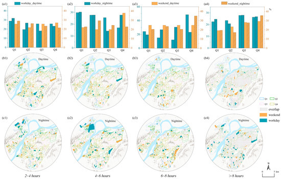
Figure 5.
Spatial patterns of DRGE duration in housing price blocks: (a1–a4) Percentage of the number of blocks on workdays and weekends during daytime and nighttime for residents’ exposure to green space; (b1–b4) spatial patterns of green space exposure across blocks during daytime on workdays and weekends; (c1–c4) spatial patterns of green space exposure across during nighttime on workdays and weekends.
Regarding spatial patterns, Jiangnan demonstrates a superior green space supply duration compared to Jiangbei overall, with high-value continuous supply areas concentrated in affluent districts such as Xianlin and the Zhongshan Scenic Area (Figure 5b,c). This spatial differentiation aligns with population density variations in commercial and residential zones, while disparities in large green space distribution further intensify regional imbalances in residents’ green space accessibility. These patterns reflect the dynamic relationship between green space supply and demand in response to resident mobility shifts.
3.2. Inequality of Green Space Exposure
The Palma coefficients on workdays and weekends were 0.442 and 0.533, respectively, indicating that inequality in DRGE was more pronounced on the weekend than on the workday. Although overall green space exposure on weekend was higher than that on workday, the disparity between blocks with high and low green space exposure was greater on the weekend compared to that on workday.
As house prices increased, the DRGE values became larger, and the equality of green space supply and demand improved (Table 2). The Q2 blocks (lower house prices) had the most severe inequities in green space supply and demand, with an average Palma ratio of over 0.445. These blocks were constrained by working hours and green space resources and have even larger gaps in Palma ratios. The weekend nighttime tended to face more severe inequalities, with a Palma ratio of 0.497. This inequality diminished as house prices increased. The average Palma ratio in Q4 blocks (highest house prices) across the two daytime dates was 0.383, which is slightly lower than 0.4, indicating relatively lower inequalities in the supply and demand for green space. When considering all time periods, the overall average Palma ratio was 0.386, confirming that high-priced areas generally experience a more balanced distribution of green space availability and use. In addition, the Palma ratios difference between daytime and nighttime was larger in Q3 and Q4 compared to Q1 and Q2. This reflected the fact that in high-priced areas, the Palma ratio difference between daytime and nighttime was bigger. Specifically, in high-price areas, the daytime inflow of workers and visitors increases both the population size and diversity, thus reducing inequality, while nighttime conditions reflect a more affluent and homogeneous resident population, resulting in higher Palma ratios and green space exposure.
Table 2.
Palma coefficient values in four house price blocks.
A significant positive correlation between house prices and distribution of green space was confirmed (Figure 6). Residents in higher-priced housing areas tend to have slightly higher green space exposure. In contrast, residents in areas with low housing prices had limited access to green spaces on the weekend during both daytime and nighttime, reflecting the uneven distribution of green space. For example, in the Q2 block, with the housing price range of CNY 10,000 to CNY 22,000 and the population from 1000 to 1300, had a slightly higher DRGE than Q1 (about 0.332), indicating that residents have more access to green space during the daytime. In the Q4 block, with the house price ranging from CNY 60,000 to CNY 70,000 and the population from 850 to 1250, had a higher exposure to residents’ green space, mainly concentrated in the range of 0.4 to 0.5, suggesting that residents in high-priced areas enjoy more green space resources. During the nighttime, the DRGE in these areas did not change much and remained around 0.4, suggesting that residents in high-priced blocks have a more balanced exposure to green space both during the daytime and nighttime.
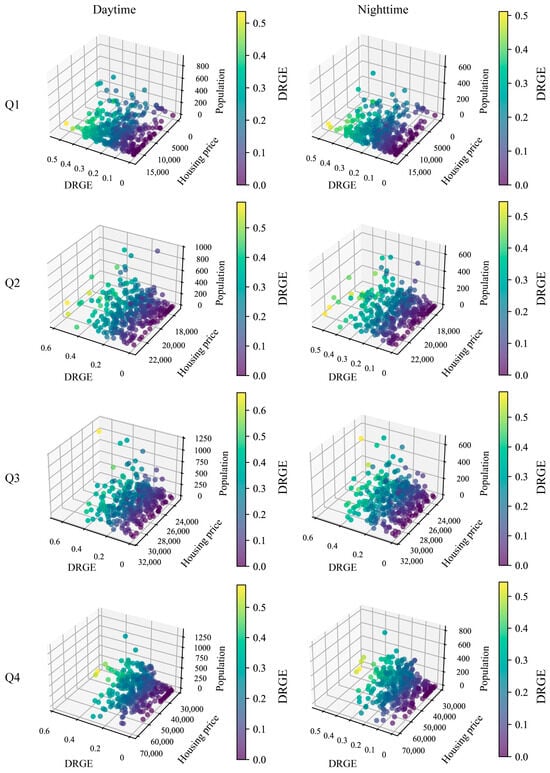
Figure 6.
Three-dimensional map of DRGE, housing prices, and population during the weekend daytime and nighttime.
3.3. Impacts of Built Environment Factors on Green Space Exposure
3.3.1. Variable Importance
During daytime, the DRGE was primarily influenced by three factors, including population, green space integrity, and transportation infrastructure. The mean |SHAP| values of the five most significant indicators were core proportion (0.285), edge (0.234), daytime population (0.215), connecting bridge (0.184), and distance to parks (DTP) (0.143) (Figure 7a,b). Good green space morphology and convenient transportation infrastructure promote efficient utilization of green spaces. Regularly shaped green space provides important recreational areas for citizens, especially being more fully utilized on weekends. The areas closer to parks have a better green space supply and demand balance. However, during nighttime, the top five influencing factors of DRGE were population (0.314), core area proportion (0.283), edge (0.263), distance to parks (0.174), and POI richness (0.137) (Figure 7c,d). Nighttime usage patterns were similar to those during daytime, but POI richness emerged as an important influencing factor. This indicates that nighttime activities are more centered on leisure and entertainment, especially in areas with a high density of POIs near regularly shaped green space, which attract more residents and increase people’s likelihood of green space exposure.
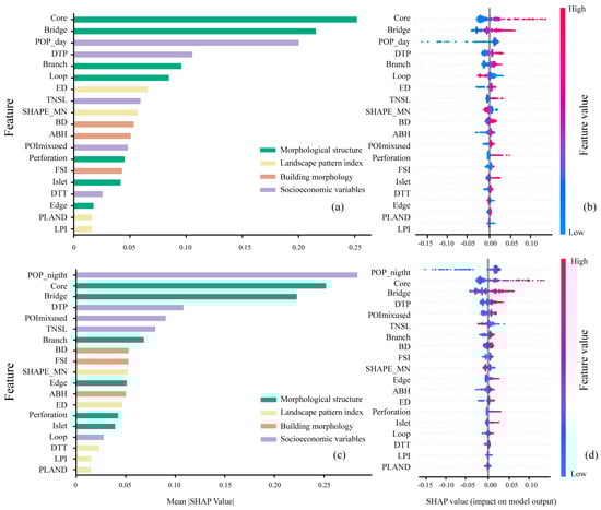
Figure 7.
Relative importance of variables. (a,b) The ranking based on importance and local interpretability diagram at daytime; (c,d) The ranking based on importance and local interpretability diagram at nighttime. Note: Each point on the plot corresponds to a SHAP value for an observation, with the color indicating the feature value (red for high, blue for low).
3.3.2. Nonlinear and Threshold Effects of Variables
We used SHAP dependency plots to elucidate complex nonlinear effects between variables, thereby clarifying the reasons behind the optimal value ranges of various variables at nighttime (Figure 8).
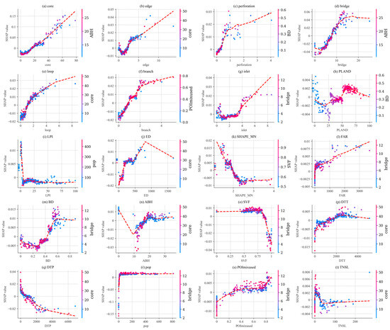
Figure 8.
SHAP dependence plots for built environment factors (red for high, blue for low).
- (1)
- Morphological structure. For most variables, higher values correspond to higher resident green space exposure. Increased core area proportion leads to increased green space exposure. Large population bases, dense buildings, and regularly shaped green space core areas with substantial size increase the probability of nearby residents’ contact with green spaces. For example, when core proportion exceeds 4.82%, we observed a positive correlation with resident green space exposure, and as the proportion of edge areas increases, the corresponding SHAP values slightly increase.
- (2)
- Landscape pattern. Within 25–70% PLAND, more green space typically means increased opportunities for residents’ exposure to green spaces, hence the positive correlation. When the total proportion of green space is too high or too low, it may lead to a negative correlation with exposure. Excessively high or low green space proportions may have more complex effects on exposure on weekend nights. When ED ≤ 850 m/ha, moderate increases in edge density may represent a reasonable distribution of green spaces, contributing to green space accessibility and diversity. When ED exceeds 850 m/ha, edge density may be too high, causing green space to be excessively divided or dispersed, affecting residents’ contact.
- (3)
- Building morphology. Building density reduces dynamic resident green space exposure. When BD exceeded 0.632, it showed a negative correlation. This finding was consistent with research on the relationship between BD and green space equality. Average height above 10 m showed a positive correlation with DRGE. These research results indicate that large green spaces may be distributed in areas with taller buildings, but such situations may occur in urban peripheral areas or new urban development zones. Urban greening efforts may also raise real estate values, causing urban blocks to face green justice issues. SVF exceeding 0.75 had a significant negative correlation with DRGE. In urban peripheral blocks with fewer green spaces, despite sparse buildings with fewer obstructions, the amount of green space provided to residents may be less.
- (4)
- Socioeconomic variables. Blocks with higher populations generally had lower levels of DRGE. When the distance to parks exceeded 1800 m, the DRGE showed a negative correlation. As the distance to parks increases, residents’ opportunities for accessing and the frequency of using green space decrease. Within the 0.4–0.8 range of POI mix, POI mix showed a clear negative correlation with DRGE. Green space may be compressed or occupied, leading to decreased residents’ exposure to green space.
3.3.3. Temporal Differentiation of SHAP Interaction
Interaction values among all variables were positive, but some interaction values varied slightly across different time periods during the weekend daytime and nighttime. The core proportion showed the most significant interaction among these variables (Figure 9). For instance, during daytime, the interaction value between core proportion and core proportion (0.722) was higher than other variables. These two regions collectively form the ‘connectivity’ of the green space ecological network, reflecting their important interactions in ecological functions, species movement, and green space utilization. The effective connection between core and bridge areas not only enhanced green network connectivity but also increased resident exposure to green spaces, indicating that these two elements have strong synergistic effects in ecological and environmental services during daytime, making green space more accessible and open to residents. During nighttime, the interaction value between core proportion and population (0.853) was the highest, suggesting that the combined effect of population concentration and green space area increases the probability of green space contact. Since residents often gather in city centers or near commercial, cultural, and public facility areas adjacent to core regions during this time, these areas with high proportions of green space and dense populations likely have higher green space exposure.
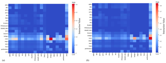
Figure 9.
SHAP interaction during (a) daytime and (b) nighttime.
4. Discussion
4.1. Green Space Exposure Patterns and Heat Exposure Inequality Across Housing Prices
In contrast to previous studies, this study proposed a metric that assesses Dynamic Residential Green Space Exposure (DRGE), which assesses differences in green space supply and demand in different housing price blocks (300 m buffer) from a population mobility perspective (workdays vs. weekends).
Results showed that residents are more likely to access green space on weekends compared to workdays, and the dynamic patterns of DRGE change under the constraints of the built environment at different times of the daytime and nighttime. These findings were consistent with the findings in previous study reported by Yoo and Roberts (2022) [21]. Typically, daytime activities primarily involve work, study, shopping, or socializing, which often entail long-distance commuting and spatial movement. In commuting or working places, the DRGE is mainly determined by the distribution of green space at destinations and along routes [45]. Nighttime activities, however, are predominantly concentrated around residential areas, with significantly reduced mobility among residents. The key determinant of DRGE during nighttime is the distribution of green space surrounding residential areas. Due to geographical variations in green space distribution across urban residential areas [4,46], blocks with insufficient green space configurations significantly reduce residents’ nighttime exposure.
Previous studies have highlighted the inequalities in green space exposure in the city, showing that residents in communities with higher housing prices are more likely to have access to abundant green spaces [47]. Residents in high-priced blocks can access green space more conveniently, with their DRGE significantly higher than that of residents in medium- and low-priced blocks during the weekend nighttime. Residents living in high-priced blocks often choose to engage in outdoor activities during the weekend, while potentially participating in leisure activities in green spaces near their homes at nighttime, enabling them to have more comprehensive contact with green spaces [28,48]. These high-quality green spaces are primarily concentrated in the Xinlin and Old Downtown districts, where housing prices are relatively higher than in peripheral urban areas [28]. The continuous improvement of the ecological environment has attracted middle- and high-income groups with better economic conditions, but it may simultaneously limit opportunities for disadvantaged groups to access green spaces. However, in low-priced blocks, the DRGE increases slightly during nighttime, suggesting that residents in these areas may disperse, choosing to walk or engage in entertainment activities that take them from their original residential areas toward regions with relatively abundant green spaces. Due to the large population base in these blocks, the overall level of DRGE remains low. Notably, the Palma ratio reaches its maximum value during nighttime in lower-priced blocks (Q2), indicating significant imbalances in green space acquisition in these blocks (Table 2), which further confirms that the impact of socioeconomic disparities on green space distribution within cities remains highly significant [49].
4.2. Nonlinear and Threshold Effects and Strategies for Improving Green Space Inequality
This study integrated the Object-Based Image Classification with Graph Convolutional Network (OBIC-GCN) model for the efficient extraction of urban green spaces at a fine scale, effectively reflecting the likelihood of residents’ access to these green spaces. It highlighted the significant role of high-resolution green space imagery in contemporary urban planning.
Our results indicated that the proportion of core areas in green space morphology is the dominant factor influencing DRGE and exhibits a significant positive correlation. Interestingly, when PLAND (percentage of green space) is in the range of 25–70%, increased green space typically means greater opportunities for residents to be exposed to green spaces, but this relationship demonstrates a clear threshold effect. This threshold finding can provide important reference guidance for future adjustments to green space proportions across different urban blocks. Additionally, urban building height and density primarily show negative correlations with DRGE. Similarly, our research calculations demonstrate that when residents’ distance from parks exceeds 1800 m, DRGE shows a significant negative correlation, suggesting that residents struggle to effectively access green spaces. These findings further supplement the research of Xu et al. (2018) [22], who reported that areas with higher population density are closely associated with better green space accessibility, while our study reveals more deeply the complex threshold effects of built environment factors.
Combining the findings of this study, we advocated that to achieve environmental equality in urban green space, the city planner should not only focus on the adjustment of the location and quantity of green space [7,50] but should also improve the planning and management of the urban green space system in light of the mobility pattern of the residents [45]. The threshold effect can effectively be leveraged to improve the inequity in DRGE. This aspect has not been thoroughly explored in previous studies. We further proposed targeted strategies for blocks with typical house prices based on the thresholds of variables (Figure 10).
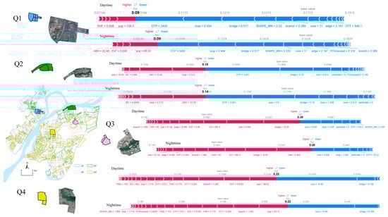
Figure 10.
Spatial distribution of DRGE and localized effects for representative cases of housing price blocks.
In Q1 (lowest-priced) blocks with housing prices below CNY 17,000 and an average DRGE value of around 0.152, SVF and POP are key factors. These areas are predominantly situated in the urban periphery, particularly in industrial zones along the river in downtown Jiangbei, characterized by open vistas but significant daytime population concentrations during the workday. However, these blocks suffer from distant and poorly connected green spaces. Considering that areas with higher green space coverage tend to have lower population densities and green space utilization, building more green spaces in low-density blocks has little impact on residents’ well-being. Given that the Overall Urban and Rural Spatial Plan of Nanjing City (2021–2035) designates this land for potential future development, direct policy intervention is essential to increase accessible green space availability. Therefore, such blocks can serve as evacuation zones for high-density populations with low-density green spaces. It is estimated that a PLAND threshold of 25–35% would be appropriate for these blocks.
In Q2 (lower-priced) blocks, a notable feature is that residents have more opportunities to access green spaces during the daytime, while the opposite is true at nighttime. Housing prices in Q2 blocks range from approximately CNY 17,000 to 23,000, and the Palma index exceeds 0.445, indicating significant inequality in green space access. This inequality is attributed to a high population density and low green space coverage, accompanied by significant population shifts between daytime and nighttime. The local SHAP index for Q2 indicates that accessibility factors (distance to parks) and population density contribute significantly to the highest inequalities in DRGE. Therefore, it is urgent to increase green space coverage to meet the demands of densely populated areas. It is estimated that a PLAND threshold of around 55–60% would more effectively satisfy the green space needs of these blocks.
In Q3 (higher-priced) blocks, green space configurations in these blocks demonstrate positive correlations with DRGE, reflecting superior accessibility and service provision capacity. These areas predominantly comprise newly developed urban districts, including the Hexi district and Xianlin district, which benefit from recent construction, robust infrastructure foundations, and continuous improvements. The abundance of large-scale green space has transformed these areas into premium green ‘assets’ within new urban developments. These districts experience pronounced daytime population peaks, likely attributed to commuting and recreational activities. There is an urgent need to regulate the value-added effect of large green patches (e.g., Zijin Mountain) while promoting their further integration with the population. In addition, attention should be paid to green expansion measures for high-density population blocks.
In Q4 (high-priced) blocks, residents have high exposure to green spaces, and the effects of green space supply and demand are favorable during both daytime and nighttime. For example, in the Old City District, around the Xuanwu Ming City Wall, these blocks have undergone updates and renovations, resulting in a reorganization of the social spatial structure. Although this area has high land value and overall good greening effects, the fragmentation of green space is significant. The district has a large population, and green space exposure is high on the weekend, making it an important place for residents to relax and tour. Research indicates that in most old urban areas in China, residents’ exposure to green space is higher during the daytime than at nighttime. Therefore, these types of blocks tend to adopt a ‘quantity-and-effect increase’ approach to alleviate the conflict between residential functions and green spaces. Solutions include three-dimensional greening initiatives, rooftop gardens, and other innovative approaches to compensate for limited ground-level green spaces. Intelligent urban planning can be used to improve the equality of urban green space.
4.3. Limitations and Future Work
There are several limitations to this study. First, our understanding of residents’ specific mobility patterns within blocks remain limited. Second, the population data derived from Baidu Huiyan big data are considerably lower than the actual urban population (including both permanent residents and floating population), suggesting that the actual green space exposure gap in Nanjing may be larger than estimated in this study, which urgently requires attention from local governments. Additionally, our analysis used blocks as the smallest statistical units, aggregated urban spatial factors into neighborhood-level averages, and employed housing price percentiles as classification standards—methods that need comparative analysis across different regional conditions.
Future research could explore the following directions: (1) Expanding green space exposure and inequality research across different population attributes. We used housing prices to reflect residents’ socioeconomic status without considering other relevant factors such as age, income, and gender. In the future, we can utilize tools like GPS tracking or OD distance methods to understand real-time green space supply and demand changes among different demographic groups (e.g., age, gender, occupation) within these blocks; (2) Integrating green space quality and considering exposure equality across different vegetation types and physical characteristics. Resident preferences (such as tree species preferences) are difficult to fully quantify. Taking into account residents’ inclinations would provide a more reasonable assessment of green space equality at different times. Future changes in green space and their relationship with exposure equality among residents of different attributes should be incorporated into discussions; (3) Comparing green space exposure and equality across different buffer ranges. This study specifically focuses on green space exposure within a 300 m range. However, the understanding of exposure equality within specific buffers around residents (e.g., 100 m, 500 m, or 1500 m) remains limited. Furthermore, existing research indicates that building morphology indices, street orientation, building dispersion, and other indicators correlate with block-level green space equality. In future work, we will incorporate more quantitative morphological indicators of block-level spatial layout to explore relationships between resident exposure and influencing factors at different scales. In addition, future studies should include data from multiple seasons to examine whether residents’ green space exposure preferences vary with seasonal changes.
5. Conclusions
This study generated hourly green space maps with a 0.5 m resolution and population maps. Based on these maps, a Dynamic Residential Green Space Exposure (DRGE) metric was proposed to examine the disparities in green space exposure experienced by residents across four different housing price blocks. Subsequently, the importance ranks and nonlinear effects of twenty building environment variables were investigated using XGBoost and SHAP methods.
The results demonstrated that the difference in daytime and nighttime DRGE values was significant, with the DRGE value being higher after 6:00 compared to the night. Mean DRGE on weekends was about 1.5 times higher than on workdays. Blocks with higher housing prices offer longer and more stable green space accessibility during the weekend compared to workdays, with over 68% of residents in higher-price blocks enjoying more than 8 h of green space during nighttime. Moreover, there was a significant imbalance in DRGE across different blocks, with lower-priced blocks exhibiting more pronounced inequality. The average Palma ratio for these blocks exceeded 0.445. Additionally, green space morphology, quantity, and population density in blocks were key factors influencing DRGE inequality. PLAND between 25 and 70% had a significant positive correlation with DRGE, while building density, height, and Sky View Factor (SVF) were negatively correlated with DRGE. These findings emphasize that leveraging the threshold effect to adjust the quantity of green space is crucial for improving the equality of DRGE. For lower-priced blocks (CNY 17,000–23,000), the PLAND threshold of 55–60% would effectively meet the green space demands of the residents.
This study provides an hourly high-resolution green space exposure mapping framework and demonstrates its utility for equality in urban green space analysis, which can also be applied to other cities where the mobility population and high-resolution remote sensing imagery data are available. At the same time, this framework is scalable and operational, making it applicable to different cities and having potential implications for urban planning, urban management, and public health. Future work should integrate population attribute data to further enhance the comprehensiveness of spatial and temporal differences and equality in DRGE mapping.
Author Contributions
Conceptualization: Y.W. and W.S.; data curation, Y.W.; formal analysis, Y.W. and J.H.; funding acquisition, Y.Y. and W.S.; methodology, Y.W. and J.H.; supervision, Y.Y., W.S. and J.H.; validation, W.S., Y.Y. and J.H.; visualization, Y.W. and W.S.; writing—original draft, Y.W.; writing—review and editing, W.S., Y.Y. and J.H. All authors have read and agreed to the published version of the manuscript.
Funding
This research was supported by the National Natural Science Foundation of China (Grant No. 42371397) and the Key Laboratory of Lake and Watershed Science for Water Security (Grant No. NKL2023-KP03).
Data Availability Statement
The data that support the findings of this study are available from the corresponding author upon reasonable request.
Acknowledgments
The authors would also like to express their sincere gratitude to colleagues and PhD students for their invaluable contributions to the data collection phase of this study.
Conflicts of Interest
The authors declare no conflicts of interest.
References
- Wolch, J.R.; Byrne, J.; Newell, J.P. Urban Green Space, Public Health, and Environmental Justice: The Challenge of Making Cities ‘Just Green Enough’. Landsc. Urban Plan. 2014, 125, 234–244. [Google Scholar] [CrossRef]
- Hu, J.; Zhang, F.; Qiu, B.; Zhang, X.; Yu, Z.; Mao, Y.; Wang, C.; Zhang, J. Green-Gray Imbalance: Rapid Urbanization Reduces the Probability of Green Space Exposure in Early 21st Century China. Sci. Total Environ. 2024, 933, 173168. [Google Scholar] [CrossRef]
- Zhang, J.; Cheng, Y.; Li, H.; Wan, Y.; Zhao, B. Deciphering the Changes in Residential Exposure to Green Spaces: The Case of a Rapidly Urbanizing Metropolitan Region. Build. Environ. 2021, 188, 107508. [Google Scholar] [CrossRef]
- Song, Y.; Chen, B.; Ho, H.C.; Kwan, M.P.; Liu, D.; Wang, F.; Wang, J.; Cai, J.; Li, X.; Xu, Y.; et al. Observed Inequality in Urban Greenspace Exposure in China. Environ. Int. 2021, 156, 106778. [Google Scholar] [CrossRef]
- Chang, F.; Huang, Z.; Liu, W.; Huang, J. A Novel Framework for Assessing Urban Green Space Equity Integrating Accessibility and Diversity: A Shenzhen Case Study. Remote Sens. 2025, 17, 2551. [Google Scholar] [CrossRef]
- Song, Y.; Huang, B.; Cai, J.; Chen, B. Dynamic Assessments of Population Exposure to Urban Greenspace Using Multi-Source Big Data. Sci. Total Environ. 2018, 634, 1315–1325. [Google Scholar] [CrossRef]
- Tian, D.; Wang, J.; Xia, C.; Zhang, J.; Zhou, J.; Tian, Z.; Zhao, J.; Li, B.; Zhou, C. The Relationship between Green Space Accessibility by Multiple Travel Modes and Housing Prices: A Case Study of Beijing. Cities 2024, 145, 104694. [Google Scholar] [CrossRef]
- Cheng, Y.; Wang, W.; Ren, Z.; Zhao, Y.; Liao, Y.; Ge, Y.; Wang, J.; He, J.; Gu, Y.; Wang, Y.; et al. Multi-Scale Feature Fusion and Transformer Network for Urban Green Space Segmentation from High-Resolution Remote Sensing Images. Int. J. Appl. Earth Obs. Geoinf. 2023, 124, 103514. [Google Scholar] [CrossRef]
- Yin, J.; Dong, J.; Hamm, N.A.S.; Li, Z.; Wang, J.; Xing, H.; Fu, P. Integrating Remote Sensing and Geospatial Big Data for Urban Land Use Mapping: A Review. Int. J. Appl. Earth Obs. Geoinf. 2021, 103, 102514. [Google Scholar] [CrossRef]
- Cao, Y.; Li, G.; Huang, Y. Spatiotemporal Evolution of Residential Exposure to Green Space in Beijing. Remote Sens. 2023, 15, 1549. [Google Scholar] [CrossRef]
- Chen, B.; Tu, Y.; Wu, S.; Song, Y.; Jin, Y.; Webster, C.; Xu, B.; Gong, P. Beyond Green Environments: Multi-Scale Difference in Human Exposure to Greenspace in China. Environ. Int. 2022, 166, 107348. [Google Scholar] [CrossRef] [PubMed]
- Wang, J.; Ma, A.; Zhong, Y.; Zheng, Z.; Zhang, L. Cross-Sensor Domain Adaptation for High Spatial Resolution Urban Land-Cover Mapping: From Airborne to Spaceborne Imagery. Remote Sens. Environ. 2022, 277, 113058. [Google Scholar] [CrossRef]
- Yang, R.; Qi, Y.; Zhang, H.; Wang, H.; Zhang, J.; Ma, X.; Zhang, J.; Ma, C. A Study on the Object-Based High-Resolution Remote Sensing Image Classification of Crop Planting Structures in the Loess Plateau of Eastern Gansu Province. Remote Sens. 2024, 16, 2479. [Google Scholar] [CrossRef]
- Cao, Y.; Li, Y.; Shen, S.; Wang, W.; Peng, X.; Chen, J.; Liao, J.; Lv, X.; Liu, Y.; Ma, L.; et al. Mapping Urban Green Equity and Analysing Its Impacted Mechanisms: A Novel Approach. Sustain. Cities Soc. 2024, 101, 105071. [Google Scholar] [CrossRef]
- Wang, W.; Cheng, Y.; Ren, Z.; He, J.; Zhao, Y.; Wang, J.; Zhang, W. A Novel Hybrid Method for Urban Green Space Segmentation from High-Resolution Remote Sensing Images. Remote Sens. 2023, 15, 5472. [Google Scholar] [CrossRef]
- Chen, K.; Wang, Y.; Huang, C.; Wang, J.; Li, S.L.; Guan, H.; Ma, L. GreenNet: A Dual-Encoder Network for Urban Green Space Classification Using High-Resolution Remotely Sensed Images. Int. J. Appl. Earth Obs. Geoinf. 2025, 142, 104709. [Google Scholar] [CrossRef]
- Wu, S.; Yu, W.; An, J.; Lin, C.; Chen, B. Remote Sensing of Urban Greenspace Exposure and Equality: Scaling Effects from Greenspace and Population Mapping. Urban For. Urban Green. 2023, 90, 128136. [Google Scholar] [CrossRef]
- Helbich, M. Toward Dynamic Urban Environmental Exposure Assessments in Mental Health Research. Environ. Res. 2018, 161, 129–135. [Google Scholar] [CrossRef]
- Lyu, F.; Zhang, L. Using Multi-Source Big Data to Understand the Factors Affecting Urban Park Use in Wuhan. Urban For. Urban Green. 2019, 43, 126367. [Google Scholar] [CrossRef]
- Chen, Y.; La Rosa, D.; Yue, W. Does Urban Sprawl Lessen Green Space Exposure? Evidence from Chinese Cities. Landsc. Urban Plan. 2025, 257, 105319. [Google Scholar] [CrossRef]
- Yoo, E.; Roberts, J.E. Static Home-Based versus Dynamic Mobility-Based Assessments of Exposure to Urban Green Space. Urban For. Urban Green. 2022, 70, 127528. [Google Scholar] [CrossRef]
- Xu, C.; Haase, D.; Pribadi, D.O.; Pauleit, S. Spatial Variation of Green Space Equity and Its Relation with Urban Dynamics: A Case Study in the Region of Munich. Ecol. Indic. 2018, 93, 512–523. [Google Scholar] [CrossRef]
- Lu, Y.; Kim, J.; Shu, X.; Zhang, W.; Wu, J. Confronting the Controversy over Neighborhood Effect Bias in Green Exposure: Using Large-Scale Multi-Temporal Mobile Signal Data. Landsc. Urban Plan. 2025, 253, 105222. [Google Scholar] [CrossRef]
- Zhang, X.; Chen, J.; Wang, H.; Yang, D. From Policy Synergy to Equitable Greenspace: Unveiling the Multifaceted Effects of Regional Cooperation upon Urban Greenspace Exposure Inequality in China’s Megacity-Regions. Appl. Geogr. 2025, 174, 103472. [Google Scholar] [CrossRef]
- Zhang, T.; Wang, L.; Hu, Y.; Zhang, W.; Liu, Y. Measuring Urban Green Space Exposure Based on Street View Images and Machine Learning. Forests 2024, 15, 655. [Google Scholar] [CrossRef]
- Gu, X.; Li, Q.; Chand, S. Factors Influencing Residents’ Access to and Use of Country Parks in Shanghai, China. Cities 2020, 97, 102501. [Google Scholar] [CrossRef]
- Doan, Q.C.; Ma, J.; Chen, S.; Zhang, X. Nonlinear and Threshold Effects of the Built Environment, Road Vehicles and Air Pollution on Urban Vitality. Landsc. Urban Plan. 2025, 253, 105204. [Google Scholar] [CrossRef]
- Yuan, F.; Wu, J.; Wei, Y.D.; Wang, L. Policy Change, Amenity, and Spatiotemporal Dynamics of Housing Prices in Nanjing, China. Land Use Policy 2018, 75, 225–236. [Google Scholar] [CrossRef]
- Huang, Y.; Hong, X.; Yao, X.; Yin, M. Which Characteristics Represent the Gentrification Affected by Parks? A Study Case in Nanjing, China. Ecol. Indic. 2024, 160, 111862. [Google Scholar] [CrossRef]
- Omarzadeh, D.; Karimzadeh, S.; Matsuoka, M.; Feizizadeh, B. Earthquake Aftermath from Very High-Resolution WorldView-2 Image and Semi-Automated Object-Based Image Analysis (Case Study: Kermanshah, Sarpol-e Zahab, Iran). Remote Sens. 2021, 13, 4272. [Google Scholar] [CrossRef]
- Tian, J.; Wang, L.; Li, X.; Gong, H.; Shi, C.; Zhong, R.; Liu, X. Comparison of UAV and WorldView-2 Imagery for Mapping Leaf Area Index of Mangrove Forest. Int. J. Appl. Earth Obs. Geoinf. 2017, 61, 22–31. [Google Scholar] [CrossRef]
- Wu, W.-B.; Ma, J.; Banzhaf, E.; Meadows, M.E.; Yu, Z.-W.; Guo, F.-X.; Sengupta, D.; Cai, X.-X.; Zhao, B. A First Chinese Building Height Estimate at 10 m Resolution (CNBH-10 m) Using Multi-Source Earth Observations and Machine Learning. Remote Sens. Environ. 2023, 291, 113578. [Google Scholar] [CrossRef]
- Zhang, X.; Tan, X.; Chen, G.; Zhu, K.; Liao, P.; Wang, T. Object-Based Classification Framework of Remote Sensing Images With Graph Convolutional Networks. IEEE Geosci. Remote Sens. Lett. 2022, 19, 8010905. [Google Scholar] [CrossRef]
- Cao, Y.; Li, G. Extensive Inequality of Residential Greenspace Exposure within Urban Areas in China. Sci. Total Environ. 2024, 948, 174625. [Google Scholar] [CrossRef] [PubMed]
- Wang, J.; Kwan, M.-P.; Xiu, G.; Peng, X.; Liu, Y. Investigating the Neighborhood Effect Averaging Problem (NEAP) in Greenspace Exposure: A Study in Beijing. Landsc. Urban Plan. 2024, 243, 104970. [Google Scholar] [CrossRef]
- Konijnendijk, C.C. Evidence-Based Guidelines for Greener, Healthier, More Resilient Neighbourhoods: Introducing the 3–30–300 Rule. J. For. Res. 2023, 34, 821–830. [Google Scholar] [CrossRef]
- Chen, T.; Guestrin, C. XGBoost. In Proceedings of the 22nd ACM SIGKDD International Conference on Knowledge Discovery and Data Mining, San Francisco, CA, USA, 13–17 August 2016; pp. 785–794. [Google Scholar]
- Li, Z. Extracting Spatial Effects from Machine Learning Model Using Local Interpretation Method: An Example of SHAP and XGBoost. Comput. Environ. Urban Syst. 2022, 96, 101845. [Google Scholar] [CrossRef]
- Wang, L.; Yin, H.; Li, Y.; Yang, Z.; Wang, Y.; Liu, X. Prediction of Microbial Activity and Abundance Using Interpretable Machine Learning Models in the Hyporheic Zone of Effluent-Dominated Receiving Rivers. J. Environ. Manag. 2024, 357, 120627. [Google Scholar] [CrossRef]
- Grant, A.; Millward, A.A.; Edge, S.; Roman, L.A.; Teelucksingh, C. Where Is Environmental Justice? A Review of US Urban Forest Management Plans. Urban For. Urban Green. 2022, 77, 127737. [Google Scholar] [CrossRef]
- Chen, J.; Kinoshita, T.; Li, H.; Luo, S.; Su, D. Which Green Is More Equitable? A Study of Urban Green Space Equity Based on Morphological Spatial Patterns. Urban For. Urban Green. 2024, 91, 128178. [Google Scholar] [CrossRef]
- Lin, J.; Qiu, S.; Tan, X.; Zhuang, Y. Measuring the Relationship between Morphological Spatial Pattern of Green Space and Urban Heat Island Using Machine Learning Methods. Build. Environ. 2023, 228, 109910. [Google Scholar] [CrossRef]
- Guan, J.; Wang, R.; Berkel, D.V.; Liang, Z. How Spatial Patterns Affect Urban Green Space Equity at Different Equity Levels: A Bayesian Quantile Regression Approach. Landsc. Urban Plan. 2023, 233, 104709. [Google Scholar] [CrossRef]
- Hu, P.; Wang, A.; Yang, Y.; Pan, X.; Hu, X.; Chen, Y.; Kong, X.; Bao, Y.; Meng, X.; Dai, Y. Spatiotemporal Downscaling Method of Land Surface Temperature Based on Daily Change Model of Temperature. IEEE J. Sel. Top. Appl. Earth Obs. Remote Sens. 2022, 15, 8360–8377. [Google Scholar] [CrossRef]
- Zheng, L.; Kwan, M.-P.; Liu, Y.; Liu, D.; Huang, J.; Kan, Z. How Mobility Pattern Shapes the Association between Static Green Space and Dynamic Green Space Exposure. Environ. Res. 2024, 258, 119499. [Google Scholar] [CrossRef] [PubMed]
- Dong, Q.; Zeng, P.; Long, X.; Peng, M.; Tian, T.; Che, Y. An Improved Accessibility Index to Effectively Assess Urban Park Allocation: Based on Working and Residential Situations. Cities 2024, 145, 104736. [Google Scholar] [CrossRef]
- Yuan, Y.; Tang, S.; Guo, W.; Zhang, J. Spatiotemporal Dynamics and Driving Factors of Green-Blue Space in High-Density Cities: Evidence from Central Nanjing. Ecol. Indic. 2024, 160, 111860. [Google Scholar] [CrossRef]
- Tang, Y.; Xiao, W.; Yuan, F. Evaluating Objective and Perceived Ecosystem Service in Urban Context: An Indirect Method Based on Housing Market. Landsc. Urban Plan. 2025, 254, 105245. [Google Scholar] [CrossRef]
- Wu, L.F.; Kim, S.K. Does Socioeconomic Development Lead to More Equal Distribution of Green Space? Evidence from Chinese Cities. Sci. Total Environ. 2021, 757, 143780. [Google Scholar] [CrossRef]
- Xiao, Y.; Wang, Z.; Li, Z.; Tang, Z. An Assessment of Urban Park Access in Shanghai—Implications for the Social Equity in Urban China. Landsc. Urban Plan. 2017, 157, 383–393. [Google Scholar] [CrossRef]


Disclaimer/Publisher’s Note: The statements, opinions and data contained in all publications are solely those of the individual author(s) and contributor(s) and not of MDPI and/or the editor(s). MDPI and/or the editor(s) disclaim responsibility for any injury to people or property resulting from any ideas, methods, instructions or products referred to in the content. |
© 2025 by the authors. Licensee MDPI, Basel, Switzerland. This article is an open access article distributed under the terms and conditions of the Creative Commons Attribution (CC BY) license (https://creativecommons.org/licenses/by/4.0/).