Article

IAASNet: Ill-Posed-Aware Aggregated Stereo Matching Network for Cross-Orbit Optical Satellite Images

1
School of Earth Sciences and Resources, China University of Geosciences (Beijing), Beijing 100083, China
2
School of Remote Sensing and Information Engineering, Wuhan University, Wuhan 430079, China
*
Author to whom correspondence should be addressed.
Remote Sens. 2025, 17(21), 3528; https://doi.org/10.3390/rs17213528
Submission received: 6 September 2025 / Revised: 15 October 2025 / Accepted: 23 October 2025 / Published: 24 October 2025

Highlights

What are the main findings?
  • An ill-posed-aware stereo matching framework integrates monocular depth estimation with adaptive geometry fusion to improve disparity estimation in ill-posed regions of cross-orbit images.
  • An enhanced mask augmentation strategy improves robustness to occlusions, weak textures, and imaging challenges in cross-orbit satellite conditions.
What is the implication of the main finding?
  • Achieving 5.38% D1-error and 0.958px EPE on the corrected US3D dataset, with significant accuracy gains in ill-posed regions.
  • Enhancing generalization ability, enabling more reliable cross-orbit remote sensing applications.

Abstract

Stereo matching estimates disparity by finding correspondences between stereo image pairs. Under ill-posed conditions such as geometric differences, radiometric differences, and temporal changes, accurate estimation becomes difficult due to insufficient matching information. In remote sensing imagery, such ill-posed regions are more common because of complex imaging conditions. This problem is particularly pronounced in cross-track satellite stereo images, where existing methods often fail to effectively handle noise due to insufficient features or excessive reliance on prior assumptions. In this work, we propose an ill-posed-aware aggregated satellite stereo matching network, which integrates monocular depth estimation with an ill-posed-guided adaptive aware geometry fusion module to balance local and global features while reducing noise interference. In addition, we design an enhanced mask augmentation strategy during training to simulate occlusions and texture loss in complex scenarios, thereby improving robustness. Experimental results demonstrate that our method outperforms existing state-of-the-art approaches on the US3D dataset, achieving a 5.38% D1-error and 0.958 pixels endpoint error (EPE). In particular, our method shows significant advantages in ill-posed regions. Overall, the proposed network not only exhibits strong feature learning ability but also demonstrates robust generalization in real-world remote sensing applications.

1. Introduction

Stereo matching estimates disparity from rectified image pairs to recover three-dimensional geometry and is widely used in remote sensing for generating DSMs or point clouds, providing essential data for urban modeling, mapping, and disaster monitoring [1,2,3]. In recent years, cost-volume–based approaches built upon convolutional neural networks (CNNs) have achieved remarkable progress in stereo matching tasks, where feature extraction, matching cost computation, regularization, and disparity regression are jointly optimized [4,5,6]. However, under ill-posed conditions such as geometric inconsistencies, radiometric differences, and temporal variations in cross-orbit satellite remote sensing scenarios, the stability and accuracy of current disparity estimation algorithms remain difficult to guarantee.
On one hand, stereo matching in cross-orbit satellite imagery must not only address conventional ill-posed regions areas inherently challenging due to insufficient local distinctiveness and poor matching consistency, but also contend with significantly aggravated difficulties introduced by cross-orbit imaging conditions. Traditional stereo matching becomes substantially more complex: occlusions become more frequent and intricate due to the widened baseline; repetitive textures are more prone to mismatches owing to variations in viewing angles; disparity discontinuities exhibit sharper depth jumps; and weakly textured regions suffer further degradation in feature representation and matching consistency due to differences in resolution and illumination. Meanwhile, cross-orbit imaging introduces a fundamental challenge rarely encountered in conventional stereo matching—temporal variation. Since the left and right images may be captured at different times, objects on the ground may undergo geometric changes (e.g., new constructions or demolitions) or radiometric alterations (e.g., vegetation growth, seasonal shifts). Consequently, theoretically corresponding points may have shifted or even ceased to exist in the physical world. This characteristic renders pixel-level matching methods that rely on appearance consistency inherently fragile, posing one of the most distinctive and formidable challenges in cross-orbit satellite stereo matching.
On the other hand, complex occlusion patterns, extensive textureless areas, and structural deformations commonly observed in real remote sensing scenes are often insufficiently represented in existing training datasets. The acquisition of cross-track stereo data is costly and difficult to annotate, resulting in a limited dataset size and incomplete coverage of diverse ill-posed conditions. Consequently, models trained on such datasets tend to exhibit instability and weak generalization when encountering unseen or highly variable real-world scenarios during inference.
In this paper, we propose an ill-posed-aware aggregated stereo matching framework. Specifically, we design an Ill-posed-guided Adaptive Aware Geometry Fusion (IAGF) module, which generates ill-posed and well-posed features via a left-right consistency mask from the initial disparity, and adaptively fuses monocular and stereo geometric features to iteratively refine disparity estimation. Our method preserves accuracy in well-posed regions while enabling structurally-aware, context-dependent reconstruction in ill-posed areas, thereby overcoming the limitations of local matching failures. In addition, we introduce an Enhanced Mask Augmentation (EMA) strategy that combines random regular erasing with key-point-based masking, effectively enhancing the model’s discriminative ability in low-texture, occluded, and variant regions, and improving its adaptability to cross-temporal and cross-sensor variations in remote sensing imagery.
The main contributions of this work are as follows:
  • We construct an ill-posed-aware aggregation network that incorporates monocular depth, where ill-posed regions are identified via left-right consistency masks and used as constraints to generate aware features. By adaptively weighting and aggregating aware and geometric features, the network comprehensively improves disparity estimation accuracy.
  • We propose an enhanced mask-based data augmentation training strategy (EMA) for remote sensing imagery, which integrates random erasing and key-point mask augmentation to effectively improve the robustness and generalization capability of the model in complex scenarios.
  • Our method achieves state-of-the-art performance on the US3D cross-orbit satellite stereo matching dataset, with particularly remarkable improvements in ill-posed regions.
The structure of this paper is as follows: Section 2 reviews related work. Section 3 elaborates on the proposed methodology in detail. Section 4 presents the experimental setup, reports the findings, and provides a preliminary analysis. Section 5 evaluates the effectiveness and performance of the proposed method through ablation studies and efficiency analysis. Section 6 summarizes the paper and outlines potential directions for future research

2. Related Work

2.1. Deep Learning for Stereo Matching

In recent years, deep neural networks have been widely applied to stereo matching tasks. Early works such as GCNet [7] first introduced the concatenation of left–right image features to construct a 4D cost volume, which retains richer contextual information. Subsequently, a series of approaches [8,9,10,11] adopted similar core architectures, focusing on optimizing the cost-volume in conjunction with 3D convolutional networks for feature aggregation.
PSM-Net [12] exploited a spatial pyramid pooling module to extract multi-scale features and employed a stacked hourglass architecture during cost aggregation to refine the initial cost volume. GwcNet [11] proposed the group-wise correlation strategy, which effectively combines correlation-based and concatenation-based cost volumes. GA-Net [13] further reinforced the cost-volume by integrating both local and global aggregation strategies. IGEV [14] introduced the Geometry Encoding Volume to jointly model geometric structures and contextual information. UGC-Net [15] developed an uncertainty-guided disparity estimation and refinement strategy, where disparity optimization is achieved by adjusting cost volume weights and aggregating contextual information. More recently, [16] proposed a self-refinement mechanism for cost volumes by jointly optimizing left–right and intra-view (left–left) cost representations.
Although these methods have alleviated the ill-posed problem to some extent, they remain heavily dependent on cost-volume optimization. In particular, reliable correspondences are nearly unattainable in textureless or severely occluded regions. Without image-level interventions, these approaches still suffer from inherent ambiguities and uncertainties that limit disparity accuracy.

2.2. Disparity Optimization in Ill-Posed Regions

To address the challenges posed by ill-posed regions, vision-based approaches primarily exploit structural or semantic cues from images, with several studies [17,18,19,20] attempting to incorporate priors as guidance. EdgeStereo [21] incorporated edge cues to regularize disparity estimation, while S2Net [22], S3Net [23], and [24] employed semantic segmentation outputs for semantic guidance, effectively improving matching in textureless regions. However, edge and semantic cues primarily provide object-level information, which remains insufficient for fine-grained, pixel-level depth perception.
Another research direction, represented by multimodal spectral methods, seeks to enhance feature representation by incorporating spectral information beyond the visible range. Multimodal spectral stereo matching approaches, such as those using hyperspectral or multispectral data, introduce high-dimensional and cross-modal information to address ill-posed problems from a complementary perspective by enriching the discriminative power of features through additional information channels beyond RGB color. Representative studies [25,26] follow this idea, utilizing the rich spectral characteristics of multimodal data to improve the robustness of cross-modal stereo matching. However, these methods typically rely on a crucial assumption that consistent spectral characteristics exist between the left and right views. In cross-track satellite imagery, this assumption is often invalid due to significant temporal variations and changes in the spectral properties of ground objects. Consequently, the direct application of such methods to cross-track satellite stereo matching remains highly limited.
Moreover, most of the aforementioned methods based on semantic guidance and multi-modal spectroscopy adopt a multi-task network architecture, where semantic segmentation or spectral feature extraction is typically designed as an auxiliary task and jointly trained with stereo matching. However, this paradigm heavily relies on large-scale, high-quality, and precisely aligned multi-task annotated data for joint supervision, such as pixel-level disparity, semantic labels, and spectral information. In practical scenarios, particularly in satellite remote sensing, acquiring such comprehensive, balanced, and strictly cross-modal registered datasets is costly and extremely challenging. The scarcity of datasets and limitations in annotation quality make it difficult to adequately train such multi-task networks, thereby restricting their model generalization capability and performance in real-world applications.
To enable more refined feature utilization, STTR [27] replaced conventional cost volume construction with a sequence-to-sequence pixel matching framework based on positional encoding, attention mechanisms, and context aggregation, thereby enhancing confidence estimation. More recently, GOAT [28] introduced an occlusion-aware global aggregation strategy that significantly improves disparity accuracy in occluded regions.
Meanwhile, several studies [29] have explored monocular depth estimation as a complementary source of information to enhance stereo matching. For instance, [30] integrated a monocular depth branch to mitigate issues in textureless regions, while [31] transferred structural information from monocular networks into stereo frameworks to strengthen structural understanding. In [32], a novel cost volume design fused monocular depth with RGB features, improving robustness via cosine-grouped correlations. FoundationStereo [33] leveraged large-scale synthetic datasets and incorporated priors from Depth Anything V2 [34] to establish a foundation model for stereo matching, reducing the domain gap between synthetic and real data. DEFOM [35] integrated monocular depth models into a recurrent stereo framework. These approaches, being less reliant on pixel-level correspondence, provide stronger structural awareness and partial depth compensation. Nevertheless, insufficient constraints often lead to scale drift and structural distortions. Monster [36] proposed a dual-branch architecture combining monocular and stereo information to calibrate global scale shifts and perform bidirectional iterative optimization, thereby alleviating drift and distortion. However, naive fusion of monocular depth can introduce redundant noise, potentially weakening stereo feature representations.
In this work, we propose IAASNet that explicitly addresses both the limitations of stereo matching networks in correspondence-free regions and the potential noise introduced by monocular depth fusion. Our method generates aware features and adaptively integrates them with monocular and stereo geometric features for fine-grained and efficient feature aggregation. Furthermore, by employing enhanced mask augmentation to dynamically simulate occlusions and missing regions during training, our framework enables the network to learn stronger completion and generalization capabilities. Compared with prior approaches that rely solely on specific priors or direct monocular fusion, our method achieves superior accuracy in ill-posed regions, particularly under occlusions and geometric deformations.

3. Materials and Methods

3.1. Overall Framework

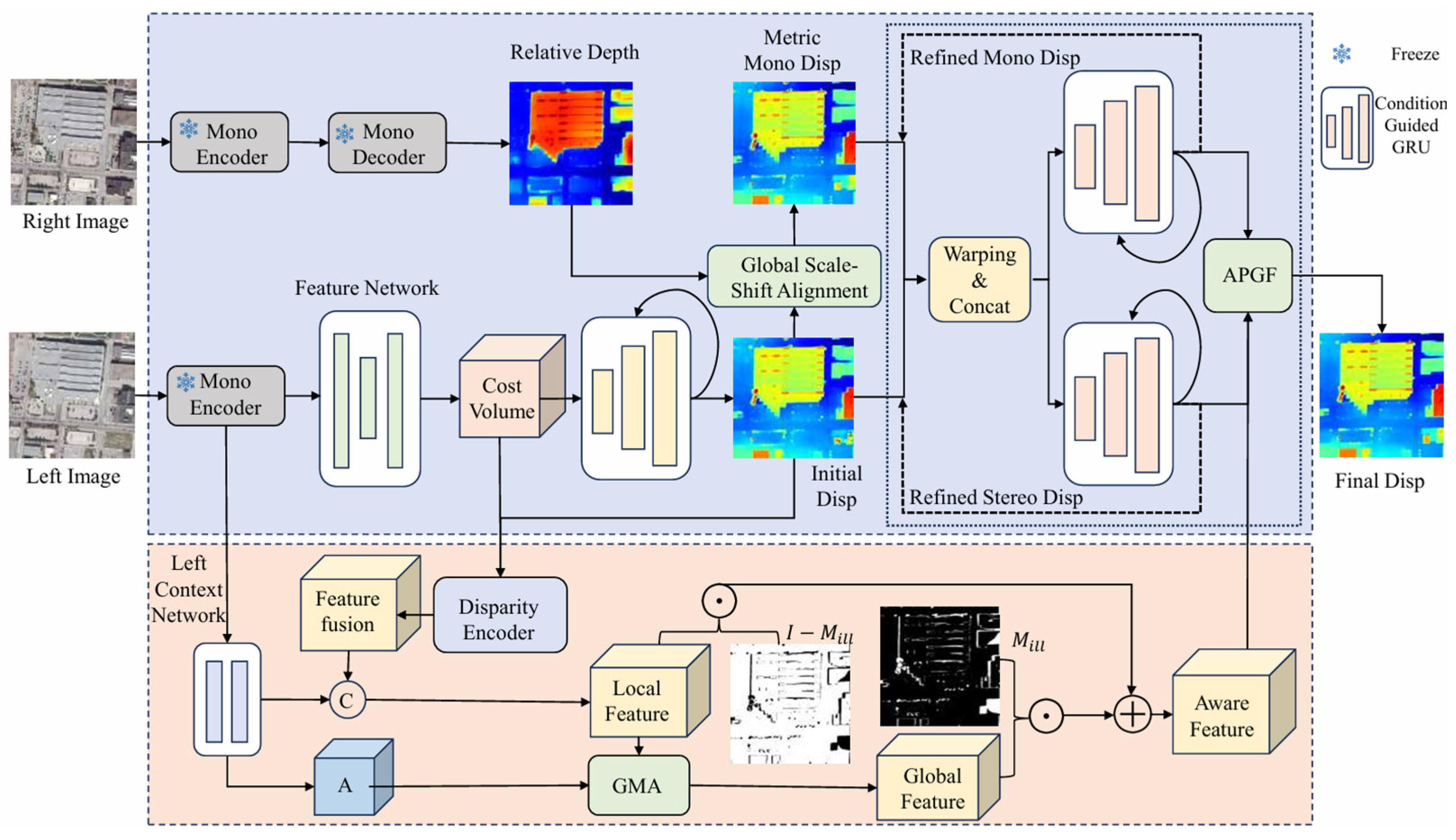
Figure 1 presents the architecture of Monster, a stereo matching network integrated with monocular depth estimation. Building upon Monster, Figure 2 illustrates the overall architecture of our proposed model, which incorporates an Ill-posed-guided Adaptive Aware Geometry Fusion (IAGF) module. This module refines the final disparity prediction by effectively fusing ill-posed-aware features with monocular and stereo geometric features. We first describe the architecture of Monster, and then introduce our proposed network in detail.

3.2. Marry Monodepth to Stereo Matching

3.2.1. Monocular and Stereo Branches

The monocular branch adopts the pre-trained DepthAnythingV2 [34] model as its depth estimation backbone. Its encoder inherits the DINOv2 [37] vision transformer architecture, while the decoder is based on the DPT [38] design. The stereo matching branch relies on the IGEV framework for initial disparity estimation. Both branches share the DINOv2 encoder with frozen parameters. To generate hierarchical features, we introduce a set of 2D convolutional layers as a feature transformation module, converting the ViT encoder outputs into a four-level pyramid with scales of 1/32, 1/16, 1/8, and 1/4. Following the IGEV geometry encoding volume construction, the cost volume is constructed and optimized, and iterative refinement is performed using the same ConvGRU module.

3.2.2. Mutual Refinement

After predicting the initial stereo disparity map D S 0 and the monocular inverse depth map D M , a Global Scale-Shift Alignment is applied to the monocular depth. Using a least squares optimization over the set of valid pixels Ω, the scale factor s G and offset t G   are solved such that the transformed monocular disparity map D M 0 achieves global consistency with the distribution of D S 0 .
s G ,   t G = argmin s G , t G   i     Ω   ( D S 0 ( i ) ( s G · D M ( i ) + t G   ) ) 2
D M 0 = s G   ·   D M + t G
Here, D M ( i ) denotes the monocular inverse depth value of the i-th pixel; D S 0 ( i ) denotes the initial stereo disparity value of the i-th pixel; and Ω denotes the valid fitting set, defined as pixels within the 20–90% quantile range of sorted stereo disparities, excluding unreliable regions such as distant backgrounds and near-field outliers.
This step achieves coarse calibration, while finer alignment is ensured through a bidirectional guidance strategy. Specifically, Stereo Guided Alignment (SGA) dynamically adjusts monocular disparity, whereas Mono Guided Refinement (MGR) further refines stereo disparity. Through this cooperative process, the network yields high-precision and structurally consistent disparity estimates.
In the SGA mechanism, at each iteration, the current stereo disparity estimate D S j is used for back-projection and difference computation on the left and right image features, producing a residual map F S j to evaluate local matching confidence. Together with the Geometry Encoding Volume from IGEV, the stereo geometric feature G S j are obtained through disparity indexing. Finally, G S j , D S j and F S j are concatenated to form the conditional feature x S j . This feature is fed into the ConvGRU module to update the previous monocular hidden state h m j 1 , thereby predicting the per-pixel offset Δt to refine the monocular disparity map D M j . Through SGA guidance, precise monocular correction and alignment are progressively achieved.
F S j = F L warp   ( F R ,   F L )
x S j =   [ En g ( ( F S j ,   D S j ,   G S j ) ) ,   En d   ( D M j ) ,   D M j ]
h m j = ConvGRU   ( h m j 1 ,   x S j ,   c k ,   c r ,   c h )
D M j = D M j 1 + Δ t
FL and FR denote the feature maps of the left and right images at one-quarter resolution; The operation warp(·) represents the back-projection of right image features according to the current disparity; En g , En d are two convolutional layers for feature encoding; c k ,   c r ,   c h denote context features.
Meanwhile, the Mono Guided Refinement (MGR) module computes residual features F M j and F S j from the monocular and stereo branches, along with geometric features G M j and G S j , which are concatenated to construct the input representation x M j .
Feeding x M j into the ConvGRU module updates the stereo branch hidden state h S j . Subsequently, a decoder is employed to predict the residual disparity Δd, which is added to refine the current stereo disparity D S j . The final disparity estimation is obtained through iterative refinement, alternating between SGA and MGR.
x M j = [   En g ( F M j , D M j , G M j ) ,   En d ( D M j ) , D M j , En g ( G S j , F S j , D S j ) , En d   ( D S j   ) , D S j   ]  
h S j = ConvGRU   ( h S j 1 ,   x M j ,   c k ,   c r ,   c h )  
D S j = D S j 1 + Δ d

3.3. Ill-Posed-Aware Aggregated Satellite Stereo Matching Network

In mono-stereo networks, incorporating monocular depth as a global prior can partially alleviate the lack of valid correspondences in challenging regions, such as occlusions or areas with geometric deformations. However, when comparing Monster with IGEV, it is observed that while disparity estimation improves in ill-posed regions, accuracy in originally well-matched regions may deteriorate.
In other words, naive fusion of monocular information may introduce redundant noise or misguide the matching pathway, thereby suppressing geometric cues and ultimately reducing overall performance. To achieve effective feature complementarity, we propose an Ill-posed-guided Adaptive Aware Geometry Fusion (IAGF) module. During the alternating iterative refinement of SGA and MGR, IAGF constructs aware features by leveraging the restricted global correlations within ill-posed regions and local features from well-posed regions. These aware features are then adaptively weighted and fused with monocular and stereo geometric features, and the fused representation is iteratively optimized to produce the final disparity estimation. Most existing stereo matching methods focus on improving general network architectures, where optimization is performed globally. In contrast, we argue that explicitly treating ill-posed regions as the core optimization target and designing specialized strategies to handle them is more crucial and effective than pursuing purely global optimization.

3.3.1. Ill-Posed Region Estimation

The left–right consistency check is a well-established technique that has been widely adopted to detect and filter unreliable correspondences in stereo matching tasks [39,40]. The basic principle is to project the disparity estimated from the left image to the right image and then back-project it to the left; if the forward and backward results are inconsistent, the correspondence is deemed unreliable. This strategy effectively identifies mismatches in occluded, textureless, or repetitive regions, and has long served as a standard component in early stereo matching algorithms.
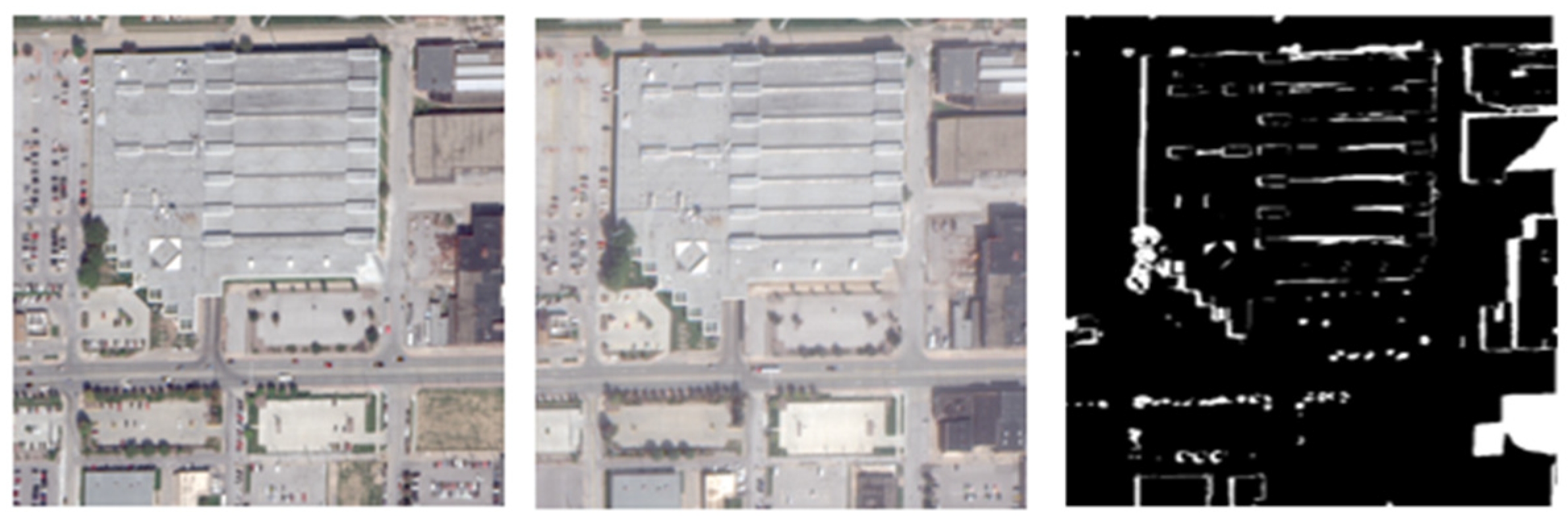
In this work, the baseline network Monster is used to predict the initial disparity for the left and right images, followed by a left–right consistency check [41] to generate an inaccurate ill-posed mask, representing the extent of ill-posed regions (Figure 3).
The formula for generating the inaccurate, ill-posed mask is as follows:
M ill   =     0 if   d gap     1 , 1 otherwise
d gap = | d L ( x ,   y ) d R   ( x + d L ( x ,   y ) ,   y ) |
Here, dgap denotes the disparity between corresponding pixels in the left and right views, while dL and dR represent the disparity maps of the left and right images, respectively.

3.3.2. Ill-Posed-Guided Adaptive Aware Geometry Fusion

The IAGF module takes as input the disparity D S i of the i-th iteration, the probability map Pro after cost calculation, and the left context feature F L   i of each iteration. Here, Pro represents confidence, indicating the relative disparity likelihood at each pixel and measuring the similarity between left and right features around D S i .
First, the probability distribution Pro is weighted by a disparity encoder, which applies a 1 × 1 convolution to perform a linear combination over C channels, yielding a single-channel weighted disparity map D W i . This map is concatenated with D S i along the channel dimension and subsequently passed through two 3 × 3 convolutional layers with ReLU activation, followed by a 1 × 1 convolution, to produce a single-channel matching feature map F fus i . By combining disparity and confidence cues, F fus i encodes the matching structure at the current stage.
Next, F fus i is concatenated with the left context feature F L   i , forming the local structural feature F local i , which captures reliable feature information in well-posed regions. In parallel, a self-attention module [42] is applied to F L   i to compute global spatial correlations, generating a correlation matrix A. By aggregating features across the global context, the global feature F glocal   i is obtained, enabling cross-region information propagation and enhancing feature completion in ill-posed regions.
Our work preserves local features in well-posed regions and global features in ill-posed regions. A linear relationship is established using the ill-posed region mask from the initial disparity to generate the aware feature FA [28]. FA contains global spatial context and structural information. The confidence-based local structural feature sufficiently supplements well-posed region features, while the global aggregated feature fills in missing information in ill-posed regions, effectively enhancing feature representation where data is unreliable.
F A i = A     ( concat ( DispEnc ( D S i ,   Pro i ) ,   F L   i ) )     M ill + (   A   ·   F L i )       I M ill
Here, M ill denotes the occlusion mask, D S i represents the disparity, I denotes the identity matrix, ⊙ indicates element-wise multiplication, and ⊗ denotes matrix–feature multiplication.
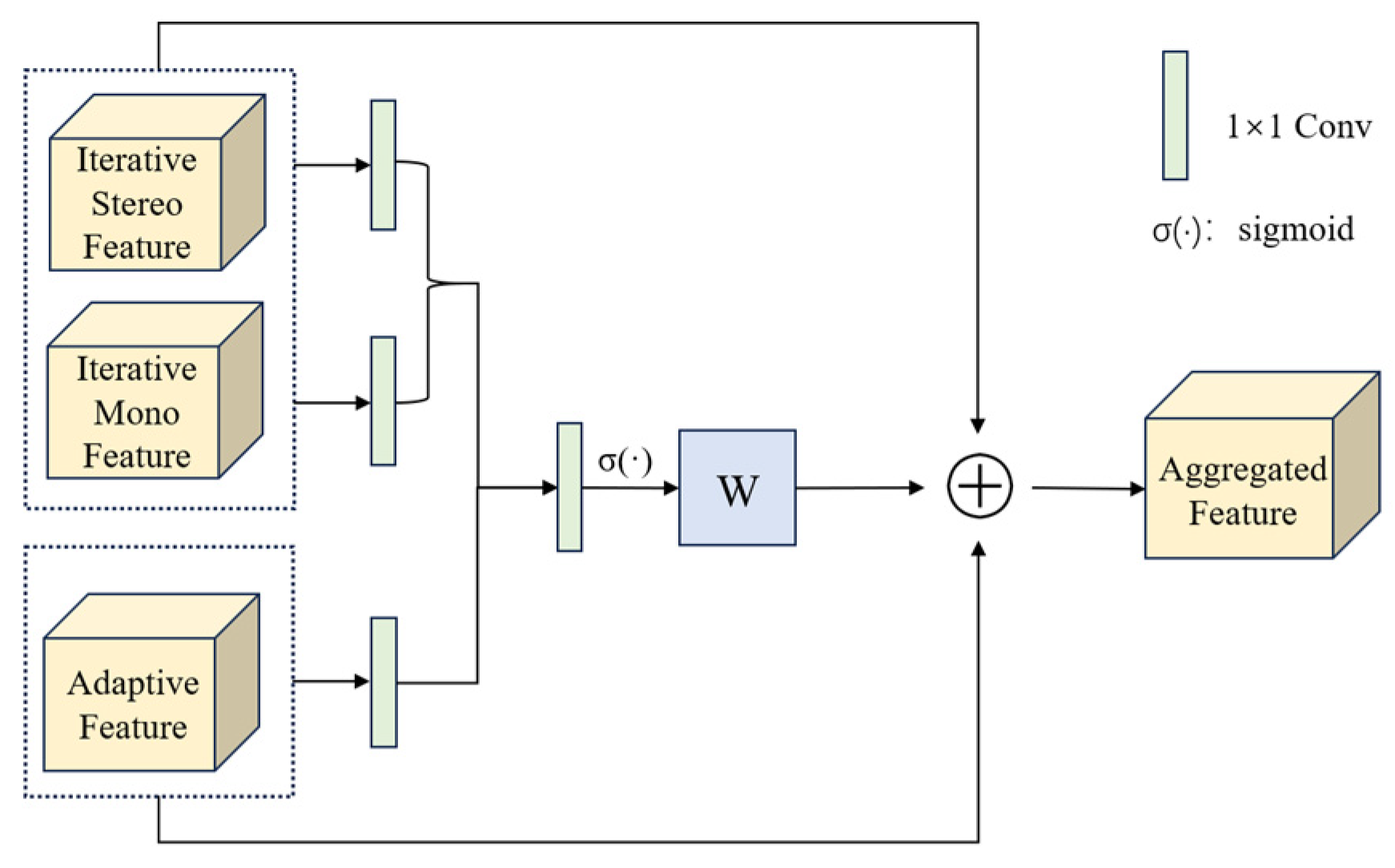
As shown in Figure 4, Adaptive Perceptual and Geometry Fusion (APGF) employs an adaptive weighting mechanism to effectively integrate the aware feature FA with the monocular and stereo geometric features (FS, FM). Specifically, a 1 × 1 convolutional projection layer first maps the aware and geometric features into a shared feature space, ensuring dimensional alignment and preserving key information. The projected features are then concatenated along the channel dimension and passed through a fusion layer to produce the fused representation. Finally, a convolutional attention weighting layer, followed by Sigmoid activation, generates a pixel-wise weight map W, which adaptively balances the contributions of aware and geometric features.
W = σ   ( Conv   ( [ Conv ( F A ) , Conv ( [ F S , F M ] ) ] ) )
Y = W     F A + ( 1 W )     [ F S , F M ]
Here, σ(·) is the Sigmoid function. A larger weight W indicates greater reliance on FA, while a smaller W favors the geometric features, enabling fine-grained, spatially adaptive feature fusion. This convolutional attention–based soft selection mechanism allows weights to vary across both spatial and channel dimensions, providing differentiated emphasis for regions affected by texture, boundaries, or illumination changes.
Finally, the fused feature Y, together with the residual features from the monocular and stereo branches ( F M j ,   F S j ), the geometric features ( G M j ,   G S j ), the disparities ( D M j ,   D S j ), and the context features ( c k ,   c r ,   c h ) are fed into the GRU. Through alternating refinement between SGA and MGR, the disparity is iteratively updated. Accordingly, the formulas for h m j and h S j in the Mutual Refinement part of Monster should be reformulated as follows:
h m j   =   ConvGRU h m j 1 , x S j , c k , c r , c h , Y
h S j = ConvGRU ( h S j 1 , x M j , c k , c r , c h , Y )
The core of this module lies in feature utilization, which integrates perceptual ill-posed features with geometric features derived from mono- and binocular networks. The perceptual ill-posed features provide prior understanding of scene structure and contextual awareness of object boundaries. Such features are crucial for making reasonable depth inferences in regions with missing textures or invalid matching cues. The geometric features, on the other hand, provide precise disparity-based geometric information and are highly reliable in regions with rich textures and favorable matching conditions. The joint integration of these two types of features effectively addresses the problem of performance degradation caused by the blind fusion of monocular information in baseline networks.

3.4. Data Augmentation and Train

3.4.1. Enhanced Mask Augmentation

In real stereo images, standard cost aggregation or correlation calculation often fails in unmatched regions. If the network is only exposed to matchable pixels during training, it becomes prone to erroneous reasoning. Inspired by traditional image enhancement strategies, we design regular occlusion augmentation and key-point mask augmentation. Our methods artificially create additional unmatched regions during training, allowing the model to encounter such situations in advance and learn to handle them correctly.
The regular occlusion augmentation randomly generates several rectangular regions in the right image of a stereo pair and replaces their pixel values with the global mean color, simulating partial information loss or occlusion. In our implementation, the occlusion blocks have sizes in the range [100, 200] pixels, and 1–5 blocks are applied randomly.
The key-point mask augmentation generates occlusion blocks centered on randomly selected key points, with a side length, forming a sparse dynamic mask M. Random rotations and translations, along with a global occlusion ratio constraint, are applied to ensure moderate and diverse coverage. The augmented image is obtained via element-wise multiplication:
I   =   I     M
Here, ⊙ denotes element-wise multiplication. Importantly, the erasing rate in this study is set to 1 enforcing the application of both augmentation strategies. Regular occlusion produces large, structured occlusions with mean-color replacement, simulating coarse information loss or object occlusion, while key-point mask augmentation generates small, diverse occlusion blocks with random perturbations, capturing fine-grained irregular occlusions, local structure variations, and partial information loss as often observed in natural scenes.

3.4.2. Loss Function

We adopt a hybrid loss function with dual-branch supervision [36]. The network consists of a monocular branch and a stereo branch, both with iterative structures that produce intermediate disparity maps at multiple stages. For each branch, the intermediate disparity maps at all stages are supervised using a weighted L1 loss. The overall loss function is defined as:
S moot h L 1 ( x )   =   0.5 x 2 , i f   x   <   1 , x     0.5 , o t h e r w i s e
L total = i = 0 N γ N i   Smooth L 1 d m   d gt + i = 0 N γ N i   Smooth L 1 d s     d gt  
Here, dgt denotes the ground-truth disparity, dm is the predicted disparity from the monocular branch, and ds is the predicted disparity from the stereo branch. The factor γ is an exponential weighting decay, set to γ = 0.9 in this work, such that the weights increase exponentially with iteration, emphasizing that later-stage disparity estimates are more confident [43].

4. Results

4.1. Experiment Setting

4.1.1. Datasets

US3D [44] is a large-scale remote sensing dataset for stereo matching and semantic understanding, originally introduced by IARPA in the 2019 Data Fusion Contest. In this work, we use the stereo semantic stereo matching subset. The dataset was captured by the WorldView-3 satellite between 2014 and 2016, covering the cities of Jacksonville and Omaha in the United States with high-resolution multi-view stereo imagery. The images are rigorously rectified and co-registered, forming 1024 × 1024 RGB stereo pairs with publicly available ground-truth disparity maps. The ground sampling distance of the imagery is approximately 30 cm, providing high spatial resolution.
In our study, we employ a corrected version of the US3D dataset (https://github.com/endu111/robust-satellite-image-stereo-matching, accessed on 13 July 2025.), which addresses errors in the original release and provides improved reliability for benchmarking stereo matching methods. The dataset contains a total of 4292 stereo pairs, with 2139 pairs from Jacksonville and 2153 pairs from Omaha. In our experiments, 1500 pairs from Jacksonville are used for training, 185 pairs for validation, and the remaining pairs for testing. All pairs from Omaha (2153 pairs) are used solely for evaluating the generalization performance of the model and are not included in the training process.

4.1.2. Evaluation Metrics

In this work, we adopt two widely used performance evaluation metrics for stereo matching: EPE (End-Point Error) and D1 (percentage of erroneous pixels). They are defined as follows:
EPE   =   1 N   i   =   1 N   | d pred ( i )     d gt ( i ) |
D 1 = 1 N   i = 1 N   | d pred ( i )     d gt ( i ) |   >   τ
Here, the End-Point Error (EPE) is defined as the mean absolute difference between the predicted disparity and the ground-truth disparity. Let d pred ( i ) and d gt ( i ) denote the predicted and ground-truth disparities of the i-th pixel, respectively, and N be the total number of valid pixels. Then, D1 represents the proportion of pixels for which the disparity prediction error exceeds a threshold τ, which is typically set to 3 pixels.

4.1.3. Implementation Details

We implement our network with PyTorch 1.13, and conduct all training on four NVIDIA RTX 3090 GPUs manufactured by NVIDIA Corporation, Santa Clara, CA, USA, each with 24 GB of memory. We adopt the AdamW optimizer [45], and, following the baseline setting [14], we apply gradient clipping within the range [−1, 1] to stabilize the training process. We employ a one-cycle learning rate schedule with an initial learning rate of 1 × 10⁻⁴ and train the model for 50,000 steps with a batch size of 8. We use the ViT backbone from DepthAnything V2 [34] for depth estimation in the monocular branch, freeze all its parameters during training, and set the disparity range to [−96, 96], consistent with prior works.

4.2. Results and Comparisons

In this subsection, we evaluate the proposed method on the US3D dataset and compare it with several representative stereo matching networks, including classical stereo matching networks such as PSMNet [12], CFNet [10], GWCNet [11], MSNet3D [46], Stereobase [47], IGEV [14], which represent different cost aggregation and feature extraction strategies, as well as stereo matching networks augmented with monocular depth information, namely DEFOMStereo [35], Monster [36]. To ensure a fair evaluation, we strictly follow the publicly available experimental setup, using images from the Jacksonville region for training and reserving images from the Omaha region, which are not included in training, for testing, thereby comprehensively assessing the model’s generalization capability in complex remote sensing scenarios.
Table 1 presents the quantitative evaluation results of different methods on the Omaha region. Using the well-posed and ill-posed region masks described above, the overall performance shows that our method achieves a D1 error of 5.38% and an EPE of 0.9582 across all regions (All), significantly outperforming the traditional stereo network IGEV as well as monocular-enhanced frameworks DEFOM and Monster, demonstrating superior overall accuracy and convergence.
Figure 5 illustrates a visual comparison of disparity maps produced by different methods on representative test images. It can be observed that, whether in structurally simple areas (e.g., flat roads and ground) or in complex regions (e.g., vegetation and buildings), our method generates disparity maps that are smoother and more continuous, whereas other methods often exhibit loss of details and matching artifacts, even when incorporating monocular information as in DEFOM and Monster.
These qualitative advantages are corroborated by the quantitative results presented in Table 2, which consistently demonstrate the superiority of our approach across key evaluation metrics.
Ours study systematically compares and evaluates methods addressing the three core challenges in cross-orbit satellite stereo matching: geometric differences, radiometric differences, and temporal variations. Geometric differences manifest in occluded regions, repetitive texture areas, and disparity discontinuities; radiometric differences are primarily evident in textureless regions; and temporal variations include both geometric transformations (such as building construction or demolition) and radiometric changes (such as seasonal vegetation variation).
To comprehensively assess the adaptability of different methods to complex remote sensing scenarios, six pairs of stereo images were carefully selected to cover representative challenging regions. Both visual results and quantitative metrics were analyzed in depth. As shown in the results above, conventional binocular stereo matching methods perform worse than the proposed approach. Therefore, we selected the currently competitive binocular method IGEV, the monocular-fusion networks DEFOM and Monster, and our proposed method for focused comparison and performance difference analysis.
In terms of radiometric differences, textureless regions pose significant challenges for stereo matching due to the lack of distinct texture features and edge information. As shown in Figure 6, in areas such as rooftops and bridges, the four methods exhibit noticeable performance differences: the other three methods either produce evident noise and ambiguity, show distortions along edges, or fail to preserve fine details. In contrast, the disparity map generated by the proposed method not only demonstrates the smoothest visual appearance but also effectively maintains structural integrity. Quantitative results in Table 3 further confirm this advantage. In the overall region of the OMA251_008_004 scene, the proposed method achieves a D1 error of 2.99, which is significantly lower than that of IGEV (7.22), DEFOM (6.24), and Monster (5.57). In the ill-posed regions, the proposed method achieves a D1 error of 18.85, representing a reduction of approximately 7–23 percentage points compared with the other methods, demonstrating its clear superiority in handling textureless regions.
In terms of geometric differences, disparity discontinuities and occluded regions pose significant challenges to convolutional neural networks due to their sharp depth transitions and large disparity gradients. Figure 7 presents a performance comparison of the four methods across typical scenes: IGEV exhibits noticeable boundary blurring and local distortions along building edges; DEFOM and Monster show considerable visual improvements over IGEV, yet still suffer from local noise interference in edge details and occluded regions. In contrast, the proposed method achieves smoother and more accurate disparity transitions along building boundaries and effectively infers and reconstructs occluded shadow regions.
The quantitative results in Table 4 further validate the superiority of the proposed method. In the most challenging OMA288_008_006 scene, the proposed approach achieves a D1 error of 31.05 in ill-posed regions, which is significantly lower than that of IGEV (42.30), DEFOM (41.37), and Monster (35.69), clearly demonstrating its strong adaptability and reconstruction capability in regions with sharp geometric variations.
Repetitive texture regions also represent a challenging case of geometric differences. Due to the presence of numerous visually similar features, accurate correspondence between the left and right images becomes difficult to establish. During disparity estimation, this ambiguity in determining unique correspondences often leads to estimation errors. Such textures are widely found in man-made structures and agricultural or forested areas. Figure 8 illustrates the performance of the proposed method in these scenarios. Compared with existing approaches, our model produces more accurate predictions in vegetation regions and maintains clearer and more complete building boundaries. Table 5 further provides quantitative evaluation results across different scenes, verifying the effectiveness of the proposed method. In handling repetitive pattern regions, different methods exhibit distinct characteristics. As shown in Figure 8, in urban and agricultural areas with abundant repetitive textures, IGEV suffers from severe mismatches; DEFOM yields relatively accurate predictions in vegetation regions but performs poorly in preserving building boundaries; Monster reduces error rates but tends to produce over-smoothed results in vegetated areas. In contrast, the proposed method preserves sharp and consistent building boundaries while achieving more accurate predictions in vegetation regions. The quantitative analysis in Table 5 shows that, in the ill-posed regions of the OMA391_025_019 scene, the proposed method achieves a D1 error of 23.34, nearly 10 percentage points lower than IGEV (32.99) and significantly outperforming the other comparative methods.
In terms of temporal variation differences, traditional stereo matching methods face significant challenges due to geometric changes and radiometric inconsistencies, which often lead to the loss of true correspondences. As shown in Figure 9, the building transformation and seasonal variation scenes clearly demonstrate the performance gaps among different methods. The IGEV method fails to provide valid disparity predictions, while the DEFOM method produces roughly reasonable results but introduces substantial noise. The Monster method performs better in structural preservation but generates many false details. In contrast, the proposed method maintains clear contours and yields the most accurate depth estimations. Quantitative results in Table 6 further verify its superiority: in the pathological regions of the OMA244_003_036 scene, the proposed method achieves a D1 error of 40.42, significantly lower than IGEV (56.66), DEFOM (45.64), and Monster (43.86), demonstrating excellent performance in handling temporal variation regions.
Through an in-depth analysis of the qualitative and quantitative performance of different methods across various challenging regions, it can be observed that the proposed method demonstrates particularly remarkable advantages in handling temporal variation areas. In contrast, the Monster network introduces significant noise due to its excessive reliance on information, and the DEFOM method shows limitations in structural preservation. Our method, however, effectively suppresses noise interference while maintaining strong structural integrity through a more balanced and efficient information utilization strategy.

5. Discussion

In one section, we conducted ablation experiments and Efficiency analysis.

5.1. Ablation Experiment

Ablation experiments were conducted on the proposed IAGF and EMA modules. We compared IAGF with the SRU scheme based on linear residual updates. To identify the optimal EMA mechanism, experiments were conducted based on the baseline model Monster. The end-point error (EPE) and D1 metrics were evaluated for the entire region (All), ill-posed regions, and well-posed regions.
As shown in Table 7, compared with the baseline model, incorporating EMA alone improves overall accuracy. Specifically, IGEV + EMA achieves notable improvements in both the overall and ill-posed regions, although the accuracy in well-posed regions slightly decreases, with the EPE increasing from 0.8357 to 0.8454. In contrast, Monster + EMA consistently reduces errors across all regions—overall, ill-posed, and well-posed—demonstrating stronger generalization. EMA is particularly effective in stereo matching networks that integrate monocular depth, especially in improving depth estimation accuracy in ill-posed regions. As illustrated in Figure 10, this module can generate more reasonable predictions in areas originally lacking matches or depth responses, although improvements at object boundaries and structural contours remain relatively limited.
To identify the optimal EMA mechanism, experiments were conducted based on the baseline model Monster. As shown in Table 8, EMA led to improvements in accuracy, demonstrating the effectiveness of the proposed module. With all other parameters kept constant, increasing the number of occlusion blocks to [1, 5] further reduced the D1 error in ill-posed regions by 0.51% (from 23.53% to 23.02%). This indicates that increasing the density of random occlusions helps enhance the model’s generalization ability. When the occlusion block size was enlarged to [100, 200], the D1 error in ill-posed regions dropped more significantly, from 23.02% to 22.31%, a reduction of 0.71%. This suggests that larger occlusion regions more effectively force the model to learn long-range contextual information and global structure rather than relying on local textures, resulting in better performance in large ill-posed regions.
Compared with the marginal gains from adjusting the number and size of occlusion blocks, setting the erasing rate to 1 achieved the largest reduction in D1 error in ill-posed regions, decreasing by 1.2% (from 22.31% to 22.04%). More importantly, it was the only strategy that also significantly improved overall performance (overall D1 decreased from 5.49% to 5.47%). These results indicate that sustained high-difficulty training most effectively forces the model to move beyond reliance on local features and learn global reasoning capabilities, making the erasing rate a more critical factor for accuracy improvement than occlusion geometry parameters.
Integrating monocular depth into the Monster network improves disparity estimation in ill-posed regions, but accuracy in some originally well-matched areas may decrease. Since the network is fundamentally based on iterative residual updates, the simplest way to address this issue is the Selective Residual Update (SRU), which linearly updates the disparity residual Δd according to an ill-posed detection mask. Using the mask, Mill derived from the initial disparity, the residual from the normal update branch is applied in well-posed regions, while the residual incorporating monocular depth predictions is applied in ill-posed regions, thus avoiding the accumulation of erroneous gradients.
We compare the proposed IAGF module with the SRU scheme across three networks: Monster and DEFOM. As shown in Table 7, for the Monster model, applying IAGF (Monster + IAGF) reduces the EPE in ill-posed regions from 2.4074 to 2.2202, achieving a 7.77% improvement; with SRU, the EPE decreases to 2.2352, a 7.15% improvement. For the DEFOM model, integrating IAGF reduces the overall EPE from 0.9950 to 0.9687 (2.7% improvement), while SRU reduces it to 0.9781. These results demonstrate that IAGF outperforms SRU and yields clearer and more complete structural contours, as shown in Figure 10.
Further generalization tests indicate that incorporating IAGF consistently improves accuracy across overall, ill-posed, and well-posed regions for both Monster and DEFOM. Notably, in scenarios involving occlusions and geometric transformations, IAGF more effectively preserves depth consistency and structural integrity, while mitigating redundant noise introduced by monocular fusion, thereby demonstrating stronger robustness and generalization in complex scenes.
The actual contribution of the two modules to the network can be clearly observed from the experiments. Taking IGEV and Monster as examples, the mask augmentation mechanism provides a consistent and positive performance improvement for both models, with reductions in EPE and D1-all. However, the magnitude of this improvement (EPE 0.01–0.04, D1-all 0.15–0.21%) is far smaller than the gains brought by the IAGF module. For instance, in the Monster model, incorporating EMA reduces the EPE from 0.9696 to 0.9685, whereas adding IAGF further decreases the EPE to 0.9611.

5.2. Efficiency Analysis

To evaluate the practicality of the proposed method, this section compares the efficiency performance of IAASNet with baseline methods under a unified software and hardware environment, using input images with a fixed resolution of 1024 × 1024.
As shown in Table 9, compared with the baseline Monster method, the inference time per image increases from 0.65 s to 1.42 s for the proposed method, with a total model parameter count of 388.89 M. Although Monster has slightly fewer parameters, our method achieves significant improvements in accuracy and generalization with only a marginal increase of 0.2 M parameters. In our network, the EMA enhancement mechanism does not introduce additional parameters. Results demonstrate that the designed IAGF module is lightweight and effectively improves the handling of ill-posed regions in stereo matching with almost no added computational burden.
Our study focuses on optimizing accuracy and generalization. The proposed method reduces EPE from 5.50 to 5.38, a relative improvement of 2.18%, and shows superior generalization performance, indicating that the additional inference cost is acceptable. Notably, when the number of iterations is reduced to 16, the inference time drops to 0.72 s while maintaining an excellent D1-all score of 0.9593, comparable to the 32-iteration version. Further reducing the iterations to 8 allows the model to maintain an EPE of 5.42 with an inference time of 0.66 s, matching the baseline in time consumption while achieving higher accuracy.
Through careful module design, the proposed method achieves significant improvements in matching accuracy and generalization with minimal parameter growth and controllable time overhead.

6. Conclusions

The core of remote sensing stereo matching lies in accurately establishing correspondences between the left and right views to estimate disparities. However, due to factors such as multi-temporal acquisition, multi-sensor heterogeneity, and cross-orbit imaging, remote sensing images frequently exhibit textureless regions, occlusions, structural deformations, and radiometric variations. Specifically, flat rooftops, roads, severe occlusions by high-rise buildings or terrain, and seasonal vegetation changes pose substantial challenges to stereo matching.
In this work, we propose a perceptually ill-posed stereo matching framework, which incorporates Enhanced Mask Augmentation (EMA) and the Ill-posed-guided Adaptive Aware Geometry Fusion (IAGF) module. EMA introduces artificial unmatched regions during training, causing cost-volume features in these regions to produce low-confidence responses or rely on neighborhood information for inference. This significantly improves the model’s generalization and robustness across diverse scenarios. Ablation studies indicate that EMA contributes positively to overall disparity accuracy, particularly in ill-posed regions, though its effect is less pronounced than that of IAGF. When combined with monocular depth information, EMA achieves even higher precision in ill-posed regions, as it forces the model to learn to infer disparities in unmatched regions and complements this with monocular depth cues.
To mitigate the potential noise and performance degradation caused by naive monocular fusion, we design the IAGF module, which adaptively aggregates local features from well-posed regions and global features from ill-posed regions. The resulting aware features are fused with both monocular and stereo geometric features in a fine-grained, stable, and efficient manner. Experimental results demonstrate that integrating IAGF improves accuracy across overall, ill-posed, and well-posed regions, while also exhibiting strong generalization, confirming its effectiveness in suppressing redundant information, enhancing structural awareness, and improving feature fusion.
Overall, our network effectively alleviates challenges in remote sensing stereo matching, achieving superior performance across multiple metrics on the US3D dataset, especially in regions affected by occlusion and structural variations.
The limitations of the current approach lie in its relatively complex network architecture and high computational resource consumption, as well as the room for improvement in the efficiency of monocular depth utilization. In the future, we aim to focus on lightweight backbone network designs and explore techniques such as model quantization and distillation to enhance the practicality and deployment efficiency of the method. Additionally, we will investigate more efficient mechanisms for monocular depth utilization to leverage structural priors more accurately while suppressing noise. Furthermore, we plan to construct a cross-track remote sensing stereo dataset that covers a wider range of temporal phases and more complex land-cover changes, providing a more robust data foundation for model training and evaluation.

Author Contributions

Conceptualization, J.H. and H.S.; methodology, J.H. and H.S.; software, J.H. and H.S.; validation, J.H. and H.S.; formal analysis, J.H.; investigation, J.H.; resources, H.S. and T.W.; data curation, J.H.; writing—original draft preparation, J.H.; writing—review and editing, J.H.; visualization, J.H.; supervision, J.H. and H.S.; project administration, J.H. and H.S.; funding acquisition, T.W. All authors have read and agreed to the published version of the manuscript.

Funding

This research received no external funding.

Data Availability Statement

The Urban Semantic 3D dataset (US3D) from Data Fusion Contest 2019(DFC2019) can be found at https://ieee-dataport.org/open-access/data-fusion-contest-2019-dfc2019 (accessed on 21 April 2023). Subsequently, the corrected US3D dataset can be found at https://github.com/endu111/robust-satellite-image-stereo-matching (accessed on 3 September 2025).

Acknowledgments

The authors would like to express their sincere gratitude to IARPA and the Johns Hopkins University Applied Physics Laboratory for generously providing the high-quality US3D dataset. The authors also wish to especially thank the second author, Haoxuan Sun, for providing the corrected version of the US3D dataset.

Conflicts of Interest

The authors declare no conflicts of interest.

References

  1. Stucker, C.; Schindler, K. ResDepth: A Deep Residual Prior for 3D Reconstruction from High-Resolution Satellite Images. ISPRS J. Photogramm. Remote Sens. 2022, 183, 560–580. [Google Scholar] [CrossRef]
  2. Ji, S.; Liu, J.; Lu, M. CNN-Based Dense Image Matching for Aerial Remote Sensing Images. Photogramm. Eng. Remote Sens. 2019, 85, 415–424. [Google Scholar] [CrossRef]
  3. Jiang, S.; Jiang, W.; Wang, L. Unmanned Aerial Vehicle-Based Photogrammetric 3D Mapping: A Survey of Techniques, Applications, and Challenges. IEEE Geosci. Remote Sens. Mag. 2022, 10, 135–171. [Google Scholar] [CrossRef]
  4. He, S.; Li, S.; Jiang, S.; Jiang, W. HMSM-Net: Hierarchical Multi-Scale Matching Network for Disparity Estimation of High-Resolution Satellite Stereo Images. ISPRS J. Photogramm. Remote Sens. 2022, 188, 314–330. [Google Scholar] [CrossRef]
  5. He, S.; Zhou, R.; Li, S.; Jiang, S.; Jiang, W. Disparity Estimation of High-Resolution Remote Sensing Images with Dual-Scale Matching Network. Remote Sens. 2021, 13, 5050. [Google Scholar] [CrossRef]
  6. Khamis, S.; Fanello, S.; Rhemann, C.; Kowdle, A.; Valentin, J.; Izadi, S. StereoNet: Guided Hierarchical Refinement for Real-Time Edge-Aware Depth Prediction. In Proceedings of the European Conference on Computer Vision (ECCV), Munich, Germany, 8–14 September 2018; pp. 573–590. [Google Scholar]
  7. Cao, Y.; Xu, J.; Lin, S.; Wei, F.; Hu, H. GCNet: Non-Local Networks Meet Squeeze-Excitation Networks and Beyond. In Proceedings of the 2019 IEEE/CVF International Conference on Computer Vision Workshop (ICCVW), Seoul, Republic of Korea, 27–28 October 2019; pp. 1971–1980. [Google Scholar]
  8. Gu, X.; Fan, Z.; Zhu, S.; Dai, Z.; Tan, F.; Tan, P. Cascade Cost Volume for High-Resolution Multi-View Stereo and Stereo Matching. In Proceedings of the 2020 IEEE/CVF Conference on Computer Vision and Pattern Recognition (CVPR), Seattle, WA, USA, 13–19 June 2020; pp. 2492–2501. [Google Scholar]
  9. Wang, T.; Ma, C.; Su, H.; Wang, W. CSPN: Multi-Scale Cascade Spatial Pyramid Network for Object Detection. In Proceedings of the ICASSP 2021—2021 IEEE International Conference on Acoustics, Speech and Signal Processing (ICASSP), Toronto, ON, Canada, 6–11 June 2021; pp. 1490–1494. [Google Scholar]
  10. Shen, Z.; Dai, Y.; Rao, Z. CFNet: Cascade and Fused Cost Volume for Robust Stereo Matching. In Proceedings of the 2021 IEEE/CVF Conference on Computer Vision and Pattern Recognition (CVPR), Nashville, TN, USA, 20–25 June 2021; pp. 13906–13915. [Google Scholar]
  11. Guo, X.; Yang, K.; Yang, W.; Wang, X.; Li, H. Group-Wise Correlation Stereo Network. In Proceedings of the 2019 IEEE/CVF Conference on Computer Vision and Pattern Recognition (CVPR), Long Beach, CA, USA, 15–20 June 2019; pp. 3268–3277. [Google Scholar]
  12. Chang, J.-R.; Chen, Y.-S. Pyramid Stereo Matching Network. In Proceedings of the 2018 IEEE/CVF Conference on Computer Vision and Pattern Recognition, Salt Lake City, UT, USA, 18–23 June 2018; pp. 5410–5418. [Google Scholar]
  13. Zhang, F.; Prisacariu, V.; Yang, R.; Torr, P.H.S. GA-Net: Guided Aggregation Net for End-To-End Stereo Matching. In Proceedings of the 2019 IEEE/CVF Conference on Computer Vision and Pattern Recognition (CVPR), Long Beach, CA, USA, 15–20 June 2019; pp. 185–194. [Google Scholar]
  14. Xu, G.; Wang, X.; Ding, X.; Yang, X. Iterative Geometry Encoding Volume for Stereo Matching. In Proceedings of the 2023 IEEE/CVF Conference on Computer Vision and Pattern Recognition (CVPR), Vancouver, BC, Canada, 17–24 June 2023; pp. 21919–21928. [Google Scholar]
  15. Jeong, W.; Park, S.-Y. UGC-Net: Uncertainty-Guided Cost Volume Optimization with Contextual Features for Satellite Stereo Matching. Remote Sens. 2025, 17, 1772. [Google Scholar] [CrossRef]
  16. Kim, J.; Cho, S.; Chung, M.; Kim, Y. Improving Disparity Consistency with Self-Refined Cost Volumes for Deep Learning-Based Satellite Stereo Matching. IEEE J. Sel. Top. Appl. Earth Obs. Remote Sens. 2025, 18, 9262–9278. [Google Scholar] [CrossRef]
  17. Cheng, J.; Yin, W.; Wang, K.; Chen, X.; Wang, S.; Yang, X. Adaptive Fusion of Single-View and Multi-View Depth for Autonomous Driving. In Proceedings of the 2024 IEEE/CVF Conference on Computer Vision and Pattern Recognition (CVPR), Seattle, WA, USA, 16–22 June 2024; pp. 10138–10147. [Google Scholar]
  18. Li, K.; Wang, L.; Zhang, Y.; Xue, K.; Zhou, S.; Guo, Y. LoS: Local Structure-Guided Stereo Matching. In Proceedings of the 2024 IEEE/CVF Conference on Computer Vision and Pattern Recognition (CVPR), Seattle, WA, USA, 16–22 June 2024; pp. 19746–19756. [Google Scholar]
  19. Yang, G.; Zhao, H.; Shi, J.; Deng, Z.; Jia, J. SegStereo: Exploiting Semantic Information for Disparity Estimation. In Computer Vision—ECCV 2018; Ferrari, V., Hebert, M., Sminchisescu, C., Weiss, Y., Eds.; Lecture Notes in Computer Science; Springer International Publishing: Cham, Switzerland, 2018; Volume 11211, pp. 660–676. ISBN 978-3-030-01233-5. [Google Scholar]
  20. Guo, W.; Li, Z.; Yang, Y.; Wang, Z.; Taylor, R.H.; Unberath, M.; Yuille, A.; Li, Y. Context-Enhanced Stereo Transformer. In Proceedings of the Computer Vision—ECCV 2022; Avidan, S., Brostow, G., Cissé, M., Farinella, G.M., Hassner, T., Eds.; Springer Nature: Cham, Switzerland, 2022; pp. 263–279. [Google Scholar]
  21. EdgeStereo: An Effective Multi-Task Learning Network for Stereo Matching and Edge Detection|International Journal of Computer Vision. Available online: https://link.springer.com/article/10.1007/s11263-019-01287-w (accessed on 1 September 2025).
  22. Liao, P.; Zhang, X.; Chen, G.; Wang, T.; Li, X.; Yang, H.; Zhou, W.; He, C.; Wang, Q. S2Net: A Multitask Learning Network for Semantic Stereo of Satellite Image Pairs. IEEE Trans. Geosci. Remote Sens. 2024, 62, 1–13. [Google Scholar] [CrossRef]
  23. Yang, Q.; Chen, G.; Tan, X.; Wang, T.; Wang, J.; Zhang, X. S3Net: Innovating Stereo Matching and Semantic Segmentation with a Single-Branch Semantic Stereo Network in Satellite Epipolar Imagery. In Proceedings of the IGARSS 2024—2024 IEEE International Geoscience and Remote Sensing Symposium, Athens, Greece, 7–12 July 2024; pp. 8737–8740. [Google Scholar]
  24. Wu, Z.; Wu, X.; Zhang, X.; Wang, S.; Ju, L. Semantic Stereo Matching with Pyramid Cost Volumes. In Proceedings of the 2019 IEEE/CVF International Conference on Computer Vision (ICCV), Seoul, Republic of Korea, 27 October–2 November 2019; pp. 7484–7493. [Google Scholar]
  25. Heo, Y.S.; Lee, K.M.; Lee, S.U. Joint Depth Map and Color Consistency Estimation for Stereo Images with Different Illuminations and Cameras. IEEE Trans. Pattern Anal. Mach. Intell. 2013, 35, 1094–1106. [Google Scholar] [CrossRef] [PubMed]
  26. Liang, X.; Jung, C. Deep Cross Spectral Stereo Matching Using Multi-Spectral Image Fusion. IEEE Robot. Autom. Lett. 2022, 7, 5373–5380. [Google Scholar] [CrossRef]
  27. Li, Z.; Liu, X.; Drenkow, N.; Ding, A.; Creighton, F.X.; Taylor, R.H.; Unberath, M. Revisiting Stereo Depth Estimation from a Sequence-to-Sequence Perspective with Transformers. In Proceedings of the 2021 IEEE/CVF International Conference on Computer Vision (ICCV), Montreal, QC, Canada, 10–17 October 2021; pp. 6197–6206. [Google Scholar]
  28. Liu, Z.; Li, Y.; Okutomi, M. Global Occlusion-Aware Transformer for Robust Stereo Matching. In Proceedings of the 2024 IEEE/CVF Winter Conference on Applications of Computer Vision (WACV), Waikoloa, HI, USA, 3–8 January 2024; pp. 3523–3532. [Google Scholar]
  29. Learning Stereo from Single Images|SpringerLink. Available online: https://link.springer.com/chapter/10.1007/978-3-030-58452-8_42 (accessed on 1 September 2025).
  30. Muresan, M.P.; Raul, M.; Nedevschi, S.; Danescu, R. Stereo and Mono Depth Estimation Fusion for an Improved and Fault Tolerant 3D Reconstruction. In Proceedings of the 2021 IEEE 17th International Conference on Intelligent Computer Communication and Processing (ICCP), Cluj-Napoca, Romania, 28–30 October 2021; pp. 233–240. [Google Scholar]
  31. Zhang, C.; Meng, G.; Su, B.; Xiang, S.; Pan, C. Monocular Contextual Constraint for Stereo Matching with Adaptive Weights Assignment. Image Vis. Comput. 2022, 121, 104424. [Google Scholar] [CrossRef]
  32. Jiang, J.; Liao, X.; Yang, F.; Cheung, K.; Wang, X.; Zhao, Y. Leveraging Monocular Depth and Feature Fusion for Generalized Stereo Matching. In Proceedings of the 2025 IEEE 6th International Seminar on Artificial Intelligence, Networking and Information Technology (AINIT), Shenzhen, China, 11–13 April 2025; pp. 1–5. [Google Scholar]
  33. Wen, B.; Trepte, M.; Aribido, J.; Kautz, J.; Gallo, O.; Birchfield, S. FoundationStereo: Zero-Shot Stereo Matching. In Proceedings of the Computer Vision and Pattern Recognition Conference, Nashville, TN, USA, 10–17 June 2025; pp. 5249–5260. [Google Scholar]
  34. Yang, L.; Kang, B.; Huang, Z.; Zhao, Z.; Xu, X.; Feng, J.; Zhao, H. Depth Anything V2. Adv. Neural Inf. Process. Syst. 2024, 37, 21875–21911. [Google Scholar]
  35. Jiang, H.; Lou, Z.; Ding, L.; Xu, R.; Tan, M.; Jiang, W.; Huang, R. DEFOM-Stereo: Depth Foundation Model Based Stereo Matching. In Proceedings of the Computer Vision and Pattern Recognition Conference, Nashville, TN, USA, 10–17 June 2025; pp. 21857–21867. [Google Scholar]
  36. Cheng, J.; Liu, L.; Xu, G.; Wang, X.; Zhang, Z.; Deng, Y.; Zang, J.; Chen, Y.; Cai, Z.; Yang, X. MonSter: Marry Monodepth to Stereo Unleashes Power. In Proceedings of the Computer Vision and Pattern Recognition Conference, Nashville, TN, USA, 10–17 June 2025; pp. 6273–6282. [Google Scholar]
  37. Oquab, M.; Darcet, T.; Moutakanni, T.; Vo, H.; Szafraniec, M.; Khalidov, V.; Fernandez, P.; Haziza, D.; Massa, F.; El-Nouby, A.; et al. DINOv2: Learning Robust Visual Features without Supervision. arXiv 2024, arXiv:2304.07193. [Google Scholar] [CrossRef]
  38. Ranftl, R.; Bochkovskiy, A.; Koltun, V. Vision Transformers for Dense Prediction. In Proceedings of the 2021 IEEE/CVF International Conference on Computer Vision (ICCV), Montreal, QC, Canada, 10–17 October 2021; pp. 12179–12188. [Google Scholar]
  39. Hirschmuller, H.; Scharstein, D. Evaluation of Stereo Matching Costs on Images with Radiometric Differences. IEEE Trans. Pattern Anal. Mach. Intell. 2009, 31, 1582–1599. [Google Scholar] [CrossRef] [PubMed]
  40. Zitnick, C.L.; Kanade, T. A Cooperative Algorithm for Stereo Matching and Occlusion Detection. IEEE Trans. Pattern Anal. Mach. Intell. 2000, 22, 675–684. [Google Scholar] [CrossRef]
  41. Kanade, T.; Okutomi, M. A Stereo Matching Algorithm with an Adaptive Window: Theory and Experiment. IEEE Trans. Pattern Anal. Mach. Intell. 1994, 16, 920–932. [Google Scholar] [CrossRef]
  42. Jiang, S.; Campbell, D.; Lu, Y.; Li, H.; Hartley, R. Learning To Estimate Hidden Motions with Global Motion Aggregation. In Proceedings of the 2021 IEEE/CVF International Conference on Computer Vision (ICCV), Montreal, QC, Canada, 10–17 October 2021; pp. 9772–9781. [Google Scholar]
  43. Lipson, L.; Teed, Z.; Deng, J. RAFT-Stereo: Multilevel Recurrent Field Transforms for Stereo Matching. In Proceedings of the 2021 International Conference on 3D Vision (3DV), London, UK, 1–3 December 2021; pp. 218–227. [Google Scholar]
  44. Bosch, M.; Foster, K.; Christie, G.; Wang, S.; Hager, G.D.; Brown, M. Semantic Stereo for Incidental Satellite Images. In Proceedings of the 2019 IEEE Winter Conference on Applications of Computer Vision (WACV), Waikoloa, HI, USA, 7–11 January 2019; pp. 1524–1532. [Google Scholar]
  45. Loshchilov, I.; Hutter, F. Decoupled Weight Decay Regularization. arXiv 2019, arXiv:1711.05101. [Google Scholar] [CrossRef]
  46. WACV 2022 Open Access Repository. Available online: https://openaccess.thecvf.com/content/WACV2022/html/Shamsafar_MobileStereoNet_Towards_Lightweight_Deep_Networks_for_Stereo_Matching_WACV_2022_paper.html (accessed on 1 September 2025).
  47. Guo, X.; Zhang, C.; Lu, J.; Duan, Y.; Wang, Y.; Yang, T.; Zhu, Z.; Chen, L. OpenStereo: A Comprehensive Benchmark for Stereo Matching and Strong Baseline. arXiv 2024, arXiv:2312.00343. [Google Scholar] [CrossRef]
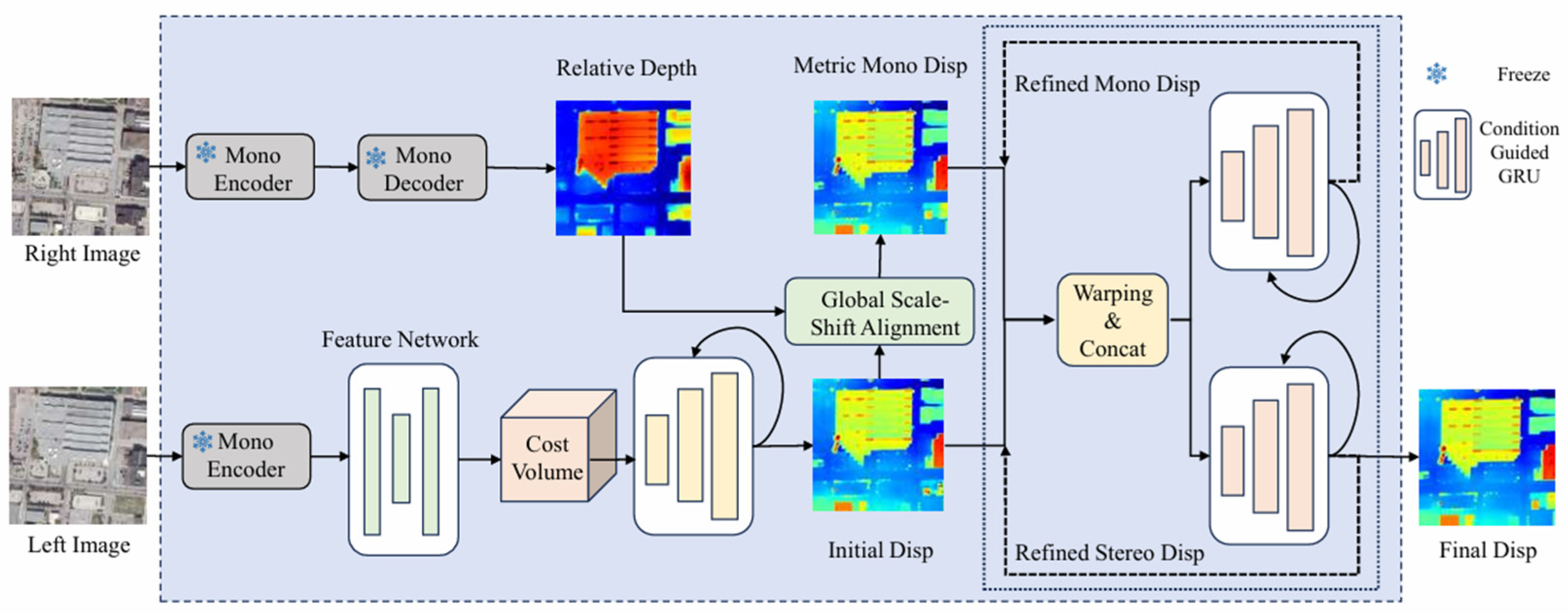
Figure 1. The overall architecture of Monster. Monster consists of a monocular depth branch, a stereo matching branch, and a mutual refinement module, which collaboratively perform coarse-to-fine iterative corrections with mono–stereo guidance to generate the final disparity.
Remotesensing 17 03528 g001
Figure 2. The overall architecture of the proposed model. IAASNet consists of the Monster monocular–stereo matching network highlighted in the blue-shaded area and the IAGF module highlighted in the orange-shaded area. Through IAGF, aware features from well-posed and ill-posed regions are extracted and iteratively optimized together with monocular and stereo geometric features within a refinement GRU, generating the final disparity.
Remotesensing 17 03528 g002
Figure 3. Left images, right images, and the predicted ill-posed mask from the US3D dataset.
Remotesensing 17 03528 g003
Figure 4. Adaptive Perceptual and Geometry Fusion (APGF) Module.
Remotesensing 17 03528 g004
Figure 5. The qualitative comparison of disparity maps produced by different methods. For clarity, selected regions of the disparity maps have been cropped and enlarged. From left to right: left image, PSMNet [12], CFNet [10], GWCNet [11], MSNet3D [46], Stereobase [47], IGEV [14], DEFOMStereo [35], Monster [36], IAASNet (ours), and the ground truth.
Remotesensing 17 03528 g005
Figure 6. The qualitative comparison of disparity maps across textureless regions produced by various methods. For clarity, selected regions of the disparity maps have been cropped and enlarged. From left to right: left image, right image, IGEV [14], DEFOM [35], Monster [36], IAASNet (ours), ground truth, and the ill-posed mask of the initial disparity. The images are arranged from top to bottom as follows: OMA251_008_004, OMA247_035_001.
Remotesensing 17 03528 g006
Figure 7. The qualitative comparison of disparity maps across disparity discontinuity and occlusion regions. produced by various methods. For clarity, selected regions of the disparity maps have been cropped and enlarged. From left to right: left image, right image, IGEV [14], DEFOM [35], Monster [36], IAASNet (ours), ground truth, and the ill-posed mask of the initial disparity. The images are arranged from top to bottom as follows: OMA212_008_006, OMA225_027_021, OMA281_006_027, OMA288_008_006.
Remotesensing 17 03528 g007
Figure 8. The qualitative comparison of disparity maps across repetitive pattern regions produced by various methods. For clarity, selected regions of the disparity maps have been cropped and enlarged. From left to right: left image, right image, IGEV [14], DEFOM [35], Monster [36], IAASNet (ours), ground truth, and the ill-posed mask of the initial disparity. The images are arranged from top to bottom as follows: OMA132_002_034, OMA391_025_019.
Remotesensing 17 03528 g008
Figure 9. The qualitative comparison of disparity maps across temporal variation regions. produced by various methods. For clarity, selected regions of the disparity maps have been cropped and enlarged. From left to right: left image, right image, IGEV [14], DEFOM [35], Monster [36], IAASNet (ours), ground truth, and the ill-posed mask of the initial disparity. The images are arranged from top to bottom as follows: OMA244_003_036, OMA172_027_019.
Remotesensing 17 03528 g009
Figure 10. Visualization of experiments based on the US3D dataset. For clarity, selected regions of the disparity maps have been cropped and enlarged. From left to right, the results correspond to the methods listed in Table 7 from top to bottom, followed by ours, the ground truth, and the ill-posed mask.
Remotesensing 17 03528 g010
Table 1. The quantitative comparison of various methods on the Omaha city data from the US3D dataset. We adopt the EPE-All results from the original papers. The division between well-posed and ill-posed regions follows the masks described above. Our model achieves the highest accuracy across all regions, including the overall, well-posed, and ill-posed areas. Red Bold: Best. Bold: Second.
ClassAllWell-PosedIll-Posed
ModelD1epeD1epeD1epe
PSMnet [12]6.611.13034.590.971727.512.7923
CFNet [10]6.151.04654.180.895326.172.6048
GWCNet [11]6.221.06784.270.915526.182.6500
MSNet3D [46]6.561.10824.560.954927.062.7243
Stereobase [47]6.081.02684.150.876125.822.5884
IGEV [14]5.600.97543.750.835724.292.4215
DEFOStereo [35]5.590.99503.850.861223.242.3639
Monster [36]5.500.96963.860.845424.102.4074
IAASNet (ours)5.380.95823.750.835521.762.2199
Table 2. The quantitative evaluation of the above images across different models. Red Bold: Best. Bold: Second.
ModelMetricsPSMnetCFNetGWCMSNet
3D
Stereo
Base
IGEVDEFOMMonsterIAAS
Net
OMA
132_042_026
D16.596.266.036.046.147.628.116.085.72
epe1.13681.05411.03111.03580.97971.42651.14810.97010.9444
OMA
212_007_041
D13.701.720.522.580.401.321.990.690.58
epe0.94410.81990.83350.83890.63861.40620.71620.63250.6234
OMA
315_036_030
D18.248.277.767.837.517.8011.416.436.18
epe1.11741.08371.03611.13361.00311.45511.52780.97230.9683
OMA
383_001_027
D12.492.042.695.221.927.181.431.501.15
epe0.79290.73160.79280.94510.70411.80480.68140.74080.6581
Table 3. The quantitative evaluation of stereo IGEV [14], Stereobase [47], and monocular-enhanced networks DEFOM [35] and IAASNet (ours) across overall regions and ill-posed regions of the textureless areas. Red Bold: Best. Bold: Second.
ModelClassMetricsIGEVDEFOMMonsterIAASNet
OMA
251_008_004
AllD17.226.245.572.99
epe1.18771.17270.98560.8074
illD141.4025.7126.3618.85
epe4.16192.66312.51432.1047
OMA
247_035_001
AllD111.423.972.312.30
epe2.02440.78830.78150.7719
illD136.7716.7014.3013.63
epe2.75841.60081.59811.5594
Table 4. The quantitative evaluation of stereo IGEV [14], Stereobase [47], and monocular-enhanced networks DEFOM [35] and IAASNet (ours) across overall regions and ill-posed regions of the disparity discontinuity and occlusion regions. Red Bold: Best. Bold: Second.
ModelClassMetricsIGEVDEFOMMonsterIAASNet
OMA
212_008_006
AllD12.471.491.231.06
epe0.73090.67310.64400.6469
illD113.1912.0610.289.18
epe1.35361.46201.16511.2591
OMA
225_027_021
AllD13.222.962.642.41
epe1.46750.76720.68730.7110
illD118.8518.9018.7717.52
epe1.78841.76411.76891.7221
OMA
281_006_027
AllD15.261.801.881.68
epe1.51890.66750.68800.6365
illD125.5316.5818.6916.23
epe2.47921.96562.19951.9362
OMA
288_008_006
AllD116.3615.3312.7511.72
epe1.96822.03841.75781.6750
illD142.3041.3735.6931.05
epe4.15753.87763.58243.2646
Table 5. The quantitative evaluation of stereo IGEV [14], Stereobase [47], and monocular-enhanced networks DEFOM [35] and IAASNet (ours) across overall regions and ill-posed regions of the repetitive pattern regions. Red Bold: Best. Bold: Second.
ModelClassMetricsIGEVDEFOMMonsterIAASNet
OMA
132_002_034
AllD134.838.238.257.94
epe2.88861.10811.13411.0991
illD148.0821.8520.9320.40
epe3.40582.01101.98441.9365
OMA
391_025_019
AllD112.5011.4312.0410.88
epe1.56401.44131.44111.3879
illD132.9928.7128.1423.34
epe3.20792.85412.69492.4983
Table 6. The quantitative evaluation of stereo IGEV [14], Stereobase [47], and monocular-enhanced networks DEFOM [35] and IAASNet (ours) across overall regions and ill-posed regions of the temporal variation regions. Red Bold: Best. Bold: Second.
ModelClassMetricsIGEVDEFOMMonsterIAASNet
OMA
244_003_036
AllD110.729.139.048.21
epe1.64741.34141.30231.2453
illD156.6645.6443.8640.42
epe6.02674.51894.09733.7137
OMA
172_027_019
AllD113.306.076.596.03
epe1.94380.97371.00430.9708
illD143.9122.4323.0020.39
epe3.42192.10472.13812.0072
Table 7. Experimental results of our network on the US3D dataset. Red Bold: Best. Bold: Second.
Class AllWell-PosedIll-Posed
ModelEMAIAGFD1epeD1epeD1epe
IGEV 5.600.97533.790.835724.292.4215
IGEV + EMA 5.560.97133.860.845424.102.4074
DEFOM 5.590.99503.850.861223.242.3639
DEFOM + IAGF 5.470.96873.720.832723.132.3523
Monster 5.500.96963.860.845424.102.4074
Monster + EMA 5.470.96853.820.844222.042.2517
Monster + SRU 5.460.96743.840.839121.902.2352
Monster + IAGF 5.440.96113.820.837821.772.2202
Table 8. Experimental results to identify the optimal EMA mechanism on the US3D dataset.
ModelNumberSizeErasing RateAllIll-Posed
D1EpeD1Epe
Monster 5.500.969624.102.4074
Monster +EMA(1)[1, 3][50, 100]0.55.490.968923.532.3351
Monster +EMA(2)[1, 5][50, 100]0.55.490.968623.022.3151
Monster +EMA(3)[1, 5][100, 200]0.55.490.967922.312.2752
Monster +EMA(4)[1, 5][100, 200]15.470.968522.042.2517
Table 9. The efficiency analysis results on the US3D dataset.
ModelEpeD1Iteration NumberTotal Parameters (M)Run-Time
(S)
Monster5.500.969632388.690.65
Ours-85.420.96668388.890.66
Ours-165.390.959316388.890.72
Ours5.380.958232388.891.42
Disclaimer/Publisher’s Note: The statements, opinions and data contained in all publications are solely those of the individual author(s) and contributor(s) and not of MDPI and/or the editor(s). MDPI and/or the editor(s) disclaim responsibility for any injury to people or property resulting from any ideas, methods, instructions or products referred to in the content.