Lightweight Attention Refined and Complex-Valued BiSeNetV2 for Semantic Segmentation of Polarimetric SAR Image

Highlights

What are the main findings?

• A novel lightweight attention-enhanced complex-valued BiSeNetV2 (LAM-CV-BiSeNetV2) is proposed for PolSAR image semantic segmentation.
• The designed Lightweight Attention Module (LAM) strengthens feature representation and alleviates the imbalance among polarization channels, achieving superior segmentation accuracy.

What are the implications of the main findings?

• The proposed approach fully exploits complex-valued polarization information, outperforming existing segmentation networks on multiple datasets.
• This work provides a new lightweight and efficient attention module for high-precision PolSAR image understanding, contributing to the advancement of intelligent polarimetric remote sensing applications.

Abstract

In the semantic segmentation tasks of polarimetric SAR images, deep learning has become an important end-to-end method that uses convolutional neural networks (CNNs) and other advanced network architectures to extract features and classify the target region pixel by pixel. However, applying original networks used to optical images for PolSAR image segmentation directly will result in the loss of rich phase information in PolSAR data, which leads to unsatisfactory classification results. In order to make full use of polarization information, the complex-valued BiSeNetV2 with a bilateral-segmentation structure is studied and expanded in this work. Then, considering further improving the ability to extract semantic features in the complex domain and alleviating the imbalance of polarization channel response, the complex-valued BiSeNetV2 with a lightweight attention module (LAM-CV-BiSeNetV2) is proposed for the semantic segmentation of PolSAR images. LAM-CV-BiSeNetV2 supports complex-valued operations, and a lightweight attention module (LAM) is designed and introduced at the end of the Semantic Branch to enhance the extraction of detailed features. Compared with the original BiSeNetV2, the LAM-CV-BiSeNetV2 can not only more fully extract the phase information from polarimetric SAR data, but also has stronger semantic feature extraction capabilities. The experimental results on the Flevoland and San Francisco datasets demonstrate that the proposed LAM has better and more stable performance than other commonly used attention modules, and the proposed network can always obtain better classification results than BiSeNetV2 and other known real-valued networks.

1. Introduction

Synthetic aperture radar (SAR) is an active microwave imaging system capable of acquiring high-resolution images under all-weather and day-and-night conditions. With the rapid development of SAR technology, advanced imaging modes such as high-resolution wide-swath (HRWS) SAR, tomographic SAR (TomoSAR), and inverse SAR (ISAR) have been proposed to extend its observation capabilities [1,2,3,4]. Among them, polarimetric synthetic aperture radar (PolSAR) [5] can transmit electromagnetic waves with different polarization modes and capture the corresponding echoes, providing rich information about the scattering mechanisms of ground objects. The semantic segmentation of PolSAR images aims to assign each pixel to a specific object category, which is essential for effectively interpreting and utilizing PolSAR data.

In the early research of PolSAR image segmentation, traditional methods were mainly based on statistical distribution and physical scattering mechanisms. The maximum likelihood classifier for single-visual polarization SAR [6] used information such as the phase difference between electromagnetic waves and scattered echoes to discriminate targets. Based on the physical scattering mechanism, by obtaining the feature parameters in polarization characterization data and according to different scattering types [7], the target of PolSAR image classification was reached successfully. Then, the research that combined a complex Wishart distribution [8] and a physical scattering mechanism [7] was completed and widely used today [9]. The statistical region merging (SRM) algorithm [10] was generalized to use for single-, multi-, and fully polarimetric SAR data. SRM is also combined with a superpixel generation algorithm [11] to achieve convenient PolSAR semantic segmentation. Machine learning methods such as SVM [12], iterative clustering [13,14,15,16], Markov random field [17], random ferns [18], and SRM combined with SVM [19], were also proposed. However, these methods achieved unsatisfactory accuracy because the extraction and use of PolSAR data is insufficient.

In recent years, with the success of deep learning in optical image segmentation, the application of deep learning technology to PolSAR image semantic segmentation has become a research hotspot [20,21,22]. Some classical semantic segmentation networks such as U-Net [23], DeepLabV3+ [24,25], FCN [26,27], SegNet [28] were implemented for semantic segmentation of PolSAR image. SDCAFNet [29] could effectively learn the correlation between optical and PolSAR channels. Semi-supervised segmentation network was also designed and implemented [30]. A kind of double-encoder network [31] achieved high accuracy on multiple PolSAR datasets. In addition, some scholars use neural networks to fuse optical images and SAR images to improve the classification effect [32,33]. The proposal of these methods demonstrates the effectiveness and significance of deep learning methods for PolSAR image segmentation.

However, these methods directly convert the complex-valued data in PolSAR data into real-valued data for learning and training, which loses the phase information and fails to fully combine and utilize the amplitude and phase information. The phase information of PolSAR data is extremely important as it provides key information about the target geometry and physical properties. In order to solve the problem of applying real-valued networks to the complex-valued PolSAR data, complex-valued networks began to be studied and applied. CV-CNN [34] was proposed to replace the traditional real-valued CNN with the same degrees of freedom. A 3D complex-valued network [35] was used to enhance the ability to extract polarization scattering information. CV-FCN [36] was studied for pixel-wise PolSAR image classification. L-CV-DeepLabV3+ [37] had better capabilities for PolSAR information extraction and was suitable for small PolSAR data. A Complex-Valued U-Net with capsule embedded [38] obtained significant classification results on two airborne datasets and one Gaofen-3 dataset. These methods improve the ability to utilize PolSAR data information through complex-valued semantic segmentation networks, but do not optimize the extraction of detailed features and training strategy. Furthermore, the dilation convolution operation of the dilation backbone is time-consuming, and removing up-sampling and down-sampling brings huge computational complexity and memory consumption. Large numbers of connections in the encoder–decoder architecture are unfriendly to the memory access cost. Therefore, it is important to find a balance between computational complexity and accuracy.

In the semantic segmentation task, in order to obtain better semantic segmentation effect, attention modules are widely used and have achieved good results [39,40,41,42,43,44,45,46]. As a popular attention mechanism, self-attention was embedded into networks for global information extraction [39]. Residual attention was used to enhance the discriminative ability of features [40]. An improved SEAM [42] was designed to enhance the performance of the weakly supervised network. CBAM [43] was widely used in semantic segmentation optimization [44,45], which connects spatial attention and channel attention in series. And the spatial attention module can be combined with polarization coherence information [46] to capture the amplitude and phase relations of coherence matrix element context.

BiSeNetV2 [47] is an effective semantic segmentation network. Compared with the method of channel pruning [48] and input restricting to improve efficiency [49], the bilateral-segmentation backbone with depthwise convolution leads to an efficient performance. In this article, we propose LAM-CV-BiSeNetV2 for the semantic segmentation of PolSAR images. The innovations of our method are as follows.

(1)

We design a lightweight attention module (LAM), which is embedded within the CV-Semantic Branch of the LAM-CV-BiSeNetV2 model. LAM can enhance the extraction of detailed features and the perception of context with a lightweight structure, significantly improving the performance of the model.

(2)

The complex-valued operations are applied to all of the layers of the network and LAM. This allows LAM-CV-BiSeNetV2 to make full use of the amplitude and phase information of PolSAR data and obtain better segmentation results than other real-valued networks. In terms of training strategy, a booster strategy is used to adapt the network structure and train the model and parameters more reasonably.

The following sections of this paper are as follows. Section 2 introduces the structure and details of LAM-CV-BiSeNetV2. Section 3 describes the dataset and data processing. The experimental content is presented in Section 4. Finally, Section 5 summarizes the whole paper.

2. Theory for LAM-CV-BiSeNetV2

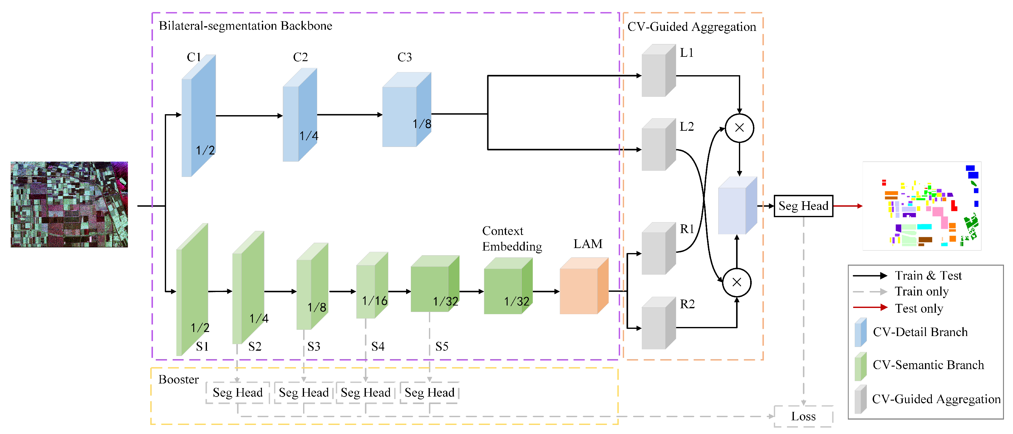
The architecture of LAM-CV-BiSeNetV2 is shown in Figure 1. The LAM-CV-BiSeNetV2 mainly contains three components: the bilateral-segmentation backbone in the purple dashed box, the aggregation layer in the orange dashed box, and the booster part in the yellow dashed box. The bilateral-segmentation backbone includes a CV-Detail Branch and a CV-Semantic Branch. At the end of the CV-Semantic Branch, the designed LAM is placed.

To further introduce the proposed structure of the network, CV-Detail Branch, CV-Semantic Branch, CV-Bilateral Guided Aggregation, CV-SegHead, LAM, computing method of complex network, and training strategy are presented in this section, respectively. In addition, the selection of the loss function is also introduced.

2.1. LAM-CV-BiSeNetV2 Structure

In the proposed method, we design the LAM-CV-BiSeNetV2 for PolSAR image segmentation. As shown in Figure 1, LAM-CV-BiSeNetV2 has a bilateral-segmentation structure consisting of CV-Detail Branch and CV-Semantic Branch, as well as a CV-Guided Aggregation Layer. The specific composition of these components is presented in Figure 2.

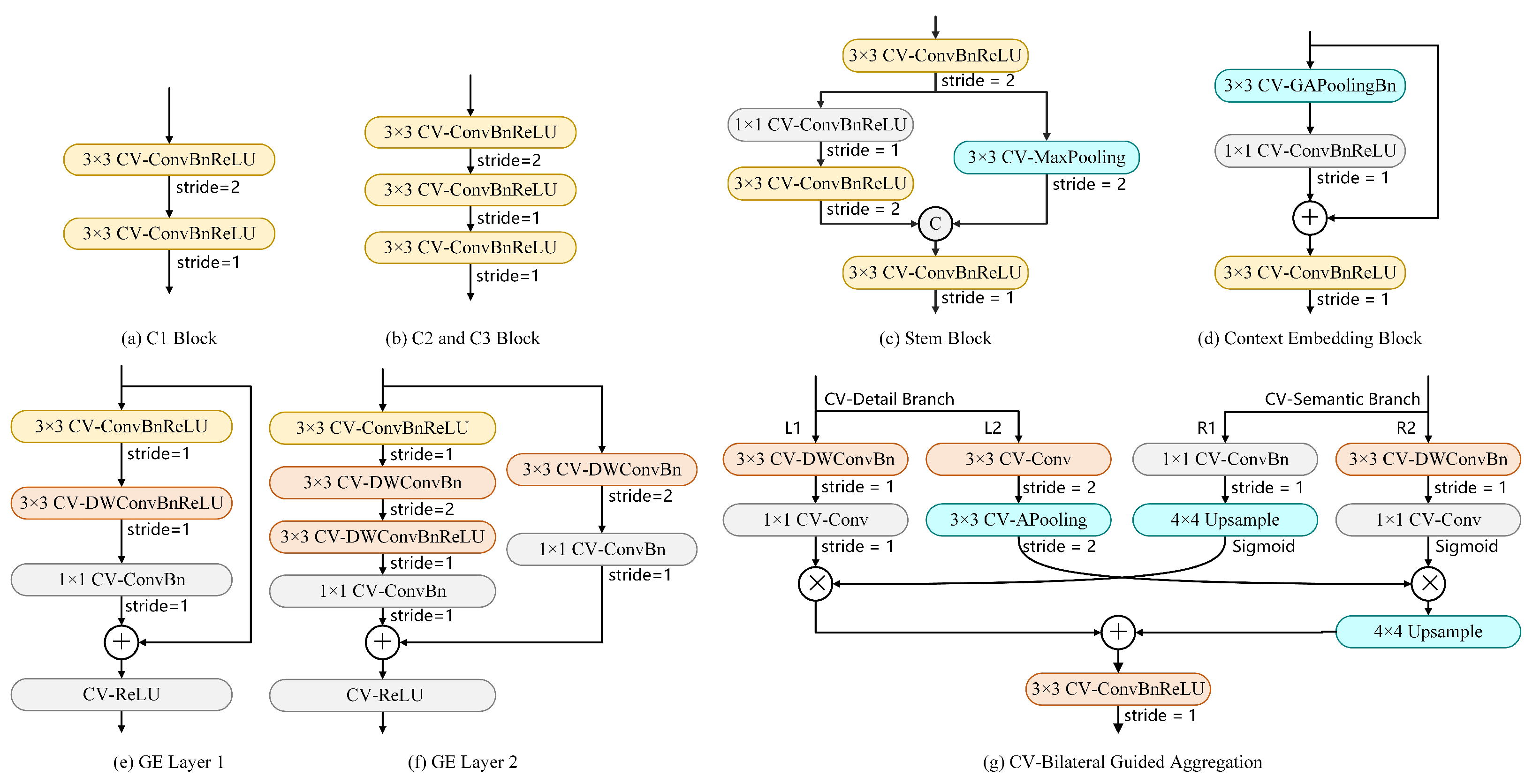
The CV-Detail Branch is designed to capture the spatial details with wide channels and shallow layers, which includes three stages: C1–C3. The composition of C1–C3 is shown in Figure 2a,b, which is composed of 3 × 3 CV-ConvBnReLU with a step size of 2 or 1 in series, and each CV-ConvBnReLU signifies a concatenation of CV-Conv, CV-Batch Normalization, and CV-ReLU.

The CV-Semantic Branch is used to extract the categorical semantics with narrow channels and deep layers, containing stages S1–S5 and the Context Embedding block. Among them, S1 and S2 form the Stem Block. S3 and S4 are both sequentially connected by GE Layer 2 and GE Layer 1. S5 is composed of one GE Layer 2 and three GE Layer 1 connected in series. The structures of Stem Block and Context Embedding are shown in Figure 2c,d. The utilization of the global average pooling layer enhances the perception of context. The structures of GE Layer 1 and GE Layer 2 are shown in Figure 2e,f. The use of 3 × 3 Conv effectively extracts high-dimensional features, 3 × 3 DWConv performs a separate convolution on each output channel, and 1 × 1 Conv performs low-capacity projection on the number of output channels.

The LAM is located at the output of the CV-Semantic Branch to further optimize semantic features. These two types of features are finally merged by the CV-Guided Aggregation Layer, which is explained in Figure 2g. In the CV-Guided Aggregation Layer, R1 and R2 align the semantic features with the detail features in space through CV-upsampling, and use 1x1 CV-Conv and CV-Sigmoid activation to allow the semantic features to focus on key areas at high resolution. L1 and L2 reduce the resolution through CV-APooling to match the scale of the semantic features. Feature fusion is performed using element-by-element multiplication, so that the semantic features can be adapted at the high-resolution. level. The booster part, composed of some auxiliary segmentation heads in the gray dashed boxes at the different stages of the CV-Semantic Branch, is used to improve the segmentation performance and design the training strategy. After information aggregation through the CV-Guided Aggregation Layer, it is processed by a SegHead block as the final output of the network.

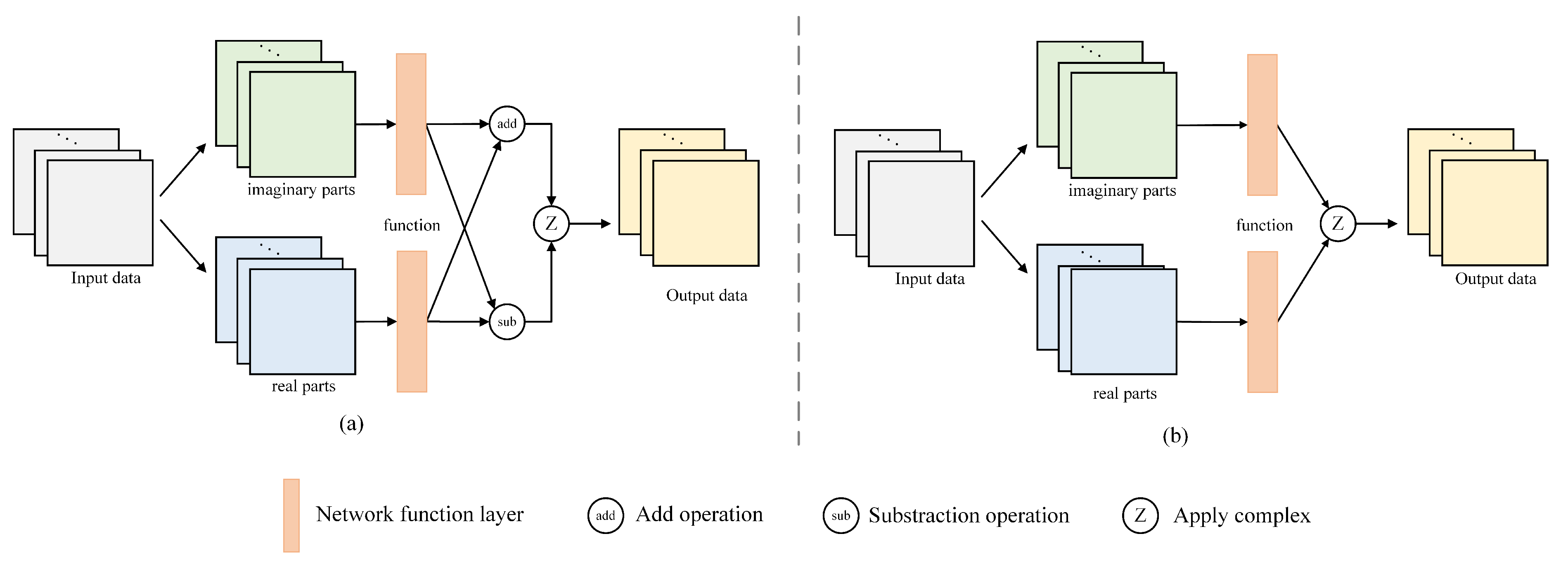
All operations in LAM-CV-BiSeNetV2, including convolution, batch normalization, pooling operations, and activation functions, are complex-valued, and the specific process of calculation is illustrated in Figure 3. Among them, CV-DWConv refers to complex-valued depthwise convolution, which has fewer parameters and less computation. In the CV-Semantic Branch, the combined use of CV-Conv and CV-DWConv improves the operating efficiency and flexibility of the model while ensuring model performance. The method of CV activation functions, CV-Batch Normalization, and CV-Conv are applied [50]. Specifically, the implementation follows a widely adopted approach in complex-valued neural networks, where real and imaginary components are processed separately but jointly maintain complex consistency. Although the operations are computed on real-valued tensors, the real and imaginary parts are updated in a coordinated manner to ensure that both amplitude and phase information are preserved. Furthermore, the mathematical formula of CV-DWConv, CV-Upsampling, and CV-Pooling operations are designed and explained below.

Firstly, some symbols in the formula are defined. The ith $\left(i=1,2,\dots ,I\right)$ complex input feature map is denoted as $F_i$, where I is the number of complex input feature channels. The jth $\left(j=1,2,\dots ,J\right)$ complex output feature map is marked as $O_j$ and J is the count of complex output feature channels. The position of pixels in the feature map is recorded as $\left(x,y\right)$ and the pixel coordinates in each convolution kernel are denoted as $\left(u,v\right)$. Then, the specific announcement and explanation are as follows.

(1)

CV-DWConv: In a depthwise convolution, each input channel is convolved with a separate filter. This means the number of input feature channels is the same as the total of filters and output feature channels. The equation of CV-DWConv is expressed as (1), where $W_i$ means the ith convolution kernel in size of $k_i\times k_i$ and $s\left(s\ge 1\right)$ represents the stride.

$$O_i\left(x,y\right)=\sum _{u=0}^{k_1-1}\sum _{v=0}^{k_2-1}{W}_i\left(u,v\right)F_i\left(x·s+u,y·s+v\right)$$

(1)

(2)

CV-Pooling: As shown in Figure 2c,d, CV max pooling is used in the Stem Block, and CV global average pooling is applied in the Context Embedding Block. In Figure 2g and Figure 4, a CV average pooling and a CV adaptive average pooling are adopted in CV-Bilateral Guided Aggregation and LAM, respectively. CV max pooling first calculates the amplitude of each complex number in the pooling window, finds the complex element $F_i^{\prime }$ with the largest amplitude first. Then, according to the phase relationship angle $\theta$ of $F_i$, the complex output is obtained. The phase angle ${\theta }_i$ of each complex feature $F_i=x_i+j{y}_i$ is computed as (3). The specific calculation steps are as shown in (2) and (4), where m denotes pooling size and s is the stride, $abs(·)$ means taking the absolute value. The other pooling operations are the same as the average pooling process [34].

$$F_i^{\prime }=\underset{u,v=0,\dots ,m-1}{max}\left|F_i\left(x·s+u,y·s+v\right)\right|$$

(2)

$${\theta }_i=arctan\left({\displaystyle \frac{y_i}{x_i}}\right)$$

(3)

$$O_i=cos\left({\theta }_i\right)·F_i^{\prime }+jsin\left({\theta }_i\right)·F_i^{\prime }$$

(4)

(3)

CV-Upsampling: The CV upsampling layer enlarges the spatial resolution of the complex feature maps. Specifically, the real and imaginary parts are independently interpolated using bilinear interpolation, and then recombined to reconstruct the complex-valued output. If each pixel in the feature map is expanded to a size of $k\times k$, the formula is expressed as (5), where $m,n\in \left[0,1,\dots ,k-1\right]$. As shown in Figure 2g, the CV upsampling operation is mainly used in CV-Bilateral Guided Aggregation and SegHead. Compared with the original structure, a CV relu operation is added to the final output to optimize the network results.

$$F^{\prime }(x·k+m,y·k+n)=\mathrm{Interp}\left(\Re \left(F\right(x,y\left)\right)\right)+j\mathrm{Interp}\left(\Im \left(F\right(x,y\left)\right)\right)$$

(5)

2.2. Structure of Lightweight Attention Module

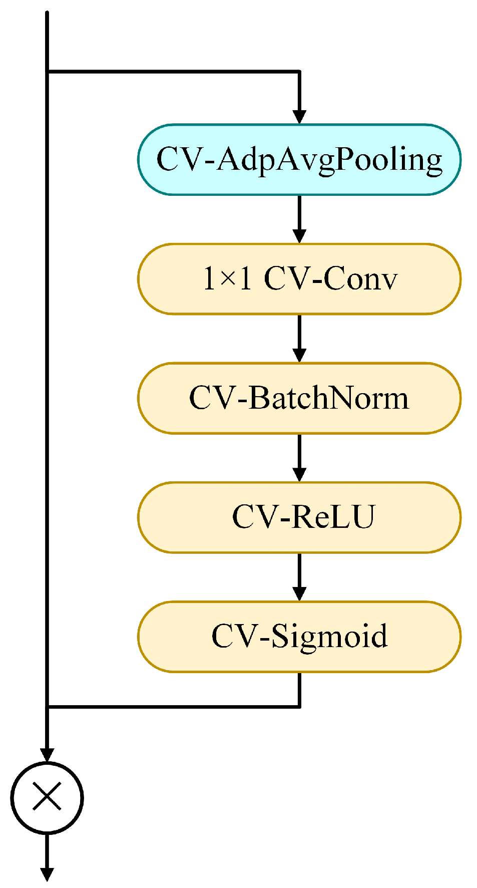
At the end of CV-Semantic Branch, a lightweight attention module (LAM) is designed to refine the semantic features in the complex domain. It performs channel-wise attention weighting based on the global response statistics of each polarization channel, thereby balancing their contributions to the overall semantic representation. As presented in Figure 4, adaptive average pooling is employed to capture global information and improve the robustness of the model to changes in input size. Then, a concatenation of CV-Conv, CV-Batch Normalization, and CV-ReLU is designed to extract more spatial features, which are combined with features from CV-Semantic Branch later. This process acts as an optimization of the output features of the CV-Semantic Branch. This structure is similar to SENet [51], but LAM uses convolutional layers for feature transformation, which can retain more spatial information. Because of the lightweight structure, LAM can improve model performance while demanding negligible computation cost.

2.3. Training Strategy

In order to optimize the training effect, a booster training strategy is utilized in this experiment, which uses different methods to calculate the loss function during training and validation. SegHead exists in different stages of the CV-Semantic Branch and the final output of BiSeNetV2. This is an auxiliary segmentation module that contains a 3 × 3 CV-ConvBnReLU with 0.1 dropout and a 1 × 1 CV-Conv with CV-Upsampling. During the training stage, in addition to the final output of the network, the S2–S5 stages of the CV-Semantic Branch are also processed by SegHead and calculated into the loss function. The outputs of all SegHeads are computed by the loss function so that the features of different stages can be utilized reasonably for training. During validation, only the final network output contributes to the loss function. This flexible training strategy allows for capturing more adequate information to participate in the loss computation during training, while reducing the amount of computation in the validation phase.

In detail, the AdamW algorithm with a 0.0001 learning rate and a 0.1 weight decay [52] is used to train the model for 200 epochs. In addition, an early stopping strategy is chosen for the training process, and the batch size is 8. When the performance on the validation stage does not improve for 30 consecutive epochs, the training is terminated early to avoid overfitting of the model on the training set, and the model parameters are saved only when the loss on the validation stage reaches the current minimum value. These hyperparameters are chosen based on prior studies and preliminary experiments, which showed that this configuration achieves a stable convergence and good generalization performance.

2.4. Loss Function

The cross-entropy [53] is selected as the loss function of LAM-CV-BiSeNetV2, which is an ideal selection for multi-category classification tasks. The loss in the training stage contains the outputs of all segheads, while the loss in the validation stage only uses the final output of the network. The overall loss function formula is showed in (6), where $q_n\left(x,y\right)$ means the ground-truth label at $\left(x,y\right)$, $p_n\left(x,y\right)$ represents the predicted label of $\left(x,y\right)$, $\mathit{h}$ denotes the output of seghead of different paths $h\in \left(1,2,\dots ,H\right)$, $H=5$, and the Hth path is the final output of the network.

$$Loss=\left\{\begin{array}{c}-\sum _{h=1}^H\sum _{\left(x,y\right)}\sum _{n=1}^N{q}_n\left(x,y\right)ln{p}_n\left(x,y\right)train\hfill \\ -\sum _{x,y}\sum _{n=1}^N{q}_{n}ln{p}_n\left(x,y\right){|}_{h=H}validation\hfill \end{array}\right.$$

(6)

3. Datasets and Evaluation Metrics

In this section, three sets of fully PolSAR datasets are introduced to demonstrate the effectiveness of LAM-CV-BiSeNetV2, including two Flevoland datasets and one San Francisco dataset. Then, the process of data preprocessing and the evaluation measures of semantic segmentation are presented.

3.1. Datasets

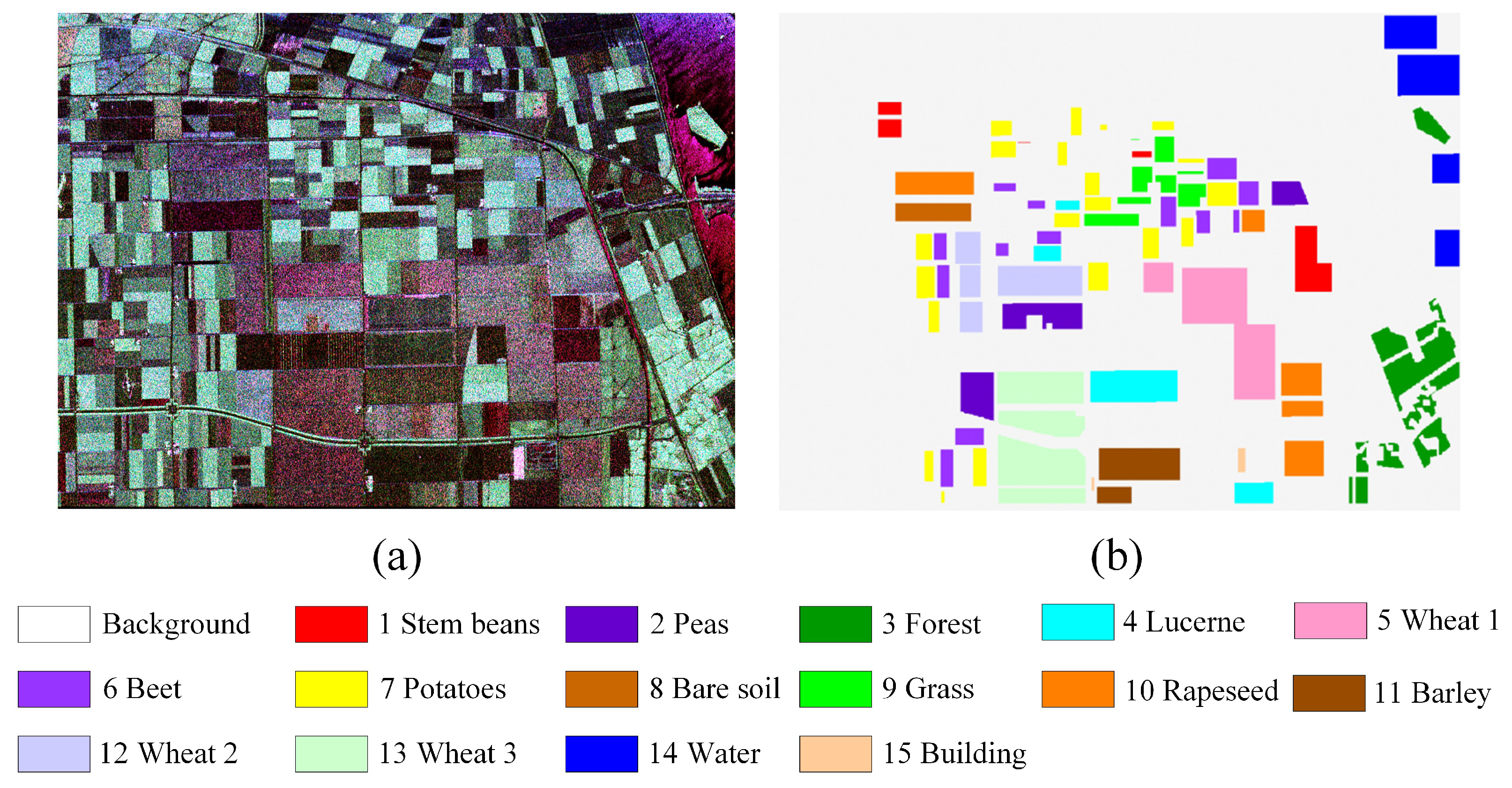
The first L-band full polarimetric Flevoland dataset was acquired by the AIRSAR airborne platform in August 1989. There are a total of 15 types of land covers, namely stem beans, peas, forest, lucerne, three kinds of wheat, beet, potatoes, bare soil, grass, rapeseed, barley, water, and some buildings. Its pseudo color image obtained by Pauli decomposition in size of 1024 × 750 is shown in Figure 5a. The ground truth is presented in Figure 5b, where the white areas are considered as the background.

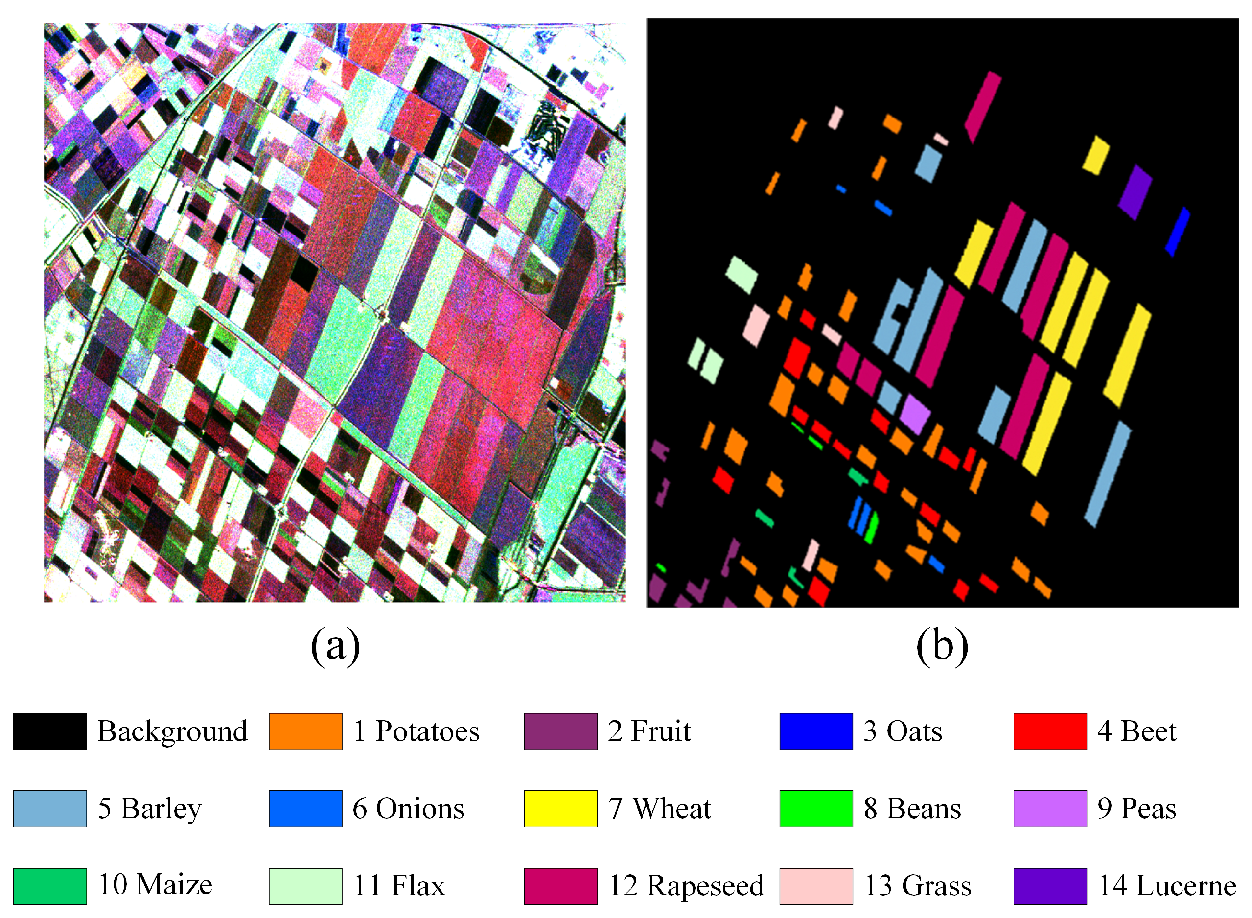
The second L-band full polarimetric Flevoland dataset was acquired by the AIRSAR airborne platform in 1991. There are 14 types of land covers in total, namely potatoes, fruit, oats, beet, barley, onions, wheat, beans, peas, maize, flax, rapeseed, grass, and lucerne. The pseudo color image obtained by Pauli decomposition in size of 1024 × 900 is shown in Figure 6a. The ground truth is presented in Figure 6b, where the black regions are regarded as the background.

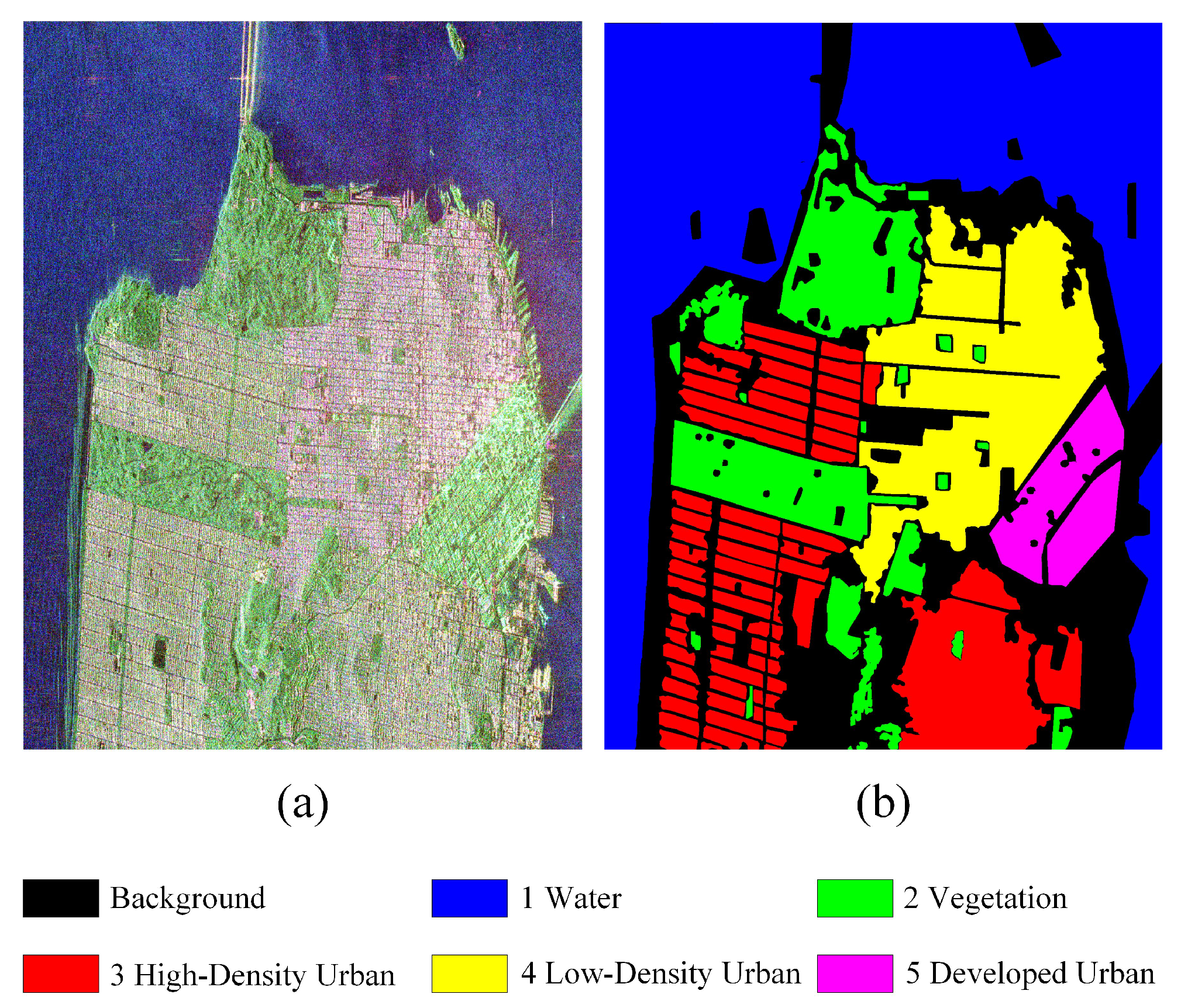
The third L-band full polarimetric San Francisco dataset was acquired by the AIRSAR airborne platform in 2008. There are five categories of objectives, namely water, vegetation, high-density urban, low-density urban, and developed urban. The pseudo color image formed by Pauli decomposition in size of 1800 × 1380 is shown in Figure 7a. The ground truth is shown in Figure 7b, where the black areas are regarded as the background.

3.2. Data Preprocessing

For PolSAR data, H and V stand for horizontal and vertical polarization, respectively. The information of polarimetric SAR is mainly represented by the coherence matrix $\mathit{T}$ and the covariance matrix $\mathit{C}$, both of which are hermitian symmetric matrices. In the single-station backscattering system, $S_{HV}$ is equal to $S_{VH}$ according to the reciprocity theory. Therefore, the polarimetric coherence matrix can be simplified and presented by (7)

$$T=\left[\begin{array}{ccc}{T}_{11}& T_{12}& T_{13}\\ T_{21}& T_{22}& T_{23}\\ T_{31}& T_{32}& T_{33}\end{array}\right]$$

(7)

where $T_{11}$, $T_{22}$, $T_{33}$ are real-valued and $T_{12}$, $T_{13}$, $T_{23}$ are complex-valued.

For LAM-CV-BiSeNetV2, the upper triangular matrix $\left\{T_{11},T_{22},T_{33},T_{12},T_{13},T_{23}\right\}$ of the $\mathit{T}$ matrix is taken as the 6-channel input. For the real-valued networks in Section 4, the $\mathit{T}$ matrix is processed into a real vector, and the 6-channel input data [34] is expressed by (8) sequentially.

$$\left\{\begin{array}{c}A=10{log}_{10}\left(SPAN\right)\hfill \\ B=T_{22}/SPAN\hfill \\ C=T_{33}/SPAN\hfill \\ D=|T_{12}|/\sqrt{T_{11}·T_{22}}\hfill \\ E=|T_{13}|/\sqrt{T_{11}·T_{33}}\hfill \\ F=|T_{23}|/\sqrt{T_{22}·T_{33}}\hfill \\ SPAN=T_{11}+T_{22}+T_{33}\hfill \end{array}\right.$$

(8)

In order to obtain sufficient datasets for experiments, the following augmentation operations are performed on the inputs of RV and CV. The original image is rotated $\left\{90,180,270\right\}$ degrees as well as horizontally and vertically separately, then these five images are cropped with a 64 × 64 size sliding window in steps of 64, respectively. After dividing the training set and validation set into a ratio of 6:4, the numbers of training and validation samples of the three datasets are presented in

Table 1. Training and validation sets.

Dataset	Train	Validation
Flevoland dataset 1	351	234
Flevoland dataset 2	507	338
San Francisco dataset	1482	988

.

3.3. Evaluation Metrics

In Section 4, mean intersection over union (MIoU), frequency weighted intersection over union (FWIoU), overall accuracy (OA), and mean pixel accuracy (MPA) are utilized to estimate the performance of different methods. MIoU calculates the intersection over union (IoU) of each category and takes the average, which effectively measures the overall performance of the segmentation results by focusing on the intersection of each category’s prediction and the true segmentation. MPA calculates the average pixel accuracy (PA) of all categories based on pixel-level accuracy. FWIoU takes into account the frequency of each class in the dataset and uses these frequencies to take a weighted average of the IoU for each class. OA measures the proportion of samples correctly classified by the model in the total samples. The Kappa coefficient is used to measure the consistency between the classification results and the true label, taking into account the “accidental consistency” situation. The formulas for these five evaluation metrics are as follows

$$MIoU={\displaystyle \frac{1}{N+1}}\sum _{i=0}^N{\displaystyle \frac{p_{ii}}{p_{ij}+{\sum }_{j=0}^N{p}_{ji}-p_{ii}}}$$

(9)

$$MPA={\displaystyle \frac{1}{N+1}}\sum _{i=0}^N{\displaystyle \frac{p_{ii}}{{\sum }_{j=0}^N{p}_{ij}}}$$

(10)

$$FWIoU={\displaystyle \frac{1}{N+1}}\sum _{i=0}^N{\displaystyle \frac{\left({\sum }_{j=0}^N{p}_{ij}\right)p_{ii}}{{\sum }_{j=0}^N{p}_{ij}+{\sum }_{j=0}^N{p}_{ji}-p_{ii}}}$$

(11)

$$OA={\displaystyle \frac{{\sum }_{i=0}^N{p}_{ii}}{{\sum }_{i=0}^N{\sum }_{j=0}^N{p}_{ij}}}$$

(12)

$$Kappa={\displaystyle \frac{OA-p_e}{1-p_e}},p_e={\displaystyle \frac{{\sum }_{i=0}^N\left({\sum }_{j=0}^N{p}_{ij}\right)\left({\sum }_{j=0}^N{p}_{ji}\right)}{{\left({\sum }_{i=0}^N{\sum }_{j=0}^N{p}_{ij}\right)}^2}}$$

(13)

where $\mathit{N}$ denotes the total number of categories and $p_{ij}$ represents the element at position $\left(i,j\right)$ in the confusion matrix. $\left({\sum }_{j=0}^N{p}_{ij}\right)$ and $\left({\sum }_{j=0}^N{p}_{ji}\right)$ means the sum of the row $\mathit{i}$ and column $\mathit{j}$ in the confusion matrix, respectively.

4. Experiments

In this section, we study the performance improvement of complex operations and evaluate LAM for optimizing segmentation results by comparing it with other attention mechanisms at first. Then, semantic segmentation experiments are conducted on three PolSAR datasets, and the performance of LAM-CV-BiSeNetV2 is compared with that of five other RV networks, namely FCN [54], U-Net [55], DeepLabV3+ [56], and ICNet [49] to verify the advantages of LAM-CV-BiSeNetV2. Among them, the FCN, UNet, and DeepLabV3+ follow an encoder–decoder structure. A kind of multi-scale cascade structure is used by ICNet.

4.1. Evaluation of LAM

In our method, a lightweight attention module (LAM) is designed to optimize the extraction of semantic details and features, which is placed at the end of the CV-Semantic Branch. In order to verify the improvement of LAM on segmentation performance, comparative experiments are carried out on three PolSAR datasets for BiSeNetV2, CV-BiSeNetV2, and LAM-CV-BiSeNetV2. Furthermore, in order to demonstrate the effectiveness of LAM compared to other attention modules, CBAM [43], SEAM [57], and Self-Attention [58] are placed at the same position in the network, and the same experiments are conducted.

CBAM is a classic attention module that combines channel attention and spatial attention and is often used to optimize semantic segmentation. SEAM uses equivariance and attention mechanisms to improve the performance of semantic segmentation models, and is applicable to both supervised and weakly supervised conditions. The self-attention mechanism enables the model to pay more attention to global information rather than just local neighborhoods during feature extraction. Compared with these classic attention mechanisms, LAM can capture global information, refine features further, and integrate them with the features of the previous stage to achieve better segmentation results.

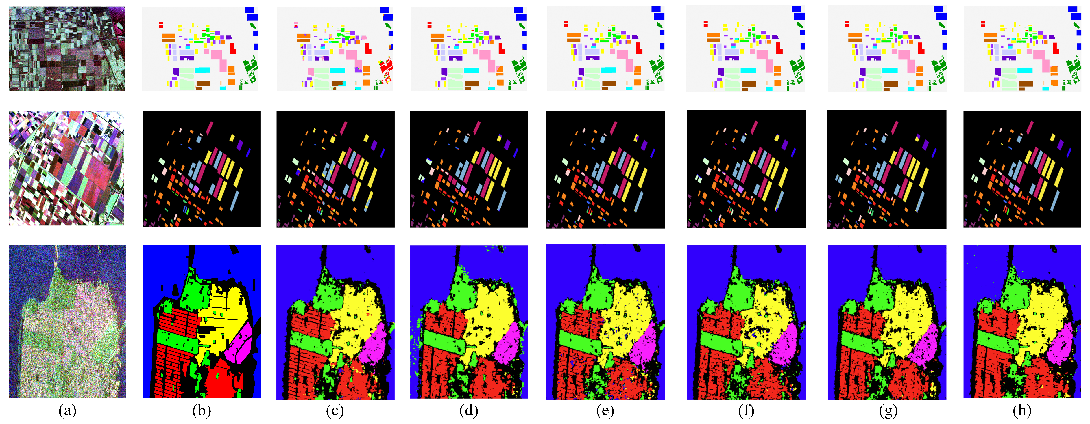
The MPA, MIoU, FWIoU, and OA obtained by BiSeNetV2, CV-BiSeNetV2, CBAM-CV-BiSeNetV2, SEAM-CV-BiSeNetV2, Self Attention-CV-BiSeNetV2, and LAM-CV-BiSeNetV2 on three datasets are shown in

Table 2. Evaluation of LAM.

Method	Flevoland Dataset 1				Flevoland Dataset 2				San Francisco Dataset
	MPA	MIoU	FWIoU	OA	MPA	MIoU	FWIoU	OA	MPA	MIoU	FWIoU	OA
BiSeNetV2	80.34	69.46	69.80	80.58	77.28	68.27	79.33	87.92	79.47	65.91	68.02	79.82
CV-BiSeNetV2	98.68	96.40	97.18	98.54	82.51	74.47	91.91	95.14	82.34	67.71	68.53	80.48
CBAM-CV-BiSeNetV2	99.42	98.86	99.02	99.50	82.29	77.72	93.62	96.18	81.22	66.89	68.02	80.22
SEAM-CV-BiSeNetV2	99.26	99.28	99.39	99.48	79.05	70.80	90.58	94.38	81.01	67.38	68.07	80.16
Self Attention-CV-BiSeNetV2	98.91	97.51	97.91	98.93	79.46	71.97	89.97	93.98	81.51	68.43	70.28	81.61
LAM-CV-BiSeNetV2	99.71	99.31	99.51	99.76	85.04	81.83	95.11	97.13	83.56	70.08	70.98	82.24

. CV-BiSeNetV2 represents the complex-valued BiSeNetV2 network without any attention mechanism. The frames per second (FPS) of CV-BiSeNetV2 with different attention mechanisms are shown in

Table 3. Frames per second of model with different attention.

Method	Flevoland Dataset 1	Flevoland Dataset 2	San Francisco Dataset
CBAM-CV-BiSeNetV2	2.19	2.07	1.74
SEAM-CV-BiSeNetV2	1.84	1.99	1.81
Self Attention-CV-BiSeNetV2	1.59	1.99	1.90
LAM-CV-BiSeNetV2	2.31	2.20	1.85

. The segmentation results of all experiments are shown in Figure 8a–h. Based on the above experiments, complex-valued calculation makes it utilize the phase information in polarimetric SAR data fully and extract more polarization features, thereby achieving better classification results.

It can be observed from Table 2 that the performance of BiSeNetV2, CV-BiSeNetV2, and LAM-CV-BiSeNetV2 is improved successively. Compared to BiSeNetV2, CV-BiSeNetV2 shows an 18.34% improvement in MPA, 26.94% improvement in MIoU, 27.38% improvement in FWIoU, and 17.96% improvement in OA on the Flevoland Dataset 1 dataset. On the Flevoland Dataset 2 dataset, CV-BiSeNetV2 shows an increase of 5.23% in MPA, 6.2% in MIoU, 12.58% in FWIoU, and 7.22% in OA. On the San Francisco Dataset, it shows a 2.87% increase in MPA, a 1.8% increase in MIoU, a 0.51% increase in FWIoU, and a 0.66% increase in OA. Overall, CV operation has significantly improved network performance.

In the experiment comparing the attention mechanism to CV-BiSeNetV2, LAM has the best effect on improving the network. On Flevoland Dataset 1, LAM improves the MPA of CV BiSeNetV2 by 1.03%, MIoU by 2.91%, FWIoU by 2.33%, and OA by 1.22%; On Flevoland Dataset 2, LAM results in a 2.53% increase in MPA, a 7.36% increase in MIoU, a 3.2% increase in FWIoU, and a 1.99% increase in OA. On the San Francisco Dataset, with the addition of LAM, MPA increased by 1.22%, MIoU by 2.37%, FWIoU by 2.45%, and OA by 1.76%. In addition, on Flevoland dataset 1, CBAM, SEAM, and Self Attention all have a positive effect on the performance improvement of CV-BiSeNetV2, while on Flevoland dataset 2, SEAM and Self Attention have a negative effect, and on the San Francisco Dataset, SEAM has a negative effect, indicating that the attention module has an unstable effect on network performance. However, in all experiments, LAM shows a positive effect, which to some extent proves the adaptability and stability of LAM relative to the network.

FPS is the inverse of the time required for model inference, and a higher FPS indicates a faster inference of the network. In the experiment, the FPS was calculated by inferring and predicting each complete PolSAR image 100 times. Table 3 shows that LAM-CV-BiSeNetV2 has the highest FPS on Flevoland dataset1 and Flevoland dataset2, and is close to Self Attention-CV-BiSeNetV2, which has the highest FPS, in the San Francisco Dataset. In general, LAM is more lightweight compared to other attention mechanisms.

Overall, the CV operation significantly improves the classification accuracy, LAM further improves the performance of the model in a relatively lightweight manner, and LAM-CV-BiSeNetV2 has the best classification performance.

4.2. Experiment on Flevoland Dataset 1

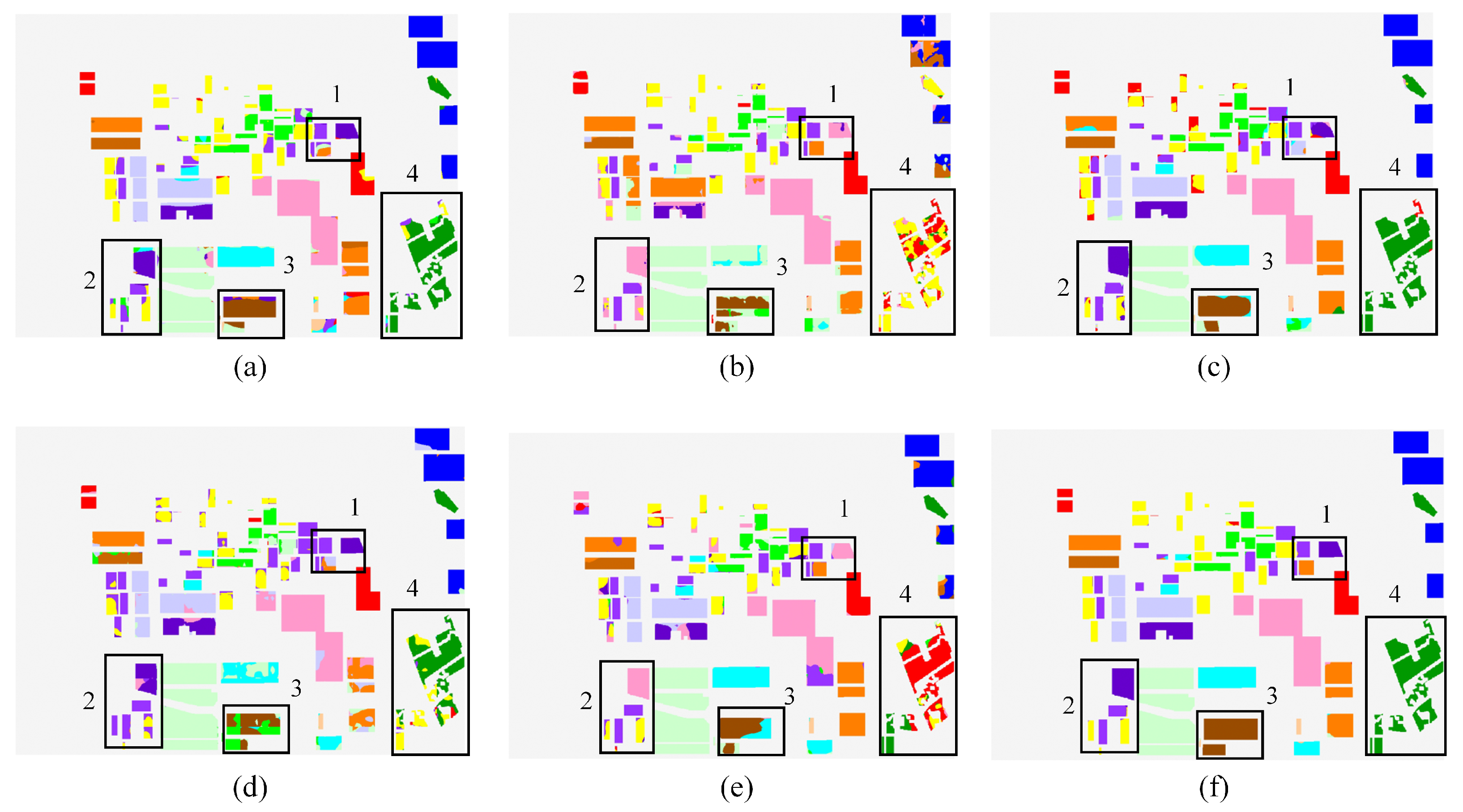
For Flevoland dataset 1, the semantic segmentation results of LAM-CV-BiSeNetV2 and other RV networks are presented in Figure 9a–f, respectively. In each figure of different networks, there are four parts marked by black boxes.

The region framed by black box 1 includes peas, beets, and rapeseed, and these three categories are relatively balanced in the sample. Some rapeseed is misclassified into beet by FCN; peas are covered as wheat 1 by U-Net and BiSeNetV2; rapeseed is mixed with wheat 2 by DeepLabV3+ and ICNet. These errors arise mainly from similar polarimetric backscattering characteristics among these crops. The region framed by black box 2 includes peas, beets, and potatoes, and these three categories are also relatively balanced in the sample. Some parts of peas and beets are mixed with other categories by FCN; peas and potatoes are misclassified as wheat 1 by U-Net; peas are mixed with wheat 1, and potatoes are mixed with beets by DeepLabV3+ and ICNet; peas are misclassified as wheat 1 by BiSeNetV2. Such misclassifications often occur in areas with blurred field boundaries. In the region of barley framed by black box 3 barley, which is partially mixed with wheat 3 by FCN; partially misclassified as grass and wheat 3 by U-Net; partially misclassified as grass by ICNet, and partially mixed with wheat 3 and lucerne by DeepLabV3+ and BiSeNetV2. This confusion stems from similar scattering intensities. In the region of forest framed by black box 4, a small part is mixed with other categories by FCN and DeepLabV3+; a considerable part is misclassified as stem beans and potatoes by U-Net, ICNet, and BiSeNetV2. This is mainly due to similar surface roughness and volume scattering patterns. Since barley and forest are less represented and more spatially clustered in the dataset, they pose a greater challenge for the model to generalize effectively.

In contrast, for these marked regions, our LAM-CV-BiSeNetV2 captures the phase coupling between real and imaginary components while the attention mechanism highlights crop boundaries, effectively separating visually and physically similar classes. The performance of LAM-CV-BiSeNetV2 is much better than other networks.

In addition, the segmentation performances of different methods are presented in

Table 4. Comparison of classification accuracy in Flevoland Dataset 1.

Class	FCN	U-Net	DeepLabV3+	ICNet	BiSeNetV2	LAM-CV-BiSeNetV2
Stem beans	88.43	97.44	99.99	97.51	73.54	99.90
Peas	84.43	30.21	92.73	88.15	31.88	99.99
Forest	90.64	4.2	96.27	72.91	25.49	99.99
Lucerne	78.28	16.78	77.68	74.73	97.44	98.15
Wheat 1	97.11	97.72	99.68	94.80	86.34	99.99
Beet	77.47	96.91	95.44	97.65	99.99	99.08
Potatoes	95.09	81.78	76.73	61.56	77.73	99.78
Bare soil	99.99	91.39	99.80	80.70	91.88	99.99
Grass	97.05	70.97	97.27	65.42	87.33	99.79
Rapeseed	81.09	91.14	85.64	71.25	96.09	99.19
Barley	75.32	61.65	86.74	55.11	67.50	99.99
Wheat 2	96.80	1.46	96.69	95.44	99.16	99.99
Wheat 3	96.02	99.94	99.68	99.89	99.97	99.98
Water	98.96	62.67	99.97	94.95	88.57	99.99
Building	65.76	80.04	92.44	80.67	82.14	94.80

and

Table 5. Performance of different methods in Flevoland Dataset 1.

Method	MPA	MIoU	FWIoU	OA	Kappa
FCN	88.16	77.42	83.29	90.51	89.64
U-Net	65.62	48.70	46.79	65.84	62.41
DeepLabV3+	93.16	87.04	88.00	93.20	92.58
ICNet	82.05	93.00	73.21	83.73	82.20
BiSeNetV2	80.34	69.46	69.80	80.58	78.83
LAM-CV-BiSeNetV2	99.44	98.27	99.46	99.68	99.42

. The classification accuracy obtained by FCN, U-Net, DeepLabV3+, ICNet, BiSeNetV2, and LAM-CV-BiSeNetV2 in different categories of Flevoland Dataset 1 is shown in Table 4. Apart from stem beans, our method achieves the highest classification accuracy. The MPA, MIoU, FWIoU, OA, and Kappa obtained by these semantic segmentation networks on Flevoland Dataset 1 are presented in Table 5. It can be observed that our method achieves the highest MPA, MIoU, FWIoU OA, and Kappa. In addition, LAM optimization and complex-valued calculation make the performance of LAM-CV-BiSeNetV2 surpass that of FCN and ICNet, which are better than the original BiSeNetV2.

According to the segmentation results in Figure 9, Table 4 and Table 5, it can be analyzed that LAM-CV-BiSeNetV2 has the best classification performance in this semantic segmentation experiment.

4.3. Experiment on Flevoland Dataset 2

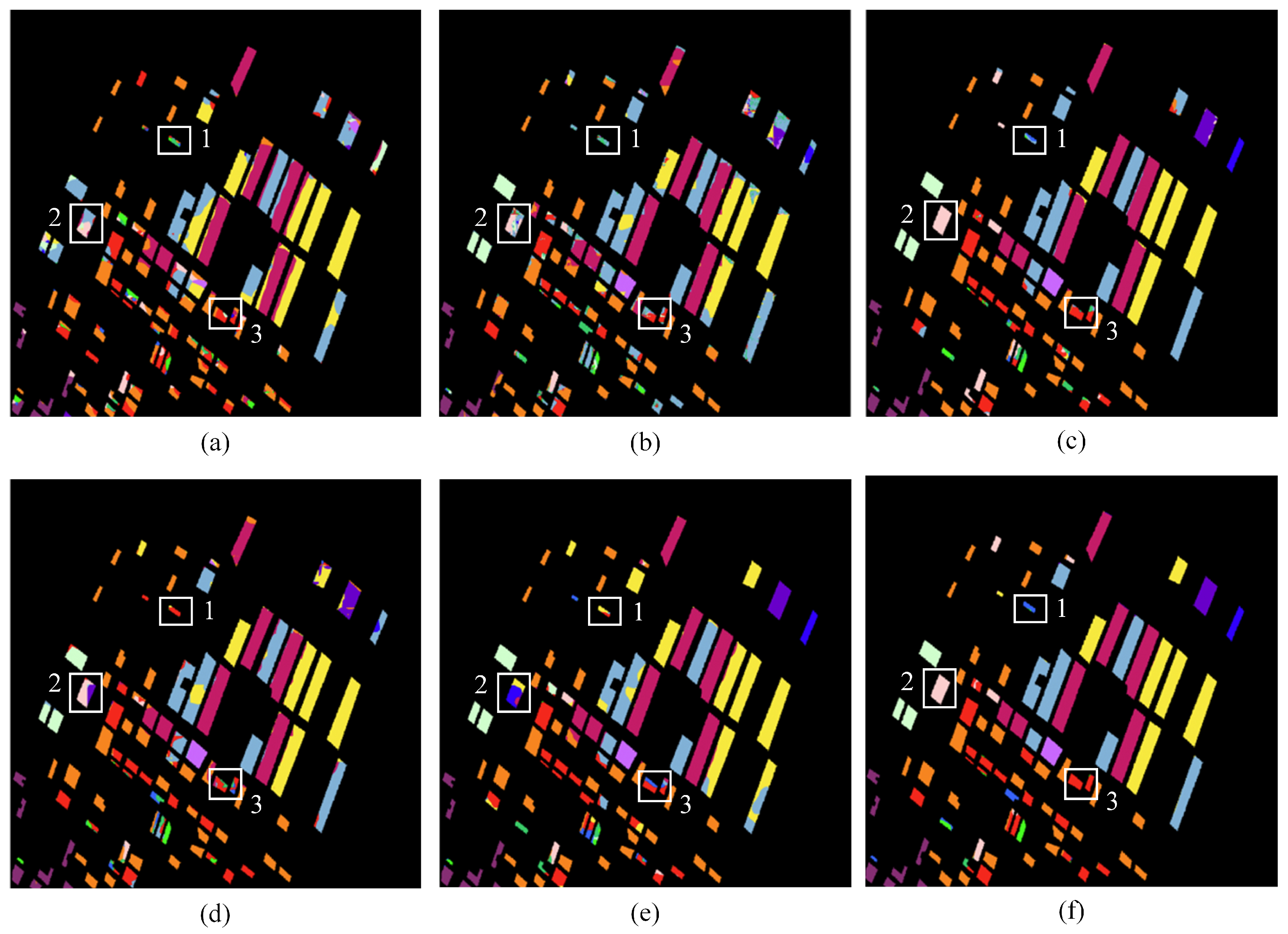
For Flevoland dataset 2, the semantic segmentation results of LAM-CV-BiSeNetV2 and other RV networks are presented in Figure 10a–f, respectively. In each figure of different networks, there are three parts marked by white boxes.

In the region framed by white box 1, onions are mixed with other types of crops by FCN, U-Net, and DeepLabV3+; misclassified as beet and wheat by ICNet and BiSeNetV2. mainly due to the high similarity in backscattering responses between these classes and the limited discriminative power of their real-valued features. In the region framed by white box 2, grass is partially covered by other categories by FCN and U-Net; partially misclassified as lucerne by ICNet; completely misclassified as wheat, oats, and beets by BiSeNetV2; classified correctly by DeepLabV3+ and LAM-CV-BiSeNetV2, suggesting that these models struggle with weak backscattering and irregular spatial boundaries. Furthermore, onions and grass account for a relatively small proportion of the samples in the dataset, which makes them more difficult to classify accurately. In the region framed by white box 3, all five real-valued networks partially misclassify beet, which can be attributed to the similar polarimetric signatures between beet and neighboring crops.

LAM-CV-BiSeNetV2 achieves accurate classification because the combination of complex-valued feature encoding and lightweight attention allows better separation of crops with similar scattering characteristics.

The classification accuracy of FCN, U-Net, DeepLabV3+, ICNet, BiSeNetV2, and LAM-CV-BiSeNetV2 in 14 categories of Flevoland Dataset 2 is shown in

Table 6. Comparison of classification accuracy in Flevoland Dataset 2.

Class	FCN	U-Net	DeepLabV3+	ICNet	BiSeNetV2	LAM-CV-BiSeNetV2
Potatoes	68.68	88.28	99.31	97.05	97.61	99.99
Fruit	76.11	83.96	99.52	99.70	99.79	99.99
Oats	0.00	44.05	99.98	19.08	99.99	99.99
Beet	35.60	64.86	81.62	87.10	74.42	97.66
Barley	47.78	91.09	99.27	88.69	75.62	99.43
Onions	5.59	2.91	14.27	8.87	29.20	17.84
Wheat	60.05	80.94	93.17	96.64	95.79	99.77
Beans	10.89	40.02	51.76	68.58	26.16	62.85
Peas	17.06	91.34	99.07	97.31	99.95	99.99
Maize	5.82	67.75	21.94	24.81	54.81	16.28
Flax	12.41	98.81	99.93	93.93	99.99	99.99
Rapeseed	75.30	93.08	97.84	96.72	99.68	99.72
Grass	23.82	44.98	90.46	48.33	28.88	97.07
Lucerne	4.27	32.49	94.92	86.21	99.89	99.99

. Among the 14 categories, our method achieves the best classification results in 11 categories. For the other 3 categories, BiSeNetV2, ICNet, and U-Net achieved the highest accuracy of 29.2%, 68.58%, and 67.75% in the onions, beans, and maize, respectively. For the onions and maize categories, the number of samples is much less than that of other categories, and it is more difficult to obtain ideal classification results through training.

Furthermore, the evaluation metrics of different methods are shown in

Table 7. Performance of different methods in Flevoland Dataset 2.

Method	MPA	MIoU	FWIoU	OA	Kappa
FCN	41.17	31.67	54.02	68.97	63.03
U-Net	66.04	54.31	70.63	81.80	78.43
DeepLabV3+	81.64	76.56	89.07	93.59	86.34
ICNet	72.36	65.22	82.06	89.73	87.84
BiSeNetV2	77.28	68.27	79.33	87.92	85.70
LAM-CV-BiSeNetV2	85.04	81.83	95.11	97.13	96.61

. Our method achieves the highest MPA of 85.04%, MIoU of 81.83%, FWIoU of 95.11%, OA of 97.13%, and the Kappa of 96.61, all of which are better than the performance of FCN, U-Net, DeepLabV3+, ICNet, and BiSeNetV2.

Based on the above performance, LAM-CV-BiSeNetV2 has the best classification performance compared with the other five network models in this experiment.

4.4. Experiment on San Francisco Dataset

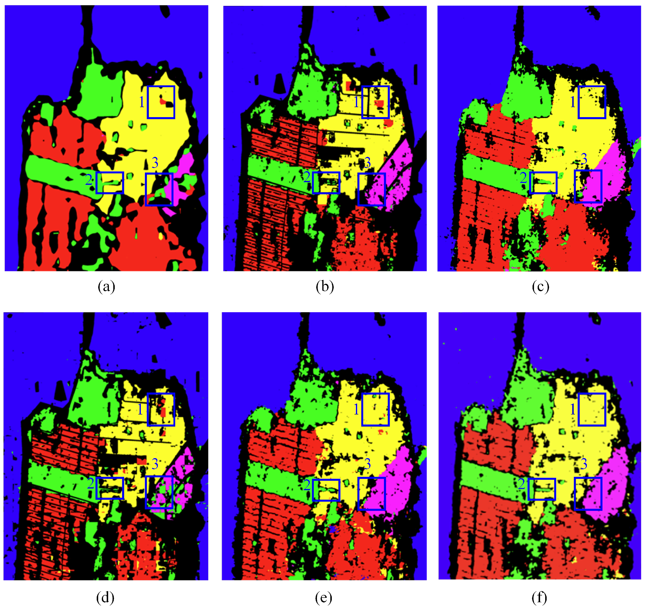
For the San Francisco dataset, the semantic segmentation results of LAM-CV-BiSeNetV2 and other RV networks are presented in Figure 11a–f, respectively. This dataset has a relatively balanced category distribution, which allows for a more direct and fair evaluation of the model’s classification capability. In each figure of different networks, there are three parts marked by blue boxes.

In the region framed by blue box 1, low-density urban is misclassified as high-density urban by FCN, U-Net, and ICNet partially; misclassified as high-density urban and vegetation by BiSeNetV2 partially; misclassified as background by DeepLabV3+ partially. Compared with the conditions of these networks, LAM-CV-BiSeNetV2 obviously achieves better classification results. These misclassifications mainly arise from the similar polarimetric responses between urban materials of different densities and the limited ability of real-valued networks to capture subtle scattering variations within heterogeneous urban structures. In the region framed by blue box 2, vegetation is not well classified by FCN, U-Net, DeepLabV3+, ICNet, and BiSeNetV2 partially. In the area of blue box 3 representing developed urban, other networks misclassified some developed urban areas as Vegetation, while U-Net and LAM-CV-BiSeNetV2 performed better. The problems are mainly due to the weak and spatially discontinuous scattering signals of vegetation in polarimetric SAR imagery.

In comparison, LAM-CV-BiSeNetV2 accurately distinguishes low-density from high-density urban regions and identifies the vegetation and developed urban areas.

The classification accuracy of FCN, U-Net, DeepLabV3+, ICNet, BiSeNetV2, and LAM-CV-BiSeNetV2 in different categories of the San Francisco dataset is shown in

Table 8. Comparison of classification accuracy in the San Francisco Dataset.

Class	FCN	U-Net	DeepLabV3+	ICNet	BiSeNetV2	LAM-CV-BiSeNetV2
Background	57.62	57.38	51.74	53.69	60.37	57.06
Water	95.09	98.55	98.20	96.46	97.06	98.35
Vegetation	69.03	80.59	80.68	88.46	77.54	79.15
High-Density Urban	83.71	73.39	89.27	64.05	72.20	79.09
Low-Density Urban	92.06	85.25	89.66	79.79	84.53	96.11
Developed Urban	31.79	84.14	80.92	51.64	85.11	85.33

. Different from Flevoland dataset 1 and Flevoland dataset 2, in the San Francisco dataset, since the area of background is similar to other categories, background is also shown as a category. Among these 6 categories, LAM-CV-BiSeNetV2 has the highest classification accuracy in categories of water, low-density urban, and developed urban. For the other 3 categories, BiSeNetV2, ICNet, and DeepLabV3+ have the best results for background, vegetation, and high-density urban classification, respectively.

The evaluation metrics of different methods are shown in

Table 9. Performance of different methods in San Francisco Dataset.

Method	MPA	MIoU	FWIoU	OA	Kappa
FCN	71.55	58.28	66.29	78.34	71.81
U-Net	79.88	66.39	68.27	80.03	73.95
DeepLabV3+	81.74	67.40	68.98	81.08	75.47
ICNet	72.35	58.48	63.74	76.05	68.82
BiSeNetV2	79.47	65.91	68.02	79.82	73.64
LAM-CV-BiSeNetV2	83.56	70.08	70.98	82.24	76.39

. It can be seen that LAM-CV-BiSeNetV2 has the highest MPA, MIoU, FWIoU, OA, and Kappa, which reach 83.56%, 70.08%, 70.98%, 82.24% and 76.39%, respectively, proving that our method has the best segmentation performance.

4.5. Experimental Summary

In the above four experiments, complex-valued operations and LAM are first evaluated to demonstrate their effects on improving network performance and show that LAM has a stable positive impact with a lightweight computational burden on network performance compared to the other three attention modules. Then, the comparative experiments with five real-valued networks on three data sets are conducted to verify the performance of our method compared with other networks. It can be concluded that LAM-CV-BiSeNetV2 can achieve the best classification results in the experiments of the three data sets. Combining the above process, it is proven that LAM-CV-BiSeNetV2 can have excellent classification performance for PolSAR images.

5. Conclusions

Based on a bilateral-segmentation backbone, our LAM-CV-BiSeNetV2 is proposed to perform semantic segmentation of PolSAR images. Phase information is an important part of PolSAR information, and our method makes full use of phase information through complex-valued operations, which significantly improves the performance of the network. Reasonable use and design of attention modules can improve feature extraction capabilities and exploit the correlation between features. Experiments evaluating LAM on three sets of datasets prove that the designed LAM can stably have a positive impact on network performance, and it has the highest FPS when completing the classification task, proving its lightweight structure. Comparative experiments between our method and other real-valued networks are carried out on three datasets, and MAP, MIoU, FWIoU, OA, and Kappa obtained by different networks are calculated and analyzed. Compared with other networks, LAM-CV-BiSeNetV2 has the highest performance in all indicators, confirming that it has superior segmentation performance in PolSAR semantic segmentation.

These results demonstrate that the LAM module and complex-valued operations significantly improve the performance of BiSeNetV2. However, this method achieves ideal results on BiSeNetV2 with a bilateral-segmentation backbone. In the future, relevant experiments on adaptation will be carried out on other network structures.

References

1. Zhan, H.; Zhang, S.; Min, J.; Li, S.; Feng, Y.; Mei, S. A Novel Antibarrage Jamming Method for Multichannel SAR Systems Using Correlation Filtering. IEEE J. Sel. Top. Appl. Earth Obs. Remote Sens. 2025, 1–17. [Google Scholar] [CrossRef]
2. Zhou, H.; Xu, G.; Xia, X.-G.; Li, T.; Yu, H.; Liu, Y.; Zhang, X.; Xing, M.; Hong, W. Enhanced Matrix Completion Method for Super-resolution Tomography SAR Imaging: First Large-scale Urban 3-D High-resolution Results of LT-1 Satellites Using Monostatic Data. IEEE J. Sel. Top. Appl. Earth Obs. Remote Sens. 2025, 18, 22743–22758. [Google Scholar] [CrossRef]
3. Xu, G.; Zhang, B.; Chen, J.; Wu, F.; Sheng, J.; Hong, W. Sparse Inverse Synthetic Aperture Radar Imaging Using Structured Low-rank Method. IEEE Trans. Geosci. Remote Sens. 2022, 60, 1–12. [Google Scholar] [CrossRef]
4. Wu, Q.; Wang, Y.; Liu, X.; Gu, Z.; Xu, Z.; Xiao, S. ISAR Image Transform via Joint Intra-Pulse and Inter-Pulse Periodic Coded Phase Modulation. IEEE Sens. J. 2025, 25, 28788–28799. [Google Scholar] [CrossRef]
5. Wang, J.; Quan, S.; Xing, S.; Li, Y.; Wu, H.; Meng, W. PSO-based Fine Polarimetric Decomposition for Ship Scattering Characterization. ISPRS J. Photogramm. Remote Sens. 2025, 220, 18–31. [Google Scholar] [CrossRef]
6. Kong, J.A.; Schwartz, A.A.; Yueh, H.A.; Novak, L.M.; Shin, R.T. Identification of Terrain Cover Using the Optimal Polarimetric Classifier. J. Electromagn. Waves Appl. 1988, 2, 171–194. [Google Scholar]
7. Cloude, S.R.; Pottier, E. An Entropy Based Classification Scheme for Land Applications of Polarimetric SAR. IEEE Trans. Geosci. Remote Sens. 1997, 35, 68–78. [Google Scholar] [CrossRef]
8. Lee, J.S.; Grunes, M.R.; Kwok, R. Classification of Multi-Look Polarimetric SAR Imagery Based on Complex Wishart Distribution. Int. J. Remote Sens. 1994, 15, 2299–2311. [Google Scholar] [CrossRef]
9. Lee, J.S.; Grunes, M.R.; Ainsworth, T.L.; Du, L.J.; Schuler, D.L.; Cloude, S.R. Unsupervised Classification Using Polarimetric Decomposition and the Complex Wishart Classifier. IEEE Trans. Geosci. Remote Sens. 1999, 37, 2249–2258. [Google Scholar]
10. Lang, F.; Yang, J.; Li, D.; Zhao, L.; Shi, L. Polarimetric SAR Image Segmentation Using Statistical Region Merging. IEEE Geosci. Remote Sens. Lett. 2014, 11, 509–513. [Google Scholar] [CrossRef]
11. Xiang, D.; Wang, W.; Tang, T.; Guan, D.; Quan, S.; Liu, T.; Su, Y. Adaptive Statistical Superpixel Merging with Edge Penalty for PolSAR Image Segmentation. IEEE Trans. Geosci. Remote Sens. 2020, 58, 2412–2429. [Google Scholar] [CrossRef]
12. Liu, M.; Zhang, H.; Wang, C. Applying the Log-Cumulants of Texture Parameter to Fully Polarimetric SAR Classification Using Support Vector Machines Classifier. In Proceedings of the 2011 IEEE CIE International Conference on Radar, Chengdu, China, 24–27 October 2011; pp. 728–731. [Google Scholar]
13. Akbarizadeh, G.; Rahmani, M. A New Ensemble Clustering Method for PolSAR Image Segmentation. In Proceedings of the 2015 7th Conference on Information and Knowledge Technology (IKT), Urmia, Iran, 26–28 May 2015; pp. 1–4. [Google Scholar]
14. Hoekman, D.H.; Vissers, M.A.M.; Tran, T.N. Unsupervised Full-Polarimetric SAR Data Segmentation as a Tool for Classification of Agricultural Areas. IEEE J. Sel. Top. Appl. Earth Obs. Remote Sens. 2011, 4, 402–411. [Google Scholar] [CrossRef]
15. Li, M.; Zou, H.; Dong, Z.; Qin, X.; Liu, S.; Zhang, Y. Unsupervised Semantic Segmentation of PolSAR Images Based on Multiview Similarity. IEEE J. Sel. Top. Appl. Earth Obs. Remote Sens. 2024, 17, 5317–5331. [Google Scholar] [CrossRef]
16. Hou, B.; Yang, C.; Ren, B.; Jiao, L. Decomposition-Feature-Iterative-Clustering-Based Superpixel Segmentation for PolSAR Image Classification. IEEE Geosci. Remote Sens. Lett. 2018, 15, 1239–1243. [Google Scholar] [CrossRef]
17. Yu, P.; Qin, A.K.; Clausi, D.A. Unsupervised Polarimetric SAR Image Segmentation and Classification Using Region Growing with Edge Penalty. IEEE Trans. Geosci. Remote Sens. 2012, 50, 1302–1317. [Google Scholar] [CrossRef]
18. Wei, P.; Hänsch, R. Random Ferns for Semantic Segmentation of PolSAR Images. IEEE Trans. Geosci. Remote Sens. 2022, 60, 1–12. [Google Scholar] [CrossRef]
19. Bi, H.; Xu, L.; Cao, X.; Xue, Y.; Xu, Z. Polarimetric SAR Image Semantic Segmentation with 3D Discrete Wavelet Transform and Markov Random Field. IEEE Trans. Image Process. 2020, 29, 6601–6614. [Google Scholar] [CrossRef]
20. Zhang, R.; Chen, J.; Feng, L.; Li, S.; Yang, W.; Guo, D. A Refined Pyramid Scene Parsing Network for Polarimetric SAR Image Semantic Segmentation in Agricultural Areas. IEEE Geosci. Remote Sens. Lett. 2022, 19, 1–5. [Google Scholar] [CrossRef]
21. Ding, L.; Zheng, K.; Lin, D.; Chen, Y.; Liu, B.; Li, J.; Bruzzone, L. MP-ResNet: Multipath Residual Network for the Semantic Segmentation of High-Resolution PolSAR Images. IEEE Geosci. Remote Sens. Lett. 2022, 19, 1–5. [Google Scholar] [CrossRef]
22. Wang, R.; Nie, Y.; Geng, J. Multiscale Superpixel-Guided Weighted Graph Convolutional Network for Polarimetric SAR Image Classification. IEEE J. Sel. Top. Appl. Earth Obs. Remote Sens. 2024, 17, 3727–3741. [Google Scholar] [CrossRef]
23. Ren, S.; Zhou, F. PolSAR Image Classification with Complex-Valued Residual Attention Enhanced U-Net. In Proceedings of the 2021 IEEE International Geoscience and Remote Sensing Symposium (IGARSS), Brussels, Belgium, 11–16 July 2021. [Google Scholar]
24. Ni, J.; Zhang, F.; Ma, F.; Yin, Q.; Xiang, D. Random Region Matting for the High-Resolution PolSAR Image Semantic Segmentation. IEEE J. Sel. Top. Appl. Earth Obs. Remote Sens. 2021, 14, 3040–3051. [Google Scholar] [CrossRef]
25. Garg, R.; Kumar, A.; Bansal, N.; Prateek, M.; Kumar, S. Semantic Segmentation of PolSAR Image Data Using Advanced Deep Learning Model. Sci. Rep. 2021, 11, 15365. [Google Scholar] [CrossRef] [PubMed]
26. Xie, W.; Zhang, Y.; Li, J.; Chen, H.; Wang, P. PolSAR Image Classification via Transfer Learning and Fully Convolutional Network. In Proceedings of the IGARSS 2023—2023 IEEE International Geoscience and Remote Sensing Symposium, Pasadena, CA, USA, 16–21 July 2023. [Google Scholar]
27. Zhao, F.; Tian, M.; Xie, W.; Liu, H. A New Parallel Dual-Channel Fully Convolutional Network Via Semi-Supervised FCM for PolSAR Image Classification. IEEE J. Sel. Top. Appl. Earth Obs. Remote Sens. 2020, 13, 4493–4505. [Google Scholar] [CrossRef]
28. Pham, M.-T.; Lefevre, S. Very High Resolution Airborne PolSAR Image Classification Using Convolutional Neural Networks. In Proceedings of the EUSAR 2021—13th European Conference on Synthetic Aperture Radar, Online, 29 March–1 April 2021; pp. 1–4. [Google Scholar]
29. Chu, B.; Chen, J.; Chen, J.; Pei, X.; Yang, W.; Gao, F.; Wang, S. SDCAFNet: A Deep Convolutional Neural Network for Land-Cover Semantic Segmentation with the Fusion of PolSAR and Optical Images. IEEE J. Sel. Top. Appl. Earth Obs. Remote Sens. 2022, 15, 8928–8942. [Google Scholar] [CrossRef]
30. Zeng, X.; Wang, Z.; Wang, Y.; Rong, X.; Guo, P.; Gao, X.; Sun, X. SemiPSCN: Polarization Semantic Constraint Network for Semi-Supervised Segmentation in Large-Scale and Complex-Valued PolSAR Images. IEEE Trans. Geosci. Remote Sens. 2024, 62, 1–18. [Google Scholar] [CrossRef]
31. Zeng, X.; Wang, Z.; Sun, X.; Chang, Z.; Gao, X. DENet: Double-Encoder Network With Feature Refinement and Region Adaption for Terrain Segmentation in PolSAR Images. IEEE Trans. Geosci. Remote Sens. 2022, 60, 1–19. [Google Scholar] [CrossRef]
32. Liu, C.; Sun, Y.; Zhang, X.; Xu, Y.; Lei, L.; Kuang, G. OSHFNet: A Heterogeneous Dual-branch Dynamic Fusion Network of Optical and SAR Images for Land Use Classification. Int. J. Appl. Earth Obs. Geoinf. 2025, 141, 104609. [Google Scholar] [CrossRef]
33. Liu, C.; Sun, Y.; Xu, Y.; Sun, Z.; Zhang, X.; Lei, L.; Kuang, G. A Review of Optical and SAR Image Deep Feature Fusion in Semantic Segmentation. IEEE J. Sel. Top. Appl. Earth Obs. Remote Sens. 2024, 17, 12910–12930. [Google Scholar] [CrossRef]
34. Zhang, Z.; Wang, H.; Xu, F.; Jin, Y.-Q. Complex-Valued Convolutional Neural Network and Its Application in Polarimetric SAR Image Classification. IEEE Trans. Geosci. Remote Sens. 2017, 55, 7177–7188. [Google Scholar] [CrossRef]
35. Jiang, N.; Zhao, W.; Guo, J.; Zhao, Q.; Zhu, J. Multi-scale feature extraction with 3D complex-valued network for PolSAR image classification. Remote Sens. 2025, 17, 2663. [Google Scholar] [CrossRef]
36. Cao, Y.; Wu, Y.; Zhang, P.; Liang, W.; Li, M. Pixel-wise PolSAR Image Classification via a Novel Complex-Valued Deep Fully Convolutional Network. Remote Sens. 2019, 11, 2653. [Google Scholar] [CrossRef]
37. Yu, L.; Zeng, Z.; Liu, A.; Xie, X.; Wang, H.; Xu, F.; Hong, W. A Lightweight Complex-Valued DeepLabv3+ for Semantic Segmentation of PolSAR Image. IEEE J. Sel. Top. Appl. Earth Obs. Remote Sens. 2022, 15, 930–943. [Google Scholar] [CrossRef]
38. Yu, L.; Shao, Q.; Guo, Y.; Xie, X.; Liang, M.; Hong, W. Complex-Valued U-Net with Capsule Embedded for Semantic Segmentation of PolSAR Image. Remote Sens. 2023, 15, 1371. [Google Scholar] [CrossRef]
39. Fang, Z.; Zhang, G.; Dai, Q.; Xue, B.; Wang, P. Hybrid Attention-Based Encoder–Decoder Fully Convolutional Network for PolSAR Image Classification. Remote Sens. 2023, 15, 526. [Google Scholar] [CrossRef]
40. Li, W.; Xia, H.; Zhang, J.; Wang, Y.; Jia, Y.; He, Y. Complex-valued 2D-3D hybrid convolutional neural network with attention mechanism for PolSAR image classification. Remote Sens. 2024, 16, 2908. [Google Scholar] [CrossRef]
41. Yang, Z.; Zhang, Q.; Chen, W.; Chen, C. PolSAR Image Classification Based on Resblock Combined with Attention Model. In Proceedings of the 2021 IEEE 6th International Conference on Signal and Image Processing (ICSIP), Nanjing, China, 22–24 October 2021; pp. 340–344. [Google Scholar]
42. Shao, Q.; Yu, L.; Guo, Y.; Xie, X.; Zou, J.; Li, L. Weakly Supervised Semantic Segmentation of PolSAR Image Based on Improved SEAM. J. Phys. Conf. Ser. 2023, 2456, 012003. [Google Scholar] [CrossRef]
43. Woo, S.; Park, J.; Lee, J.-Y.; Kweon, I.S. CBAM: Convolutional Block Attention Module. In Computer Vision—ECCV 2018; Springer: Cham, Switzerland, 2018; Volume 11211, pp. 3–19. [Google Scholar]
44. Alkhatib, M.Q.; Zitouni, M.S.; Al-Saad, M.; Aburaed, N.; Al-Ahmad, H. PolSAR image classification using shallow to deep feature fusion network with complex valued attention. Sci. Rep. 2025, 15, 24315. [Google Scholar] [CrossRef] [PubMed]
45. Zhao, Z.; Chen, K.; Yamane, S. CBAM-Unet++: Easier to find the target with the attention module “CBAM”. In Proceedings of the 2021 IEEE 10th Global Conference on Consumer Electronics (GCCE), Kyoto, Japan, 12–15 October 2021; pp. 655–657. [Google Scholar]
46. Jing, H.; Wang, Z.; Sun, X.; Xiao, D.; Fu, K. PSRN: Polarimetric Space Reconstruction Network for PolSAR Image Semantic Segmentation. IEEE J. Sel. Top. Appl. Earth Obs. Remote Sens. 2021, 14, 10716–10732. [Google Scholar] [CrossRef]
47. Yu, C.; Gao, C.; Wang, J.; Yu, G.; Shen, C.; Sang, N. BiSeNet V2: Bilateral Network with Guided Aggregation for Real-time Semantic Segmentation. Int. J. Comput. Vis. 2021, 129, 3051–3068. [Google Scholar] [CrossRef]
48. Badrinarayanan, V.; Kendall, A.; Cipolla, R. SegNet: A Deep Convolutional Encoder-Decoder Architecture for Image Segmentation. IEEE Trans. Pattern Anal. Mach. Intell. 2017, 39, 2481–2495. [Google Scholar] [CrossRef]
49. Zhao, H.; Qi, X.; Shen, X.; Shi, J.; Jia, J. ICNet for Real-Time Semantic Segmentation on High-Resolution Images. In Computer Vision—ECCV 2018; Springer: Cham, Switzerland, 2018; Volume 11207, pp. 418–434. [Google Scholar]
50. Trabelsi, C.; Bilaniuk, O.; Zhang, Y.; Serdyuk, D.; Subramanian, S.; Santos, J.F.; Mehri, S.; Rostamzadeh, N.; Bengio, Y.; Pal, C.J. Deep Complex Networks. In Proceedings of the Conference on Computer Vision and Pattern Recognition (CVPR), Salt Lake City, UT, USA, 18–23 June 2018; pp. 7132–7141. [Google Scholar]
51. Hu, J.; Shen, L.; Albanie, S.; Sun, G.; Wu, E. Squeeze-and-Excitation Networks. In Proceedings of the Conference on Computer Vision and Pattern Recognition (CVPR), Salt Lake City, UT, USA, 18–23 June 2018; pp. 7132–7141. [Google Scholar]
52. Loshchilov, I.; Hutter, F. Decoupled Weight Decay Regularization. arXiv 2019, arXiv:1711.05101. [Google Scholar] [CrossRef]
53. Nielsen, M. Neural Networks and Deep Learning; Determination Press: San Francisco, CA, USA, 2015. [Google Scholar]
54. Long, J.; Shelhamer, E.; Darrell, T. Fully Convolutional Networks for Semantic Segmentation. In Proceedings of the Conference on Computer Vision and Pattern Recognition (CVPR), Boston, MA, USA, 7–12 June 2015; pp. 3431–3440. [Google Scholar]
55. Ronneberger, O.; Fischer, P.; Brox, T. U-Net: Convolutional Networks for Biomedical Image Segmentation. In Proceedings of the International Conference on Medical Image Computing and Computer-Assisted Intervention (MICCAI), Munich, Germany, 5–9 October 2015; pp. 234–241. [Google Scholar]
56. Chen, L.-C.; Zhu, Y.; Papandreou, G.; Schroff, F.; Adam, H. Encoder-Decoder with Atrous Separable Convolution for Semantic Image Segmentation. In Proceedings of the European Conference on Computer Vision (ECCV), Munich, Germany, 8–14 September 2018; pp. 801–818. [Google Scholar]
57. Wang, Y.; Zhang, J.; Kan, M.; Shan, S.; Chen, X. Self-Supervised Equivariant Attention Mechanism for Weakly Supervised Semantic Segmentation. In Proceedings of the IEEE/CVF Conference on Computer Vision and Pattern Recognition (CVPR), Seattle, WA, USA, 13–19 June 2020; pp. 12272–12281. [Google Scholar]
58. Vaswani, A.; Shazeer, N.; Parmar, N.; Uszkoreit, J.; Jones, L.; Gomez, A.N.; Kaiser, Ł.; Polosukhin, I. Attention Is All You Need. In Proceedings of the 2017 Conference on Neural Information Processing System (NeurIPS), Long Beach, CA, USA, 4–9 December 2017; Volume 30. [Google Scholar]
Figure 1. Overview of the LAM-CV-BiSeNetV2. This mainly includes three parts: the bilateral-segmentation backbone, the CV-guided aggregation layer, and the booster part. The black solid line paths represent usage during both training and validation, the gray dashed line paths indicate usage only during training, and the red solid line paths denote usage only during validation.
Remotesensing 17 03527 g001
Figure 2. Components of LAM-CV-BiSeNetV2: (a) Structure of C1 block; (b) Structure of the C2 and C3 blocks; (c) Structure of Stem Block; (d) Structure of Context Embedding Block; (e) Structure of GE Layer 1; (f) Structure of GE Layer 2; (g) Structure of CV-Bilateral Guided Aggregation.
Remotesensing 17 03527 g002
Figure 3. Complex-valued calculation methods for different network function layers. (a) Methods of CV-Convolution, CV-DWConv. (b) Methods of CV-ReLU, CV-Sigmoid, CV-Pooling, and CV-Upsampling.
Remotesensing 17 03527 g003
Figure 4. Structure of LAM.
Remotesensing 17 03527 g004
Figure 5. Flevoland dataset 1: (a) Pauli pseudo color image; (b) the ground truth and legend of Flevoland dataset 1.
Remotesensing 17 03527 g005
Figure 6. Flevoland dataset 2: (a) Pauli pseudo color image; (b) the ground truth and legend of Flevoland dataset 2.
Remotesensing 17 03527 g006
Figure 7. San Francisco dataset: (a) Pauli pseudo color image; (b) the ground truth and legend of the San Francisco dataset.
Remotesensing 17 03527 g007
Figure 8. Segmentation results of different methods: (a) Pauli RGB image; (b) Ground truth; (c) BiSeNetV2; (d) CV-BiSeNetV2; (e) CBAM-CV-BiSeNetV2; (f) SEAM-CV-BiSeNetV2; (g) Self Attention-CV-BiSeNetV2; (h) LAM-CV-BiSeNetV2.
Remotesensing 17 03527 g008
Figure 9. Segmentation results of Flevoland dataset 1: (a) FCN; (b) U-Net; (c) DeepLabV3+; (d) ICNet; (e) BiSeNetV2; (f) LAM-CV-BiSeNetV2. The numbers 1–4 indicate representative regions for detailed comparison: (1) a mixed area of peas, beets, and rapeseed; (2) a mixed area of peas, beets, and potatoes; (3) the barley region; (4) the forest region.
Remotesensing 17 03527 g009
Figure 10. Segmentation results of Flevoland dataset 2: (a) FCN; (b) U-Net; (c) DeepLabV3+; (d) ICNet; (e) BiSeNetV2; (f) LAM-CV-BiSeNetV2. The numbers 1–3 indicate representative regions for detailed comparison: (1) the onions region; (2) the grass region; (3) the beet region.
Remotesensing 17 03527 g010
Figure 11. Segmentation results of San Francisco dataset: (a) FCN; (b) U-Net; (c) DeepLabV3+; (d) ICNet; (e) BiSeNetV2; (f) LAM-CV-BiSeNetV2. The numbers 1–3 indicate representative regions for detailed comparison: (1) the low-density urban region; (2) a mixed area of low-density urban and vegetation; (3) a mixed area of low-density urban and developed urban.
Remotesensing 17 03527 g011