Highlights
What are the main findings?
- Inundation extent mapping demonstrated high accuracy (79–83%) at C-, S- and L-band areas with limitations related to stand structure and frequency, while du-al-frequency SAR was found to have high accuracy (~92%) for wetland type mapping.
- Misattribution of dominant double-bounce scatter (characteristic of wetlands) to single-bounce scatter occurs at certain vegetation moisture and SAR geometries for C-, S- and L-band areas.
What are the implications of the main findings?
- Multi-frequency polarimetric SAR provides high-accuracy wetland mapping capabilities, regardless of cloud cover.
- The misattribution of double-bounce to single-bounce scattering results in errors in wetland extent mapping, but it may also be useful in monitoring wetland health since it has larger anomalies with low vegetation moisture.
Abstract
Coastal wetlands are a critical buffer between land and water that are threatened by land use and climate change, necessitating improved monitoring for management and resilience planning. The recently launched NASA-ISRO L- and S-band SAR satellite (NISAR) will provide regular collections of fully polarimetric SAR imagery over the Great Lakes, allowing for unprecedented remote monitoring of the large expanses of coastal wetlands in the region. Prior research with polarimetric C-band SAR showed inconsistencies with common polarimetric analysis techniques, including the erroneous misattribution of double-bounce scattering in three-component scattering models. To prepare for NISAR and determine whether SAR-based coastal wetland analysis methods established with the C-band are applicable to the L- and S-bands, the NASA-ISRO airborne system (ASAR) collected imagery over western Lake Erie and Lake St. Clair coincident with a field data collection campaign. ASAR data were analyzed to identify common Great Lakes coastal wetland vegetation species, assess the extent of inundation, and derive biomass retrieval algorithms. Co-polarized phase difference histograms were also analyzed to assess the validity of three-component scattering decompositions. The L- and S-bands allowed for the production of wetland type maps with high accuracies (92%), comparable to those produced using a fusion of optical and SAR data. Both frequencies could assess the extent of flooded vegetation, with the S-band correctly identifying inundated vegetation at a slightly higher rate than the L-band (83% to 78%). Marsh vegetation biomass retrieval algorithms derived from L-band data had the best correlation with field data (R2 = 0.71). Three component scattering models were found to misattribute double-bounce scattering at incidence angles shallower than 35°. The L- and S-band results were compared with satellite RADARSAT-2 imagery collected close to the ASAR acquisitions. This study provides an advanced understanding of polarimetric SAR for monitoring wetlands and provides a framework for utilizing forthcoming NISAR data for effective monitoring.
1. Introduction
Wetlands act as a crucial interface between land and water, providing natural filtration, flood and erosion control, and a habitat for a multitude of fish, bird, and invertebrate species. Synthetic aperture radar (SAR) sensors are increasingly being used for the monitoring and mapping of wetlands due to their sensitivity to inundation and soil and vegetation moisture as well as their ability to penetrate clouds and vegetation cover (depending on frequency and vegetative biomass). The timing and duration of soil saturation or inundation are key determinants in the flora and fauna that can be found in a given wetland ecosystem. Chemical factors, such as nutrients, pollution, and pH also affect habitat quality and the species that can survive or thrive there. Due to their dynamic nature, wetlands are vulnerable to factors that can alter hydrological patterns, as well as to chemical and land-use disturbances. SAR remote sensing allows for the repeated, broad-scale, all-weather monitoring of wetland ecological health indicators such as type, extent, hydrology and dominant biota. These characteristics provide crucial information for managing wetlands and understanding the effects of climate and land-use change.
The ecological health of the Great Lakes, the largest freshwater system on Earth, which provides drinking water, economic opportunity, and recreation for millions of people, is largely dependent on functioning coastal wetlands. The Coastal Wetland Monitoring Program was established in the Great Lakes to monitor and report on the health of coastal wetlands, largely via routine field sampling of the chemical, physical and biotic environments [1,2]. While field monitoring is invaluable, it is time consuming and costly, making repeat observations of the vast Great Lakes Basin challenging. Remote sensing enables routine, synoptic views of regional wetland systems to better understand broad-scale wetland status and trends. When combined with field-based monitoring, it provides land managers with more comprehensive and timely information that can be used to make management decisions.
Great Lakes coastal wetlands are influenced by large lake processes including water-level fluctuations, waves and seiches [3]. Seasonal water level fluctuations average ~30–40 cm per season [4]. Longer-term decadal oscillations of >1 m typically occur with a shift in location of the Great Lakes coastal wetlands with lake level lows to highs. However, in recent years, these fluctuations have increased in frequency over short time periods and, in 2018, 2019 and 2020, water levels broke record highs, quickly causing the mass die-off of marsh vegetation, shifting it to open water and drowning previously upland areas; this killed off trees and shrubs, with new emergent wetlands being established in their place. A key question is whether the wetland ecosystems can shift quickly enough and recover when water levels recede (or increase) or whether this may lead to permanent wetland type and habitat losses. Rapid changes to wetland hydrology can have cascading negative effects beyond the loss of wetlands and habitats, including water filtration and flood control. Maintaining coastal resiliency and wetland ecological health from local to basin-wide scales requires knowledge of how these systems are changing, where wetlands are stressed, where there is wetland change, and where habitat is being affected.
Multi-source remote sensing has been used over the previous several decades to provide more regular views of wetland status [5,6,7,8]. Recent years have seen major advancements due to the increased availability of opensource global data products, such as the European Space Agency’s Copernicus Sentinel-1 C-band SAR and Sentinel-2 multispectral data, along with progress in machine learning and deep learning capabilities e.g., [9,10,11]. In addition, many researchers have improved wetland mapping accuracy by integrating InSAR coherence into their methods, e.g., [12,13], and new applications of advanced mathematical models are being explored, such as functional data analysis of seasonal remote sensing trends [14]. Consistent datasets and routine availability improve the feasibility of wetland monitoring and allow for wetland change and time series analysis.
The use of sensor fusion techniques across multi-seasonal datasets has been a state-of-the-art approach, enabling species-specific mapping of wetland vegetation, which is often assumed to be best detected with hyperspectral data, e.g., [15]. Using multiple seasons of data allows for the improved discrimination of wetland types by assessing the seasonal variations in phenology related to changes in plant structure and chlorophyll concentrations, as well as seasonal patterns of inundation and soil moisture [14,16]. Since the regular and timely application of the established sensor fusion techniques is limited due to cloud cover in the Great Lakes basin (>200 days/year), developing wetland monitoring methods with SAR data alone is desirable. Although polarimetric SAR (polSAR) data have not been widely available, research with C-band polSAR sensors such as RADARSAT-2 has shown that polarimetric derivatives are suitable for mapping wetland types with moderate accuracy from a single image [17,18,19,20].
C-band has also proven useful for inundation monitoring of marsh ecosystems e.g., [5,21], but its ~5.6 cm wavelength has limited vegetation penetration capability, restricting its use to areas with lower biomass, herbaceous marsh, or sparse vegetation. We anticipate that global coverage of NASA-ISRO’s L- and S-band NISAR satellite will greatly enhance wetland monitoring capabilities for marshes and woody wetlands, particularly for the ~24 cm wavelength L-band with its greater penetration capacity and larger dynamic range. When used in combination with the shorter wavelength C-band systems that have been available to date, routine monitoring of most wetland types in the Great Lakes with SAR alone should be feasible. However, the complex interactions between microwave energy and natural wetland vegetation are not yet fully understood, and several anomalies have been reported [22,23] that affect inundation detection. The strength of the backscattered signal is strongly dependent on the dielectric properties, structure, and biomass of target vegetation, as well as the inundation condition of the underlying soil; with water under vegetation typically resulting in double-bounce scattering. Recent research focused on understanding the interaction of polarimetric C-band SAR with wetland vegetation has revealed inconsistencies between SAR observations and microwave scattering models [22,23,24,25] that lead to errors in modeled double-bounce scattering. Such errors can cause significant inaccuracies in estimates of extent of inundation, water level change and wetland status, which rely on the detection of double-bounce conditions (from the smooth water surface and vertical plant stems). Under certain geometric (e.g., incidence angle) and plant moisture conditions, C-VV radar cross section of typical cattail (Typha spp.) wetlands was found to drop to zero [24]. VV undergoes two significant dips due to the Brewster angles associated with air/water and air/vegetation interfaces. This is important for environmental applications as most SAR systems dedicated to earth observation have incidence angles ranging from 20 to 50°. This dip for VV at incidence angles below 40° can be problematic. Using Radarsat-2, the three-component decomposition indicated single bounce scattering in some inundated marsh areas, rather than the expected double bounce, despite consistent vegetation and water levels across the marsh stand. Anomalies and limitations of the different frequencies and polarizations for monitoring the various wetlands was an impetus for further research. While ref. [23] used a simplified model of thin cylinders emerging from a plane of water in physics-based modeling to assess resonance effects at C- and L-band, an empirical dataset was not available for L-band to test the findings in actual SAR imagery at the time.
In this study, we evaluate L- and S-band phase differences and decomposition results for marsh wetlands to determine the incidence angles and vegetation structures at which double bounce is mischaracterized as single bounce. For wetland type mapping with SAR polarimetry, it is important to understand when to expect anomalies in the well-established three-component decompositions (e.g., [26,27,28]), which rely on a threshold of 90 degrees for the co-pol phase difference to classify double-bounce scattering. To complete this evaluation, we used data from the NASA-ISRO airborne system, ASAR. ASAR is a testbed for NASA-ISRO’s L- and S-band NISAR satellite mission, which will provide an unprecedented amount of global data collected every 6–12 days. NISAR will collect fully polarimetric data over the Great Lakes, while most other regions will be collected as dual polarization. The ASAR sensor was flown over a series of study areas including western Lake Erie and the St. Clair Delta in July 2021 [29] with a coincident field campaign. Canada’s C-band SAR, Radarsat-2, was collected within days of the July ASAR collection, allowing for a direct comparison of C-, L- and S-band SAR over a variety of coastal wetlands representing a range of biomass and wetland types with dry to inundated conditions.
The goal of the present research was to improve our understanding of SAR scattering occurring at L- and S-band wavelengths from a variety of wetland types (emergent, wet meadow, aquatic bed, and invasive species-Typha spp. and Phragmites australis) and hydrological conditions (wet soil to inundation). This understanding should allow for a reduction in errors in wetland detection, mapping of the inundation extent and water level changes and improved accuracies in wetland mapping and monitoring. Three research questions are addressed:
- (1)
- Can L-band and S-band polarimetric SAR data be used to map wetland types and differentiate invasive species, such as Phragmites australis, with high accuracy in lieu of optical data?;
- (2)
- Do established scattering models explain polarimetric L- and S- band SAR interactions with wetland systems or is anomalous behavior exhibited, as is the case with C- band?;
- (3)
- What are the vegetation structure and biomass limitations of different radar wavelengths [L-band (23 cm wavelength) vs. C- (5.7 cm wavelength) or S-band (10 cm wavelength)] in monitoring wetland inundation?
Building on previous C-band research [5,22,23], we use Radarsat-2 polarimetric data as a benchmark of comparison for our ASAR data analysis. We expect that the longer wavelengths will be able to penetrate the denser and higher-biomass vegetation to detect inundation where the shorter wavelengths will be limited. However, the longer wavelengths may not be able to detect sparse plant cover, resulting in specular reflection and misclassification of open water, whereas the shorter wavelengths should be better suited to detecting the presence of sparse vegetation and inundation conditions. Based on previous modeling of scattering behavior [23], we anticipate that the L- and S-bands will also have anomalies in double-bounce scattering from established decompositions depending on vegetation moisture content, stem size and imaging geometry.
2. Materials and Methods
2.1. Study Area
The study area lies within the coastal wetlands of the Great Lakes Basin (Figure 1), which are dynamic biophysical systems that are connected to the Great Lakes through linkages of surface water, ground water, or both. Since wetland plants have species-specific adaptations to water depth ranges and seasonality of flooding, a zonation of ecological associations typically forms along the lake shore from deep water to dry land (Figure 2). Not all zones are present or well-developed in every coastal wetland complex, as variation is contingent on site-specific conditions. These coastal wetlands represent a diverse set of ecosystems ranging from marshes, freshwater estuaries, deltas, lagoons and lake plain prairie to fens, bogs, shrub or treed swamps [30]. The two wetland complexes (W. Lake Erie and St. Clair Delta) that are a focus of this study are representative of the coastal marsh systems of Figure 2, with varying water depths and a range of wetland types. These systems are largely diked and managed, as are several coastal wetland complexes in the Great Lakes. They are located in more populated southern regions of the Great Lakes that are subject to excess nutrient loads and land-use pressures and contain invasive plant monocultures of concern.
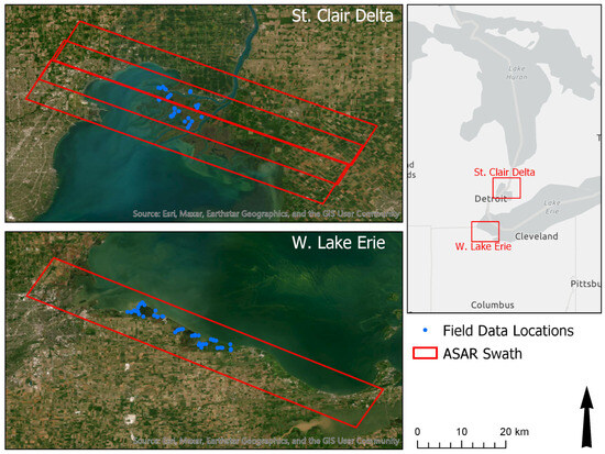
Figure 1.
Study areas within the Great Lakes Basin. Red polygons indicate ASAR swaths and blue dots indicate field locations where data were collected.
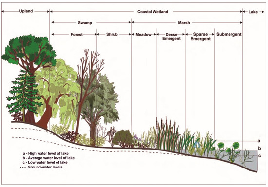
Figure 2.
Generalized zonations of coastal wetlands of the Great Lakes that form due to varying patterns of flooding and wet soils from the dry land to open water, from Wilcox et al. [31].
Throughout the past two centuries, a variety of non-native species have invaded the Great Lakes region. Some of these species are particularly aggressive and problematic. Understanding the current extent of problematic invasive species is critical for management and control, for determining areas at risk from invasion, and for assessing potential impacts on ecosystem services. One particular invasive wetland plant species, Phragmites australis, has been severely damaging to Great Lakes wetlands. Invasive Phragmites exploits rapid water level changes and quickly takes over vast areas of exposed habitat, outcompeting native species and forming dense, nearly impenetrable, tall (up to 5 m) monocultures that reduce wildlife habitat, displace native vegetation and obscure views of the lake. Coastal wetlands of the southern Great Lakes are particularly affected by invasive Phragmites as well as invasive cattail (Typha angustifolia) and a hybrid (Typha × glauca) between the native (Typha latifolia) and invasive species.
Typha, Phragmites, as well as bulrush (Schoenoplectus acutus) often form large monocultures in the coastal wetlands that are important to distinguish in mapping wetland types and for monitoring in the shifting zonations. Hereafter, we refer to these monoculture species by their genera. Since these three species form extensive areas in our study areas, much of our research is focused on them.
Typha is described as a stout stemmed emergent wetland species, often growing in dense clumps. It has broad linear leaf blades and a distinguishable brown cylindrical flowering spike. Phragmites is a perennial grass, with a stiff thin central stem and many wide leaves forming along the length of the central stem. The plumy inflorescence at the top of the stems often has a purplish hue. Schoenoplectus is a sedge known as bulrush with a thin (~1–2 cm diameter) cylindrical mainstem 1–3 m tall, typically growing in deeper water than Phragmites and Typha, up to 1.5 m [32]. However, plants as tall as 4.2 m have been found in even deeper water [33]. The only leaves are small and near the base of the plant. The inflorescence forms in a terminal panicle at the end of the stem but appears to come from the side of the stem. Schoenoplectus, Phragmites and Typha are all clonal through rhizomatous root systems and often form monocultures. There is a general trend of increasing density, height, and biomass in these species (Figure 3).
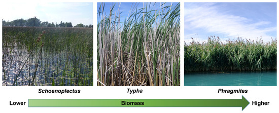
Figure 3.
Field photos of the three dominant monoculture emergent wetland types found in the lower Great Lakes, with increasing biomass from left (often sparse Schoenoplectus or bulrush) to common cattail (Typha spp.) to the invasive, often tall and dense Phragmites australis.
The two study locations are heavily diked for wetland management and, in July 2021, much of the Lake Erie wetlands inside the dikes were under a drawdown of water, leaving many with atypical low or no standing water. The St. Clair Delta had typical water level conditions for the wetland complexes.
2.2. Field Data Collection Methods
Field data were collected in support of the ASAR mission from a variety of field locations coincident to the overpasses in the St. Clair River Delta and wetlands of western Lake Erie. Field data on the extent of inundation, water levels, height, density and biomass of different wetland vegetation types, canopy closure, and other wetland characteristics were sampled to assist us in interpreting the signatures of L-, S- and C-band radar data to address our research questions. A total of 46 field sites were sampled, with 31 sites in the St. Clair delta ASAR footprint and 15 sites in the Western Lake Erie footprint (Table 1) including 9 Schoenoplectus dominated sites, 16 Phragmites dominated sites and 22 Typha dominated sites.

Table 1.
Summary of field-collected data on vegetation biomass, heights, diameters, stem densities and water depths at the St. Clair and Erie study areas. Here, we show mean values across sites by dominant species (Phragmites, Typha or Schoenoplectus) at each study area.
Field locations in the St. Clair River Delta and Western Lake Erie were visited the week of 14 July of 2021. Using 2019 base maps produced from 3 dates of Radarsat-2 PolSAR data and 3 dates of WorldView-2 imagery [5,34], we randomly selected field locations across the study area within 1 km from access points via a road or water body (via boats). Each site was at least 20 m × 20 m in size and of a fairly homogeneous ecosystem type to be commensurate with the resolution of the SAR systems and account for speckle reduction. At each site, the general wetland type was recorded (shrub, emergent, open water, upland, floating aquatic), as were the percent cover of vegetation, open water, exposed soil, and dominant and sub-dominant species present. For the monoculture sites of Phragmites, Schoenoplectus and Typha, we sub-sampled three 30 cm × 30 cm subplots that were randomly selected for measuring the number of stems by species separated by live and dead condition. Of these stems, 3 representative live individuals were measured for stem height, basal diameter, diameter at water level, and diameter at 1 m height above water along with water depth with a date/time and GPS stamp. Notes on whether vegetation was tilted from wind or fallen/knocked down were made, as well as insect damage, herbicide, or cut vegetation. As part of the protocol, GPS tagged photos were taken at each site center, in four cardinal directions, nadir and straight up. Vegetation biomass data were acquired at 27 sites in the St. Clair River Delta and 15 sites in the wetlands of western Lake Erie. Additional data were collected in wetlands without the presence of the three types of interest (Figure 1).
For biomass estimation, unpublished allometric equations were used from the University of Michigan’s database for Schoenoplectus and Typha. For Phragmites, no equations existed, so we harvested Phragmites stems from 2 locations (20 stems) and developed a new biomass equation based on height of vegetation.
Phragmites biomass, where is height in m:
Schoenoplectus biomass, where is height in cm:
Typha biomass, where is volume in cm3:
Mean height of vegetation ranged from 1.36 to 2.89 m, live biomass ranged from 16.2 to 7336.5 g/m2, and dead standing biomass from 0.0 to 9755.4 g/m2 (Table 1).
2.3. Remote Sensing Data Processing
ASAR data collected on 14 July 2021 over the Great Lakes study areas were distributed as Level 1 Single Look Complex (SLC) data and Level 2 Geocoded Amplitude Images. We downloaded Version 1.3B Level 1 and Level 2 data from NASA’s JPL website (https://uavsar.jpl.nasa.gov/cgi-bin/asar-data.pl (accessed on 23 October 2023)). Level 2 data were calibrated to Sigma Nought () intensity using the following calibration algorithm:
where represents pixel values in the provided GeoTIFFs, is the local incidence angle (provided as an ancillary dataset), is the noise bias for each polarization, and is the calibration constant. Noise bias and calibration constants were provided in associated metadata. Although the product was geocoded, there were some geolocation errors, so additional manual georeferencing was applied by visually interpreting tie points between the SAR data and high-resolution optical airphotos. For this process, we utilized USDA NAIP images collected in 2020 and 2021.
For polarimetric data analysis, we extracted SLC data from the provided HDF5 files and used PolSARpro software (v. 6.0) to apply a Refined Lee Polarimetric Filter with a 7 × 7 pixel window size to both L- and S-band data. Three polarimetric decompositions were applied to the quad polarized data. First was the van Zyl et al. [26] non-negative eigenvalue decomposition (NNED), similar to the Freeman and Durden [28] decomposition but with correction for overestimation of volume scatter, which leads to the misattribution of scattering power in the model. This model produces double-, volume and single-bounce scattering. Second was the Cloude and Pottier [35] decomposition that produces Entropy, Anisotropy and Alpha Angle parameters. H is a measure of a mix of three orthogonal scattering vectors. H = 0 implies a pure target with a single dominant scattering vector. H = 1 implies equality of all scattering vectors. Anisotropy provides the relative importance of the second and third scatters. Alpha provides the mean or dominant scattering mechanism (when H is close to 0, 0° α = single bounce, 45° α = oriented dipole, and 90° α = double bounce). Last was a decomposition specifically designed for vegetation mapping: the Neumann et al. [36] decomposition, which produces three polarimetric parameters: Delta, Tau, and Delta Phase. Moreover, ref. [36] uses a generalized volume scattering model to describe the morphological vegetation traits; the particle scattering anisotropy (Delta) and the degree of orientation randomness (Tau). The third parameter, the phase of the particle scattering anisotropy (Delta phase), is related to the particle orientation direction. Tau is an indicator of the degree of scattering randomness, similar to Cloude Pottier’s H. Georeferencing information extracted from the HDF5 files was used to geocode the polarimetric results. Like the Level 2 products, manual georeferencing was required to ensure geolocational accuracy of the output data.
For C-band Radarsat-2 (R-2), FQ10W data over Lake St. Clair and FQ62 over western Lake Erie were acquired on 26 July 2021, under a USFWS cooperative agreement. SLC data were provided for the quad-pol imagery and similar processing was performed as the L- and S-band; however, for R-2 data, both PCI and PolSARpro were used, applying radiometric terrain correction in PCI. In this case, post-processing geolocation with tie points was not necessary.
2.4. Wetland Type Mapping
Polarimetric decomposition components for S- and L-bands were used as inputs in a Random Forests [37] classifier, which has proven effective with the L-band [38]. Training and validation data for the model were derived from a combination of field data and interpretation of USDA NAIP aerial imagery. Then, 80% of training polygons were randomly selected for training and the remaining 20% were reserved as an independent validation dataset. The model was run in a Python 3.0 environment using the Sci-kit Learn package. The model was initiated with default parameters except for the number of trees, which was set to 500.
We use 2019 wetland type maps produced from multi-date high resolution digital globe worldview imagery and Radarsat-2 polarimetric data (R-2/WV) [5,34] as benchmarks to compare L- and S-band SAR-based wetland type maps in our study.
2.5. Assessment of Scattering Models
To assess the accuracy of established scattering models, we generated additional polygons representing 10 m × 10 m areas of Typha and Phragmites across a range of incidence angles from the Lake St. Clair dataset. We then extracted mean local incidence angle and the mean of each scattering type from the van Zyl NNED decomposition products to compare expected vs. observed scattering behavior.
We created co-pol phase difference histograms of the three dominant wetland monocultures, using 2019 multi-date Radarsat-2 and Worldview basemaps [5,34] to determine the extent of each across the St. Clair River Delta ASAR images. These were produced similarly to [22,23] and allow us to assess the dominant scattering type occurring via the expected co-pol phase difference (CPD). Single-bounce scatter ideally (in the absence of noise) has an expected CPD of 0°, double-bounce scattering has an expected CPD of 180°, while volume scatter has an expected uniform distribution from CPD −180° to 180°.
2.6. Assessment of Vegetation Structure Limitations
To assess how vegetation structure and biomass limited our ability to monitor inundation, we applied a thresholding method to distinguish flooded vegetation from open water and non-inundated areas. The method involves analyzing the histogram of cross-polarized backscatter to separate open water from land and flooded vegetation via Otsu-thresholding [5]. Specular reflection from water typically results in a strong bimodal distribution, so areas less than the threshold value are classified as water while areas greater than the threshold value are classified as land or flooded vegetation. The cross-polarized ratio (HH/VH or VV/VH) was used to distinguish flooded vegetation from non-flooded vegetation within areas not initially classified as water. Otsu thresholding was applied to the histogram of the cross-polarized ratio to distinguish flooded vegetation (pixels greater than the threshold value) from non-flooded vegetation (pixels less than the threshold value). In this case, we incorporated both VV/VH and HH/HV to quantify the flooded vegetation extent with pixels identified as being over the threshold value in either ratio being classified as flooded vegetation. We also assessed the relationship between total live and dead biomass and backscatter from the different frequencies and polarizations to determine which had strong relationships to biomass and whether developing biomass retrieval algorithms for wetlands in the Great Lakes was feasible.
3. Results
3.1. Wetland Type Mapping: Can L-Band and S-Band polSAR Data Be Used to Map Wetland Types with High Accuracy?
Using the backscatter and decomposition components in the Random Forests classifier, individual S-band maps had lower accuracy than the L-band maps, but a combination of the two frequencies produced the greatest accuracy (Table 2 and Table 3). The L- and S-band classification for the St. Clair Delta resulted in 92% overall accuracy, with very high accuracies for the invasive monocultures and all wetland types (>79% user’s and >73% producer’s accuracy) except for wet meadow, which was sometimes confused with agriculture (84% user’s and 46% producer’s accuracy, Table 2). The L- and S-band classification for the Western Lake Erie study area had lower overall accuracy, 76%, with comparable user’s accuracies (>85% for invasive monocultures) but significantly lower producer’s accuracies (38–82%, Table 3) than for St. Clair. We compare these results to benchmark, high-resolution SAR-optical maps previously created for these study areas [5,34] using multi-date polarimetric Radarsat-2 and Worldview imagery (R-2/WV) circa 2019. In comparison to these benchmark maps, the L- and S-band single-date map of St. Clair is comparable in terms of overall UA and PA accuracies, with improved accuracies for the three monoculture species, except PA for Schoenoplectus (Table 2). For Western Lake Erie, the L- and S-band maps are of lower accuracy than the R-2/WV 2019 maps (Table 3). Figure 4 shows the six maps generated from the S-, L-, and combined S- and L-band data for each study area. The S-band overestimates the forest and shrub and urban classes in both study areas, where there is significant confusion with the agriculture/grass class. The agriculture/grass class is also often confused with the wetland-type classes. This is especially prevalent in the L- and combined L- and S-band maps for the W. Lake Erie study area, where agriculture is a much more common land use, and many crop fields are misclassified as wet meadows. Phragmites and Typha were also occasionally incorrectly identified in crop fields in both areas, especially at the S-band. Notably, there was little confusion between Phragmites, Typha, and Schoenoplectus. Phragmites and Typha were confused with each other most often in S-band classifications, but confusion was minimal in the L-band and combined S- and L-band maps. In both areas, the most common class confused with Schoenoplectus was open water. The S- and L-band combination performed best at identifying Schoenoplectus in the St. Clair Delta but was outperformed by the L-band alone in W. Lake Erie.
Table 2.
St. Clair Delta L- and S-band map accuracy comparisons to multi-date C-band and optical basemap, R-2/WV 2019. Statistics include the overall accuracy (OA), range of User’s Accuracy (UA), range of Producer’s Accuracy (PA), and UA and PA for the dominant wetland species Phragmites (Phrag), Schoenoplectus (Schoen), Typha and combined emergent/wet meadow (Wetland).
Table 3.
Accuracy comparison for western Lake Erie map classifications with S-band, L-band and both L- and S-band, compared to the multi-date C-band and Optical basemap, R-2/WV 2019. Statistics include the overall accuracy (OA), range of User’s Accuracy (UA), range of Producer’s Accuracy (PA), and UA and PA for the dominant wetland species Phragmites (Phrag), Schoenoplectus (Schoen), Typha and combined emergent/wet meadow (Wetland).
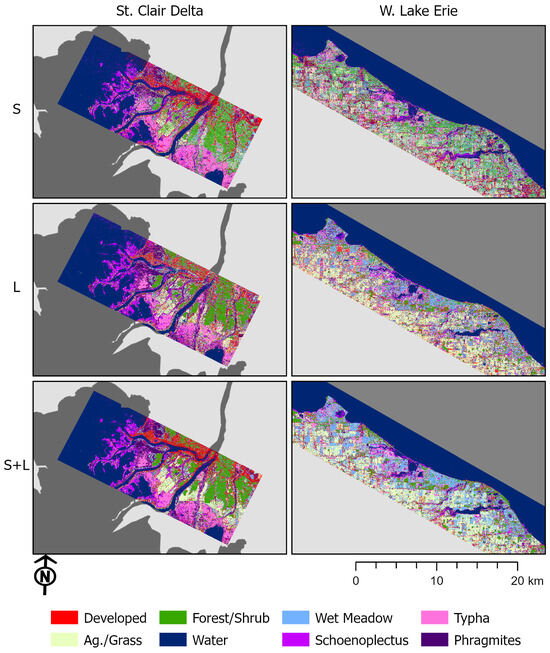
Figure 4.
Classified maps for the St. Clair Delta and W. Lake Erie study areas for S-, L-, and combined S- and L-band data.
3.2. Assessment of Scattering Models: Do Established Scattering Models Explain Polarimetric L- and S-Band SAR Interactions with Wetlands?
In an assessment of three-component decompositions [26,27,28] at the C-band, it was previously found that double-bounce scattering was mischaracterized as single bounce due to the static threshold of co-polarized phase difference in the algorithms [23,24]. The S- and L- band ASAR data have a wide range of incidence angles transitioning from 26° to 53° over a swath width of approximately 10 km. For the L-band, we found that incorrect classification of double-bounce scattering was evident, especially at shallow (large) incidence angles, with attribution as single-bounce scattering becoming noticeable at approximately 35° and becoming completely misattributed at approximately 40° (Figure 5). At the S-band, the misattribution was less pronounced across incidence angles but exhibited similar trends as the L-band data. A comparison of the Van Zyl NNED 3 component decomposition to CPD for a region of the St. Clair Delta demonstrates the variability in double bounce across the scene from near to far range (Figure 6) at each of the wavelengths. The near range is at the bottom of the images of Figure 6 and the far range is at the top. In some cases, flooded Phragmites stands (dark purple of Figure 6D) exhibited dominant volume scattering at C- and S-bands, likely due to the penetration limitations of this high biomass plant. At the L-band, double-bounce scattering (red) is dominant at steep (small) incidence angles, while single-bounce (blue) scattering dominates shallow angles of this wetland complex. For the Typha wetland types (pink of Figure 6D), the C-band (Figure 6A) showed a distinct mix of double and volume scattering as orange to yellow shades, with corresponding CPD being very dark (~−180). For the S-band, the Typha stands show mostly mixed single bounce and volume scattering (blue shades of Figure 6B) in the NNED with some mixed double bounce in the near range (red and yellow). The sparsest vegetation type, Schoenoplectus, occurs in small patches (magenta colors of Figure 6D) and is largely missed by the NNED decomposition at the L-band (Figure 6C). Only some parts of the Schoenoplectus stands are picked up by C-band and S-band NNED decompositions, despite displaying as dark and bright, respectively, in the corresponding CPD images.
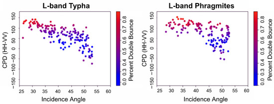
Figure 5.
Co-polarized phase difference vs. Incidence Angle for Phragmites and Typha at the L-band. The color scale indicates the percentage of double-bounce scattering from the Van Zyl NNED decomposition.
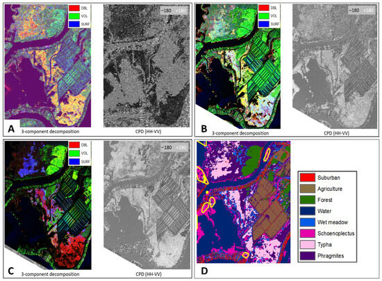
Figure 6.
St. Clair Delta false color RGB composites of the NNED 3 component (double bounce, volume scatter, single bounce) decomposition compared to the co-pol phase difference (CPD) of HH-VV for (A) C-band, (B) S-band and (C) L-band. The area shown is a subset of the St. Clair Delta study area. Incidence angle ranges from 26° to 48°, bottom to top of each image, respectively. For reference, the 2019 multi-sensor (Radarsat-2 C-band and Worldview) map (D) showing the dominant wetland types in the legend and yellow polygons indicating field polygons.
Co-Pol Phase Difference (CPD) histograms (Figure 7) were created to aid in determining dominant scattering mechanisms across the dominant wetland types. We found that, for the simpler structured cylindrical stems without leaves along the main stems, double-bounce phase difference appeared to dominate for both Typha and Schoenoplectus for the C- and S-bands, but, for the L-band, the stems of Schoenoplectus are likely too thin and sparse; thus, the expected CPD of +/−180°, indicative of double-bounce scattering, is not exhibited. However, there is a characteristic ~180° shift for Typha at L-band. For all three frequencies, surface (single-bounce) scattering is dominant for Phragmites.
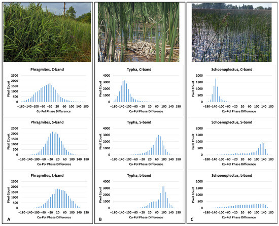
Figure 7.
Co-pol phase difference (CPD) histograms for each of the three dominant monoculture species by frequency. (A) A characteristic photo of Phragmites and the histograms for C-band (top), S-band (middle) and L-band (bottom); (B) a characteristic photo of Schoenoplectus with histograms for C-, S-, and L-band; (C) a photo of Typha followed by the histograms for C-, S- and L-bands.
3.3. Assessment of Vegetation Structure Limitations: What Are the Vegetation Structure Limitations of Different Radar Wavelengths for Wetland Inundation?
Scattering interactions with the three most common wetland genera in the lower Great Lakes, Typha, Phragmites and Schoenoplectus, varied with frequency. For Schoenoplectus, characterized by sparse, thin cylindrical spikelike stems that emerge from the water, we found that, even in dense stands, which are indicative of shallower water, L-band exhibits low backscatter at all polarizations (Figure 8); this is not much different from the open water response. However, for the shorter wavelengths of S- and C- bands, stronger responses are exhibited, particularly for the like-polarizations. Typha has a thick central stem with basal leaves spiraling upwards. Each of the three frequencies exhibits a strong but unique response from Typha, with a greater VV backscatter response at L-band over HH, and the opposite for S- and C-bands. Phragmites, which has a thin central stem with alternating leaves the full length of the stem, forms extremely dense monotypic stands in these southern Great Lakes sites. It has lower backscatter returns for all three frequencies than Typha, likely due to the high biomass, which can be less penetrable for some SAR frequencies.
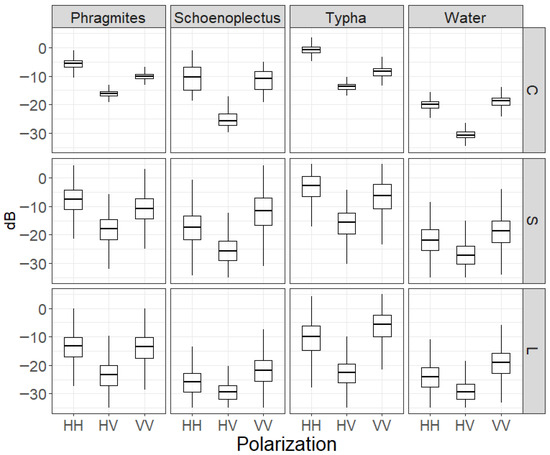
Figure 8.
Boxplots of observed backscatter from three dominant monoculture wetland types and open water for HH, HV, and VV from C-, S-, and L-band.
Inundation algorithms were applied to each frequency and showed some differences between frequencies. The L-band inundation classification produced the largest estimate of inundated area in the St. Clair Delta, followed by C-band, then S-band (Table 4). This estimate is slightly misleading, as the backscatter in S- and L-bands is significantly impacted by incidence angle effects. Far-range incidence angles over 50 degrees showed poor results, especially at L-band due to the mischaracterization of double-bounce scatter as single bounce. The S-band was less impacted by shallow incidence angles, as evidenced by the extensive classification of inundated area in St. John’s Marsh, in the northern portion of the St. Clair Delta study area (yellow of Figure 9).
Table 4.
Inundation extent in hectares for the St. Clair Delta for C-, S-, and L-bands.
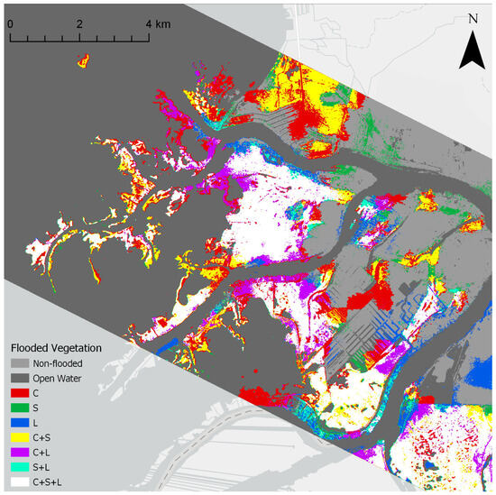
Figure 9.
Flooded vegetation extent in the St. Clair Delta as identified by each frequency. Colors show red areas as only identified by C-band, green as only identified by S-band, blue as only identified by L-band, whereas yellow was identified only by C- and S-bands, purple was identified only by C- and L-bands, cyan areas were only identified by S- and L-bands, and white areas were identified by all 3.
C-band performed best at detecting flooded Schoenoplectus. The S-band and L-band were able to detect some dense stands of Schoenoplectus but often the sparse stands were classified as open water. C-band was not able to detect flooding beneath mature Phragmites stands in many cases. The S- and L-bands had better success at detecting flooded Phragmites but were still limited in some cases, especially when mats of dead vegetation were present above the water, or where wind had blown the stalks over so the vertical structure was not as prominent. All frequencies were generally capable of detecting flooding beneath immature Phragmites, as well as monotypic stands of Typha.
When we compared inundation extent maps with field data, the S-band was slightly more accurate than the C- or L-bands, correctly assessing inundation status at 35 of 42 sites (83.3%). The C-band was able to accurately detect inundation at 34 of 42 sites (80.9%), while the L-band was correct 33 out of 42 times (78.5%).
Plots of stand biomass vs. HH backscatter by frequency (Figure 10) showed that the strongest relationship was for L-band (R2 0.71). When the non-flooded sites were added to the plots, relationships became weaker, with more outliers. For the cross polarization, the C-band had the strongest R2, and the S-band was also high but had one site with backscatter below the noise floor. These plots show that biomass influences the backscatter, with a general trend of increasing backscatter with increasing biomass. As biomass and water level vary, the dominant scattering mechanisms likely change with different frequencies.
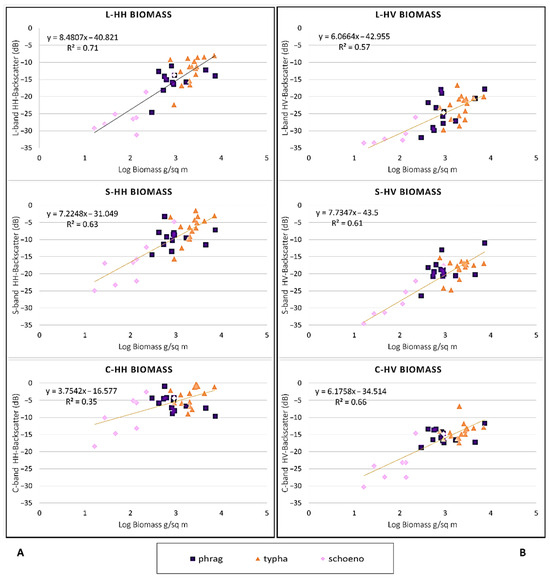
Figure 10.
Plots of (A) HH-backscatter vs. log of biomass for each frequency and (B) HV-backscatter plots for each frequency. Phragmites data are shown in purple, Typha in orange and Schoenoplectus in pink.
4. Discussion and Limitations
One of the most accurate methods of producing wetland type maps is using a combination of radar and optical multi-season data [16,39]. This allows for the capture of phenological differences in the wetland types from spring, summer and fall, as well as differences in structure and inundation conditions from radar. We found that fully polarimetric S- and L-band SAR data from a single date can be used to effectively identify the extent of various wetland plant genera and wetland types common in the southern Great Lakes without the use of other data sources, such as optical or thermal imagery. This has a significant advantage for timely mapping in locations such as the Great Lakes, which are often cloud covered. The overall accuracy of our wetland type map, created with combined L- and S- band data and machine learning classifiers, was approximately 92% for the St. Clair Delta. This is comparable to accuracy estimates achieved with combinations of three-season optical and C-band SAR imagery [5]. Other researchers have had success in mapping wetland marsh with single date C-band [19] and L- and C-band [20] polSAR decompositions using machine learning and deep learning classifiers. Fu et al. 2023 [20] found the L-band to outperform C-band and decompositions to outperform backscatter coefficients in their deep learning algorithms with the best overall accuracies of 86–88%. C-band polSAR decompositions were found to be suitable for mapping a wetland area in China where there were only two wetland types, and both had very low stature biomass herbaceous vegetation (Suaeda salsa and Spartina alterniflora) [19]. They found the C-band decompositions to allow classifications with overall accuracies of 78 to 93 percent and wetland type class accuracies between 63 and 94 percent, depending on the model.
Our results showed lower accuracies in L- and S-band SAR mapping in the Western Lake Erie study area, which is likely due to the non-flooded condition of wetlands. Many of the major wetland complexes in the region are diked with artificially manipulated water levels. During the period of the ASAR data collection, many of these Lake Erie areas had been drawn down to very low or zero water levels. This observation indicates that inundation status is a key factor in the ability to accurately identify wetland monocultures in the Great Lakes from a single date of polSAR imagery. Scattering signatures are more differentiable under flooded conditions due to double-bounce scattering from the water and vegetation. In non-flooded conditions, double-bounce scattering is greatly reduced and single-bounce or volume scatter prevails. This results in confusion with upland classes of similar vegetation structure. This is highlighted by the relatively low accuracies of non-flooded cover types in both study areas, namely, the agriculture/grass class, which was often confused with the wet meadow class. Wet meadows tend to have wet or saturated soils, but water tables mid-summer, when the ASAR were collected, are typically below the surface. Since agricultural areas are often irrigated in the Great Lakes and are also monocultures, the confusion with wet meadow is unsurprising. Similarly, the developed class had low accuracies. In the St. Clair Delta, there was often confusion between the developed class with wetland type classes, particularly Phragmites. In W. Lake Erie, the developed class was confused with several classes. This result is likely due to the large in-class variability of the area, with heavy industrial activity and urban environments in and near Toledo, and extensive low-density residential areas throughout the region that cause double bounce from the human-built structures. The high accuracies achieved for Schoenoplectus with L-band data were somewhat surprising considering the often sparse distribution of Schoenoplectus stems. It is important to note that only two sites with Schoenoplectus were visited in the W. Lake Erie study area, so additional patches were identified with the interpretation of high-resolution aerial imagery. Although the aerial imagery was collected during the same summer as the ASAR overpasses, they were not coincident, so there is a possibility that some Schoenoplectus training samples were not representative of the class and instead were more representative of open water, which would explain the confusion in the classified maps. However, double bounce from wind-drawn capillary waves could also be a cause of confusion.
Common decomposition methods are prone to misidentifying the dominant double-bounce scattering type as single-bounce scatter under certain vegetation moisture and SAR geometry conditions. Our analysis shows that this misattribution occurs at S- and L-bands, similar to previous research at the C-band [23,24]. The observed scattering behavior related to the incidence angle (Figure 5 and Figure 6) and vegetation structure (Figure 7) was generally consistent with published models of microwave scattering from dielectric cylinders [23,24]. When the anomaly will occur is a function of the radius of the vegetation stems (i.e., cylinders) relative to the wavelength [24] and the moisture in the plants. While the three-component decompositions are popular, they should be considered with caution, since we observed a lack of double bounce in the near and far ranges, depending on frequency and vegetation. It is better to use CPD without a static threshold, and a range of decomposition and backscatter information to inform inundation conditions and wetland type mapping.
Low moisture in the vegetation results in larger anomalies [24]. Using a time-series of NISAR data may allow for the monitoring of wetland plants for moisture status by using the appearance of these anomalies, such as during the onset of senescence in the fall season, or when the vegetation becomes stressed during drought or other circumstances that cause water level changes.
Our results showed that detection of flooding beneath the three dominant species that often form monocultures (Phragmites australis, Schoenoplectus acutus, and Typha spp.) was dependent on frequency in relation to the biomass and structure of the vegetation (Figure 9, Table 4). C-band, the shortest wavelength studied, performed best for detecting flooded Schoenoplectus which has the sparsest and simplest structure. L- and S-bands were able to detect flooding beneath the high-biomass, dense Phragmites canopies, whereas the C-band was limited, similar to previous findings with C- and L-bands [40]. Lamb et al. 2025 [40] found L-band backscatter thresholding to work well in mapping inundation in coastal salt marshes with varying marsh vegetation including Phragmites australis, Typha spp., Spartina and Schoenoplectus, with accuracies around 90% or better for L-HH or L-VV. They found limitations in C-VV backscatter thresholding from Sentinel-1 and suggest for C-VV data that it is best to use change detection classification from different tidal stages which produced higher accuracy (76%) maps. Radiometric modeling conducted by those authors [40] demonstrated that C-HH (as available from Radarsat-2) is more sensitive to inundation and surface changes than VV polarization (i.e., Sentinel-1). We found that all three frequencies studied (L, S, and C) were able to detect flooding beneath Typha canopies and immature Phragmites stands. Thus, a single-frequency system is going to have errors due to a mismatch of wavelength to vegetation stem size, density, height and biomass. We suggest that a combination of frequencies would be optimal for monitoring inundation extent to capture flooding beneath a range of canopy types and vegetation structures, across a range of incidence angles.
Last, for the flooded marsh wetlands, we found that we could produce a biomass retrieval algorithm from the SAR polarized data, with the strongest relationship for L-HH (R2 = 0.71), followed by C-HV (R = 0.66) and S-HH (R2 = 0.63). This is important for monitoring changes in plant biomass over a growing season and, in combination with wetland type maps, would allow for assessing wildlife habitat and nesting grounds. Furthermore, it is important for estimating C-storage in wetland vegetation and for National Greenhouse Gas Inventories [41].
It should be noted that a polarimetric signature analysis of ASAR co-pol and cross-pol channels for both L- and S-band by [42] showed that perfect behavior is exhibited by the co-pol signature, but distortions were easily identified in the cross-pol signatures. The distortions identified by [42] may impact polSAR decompositions, with either under- or overestimation of scattering elements. Since these over- or underestimations of scattering elements may be dependent on wetland cover type, it did not seem to adversely affect our ability to map wetland types. Due to the identified distortions in the cross-pol, our phase difference analysis only included the co-polarized data, which allowed us to assess dominant scattering mechanisms and relate them to the three component modeled decompositions.
There were limitations in our field data set that should be expanded for further analyses. Observations of wetland sites with non-inundated wet soil conditions were limited and should be explored further. We found that the SAR biomass retrieval algorithms had higher accuracies when the non-inundated wetlands were withheld; however, the number of non-inundated wetlands sampled was low, preventing a similar analysis for non-inundated wetland biomass retrievals. In addition, limited shrub wetlands were sampled in the field and there was a lack of samples for forested wetlands. SAR monitoring limitations in woody wetlands need to be further explored and the threshold classification technique for marsh vegetation is likely not suitable for forested wetlands; instead, a change detection approach may be necessary [40].
5. Conclusions
High-temporal-resolution multi-frequency (e.g., L-, S- and C-band) SAR dual polarization and quad polarization data will greatly improve the capabilities of mapping wetland types and monitoring hydrological conditions, regardless of cloud cover conditions during key periods of importance, e.g., during important breeding or nesting habitat seasons, which can be of very short duration. The additional knowledge gained from routine 6–12-day repeat NISAR collections will improve coastal wetland monitoring capabilities, which is of key importance as water level fluctuations and invasive species encroachment continue to alter the land–water interface. Monitoring information will be important for management decisions in areas with significant human populations, areas vital for wildlife habitat conservation or restoration and for planning for coastal resiliency. In addition, routine monitoring of wetland extent changes over time will allow for the detection of wetlands connected to the Great Lakes via surface and ground water. This is important because connectivity to the Great Lakes defines coastal wetlands, which are affected by large lake processes and regulated differently than non-coastal wetlands.
In this study, we confirmed the anomalous behavior of scattering and decompositions at the L-, S- and C-bands, which explain errors that may occur in inundation and classification mapping. Such model inaccuracies have implications for repeat-pass InSAR applications for water level changes, which requires high coherence between successive image dates. Ahern et al. [5] recommend choosing radar wavelengths that are considerably shorter, or longer, than the diameters of the wetland plant stems of interest to avoid resonance effects in double-bounce backscatter. The anomaly can appear as “holes” in the imagery due to large drops in backscatter, or changes in the dominant scattering mechanism. The plant structure (diameters, heights and density) also restricts which frequency will have penetration limitations or fail to detect vegetation presence. We analyzed three dominant genera found in the southern Great Lakes, which varied in typical size structure. While we cannot give specific thresholds for plant structure limitations with the limited dataset we observed, we provide our results with reference to the typical plant structure for the three dominant genera of our study area as a reference. For Typha, stem diameters averaged around 1.6 cm and were the largest diameters of the three dominant genera. This diameter is considerably smaller than C-, L- and S-band wavelengths, and the mean height was approximately 1.8 to 2.2 m and density 20–28 stems per sq m. This vegetation structure allowed inundation to be mapped in all three wavelengths. For Schoenoplectus, the mean stem diameter was approximately 0.80 cm, with densities of 13.8 to 195 stems per sq m and heights averaging 1.4 to 1.96 m. These wetland stands were the shortest and smallest in diameter of the three wetland genera. Inundation in Schoenoplectus was detected by C- and S-bands, but was limited at L-band, even in dense stands of Lake Erie. The stems of Schoenoplectus are too small to be detected by the L-band. For Phragmites, which differ from the other two genera in that they have central stems with leaves alternating the full length of the stem, they had mean stem diameters of 0.81 to 1.04 but were the tallest (mean 2.05 to 2.89 m) and dense (38 to 44 mean stems per sq m). Biomass was by far the greatest in the Phragmites (mean 1083 to 2667 g/sq m) and volume scatter dominated for C- and S-bands, with limited detections of inundation. Only the L-band showed dominance of double-bounce scatter in the three-component decomposition and allowed for more reliable inundation detection. For all of these genera, there are incidence angle limitations, and incidence angles shallower than 35° have higher uncertainty in inundation detection capability.
While C-band data have been routinely available from Sentinel-1 since 2015, they are limited to dual polarization (VV/VH) with penetration limitations in higher-biomass wetlands. NISAR is planned to collect quadrature polarization over the Great Lakes, allowing for the continuation of many of the methods developed in this research to be used for monitoring. S-band data will not be available over this region, but combining Sentinel-1 and or quad polarization RCM or Radarsat-2 with NISAR L-band will provide powerful tools for monitoring the wetland ecological health of the Great Lakes for the range of marsh ecosystems that exist, as well as for woody wetlands.
This study provides an advancement in understanding of polarimetric SAR for studying wetlands and understanding frequency and incidence angle limitations, as well as traditional three-component decomposition model inaccuracies. This improved understanding of SAR limitations in wetland monitoring will allow for the improved design of approaches for mapping wetland extent, wetland type, water level changes, wetland biomass and wetland contributions to carbon cycling.
Author Contributions
Conceptualization, M.J.B. and L.L.B.-C.; methodology, M.J.B. and L.L.B.-C.; software, M.J.B.; validation, M.J.B. and L.L.B.-C.; formal analysis, M.J.B. and L.L.B.-C.; investigation, M.J.B. and L.L.B.-C.; resources, M.J.B.; data curation, M.J.B.; writing—original draft preparation, L.L.B.-C.; writing—review and editing, M.J.B. and L.L.B.-C.; visualization, M.J.B.; supervision, M.J.B. and L.L.B.-C.; project administration, L.L.B.-C.; funding acquisition, L.L.B.-C. All authors have read and agreed to the published version of the manuscript.
Funding
This work was supported by NASA ISRO-ASAR Grant # 80NSSC20K0679 and USFWS Cooperative Agreement # F18AC0039 (Great Lakes Restoration Initiative (GLRI)-funded).
Data Availability Statement
Field data and map products will be made available upon request. ASAR data are available from NASA JPL https://uavsar.jpl.nasa.gov/cgi-bin/asar-data.pl (accessed on 23 October 2023). Radarsat-2 data cannot be shared publicly by the authors given restrictions in the data access agreement.
Acknowledgments
We acknowledge the field teams who assisted in collecting all of the data for this analysis, including Dorthea Vander Bilt, Karl Bosse, Charlotte Weinstein, Andrew Poley, Mary Ellen Miller, and Vanessa Barber. We thank Don Atwood for his review of the manuscript and suggested edits and Nicole Kozel for assistance in formatting and editing the text and figures.
Conflicts of Interest
The authors declare no conflicts of interest. The NASA funding agency encouraged the publication of the study results but they had no role in the design of the study; in the collection, analyses, or interpretation of data; in the writing of the manuscript; or in the final decision to publish the results.
Abbreviations
The following abbreviations are used in this manuscript:
| SAR | Synthetic Aperture Radar |
| NISAR | NASA-ISRO Synthetic Aperture Radar |
| PolSAR | Polarimetric SAR |
| CPD | Co-polarized phase difference |
| ASAR | Airborne Synthetic Aperture Radar |
| NASA | National Aeronautics and Space Administration |
| ISRO | Indian Space Research Organization |
| USFWS | United States Fish and Wildlife Service |
References
- Uzarski, D.G.; Brady, V.J.; Cooper, M.J.; Wilcox, D.A.; Albert, D.A.; Axler, R.P.; Bostwick, P.; Brown, T.N.; Ciborowski, J.J.H.; Danz, N.P.; et al. Standardized Measures of Coastal Wetland Condition: Implementation at a Laurentian Great Lakes Basin-Wide Scale. Wetlands 2017, 37, 15–32. [Google Scholar] [CrossRef]
- How the Great Lakes Coastal Wetlands are Monitored. US EPA. Available online: https://www.epa.gov/great-lakes-monitoring/how-great-lakes-coastal-wetlands-are-monitored (accessed on 6 June 2025).
- Environment Canada. Where Land Meets Water: Understanding Wetlands of the Great Lakes; Environment Canada: Gatineau, QC, Canada, 2002.
- Gronewold, A.D.; Rood, R.B. Recent Water Level Changes across Earth’s Largest Lake System and Implications for Future Variability. J. Great Lakes Res. 2019, 45, 1–3. [Google Scholar] [CrossRef]
- Battaglia, M.J.; Banks, S.; Behnamian, A.; Bourgeau-Chavez, L.; Brisco, B.; Corcoran, J.; Chen, Z.; Huberty, B.; Klassen, J.; Knight, J.; et al. Multi-Source EO for Dynamic Wetland Mapping and Monitoring in the Great Lakes Basin. Remote Sens. 2021, 13, 599. [Google Scholar] [CrossRef]
- Samadzadegan, F.; Toosi, A.; Dadrass Javan, F. A critical review on multi-sensor and multi-platform remote sensing data fusion approaches: Current status and prospects. Int. J. Remote Sens. 2025, 46, 1327–1402. [Google Scholar] [CrossRef]
- Gallant, A. The Challenges of Remote Monitoring of Wetlands. Remote Sens. 2015, 7, 10938–10950. [Google Scholar] [CrossRef]
- Mahdavi, S.; Salehi, B.; Granger, J.; Amani, M.; Brisco, B.; Huang, W. Remote Sensing for Wetland Classification: A Comprehensive Review. GISci. Remote Sens. 2017, 55, 623–658. [Google Scholar] [CrossRef]
- DeLancey, E.R.; Simms, J.F.; Mahdianpari, M.; Brisco, B.; Mahoney, C.; Kariyeva, J. Comparing Deep Learning and Shallow Learning for Large-Scale Wetland Classification in Alberta, Canada. Remote Sens. 2019, 12, 2. [Google Scholar] [CrossRef]
- Abdelmajeed, A.Y.; Albert-Saiz, M.; Rastogi, A.; Juszczak, R. Cloud-based remote sensing for wetland monitoring—A review. Remote Sens. 2023, 15, 1660. [Google Scholar] [CrossRef]
- Merchant, M.A. Classifying Open Water Features Using Optical Satellite Imagery and an Object-Oriented Convolutional Neural Network. Remote Sens. Lett. 2020, 11, 1127–1136. [Google Scholar] [CrossRef]
- Chen, Z.; White, L.; Banks, S.; Behnamian, A.; Montpetit, B.; Pasher, J.; Duffe, J.; Bernard, D. Characterizing Marsh Wetlands in the Great Lakes Basin with C-Band InSAR Observations. Remote Sens. Environ. 2020, 242, 111750. [Google Scholar] [CrossRef]
- Canisius, F.; Brisco, B.; Murnaghan, K.; van der Kooij, M.; Keizer, E. SAR Backscatter and InSAR Coherence for Monitoring Wetland Extent, Flood Pulse and Vegetation: A Study of the Amazon Lowland. Remote Sens. 2019, 11, 720. [Google Scholar] [CrossRef]
- Banks, S.N.; Behnamian, A.; Chu, K.C.K.; Hamilton, R.; Duffe, J.; Pasher, J. Demonstrating How FPCA Can Leverage SAR Time-Series Information to Distinguish Wetlands and Uplands Based on Seasonal Backscatter Trends. IEEE J. Sel. Top. Appl. Earth Obs. Remote Sens. 2025, 18, 14416–14437. [Google Scholar] [CrossRef]
- Bourgeau-Chavez, L.L.; Endres, S.L.; Graham, J.A.; Hribljan, J.A.; Chimner, R.A.; Lillieskov, E.A.; Battaglia, M.J. Mapping Peatlands in Boreal and Tropical Ecoregions. Compr. Remote Sens. 2018, 6, 24–44. [Google Scholar] [CrossRef]
- Bourgeau-Chavez, L.; Endres, S.; Battaglia, M.; Miller, M.; Banda, E.; Laubach, Z.; Higman, P.; Chow-Fraser, P.; Marcaccio, J. Development of a Bi-National Great Lakes Coastal Wetland and Land Use Map Using Three-Season PALSAR and Landsat Imagery. Remote Sens. 2015, 7, 8655–8682. [Google Scholar] [CrossRef]
- Brisco, B.; Kapfer, M.; Hirose, T.; Tedford, B.; Liu, J.B. Evaluation of C-Band Polarization Diversity and Polarimetry for Wetland Mapping. Can. J. Remote Sens. 2011, 37, 82–92. [Google Scholar] [CrossRef]
- Touzi, R.; Deschamps, A.; Rother, G. Wetland Characterization Using Polarimetric RADARSAT-2 Capability. Can. J. Remote Sens. 2007, 33 (Suppl. S1), S56–S67. [Google Scholar] [CrossRef]
- Zhang, X.; Xu, J.; Chen, Y.; Xu, K.; Wang, D. Coastal Wetland Classification with GF-3 Polarimetric SAR Imagery by Using Object-Oriented Random Forest Algorithm. Sensors 2021, 21, 3395. [Google Scholar] [CrossRef] [PubMed]
- Fu, B.; Li, H.; Liu, M.; Yao, H.; Gao, E.; Sun, W.; Zhang, S.; Fan, D. Performance Evaluation of Backscattering Coefficients and Polarimetric Decomposition Parameters for Marsh Vegetation Mapping Using Multi-Sensor and Multi-Frequency SAR Images. Ecol. Indic. 2023, 157, 111246. [Google Scholar] [CrossRef]
- Huang, W.; DeVries, B.; Huang, C.; Lang, M.; Jones, J.; Creed, I.; Carroll, M. Automated Extraction of Surface Water Extent from Sentinel-1 Data. Remote Sens. 2018, 10, 797. [Google Scholar] [CrossRef]
- Atwood, D.; Battaglia, M.; Bourgeau-Chavez, L.; Ahern, F.; Murnaghan, K.; Brisco, B. Exploring Polarimetric Phase of Microwave Backscatter from Typha Wetlands. Can. J. Remote Sens. 2020, 46, 49–66. [Google Scholar] [CrossRef]
- Ahern, F.J.; Brisco, B.; Battaglia, M.J.; Bourgeau-Chavez, L.; Atwood, D.; Murnaghan, K. SAR Polarimetric Phase Differences in Wetlands: Information and Mis-Information. Can. J. Remote Sens. 2022, 48, 703–721. [Google Scholar] [CrossRef]
- Ahern, F.; Brisco, B.; Murnaghan, K.; Lancaster, P.; Atwood, D.K. Insights into Polarimetric Processing for Wetlands from Backscatter Modeling and Multi-Incidence Radarsat-2 Data. IEEE J. Sel. Top. Appl. Earth Obs. Remote Sens. 2018, 11, 3040–3050. [Google Scholar] [CrossRef]
- Hong, S.-H.; Wdowinski, S. Double-Bounce Component in Cross-Polarimetric SAR from a New Scattering Target Decomposition. IEEE Trans. Geosci. Remote Sens. 2013, 52, 3039–3051. [Google Scholar] [CrossRef]
- van Zyl, J.; Arii, M.; Kim, Y. Model-Based Decomposition of Polarimetric SAR Covariance Matrices Constrained for Nonnegative Eigenvalues. IEEE Trans. Geosci. Remote Sens. 2011, 49, 3452–3459. [Google Scholar] [CrossRef]
- Freeman, A.; Durden, S.L. A Three-Component Scattering Model for Polarimetric SAR Data. IEEE Trans. Geosci. Remote Sens. 1998, 36, 963–973. [Google Scholar] [CrossRef]
- Yamaguchi, Y.; Moriyama, T.; Ishido, M.; Yamada, H. Four-Component Scattering Model for Polarimetric SAR Image Decomposition. IEEE Trans. Geosci. Remote Sens. 2005, 43, 1699–1706. [Google Scholar] [CrossRef]
- Siqueira, P. L- and S-Band Polarimetric Data Collections by ISRO’s ASAR Instrument in Support of NISAR Ecosystems Algorithm Development. In Proceedings of the IGARSS 2022–2022 IEEE International Geoscience and Remote Sensing Symposium, Kuala Lumpur, Malaysia, 17–22 July 2022; pp. 7468–7470. [Google Scholar] [CrossRef]
- Albert, D.A. Between Land and Lake: Michigan’s Great Lakes Coastal Wetlands; Michigan Natural Features Inventory: Lansing, MI, USA, 2003. [Google Scholar]
- Wilcox, D.A.; Thompson, T.A.; Booth, R.K.; Nicholas, J.R. Lake-Level Variability and Water Availability in the Great Lakes; Circular 1311; U.S. Geological Survey: Reston, VA, USA, 2007. Available online: https://pubs.usgs.gov/circ/2007/1311/pdf/circ1311_web.pdf (accessed on 26 January 2024).
- Tilley, D. Plant Guide for Hardstem Bulrush (Schoenoplectus acutus); SDA-Natural Resources Conservation Service; Idaho Plant Materials Center: Aberdeen, UK, 2012.
- Reznicek, A.A.; Voss, E.G.; Walters, B.S. University of Michigan. Available online: https://michiganflora.net/genus/schoenoplectus (accessed on 26 January 2024).
- Bourgeau-Chavez, L.L.; Graham, J.; Battaglia, M.J.; White, L.; Klassen, J.; Vander Bilt, D.L.; Poley, A.F.; Pelletier, K.; Brisco, B.; Huberty, B. Great Lakes Remote Sensing ESRI Storymap, High Resolution Monitoring of Coastal Great Lakes Wetlands in 4D. 2021. Available online: https://mtu.maps.arcgis.com/apps/MapSeries/index.html?appid=2d06583e97844ea892413e2290cbe885 (accessed on 6 June 2025).
- Cloude, S.R.; Pottier, E. An Entropy Based Classification Scheme for Land Applications of Polarimetric SAR. IEEE Trans. Geosci. Remote Sens. 1997, 35, 68–78. [Google Scholar] [CrossRef]
- Neumann, M.; Ferro-Famil, L.; Jager, M.; Reigber, A.; Pottier, E. A Polarimetric Vegetation Model to Retrieve Particle and Orientation Distribution Characteristics; HAL (Le Centre pour la Communication Scientifique Directe). In Proceedings of the 2009 IEEE International Geoscience and Remote Sensing Symposium, Cape Town, South Africa, 12–17 July 2009. [Google Scholar] [CrossRef]
- Breiman, L. Random Forests. Mach. Learn. 2001, 45, 5–32. [Google Scholar] [CrossRef]
- Adeli, S.; Salehi, B.; Mahdianpari, M.; Quackenbush, L.J.; Chapman, B. Moving toward L—Band NASA—ISRO SAR Mission (NISAR) Dense Time Series: Multipolarization Object—Based Classification of Wetlands Using Two Machine Learning Algorithms. Earth Space Sci. 2021, 8, e2021EA001742. [Google Scholar] [CrossRef]
- Mahdianpari, M.; Granger, J.E.; Mohammadimanesh, F.; Salehi, B.; Brisco, B.; Homayouni, S.; Gill, E.; Huberty, B.; Lang, M. Meta-Analysis of Wetland Classification Using Remote Sensing: A Systematic Review of a 40-Year Trend in North America. Remote Sens. 2020, 12, 1882. [Google Scholar] [CrossRef]
- Lamb, B.T.; McDonald, K.C.; Tzortziou, M.A.; Tesser, D.S. Characterizing Tidal Marsh Inundation with Synthetic Aperture Radar, Radiometric Modeling, and in Situ Water Level Observations. Remote Sens. 2025, 17, 263. [Google Scholar] [CrossRef]
- Byrd, K.B.; Ballanti, L.; Thomas, N.; Nguyen, D.; Holmquist, J.R.; Simard, M.; Windham-Myers, L. A Remote Sensing-Based Model of Tidal Marsh Aboveground Carbon Stocks for the Conterminous United States. ISPRS J. Photogramm. Remote Sens. 2018, 139, 255–271. [Google Scholar] [CrossRef]
- Kumar, S. Polarimetric Distortion Analysis of L- and S-Band Airborne SAR (LS-ASAR): A Precursor Study of the Spaceborne Dual-Frequency L- and S-Band NASA ISRO Synthetic Aperture Radar (NISAR) Mission. Eng. Proc. 2022, 21, 77. [Google Scholar] [CrossRef]


Disclaimer/Publisher’s Note: The statements, opinions and data contained in all publications are solely those of the individual author(s) and contributor(s) and not of MDPI and/or the editor(s). MDPI and/or the editor(s) disclaim responsibility for any injury to people or property resulting from any ideas, methods, instructions or products referred to in the content. |
© 2025 by the authors. Licensee MDPI, Basel, Switzerland. This article is an open access article distributed under the terms and conditions of the Creative Commons Attribution (CC BY) license (https://creativecommons.org/licenses/by/4.0/).