A Hierarchical Absolute Visual Localization System for Low-Altitude Drones in GNSS-Denied Environments

Highlights

What are the main findings?

• A hierarchical visual localization framework is proposed that integrates coarse-to-fine positioning through image retrieval, image registration, IMU-based correction, and sliding-window map updates, effectively addressing drift and initialization dependency issues in GNSS-denied environments for UAV localization.
• By adapting the DINOv2 model and improving SuperPoint keypoint detection, the robustness of image retrieval in complex environments and the real-time performance and accuracy of image registration are significantly enhanced.

What is the implication of the main finding?

• This work provides a high-precision, GNSS-free autonomous localization solution for low-altitude UAVs in satellite-denied environments, offering substantial value for enhancing navigation capabilities under complex conditions.
• The proposed technique shows broad application potential in scenarios requiring high-precision positioning with unreliable satellite signals, such as environmental monitoring, precision agriculture, and emergency rescue operations.

Abstract

Current drone navigation systems primarily rely on Global Navigation Satellite Systems (GNSSs), but their signals are susceptible to interference, spoofing, or suppression in complex environments, leading to degraded positioning performance or even failure. To enhance the positioning accuracy and robustness of low-altitude drones in satellite-denied environments, this paper investigates an absolute visual localization solution. This method achieves precise localization by matching real-time images with reference images that have absolute position information. To address the issue of insufficient feature generalization capability due to the complex and variable nature of ground scenes, a visual-based image retrieval algorithm is proposed, which utilizes a fusion of shallow spatial features and deep semantic features, combined with generalized average pooling to enhance feature representation capabilities. To tackle the registration errors caused by differences in perspective and scale between images, an image registration algorithm based on cyclic consistency matching is designed, incorporating a reprojection error loss function, a multi-scale feature fusion mechanism, and a structural reparameterization strategy to improve matching accuracy and inference efficiency. Based on the above methods, a hierarchical absolute visual localization system is constructed, achieving coarse localization through image retrieval and fine localization through image registration, while also integrating IMU prior correction and a sliding window update strategy to mitigate the effects of scale and rotation differences. The system is implemented on the ROS platform and experimentally validated in a real-world environment. The results show that the localization success rates for the h, s, v, and w trajectories are 95.02%, 64.50%, 64.84%, and 91.09%, respectively. Compared to similar algorithms, it demonstrates higher accuracy and better adaptability to complex scenarios. These results indicate that the proposed technology can achieve high-precision and robust absolute visual localization without the need for initial conditions, highlighting its potential for application in GNSS-denied environments.

1. Introduction

In recent years, unmanned aerial vehicles (UAVs) have been widely applied in both military and civilian domains, including intelligence reconnaissance, military strikes, environmental monitoring, precision agriculture, search and rescue, and logistics delivery, due to their high mobility and autonomy. Autonomous UAV systems are capable of performing various tasks such as path planning, target detection, and target tracking, all of which rely on accurate positioning and navigation technologies.

Currently, UAV positioning and navigation primarily depend on the Global Navigation Satellite System (GNSS). Since GNSS positioning is based on the precise measurement of radio signal propagation time, any obstacles between the UAV and the signal-transmitting satellites can interfere with signal transmission. In complex environments such as urban canyons, mountainous terrain, dense urban areas, or regions with strong electromagnetic interference, the quality of GNSS signal reception can be severely degraded, potentially resulting in complete positioning failure. Moreover, GNSS systems are highly susceptible to intentional disruptions, including jamming (high-power noise signals that disrupt normal signal reception) and spoofing (deceptive signals that simulate pseudo-satellites to mislead the receiver into calculating incorrect positions), which pose significant threats to positioning accuracy. In recent regional conflicts, GNSS spoofing has been used to undermine the navigation performance of UAVs and precision-guided weapons, underscoring the critical importance of developing positioning and navigation technologies that are resilient in satellite-denied environments.

To address the issue of short-term GNSS signal loss, an Inertial Navigation System (INS) can be introduced as a supplementary solution. This system calculates motion parameters such as velocity and attitude by utilizing data from internal sensors like gyroscopes and accelerometers, thereby enabling navigation. However, during extended UAV flights, INS suffers from drift errors caused by sensor imperfections, error accumulation through integration, and variations in external environmental conditions. This results in a growing discrepancy between the estimated and actual positions over time. In the absence of GNSS signals to correct absolute positions, the navigation system may eventually diverge and even fail entirely. Therefore, it is imperative to develop a positioning technology capable of providing the absolute position of UAVs without relying on GNSS.

In recent years, advancements in computer vision have significantly driven the development of UAV visual localization technologies. UAV visual localization refers to the process in which visual sensors mounted on UAVs capture images of the environment, and onboard computers process this visual data—often in combination with prior position information and Inertial Measurement Unit (IMU) data—to estimate the pose of the UAV in real time. This approach offers several advantages, including low power consumption, low cost, high efficiency, and strong resistance to interference. Currently, vision-based UAV localization and navigation techniques can be broadly categorized into two types: relative visual localization (RVL) and absolute visual localization (AVL).

Relative visual localization includes visual odometry (VO) and Simultaneous Localization and Mapping (SLAM). VO can only estimate the UAV pose relative to the initial frame, and thus cannot determine the global position of the UAV. Visual SLAM has been widely applied and achieved good performance in indoor environments [1] and ultra-low-altitude outdoor scenarios [2]. However, when applied to aerial–ground scenarios during UAV outdoor flight, visual SLAM systems tend to degrade rapidly due to the difficulty of achieving loop closure over the large-scale mapping area. In summary, relative visual localization methods are inherently dependent on previous estimations and are prone to cumulative errors, which cannot be eliminated without access to global absolute position updates.

In contrast, absolute visual localization methods can overcome the aforementioned limitations. These methods typically perform localization by matching real-time UAV images with pre-stored satellite reference maps. The key advantages are that they are immune to external signal interference, free from cumulative errors, and produce independent localization results for each frame, thus eliminating the need for loop closure. The global position obtained via absolute visual localization can effectively correct the drift error accumulated by INS during long-term operation and serves as a robust supplement in the event of GNSS signal loss. This is critical for enabling accurate localization and navigation of UAVs in complex satellite-denied environments.

However, due to the complexity of such environments and the inherent differences between UAV-acquired images and satellite imagery, several challenges arise:

(1)

Complex and diverse ground environments. Ground scenes are influenced by numerous factors. Lighting conditions can cause overexposure or underexposure, affecting image quality. Terrain undulations and landform variations increase texture complexity. Seasonal changes can alter color and contrast, particularly in vegetation-covered areas. These factors place high demands on the robustness and generalization capabilities of visual algorithms.

(2)

Significant differences in altitude and viewing angle between UAV images and satellite images. Satellite imagery is captured from high altitudes, offering broad coverage but lower resolution. UAVs, on the other hand, fly at low altitudes and can capture finer ground details. Moreover, satellites typically capture images in a nadir (top–down) view, whereas UAVs can flexibly adjust their camera angles to capture multi-perspective views. These differences introduce substantial variations in image scale and viewpoint.

This paper focuses on navigation and positioning of low-altitude unmanned aerial vehicles (UAVs) in typical satellite-denied environments. It centers around image retrieval-based and image registration-based localization methods, and further builds a hierarchical absolute visual localization framework based on these two approaches. An absolute visual localization technique suitable for satellite-denied environments is proposed, which significantly improves the positioning accuracy and robustness of UAVs, offering substantial theoretical significance and practical application value. The main contributions of this paper are as follows:

(1)

A hierarchical framework for absolute visual localization. To address the limitations of existing image retrieval and image registration methods, we propose an integrated hierarchical strategy that operates from coarse to fine. During system initialization, image retrieval is employed to estimate a coarse location, followed by image registration within a local sub-map to achieve fine-grained localization. Furthermore, IMU-based real-time image correction and a sliding-window map update strategy are incorporated, effectively mitigating the drift and initialization dependency issues inherent to single-method approaches. This hierarchical framework constitutes the core innovation of this work.

(2)

Adapting visual foundation models for enhanced retrieval robustness. We investigate the applicability of the DINOv2 model to absolute visual localization for UAVs, analyzing and comparing the effects of different network depths and feature selection strategies. In addition, unsupervised feature aggregation methods such as GeM are integrated to strengthen global representations, thereby achieving more reliable image retrieval in complex environments.

(3)

Improved keypoint detection for real-time performance and consistency. In the image registration module, structural re-parameterization is introduced into the encoder of SuperPoint, which significantly accelerates inference while preserving feature extraction consistency. Moreover, the combination of cycle-consistency matching and multi-scale feature fusion enhances matching accuracy under challenging conditions involving scale and viewpoint variations.

2. Related Work

With the increasing occurrence of GNSS-denied scenarios, the navigation and positioning technologies for unmanned aerial vehicles (UAVs) are facing new challenges, and the demand for absolute visual localization is becoming more urgent.

Early research primarily focused on terrain contour matching techniques using Digital Orthophoto Maps (DOMs) and Digital Elevation Models (DEMs) [3]. These methods rely on known terrain information and offer high stability against variations in lighting and seasons. However, preparing DOMs or DEMs is typically more complex than preparing digital satellite maps and requires substantial storage space. Moreover, terrain contour matching techniques are not well-suited for flat regions with minimal elevation variation.

With the advancement of computer vision technologies, Visual Geo-localization (VG) methods have emerged as alternative solutions for achieving absolute visual localization. These methods compare real-time UAV images with pre-stored satellite imagery to determine location [4]. Currently, VG methods can be broadly categorized into two main approaches: image retrieval-based and image registration-based localization. The following sections will elaborate on the current research status of these two categories.

Image retrieval-based methods, also known as place recognition (PR) or Visual Place Recognition (VPR), aim to estimate the approximate geographical location of a query image by retrieving the most similar image from a geo-tagged database. In these methods, global descriptors are typically used to represent both the query image and the tile images of satellite maps.

Traditional global descriptors are often generated by aggregating local descriptors, such as Bag of Words (BoW), Fisher Vectors (FVs), and Vectors of Locally Aggregated Descriptors (VLADs). These techniques are usually combined with hand-crafted local features such as SIFT and HOG [5,6]. In recent years, image retrieval methods based on convolutional neural networks (CNNs) and Transformers have also been proposed [7,8,9]. However, early mainstream VPR datasets mainly focus on ground-level perspectives, such as images captured by pedestrians or vehicles in indoor or urban environments. Representative datasets in this area include Pitts30k [7], Oxford5K [10], Mapillary Street-Level Sequences (MSLS) [11], and GSV-Cities [12].

In recent years, with the growing affordability and widespread use of UAVs, increasing attention has been paid to localization tasks from aerial viewpoints. Datasets such as CVUSA [13] and VIGOR [14] are designed for satellite-to-ground image matching tasks. The Where-CNN proposed by Lin et al. [15] was the first to combine CNN models with a Siamese neural network architecture for satellite-to-ground image matching. CVM-Net, proposed by Hu et al. [16], integrates NetVLAD with a Siamese network to enhance feature extraction quality and introduces a weighted soft-margin ranking loss function, which accelerates convergence and improves accuracy. However, the above methods mainly target satellite-to-ground matching tasks. Satellite images are typically orthophotos, while UAV images often involve significant viewpoint variations, including differences in height and angle, making the matching task more challenging.

Currently, publicly available datasets that include UAV perspectives are relatively limited, and the organization and structure of these datasets vary significantly, which restricts the broader application of image retrieval-based localization methods as shown in

Table 1. Summary of UAV visual localization datasets.

Dataset Name	Scale	Coverage Area	Viewpoint Type
University-1652 [17,18]	50.2 k	72 universities, 1652 buildings	Satellite-UAV-Ground
SUE-200 [18]	6.1 k	1 university in Shanghai, China	Satellite-UAV
DenseUAV [19]	20.3 k	14 universities in Zhejiang, China	Satellite-UAV
VPAir [20]	5.4 k	University of Bonn, Germany	Satellite-UAV
ALTO [21]	15 k	From Ohio to Pittsburgh, USA	Satellite-UAV

.

Wang et al. [22] proposed the Local Pattern Network (LPN), which introduces a circular partitioning strategy to fully exploit the contextual information of adjacent regions in images, thereby enriching the discriminative information for cross-view matching. This module also exhibits good adaptability to rotational variations and can be easily integrated into other networks. Dai et al. [23] introduced a Transformer-based backbone network, which partitions image feature maps according to their heat distribution and aligns multiple regions across different views. Additionally, the paper proposed a multi-sampling strategy to address the significant imbalance between the quantity of satellite images and other types of images. Keetha et al. [24] were the first to utilize large-scale pre-trained visual foundation models to achieve universal place recognition under any environment, any time, and any viewpoint. This work demonstrated the powerful potential of visual foundation models in the field of place recognition, though it did not delve deeply into UAV visual navigation applications.

Most current algorithms heavily rely on supervised training approaches and are typically trained on a single dataset. While this practice can yield satisfactory performance under specific conditions, it limits the models’ generalization ability in open-world scenarios, making them less effective in adapting to complex ground environments.

The image registration-based methods first establish an initial position for the UAV and then perform registration between the real-time images of the UAV and reference satellite images. Image registration methods can be broadly categorized into three types: template matching, hand-crafted feature point matching, and deep learning-based image matching.

Template matching methods generally adopt gray-level-based image registration techniques, constructing similarity measures based on pixel intensities between images. Then, appropriate search strategies are used to determine the transformation relationship between the two images at the extrema of the similarity measure. Common methods include Normalized Cross-Correlation (NCC) [25] and Mutual Information (MI) [26,27]. However, such methods are sensitive to weather, illumination, noise, and other factors, which undermines their localization accuracy and robustness. In addition, with the increase in image resolution, these methods require the traversal of all pixel intensities, leading to an exponential increase in computational complexity.

SIFT [28], SURF [29], and ORB [30] are widely used hand-crafted feature point matching algorithms, among which ORB has the highest computational efficiency and is suitable for real-time applications. An evaluation framework proposed by Couturieri et al. demonstrated that the ORB algorithm achieved the lowest localization error over a 4 km trajectory. Nevertheless, traditional feature extraction methods still suffer significant performance degradation in challenging scenarios such as low-texture regions, occlusions, and illumination changes, limiting the accuracy of UAV localization.

In recent years, with the development of deep learning, image registration methods based on CNNs and Transformers have emerged, showing superior performance compared to traditional methods. LIFT [31] was the first to unify keypoint detection, orientation estimation, and descriptor extraction, but it relies heavily on large amounts of labeled data. SuperPoint [32] proposed a self-supervised training framework that balances efficiency and accuracy, making it suitable for real-world applications. LofTR [33] achieved sub-pixel-level semi-dense matching and performed well in low-texture regions, albeit at a high computational cost. SuperGlue [34] and LightGlue [35] leverage graph neural networks and adaptive strategies to enhance matching accuracy and efficiency, offering greater robustness in complex environments. Meanwhile, deep learning methods have also been explored for cross-domain tasks. For instance, ref. [36] employed convolutional neural networks (CNNs) together with unsupervised domain adaptation for crater detection and registration in planetary exploration missions, further demonstrating the potential of deep models in terrain recognition.

For localization tasks based on deep learning image matching algorithms, the current existing methods are as follows. Gorofth et al. [37] proposed a localization approach that combines CNN and visual odometry (VO). The method consists of two identical CNN networks, where the aligned images are passed through the two networks respectively, followed by an Inverse Compositional Lucas-Kanade (ICLK) layer to enable backpropagation. The position of the UAV can be directly derived from the homography matrix output by the CNNs in combination with VO. Kinnari et al. [38] proposed a localization method that integrates Visual-Inertial Odometry (VIO) and Monte Carlo localization. This approach relies on a local planar assumption and requires orthorectification of UAV images but does not require the camera to be strictly downward-facing. Mao et al. [39] proposed a method that combines Visual-Inertial Odometry (VIO) with 2D georeferenced maps. This approach registers the 3D points reconstructed by VIO with a 2D map and fuses the results through graph optimization, achieving smooth and drift-free localization. Recently, ref. [40] introduced a visual localization system that integrates image matching, visual odometry, and terrain-weighted constraint optimization. This method acquires precise virtual control points through bidirectional feature matching and incorporates terrain weights into the sliding-window optimization to mitigate drift errors, demonstrating high robustness in complex environments such as plains, hills, and urban areas. Gurgu et al. [41] were the first to achieve absolute visual localization without GNSS by using a deep learning-based feature point extraction algorithm. The authors adopted the SuperPoint + SuperGlue method for feature extraction and matching, and used free, open-source satellite imagery from Google Earth as the reference map. Li et al. [42] proposed a multimodal image registration method based on decoupled representations to address the modality differences between visible and near-infrared images. This method embeds images of different modalities into a unified shape feature space, introduces intensity loss constraints, and directly predicts affine transformation parameters, enabling efficient and accurate UAV localization even in night-time and adverse weather conditions. Chen et al. [43] designed a feature matching network that encodes rotation invariance to obtain sparse local features that are robust to rotation and viewpoint changes. The authors also proposed a local-to-global feature matching strategy that adaptively selects high-quality matching point pairs. Due to the lack of publicly available code and benchmark datasets for current localization systems, it is difficult to conduct comparative analyses among different systems. This paper summarizes the experimental setups and results of several other localization methods, as shown in

Table 2. Summary of current localization methods.

Author	Year	Method	Experimental Setup	Accuracy
Chen et al. [43]	2024	Image registration + PNP	Flight altitude: 169–325 m Flight distance: 0.85–1.76 km	8 m
He et al. [44]	2023	Image retrieval + VO	Flight altitude: 50–100 m Flight distance: 0.88–1 km	19 m
Gurgu et al. [41]	2022	Image registration	Flight altitude: 120 m Flight distance: 1.2 km	16 m
Kinnari et al. [38]	2021	Image registration + VIO	Flight altitude: 92 m Flight distance: 4.0–6.8 km	17 m
Hou et al. [45]	2020	Image registration + PNP + BA optimization	Flight altitude: 500 m Flight distance: 0.54–0.75 km	14 m
Goforth et al. [37]	2019	Image registration + VO	Flight altitude: 200 m Flight distance: 0.85 km	25 m

, where PnP stands for Perspective-n-Point, BA denotes Bundle Adjustment, VO represents visual odometry, and VIO stands for Visual-Inertial Odometry.

The current state of research can be summarized as follows:

(1)

Image retrieval-based methods exhibit a certain level of robustness and can adapt to variations in lighting, viewpoints, and seasonal changes, making them suitable for rapid matching in large-scale scenes. However, they cannot provide precise location information and typically rely on pre-constructed databases, which limits their ability to meet real-time processing requirements. In continuous frame applications, due to the lack of temporal and spatial constraints, their stability and accuracy are relatively poor.

(2)

Image registration-based methods can achieve pixel-level alignment and offer high localization accuracy. However, they often assume that the initial position of the UAV is known or that the camera is downward-facing—conditions that are difficult to satisfy in practice. Furthermore, in the absence of initial position information, searching high-dimensional features is time-consuming and memory-intensive, which affects efficiency. Therefore, this method is more suitable for precise localization in continuous scenes but requires other approaches to provide initial positioning.

In summary, image retrieval methods are suitable for fast matching, while image registration methods excel in high-precision alignment. Each has its own advantages and limitations, and they can complement each other. Combining the two is expected to significantly enhance the accuracy and efficiency of UAV visual localization and will be the focus of subsequent research in this paper.

3. Method

Image retrieval-based localization methods are suitable for rapidly selecting reference images similar to the real-time image in large-scale scenes. However, in continuous frame localization, these methods lack temporal and spatial constraints and thus cannot provide precise positional information. In contrast, image registration-based localization methods can achieve pixel-level accurate alignment, but they require initial position information as a prerequisite—something image retrieval-based methods can conveniently provide.

Both methods have certain limitations and lack effective integration, which prevents them from fully leveraging their respective strengths in practical applications. To address this issue, this paper proposes a hierarchical localization system that performs coarse-to-fine localization as illustrated in Figure 1. Based on the image retrieval method, the system determines the approximate location of the UAV during initialization, thereby narrowing the reference image search space and completing coarse matching. If image retrieval fails, the system repeats the retrieval process until success. After initialization, subsequent frames no longer perform global retrieval; instead, image registration and fine-grained localization are carried out within the constrained sub-map defined by the previous frame result. The temporal constraint is reflected in using the pose of the previous frame as a prior for the next registration, while the spatial constraint is enforced by dynamically updating the sub-map within a sliding window, thereby narrowing the search range and improving both efficiency and robustness. Subsequently, it employs image registration-based localization, incorporating a real-time image correction strategy based on IMU prior information and a reference sub-image update strategy based on a sliding window to achieve fine localization in the continuous frame sequence. Finally, map updates and pose estimation are performed to obtain the localization information of the UAV.

3.1. Image Retrieval Algorithm Based on Visual Backbone Model

Although image retrieval-based localization methods can quickly retrieve the approximate location of the UAV in large-scale scenes, there are still several issues with these methods.

First, the feature generalization ability is weak. Current supervised learning algorithms have achieved good results on publicly available UAV visual localization datasets. However, UAVs face various complex environmental conditions during actual flight. Models trained only on these single datasets often fail to generalize well, with insufficient adaptability to complex and open environments. Second, the difficulty in feature representation caused by the lack of prior knowledge. The characteristics of the ground environment are influenced by various factors such as lighting, climate, season, and terrain, leading to significant differences in features across different scenes. Additionally, labeled datasets for UAV visual localization are scarce, and the imbalance in the data distribution further complicates the task of feature representation.

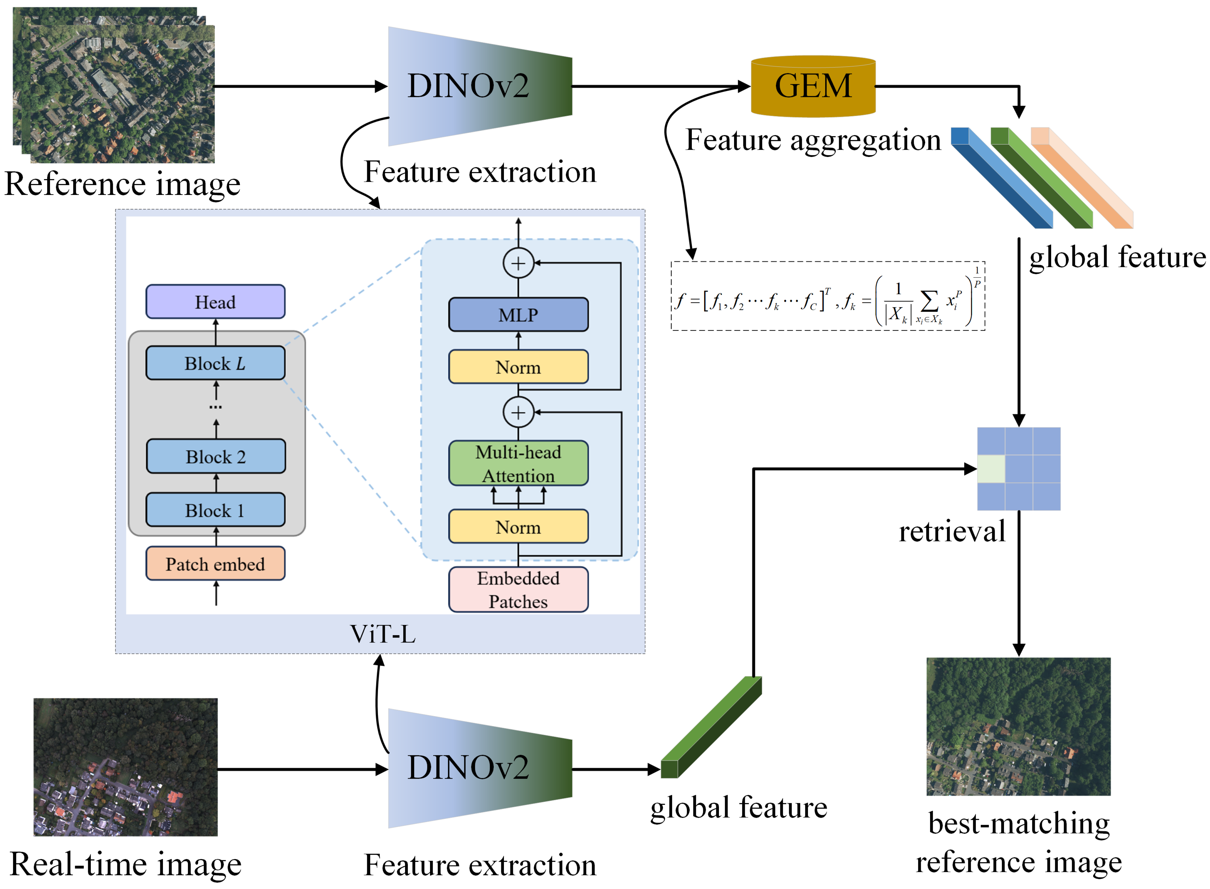
To address these issues, this paper proposes an image retrieval algorithm based on a visual backbone model. The model first extracts generic features using a visual backbone, fully utilizing the spatial information from shallow features and the semantic information from deep features to improve the model’s feature extraction capability. Based on this, a generalized mean pooling method is used to further aggregate the extracted features, enhancing the global feature representation. The overall workflow of the method is shown in Figure 2, consisting mainly of a backbone network and a feature aggregation layer. The backbone network extracts global features from both the real-time image of the UAV and the reference satellite image, while the feature aggregation layer aggregates the extracted features to improve the global expression ability of the feature vectors.

The specific process is divided into two steps.

Offline processing phase: There exists a reference image library. For each image $R_i$, global features $f\left(R_i\right)$ are extracted using the image retrieval model.

Online processing phase: A query image Q (with an original resolution of $1920\times 1080$) is used as a single complete frame and directly fed into the model. Prior to entering the network, the image is uniformly resized to match the input resolution required by the backbone, after which its global feature representation $f\left(Q\right)$ is extracted. The similarity between $f\left(Q\right)$ and $f\left(R_i\right)$ is then computed as $d(Q,R_i)=\parallel f\left(Q\right)-f\left(R_i\right)\parallel .$ The image $R_i$ with the minimum similarity is the retrieval result for the query image Q.

This paper adopts the DINOv2 model as the visual backbone. DINOv2 is based on a Vision Transformer (ViT) architecture and leverages a self-supervised distillation strategy. It has demonstrated strong generalization capabilities in various downstream tasks such as instance retrieval, semantic segmentation, and depth estimation, particularly excelling in zero-shot scenarios. Since training large-scale visual models is extremely costly, this work does not perform additional training on DINOv2 but directly employs its publicly available pre-trained weights. The focus of our study lies in selecting appropriate layers and components from the pre-trained model for feature extraction, and further enhancing retrieval performance through the integration of unsupervised feature aggregation methods. Details regarding the choice of DINOv2, network layers, and feature selection are provided in Section 4.2.1 “Backbone Network Architecture Design”. Furthermore, this work employs unsupervised feature aggregation methods, which construct global image representations by aggregating local features without requiring manual annotations. In Section 4.2.2 “Feature Aggregation Experimental Design”, we compare four aggregation methods—GAP, GMP, GeM, and VLAD—and identify the most effective one for our task.

3.2. Image Registration Algorithm Based on Cycle-Consistency Matching

The performance of image registration directly impacts the accuracy of subsequent visual localization. Most existing image registration algorithms are designed for images captured from ground-based platforms. However, in UAV-based visual localization tasks, it is necessary to match real-time UAV-captured images with satellite reference images. The differences between the two image sources are mainly reflected in the following two aspects.

First, scale discrepancy: Due to the significant altitude difference between satellites and UAVs during image acquisition, the captured images exhibit notable scale variations. This imposes a higher demand on the scale-invariance capability of the image registration algorithm. Second, viewpoint discrepancy: Satellite images are typically captured from a near-vertical (approximately 90°) viewpoint, whereas UAV images are captured from oblique angles, adjustable according to specific mission requirements. This necessitates improved viewpoint consistency in the registration algorithm.

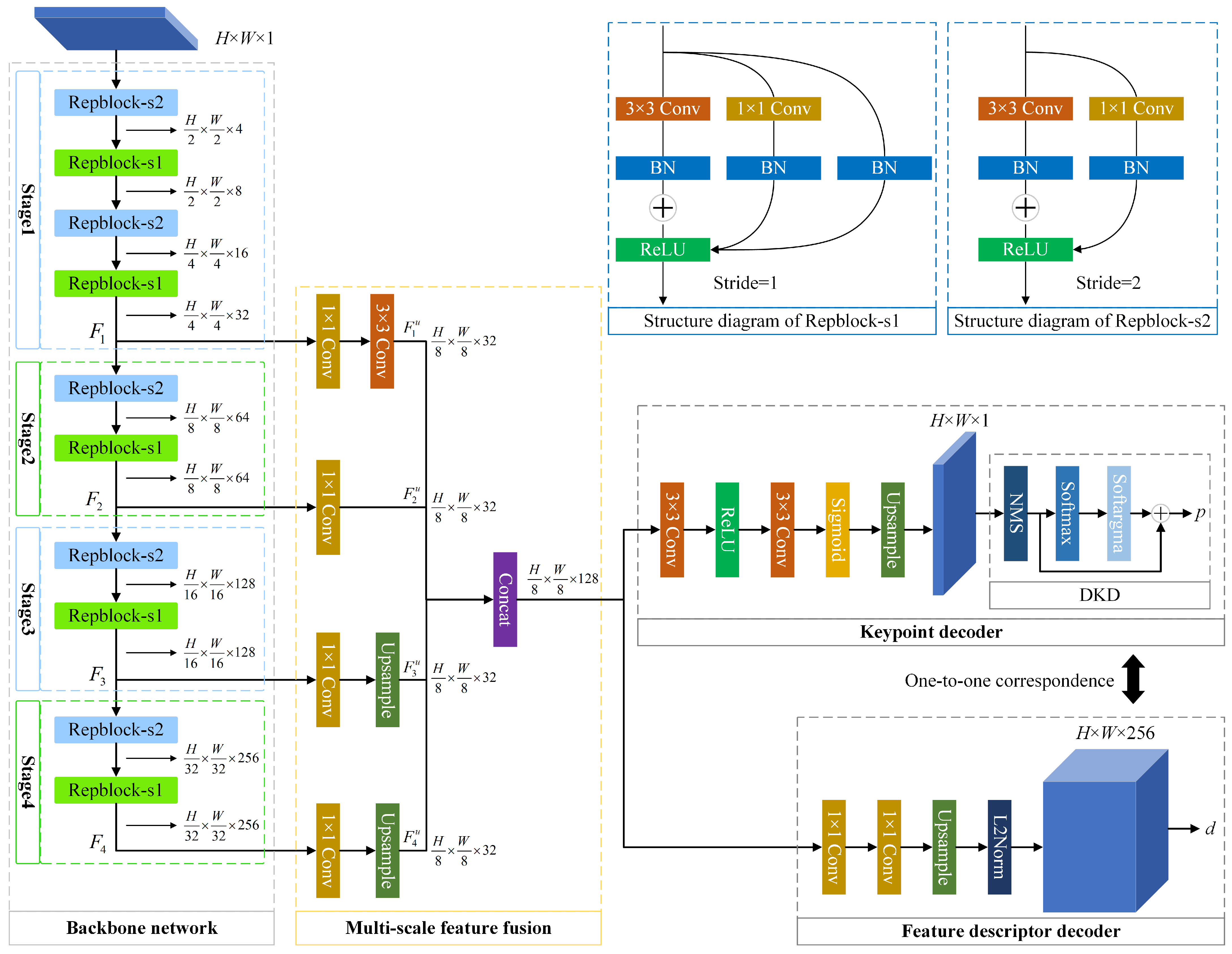
To address these challenges, we propose an image registration algorithm based on cycle-consistency matching. First, we introduce a loss function based on cycle-consistency matching and reprojection error, which optimizes the training process by encouraging the model to learn geometrically and structurally consistent features, thereby improving accuracy. On this basis, we design a multi-scale feature fusion module to enhance the model’s capability to extract features at different scales. Additionally, a structural re-parameterization method is integrated into the image registration algorithm: multiple branches are used during training, while a single branch is employed during inference. This approach improves inference speed while maintaining accuracy. The overall architecture of SuperPoint is modified, with most network parameters shared between the two tasks, enabling reduced overfitting through shared feature representations. In the shared encoder for feature extraction, structural re-parameterization is used to accelerate inference. A feature fusion module is employed to integrate features from multiple scales, improving the model’s ability to extract multi-scale information.

In the keypoint decoder, a differentiable keypoint detection module [46] is incorporated, which allows sub-pixel keypoint locations to be directly optimized via backpropagation. For the loss function, we design a training objective based on cycle-consistency matching and reprojection error to further optimize the model training. The overall architecture is illustrated in Figure 3.

3.2.1. Backbone Network

The encoder of SuperPoint adopts a VGG-style [47] architecture, consisting of multiple stacked 3 × 3 convolutional layers. The 3 × 3 convolutions are well supported and highly optimized on both CPUs and GPUs [48], and their theoretical computational density is approximately four times that of other convolution operations [49]. With the emergence of multi-branch architectures such as Inception and ResNet, the accuracy of deep models has been further improved. However, these multi-branch structures inevitably introduce additional computational complexity. To leverage the benefits of multi-branch architectures while retaining the simplicity and efficiency of the VGG network, this work incorporates a structural re-parameterization approach [50], which decouples the training architecture from the inference architecture. Specifically, multiple branches are employed during training to enhance representational capacity, while a single-branch equivalent is used during inference to maintain accuracy with significantly reduced computational overhead.

In the RepVGG framework, two modules are used during training: a stride-1 module and a stride-2 module for downsampling, referred to as Repblock-s1 and Repblock-s2, respectively, as illustrated in Figure 3. After training, a simple algebraic transformation is applied. In this process, the identity mapping branch can be regarded as an equivalent $1\times 1$ convolution, which can further be reformulated as a degenerated $3\times 3$ convolution. This enables the learned parameters to be consolidated into a single $3\times 3$ convolutional layer for inference. The encoder is organized into four stages comprising a total of ten Repblocks, with ReLU serving as the activation function. The output feature maps after each stage are denoted as ${\mathit{F}}_1$, ${\mathit{F}}_2$, ${\mathit{F}}_3$, and ${\mathit{F}}_4$, with dimensions of ${\displaystyle \frac{H}{4}}\times {\displaystyle \frac{W}{4}}\times 32,{\displaystyle \frac{H}{8}}\times {\displaystyle \frac{W}{8}}\times 64,{\displaystyle \frac{H}{16}}\times {\displaystyle \frac{W}{16}}\times 128,{\displaystyle \frac{H}{32}}\times {\displaystyle \frac{W}{32}}\times 256,$ respectively.

3.2.2. Multi-Scale Feature Fusion

SuperPoint utilizes single-scale features for feature extraction and does not incorporate multi-scale representations, which limits its scale invariance. To address this limitation, this work introduces a feature pyramid structure to enable multi-scale feature fusion, thereby enhancing the model’s robustness to scale variations. In the field of deep learning, integrating multi-scale features through feature pyramids has proven effective for improving network accuracy as demonstrated by models such as FPN [51]. Recent image matching approaches [52,53] have also leveraged hierarchical features to enhance feature representation capabilities. The feature fusion strategy adopted in this work is similar to that in [52], which has shown strong performance in matching tasks.

This module fuses multi-scale features $F_1$, $F_2$, $F_3$, and $F_4$. Each feature map is first processed by a $1\times 1$ convolution layer to adjust its channel dimension. Subsequently, all feature maps are upsampled to a unified spatial resolution of ${\displaystyle \frac{H}{8}}\times {\displaystyle \frac{W}{8}}$. The processed feature maps are denoted as $F_1^u$, $F_2^u$, $F_3^u$, and $F_4^u$.

Finally, by concatenating these rescaled features, both the spatial localization information from shallow layers and the semantic context from deeper layers are fully utilized. The resulting fused feature map has a dimension of ${\displaystyle \frac{H}{8}}\times {\displaystyle \frac{W}{8}}\times 128$, and is computed as

$$F=concat\left(F_1^u,F_2^u,F_3^u,F_4^u\right)$$

(1)

3.2.3. Keypoint Decoder

The input to the keypoint decoder is a feature map of size ${\displaystyle \frac{H}{8}}\times {\displaystyle \frac{W}{8}}\times 128$, and the output is a feature map of size $H\times W\times 1$. This component consists of two convolutional layers, with the last layer using a sigmoid activation function to constrain the output values within the range $[0,1]$, representing the probability of each pixel being a keypoint. The resulting score map is denoted as $\mathit{R}$.

A commonly used approach for obtaining keypoint locations is to apply Non-Maximum Suppression (NMS) to eliminate duplicate detections [54,55,56]. However, this method suffers from a key limitation: the extracted keypoint positions are decoupled from the probability map output by the network, making it impossible to backpropagate gradients during training. To address this issue, we adopt the differentiable keypoint detection (DKD) module proposed in [46], which enables the network to learn keypoints at sub-pixel accuracy. By integrating keypoint detection with probability prediction into a unified task, the network can directly output both keypoint locations and their corresponding confidence scores.

Concretely, for each $H\times N$ window, NMS is first applied to obtain the maximum value within the window, and subsequent steps are performed as follows:

$$r=\left\{\begin{array}{c}{r}_{max},r=r_{max}\\ 0,others\end{array}\right.$$

(2)

The location with the maximum response within the sliding window over the entire image is identified and denoted as ${[u,v]}_{NMS}^T$. The probability values within the local window are then normalized as follows:

$$r^{\prime }(i,j)=\mathrm{softmax}\left({\displaystyle \frac{r(i,j)-r_{max}}{{\tau }_{det}}}\right)$$

(3)

where ${\tau }_{det}$ denotes the temperature coefficient, which controls the smoothness of the output. The softmax function is applied to normalize $\mathit{x}$:

$$\mathrm{softmax}\left(x\right)={\displaystyle \frac{\exp \left(x\right)}{\sum \exp \left(x\right)}}$$

(4)

Subsequently, a softargmax operation is performed to estimate the expected keypoint location within the local window:

$${[\widehat{i},\widehat{j}]}_{soft}^T=\mathrm{softargmax}\left(r^{\prime }(i,j)\right)=\sum _{0\le i,j<N}{r}^{\prime }(i,j){[i,j]}^T$$

(5)

Finally, the sub-pixel keypoint location in the full-resolution image is computed as

$$p={[u,v]}_{soft}^T={[u,v]}_{NMS}^T+{[\widehat{i},\widehat{j}]}_{soft}^T$$

(6)

3.2.4. Feature Descriptor Decoder

The feature descriptor decoder takes as input a feature map of size ${\displaystyle \frac{H}{8}}\times {\displaystyle \frac{W}{8}}\times 128$ and outputs a feature descriptor map of size $H\times W\times D$, where D is the dimension of the descriptor. This component consists of two $1\times 1$ convolutional layers with 128 and 256 channels, respectively, without any activation functions. Before producing the final output, an ${\ell }_2$ normalization operation is applied. Each position in the output feature map corresponds to a descriptor, which aligns one-to-one with the score map $\mathit{R}$ produced by the keypoint decoder.

3.2.5. Loss Function

During the network training process, a multi-task loss function is designed, which consists of three components: keypoint detection loss, descriptor loss, and reprojection loss.

In SuperPoint, the keypoint detection task is formulated as a multi-class classification problem, where only one keypoint is allowed within each $8\times 8$ cell. As a result, the maximum number of SuperPoint keypoints is limited to ${\displaystyle \frac{H\times W}{64}}$. In this work, we adopt the approach introduced in SiLK [57], which considers each pixel as a potential keypoint candidate and redesigns the loss function accordingly.

Given two images, $\mathit{I}$ and ${\mathit{I}}^{\prime }$, with a total of $H\times W=N$ pixels. Let $d_i,d_j^{\prime }\in {\mathbb{R}}^{128}$ represent the descriptors of images $\mathit{I}$ and ${\mathit{I}}^{\prime }$, respectively. Let $r,r^{\prime }\in [0,1]$ denote the predicted keypoint probability. The similarity between descriptors $d_i$ and $d_j^{\prime }$ is represented by $s_{ij}\in [-1,+1]$.

The variables $c_i$ and $c_j^{\prime }$ denote the correspondence between the i-th point in image $\mathit{I}$ and the j-th point in image ${\mathit{I}}^{\prime }$, with a total of M correspondences ($M\le N$). The corresponding keypoints are denoted as $p,p^{\prime }\in {\mathbb{R}}^{2\times M}$. The binary variable y indicates whether the descriptors are successfully matched. We determine correct matches using the simplest mutual nearest neighbor strategy, which is defined as follows:

$$y_i=1\left[s_{c_i{c^{\prime }}_i}\ge \underset{k}{max}\left\{s_{c_{i}k}\right\}\right]1\left[s_{c_i{c^{\prime }}_i}\ge \underset{k}{max}\left\{s_{k{c^{\prime }}_i}\right\}\right]$$

(7)

Here, 1[·] denotes the indicator function. This condition checks whether the current correspondence is mutually the most similar, meaning that the similarity score is the maximum along both its row and column in the similarity matrix. If so, it is considered a successful match. Otherwise, it is regarded as a mismatch.

To further enhance match quality, we employ cycle-consistent matching (CCM), which enforces the idea that two matched features are the closest to each other in the descriptor space. This constraint helps reduce the number of ambiguous or incorrect matches while increasing the proportion of correct ones. The probability of a match being valid is defined as

$$P_{i\leftrightarrow j}=P_{i\to j}{P}_{i\leftarrow j}$$

(8)

Here, the matching probability from descriptor $d_i$ to $d_j^{\prime }$ is defined as $P_{i\to j}={\displaystyle \frac{e^{s_{ij}/\tau }}{{\sum }_k{e}^{s_{ik}/\tau }}},$ and the matching probability from descriptor $d_j^{\prime }$ to $d_i$ is defined as $P_{i\leftarrow j}={\displaystyle \frac{e^{s_{ij}/\tau }}{{\sum }_k{e}^{s_{kj}/\tau }}}.$

The computation follows a scheme similar to the InfoNCE loss commonly used in self-supervised learning [58]. The temperature coefficient $\tau$ is used to modulate the focus on hard negative samples [59]. The similarity matrix $\mathit{s}$ is computed using the standard cosine similarity function.

$$s_{ij}=\mathrm{cosim}(d_i,d_j^{\prime })={\displaystyle \frac{\langle d_i,{d^{\prime }}_j\rangle }{\sqrt{\langle d_i,d_i\rangle \langle {d^{\prime }}_j,{d^{\prime }}_j\rangle }}}$$

(9)

Here, ⟨·, ·⟩ denotes the dot product. The descriptor loss is computed over all matched descriptor pairs as

$${\mathcal{L}}_{desc}=-{\displaystyle \frac{1}{N}}\sum _{i=1}^{N}log{P}_{c_i\leftrightarrow {c^{\prime }}_i}=-{\displaystyle \frac{1}{N}}\sum _{i=1}^N\left[log{P}_{c_i\to c^{\prime }}+log{P}_{c^{\prime }\leftarrow c_i}\right]$$

(10)

The correspondence between descriptors is indicated by the variable y, allowing the use of a standard cross-entropy loss to supervise keypoint detection:

$${\mathcal{L}}_{key}=\mathrm{BCE}(r,y,c)+\mathrm{BCE}(r^{\prime },y,c^{\prime })$$

(11)

where

$$\mathrm{BCE}(r,y,c)=-{\displaystyle \frac{1}{N}}\sum _{i=1}^N\left[y_{i}log{r}_i+(1-y_i)log(1-r_i)\right]$$

(12)

In addition, keypoint positions are further refined by projecting them from image $\mathit{I}$ to image ${\mathit{I}}^{\prime }$ using a homography matrix $\mathbf{H}$ as

$${[p_{I\to I^{\prime }}^T,1]}^T=H_{I\to I^{\prime }}{[p^T,1]}^T$$

(13)

For each transformed keypoint $p_{I\to I^{\prime }}$, we determine whether it matches its corresponding ${\mathit{p}}^{\prime }$ based on a threshold thresh defined in the ground truth. The reprojection error is computed as

$$dis{t}_{I\to I^{\prime }}={∥p_{I\to I^{\prime }}-p^{\prime }∥}_2$$

(14)

Similarly, ${\mathbf{p}}^{\prime }$ can be projected back to image $\mathit{I}$, yielding the point ${\mathbf{p}}_{\mathit{I}\leftarrow {\mathit{I}}^{\prime }}$. The final reprojection loss is defined as

$${\mathcal{L}}_{rep}={\displaystyle \frac{1}{2}}(dis{t}_{I\to I^{\prime }}+dis{t}_{I\leftarrow I^{\prime }})$$

(15)

The total loss is then defined as the weighted sum of the three components:

$$\mathcal{L}={\lambda }_{desc}{\mathcal{L}}_{desc}+{\lambda }_{key}{\mathcal{L}}_{key}+{\lambda }_{rep}{\mathcal{L}}_{rep}$$

(16)

where ${\lambda }_{\mathit{desc}}$, ${\lambda }_{\mathit{key}}$, and ${\lambda }_{\mathit{rep}}$ are weighting factors that balance the contributions of the descriptor loss, keypoint detection loss, and reprojection loss, respectively.

3.3. System Design and Implementation

The entire software system is developed based on the Robot Operating System (ROS). Communication between nodes is achieved via custom-defined message types. The overall system architecture is illustrated in Figure 4. Leveraging the ROS sensor data management framework, the system can acquire sensor data in real time and distribute it to relevant algorithmic modules through inter-node communication. This design allows each component in the system to focus on its specific function, effectively decoupling hardware from algorithmic logic.

The localization algorithm module serves as the core component of the entire system and is primarily composed of five submodules: the Image Preprocessing Node, Map Update Node, Localization Node, Image Registration Node, and Pose Estimation Node. The main functionalities of each node are described as follows.

The Image Preprocessing Node receives real-time UAV imagery and IMU data as inputs, and outputs the preprocessed images. In this module, a real-time image correction strategy based on IMU prior information is proposed.

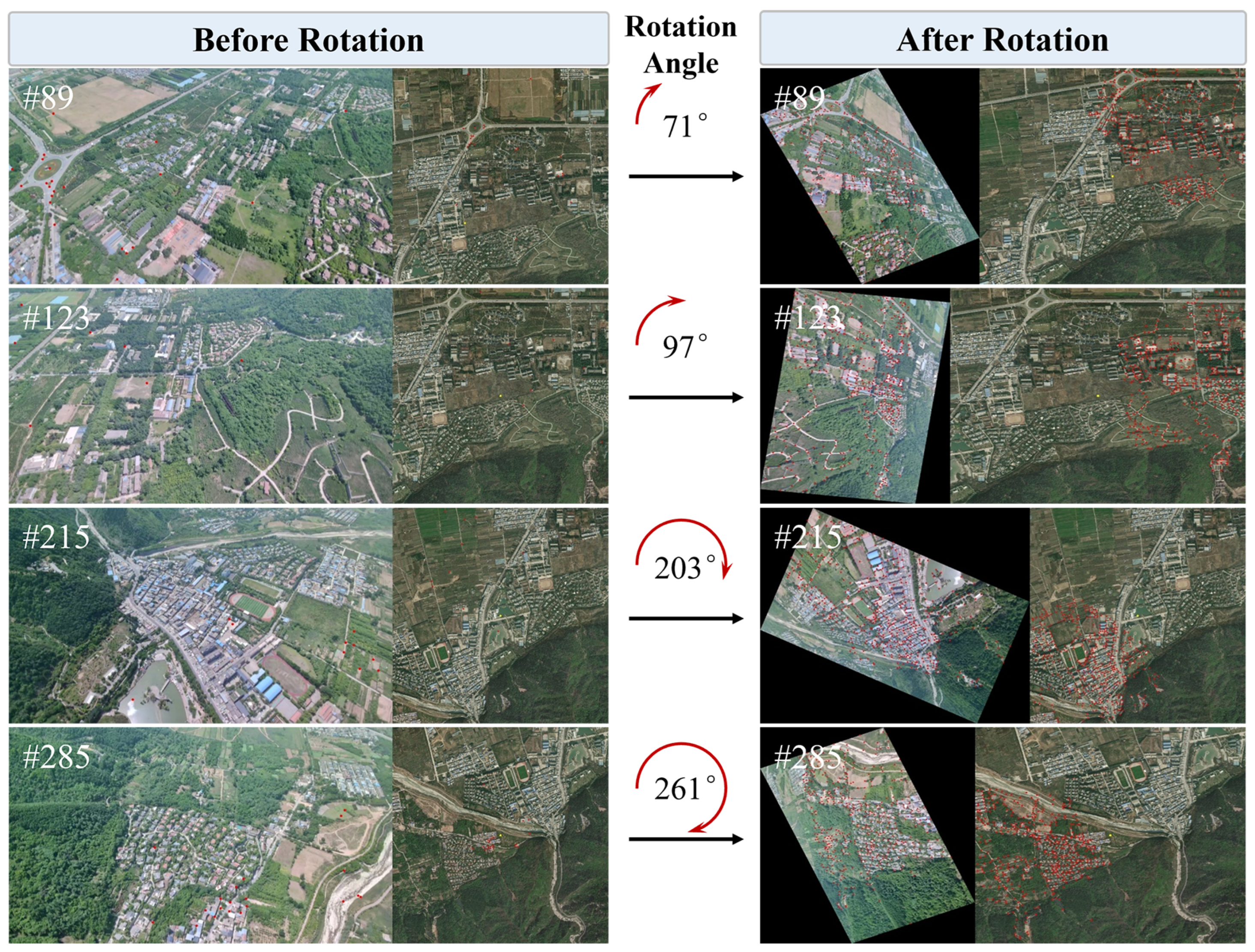
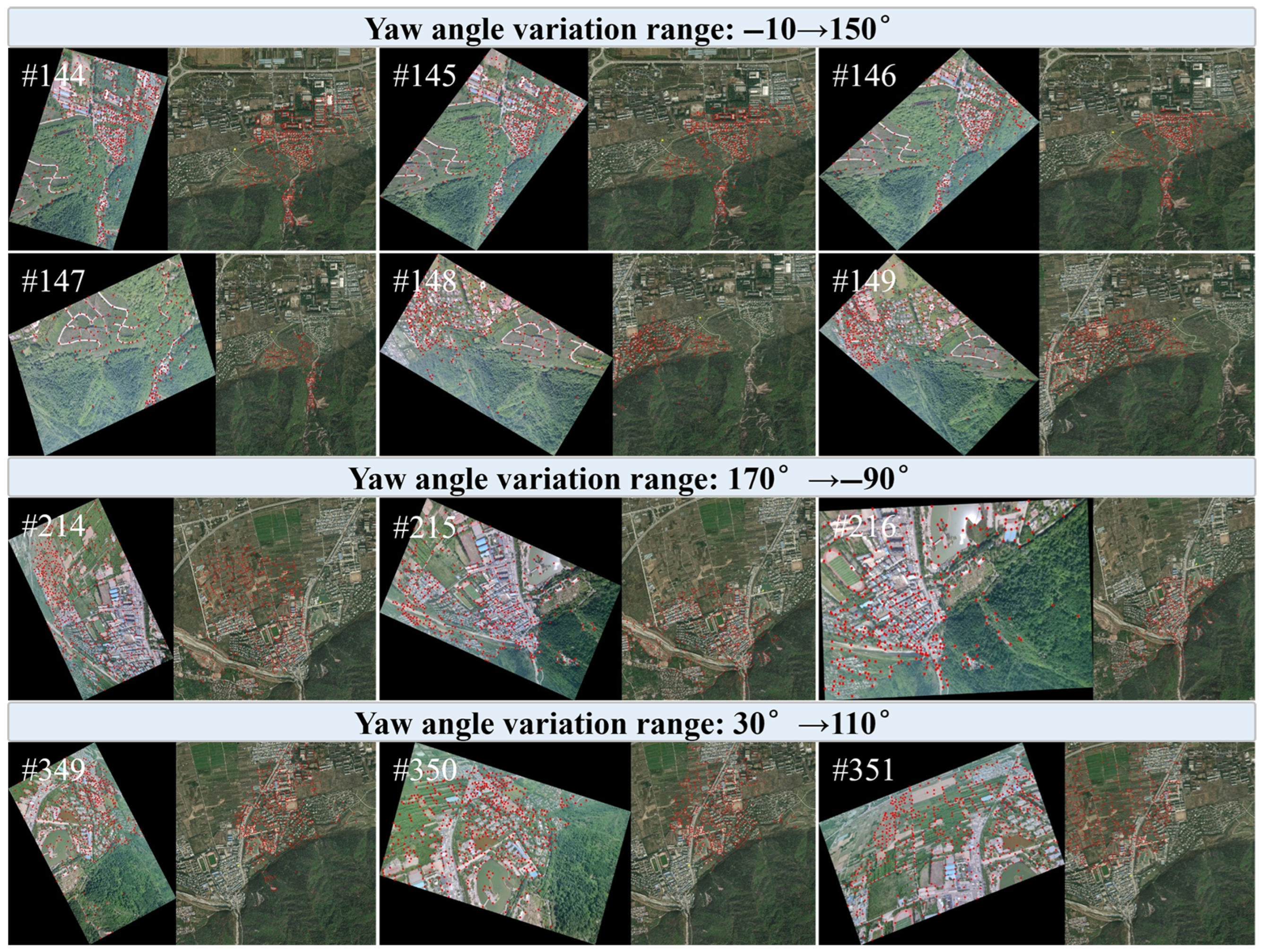
During preprocessing, the image data and IMU data are first temporally synchronized. This is achieved at the software level using functions such as TimeSynchronizer provided by the ROS framework. Additionally, image distortion correction is performed. On top of this, a real-time image correction strategy utilizing IMU priors is applied to align the input image with the reference map. Due to variations in the yaw angle of the UAV during flight, there often exists a rotational discrepancy between the real-time image and the reference image. During UAV flights, dynamic variations in the yaw angle have a significant impact on image registration accuracy. Although the proposed registration algorithm exhibits a certain degree of robustness to rotation, experimental results indicate that this robustness is limited. As shown in Figure 5, when the rotation angle varies within the range of $\pm 30°$, the registration success rate remains relatively high. However, once the angular difference exceeds $\pm 30°$, the number of matched points decreases rapidly, and the error increases substantially. In particular, under large yaw changes of the UAV (e.g., angular differences of $90$ or $180$), effective registration between real-time and reference images becomes nearly impossible (see Figure 5), ultimately leading to localization failure. Considering that low-altitude UAVs often experience unpredictable yaw variations due to mission requirements, relying solely on image registration is insufficient to ensure system robustness.

To address this, we propose a correction approach that computes the rotation matrix ${\mathbf{R}}_C^S$ from the IMU data of the UAV to transform the camera coordinate system into that of the reference map. This matrix is decomposed to obtain the yaw angle ${\theta }_z$, which is then used to adjust the real-time image, minimizing the rotational mismatch between it and the reference.

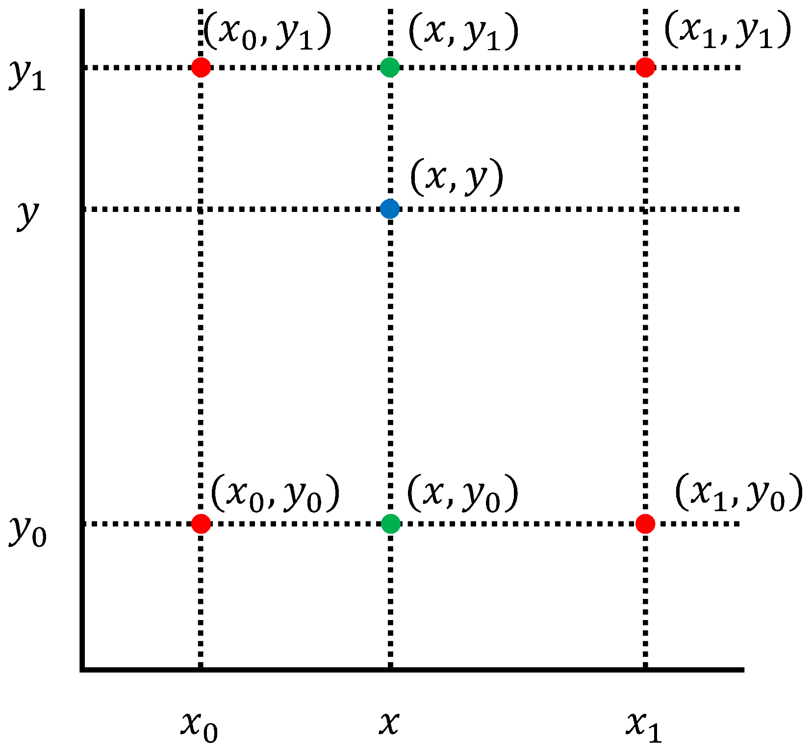
However, during the image rotation process, since image pixels are stored as integers, rotating the image may lead to pixel coordinates with non-integer values, resulting in distortion. To mitigate this issue and preserve image quality, bilinear interpolation [60] is employed to refine the rotated image. As illustrated in Figure 6, bilinear interpolation first performs interpolation along the x-axis, followed by interpolation along the y-axis, ultimately producing a smoothed and accurate estimate of pixel values at non-integer coordinates.

When an image is rotated, part of its content may be cropped if the rotated image exceeds the original image boundaries, leading to information loss. To address this issue, the display bounding box must be recalculated and adjusted during the rotation process to ensure that the rotated image can be fully preserved. As shown in Figure 7, the dashed yellow box denotes the region containing the valid information to be retained, while the red bounding box represents the actual accessible image boundary. After the UAV rotates, if the bounding box size is not adjusted, part of the information within the dashed yellow box will be cropped (middle image). By enlarging the bounding box, all information within the dashed yellow box can be completely preserved (right image). This process enables lossless rotation, ensuring that all image information is retained and reducing matching errors in subsequent registration caused by viewpoint inconsistencies.

The Localization Node is built upon the image retrieval algorithm based on a vision foundation model proposed in this work. Leveraging this algorithm, the system searches for reference sub-images within the reference map database. The input to this node is the real-time image of the UAV, and the output is the retrieved satellite reference sub-image along with its corresponding tile index. The Image Registration Node adopts a novel cycle-consistent matching-based image registration algorithm developed in this paper. This algorithm aligns the real-time image with the retrieved reference sub-image. The inputs are the output from the Map Update Node at time $t-1$ and the output from the Image Preprocessing Node at time t. The outputs are the matched feature point pairs and the estimated homography transformation matrix.

In the Map Update Node, we propose a sliding window-based reference map update strategy. Absolute visual localization requires matching UAV-captured real-time images with pre-stored satellite reference images to achieve precise localization. However, directly matching real-time UAV imagery with the full reference map poses two major challenges:

(1)

The satellite reference map typically covers a vast area, leading to excessive memory consumption. Loading the entire map into memory would impose a heavy burden on system resources.

(2)

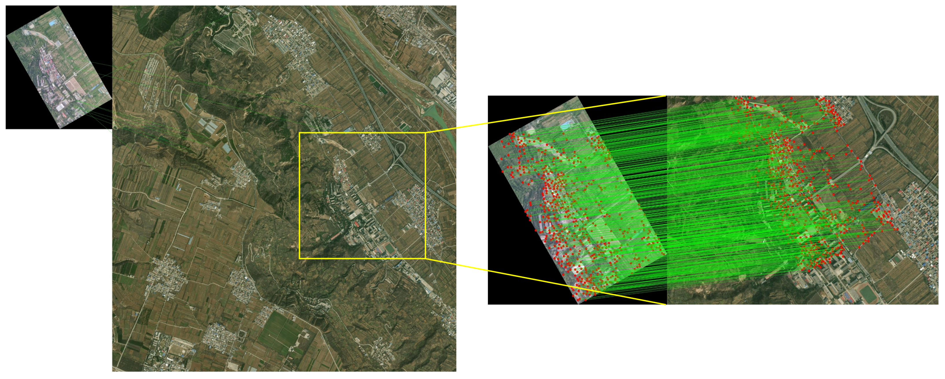
The real-time image of the UAV occupies only a small portion of the satellite reference image, resulting in a considerable scale difference between the two. Direct image registration under such conditions often results in failure as illustrated in Figure 8.

Therefore, the global absolute localization problem can be transformed into a constrained local localization problem under the guidance of prior information—specifically, how to determine the appropriate reference sub-image using prior knowledge and perform accurate UAV localization within that subregion.

Given that UAV flight is continuous in both spatial and temporal domains, there is typically a significant overlap between the real-time image captured at the current moment and that from the previous timestamp. Traditional visual localization methods often assume a nadir-view camera setup, where each pixel in the image is directly associated with a specific ground location. Under this assumption, the reference sub-image for the current frame can be roughly inferred from the last known position of the UAV. However, in this work, we take into full account the impact of the camera pitch angle on localization accuracy in order to enhance system robustness. This consideration means that reference map updates cannot rely solely on the previous localization result. Instead, the system must precisely determine the satellite reference sub-image based on the actual field of view (FOV) presented in the real-time image of the UAV.

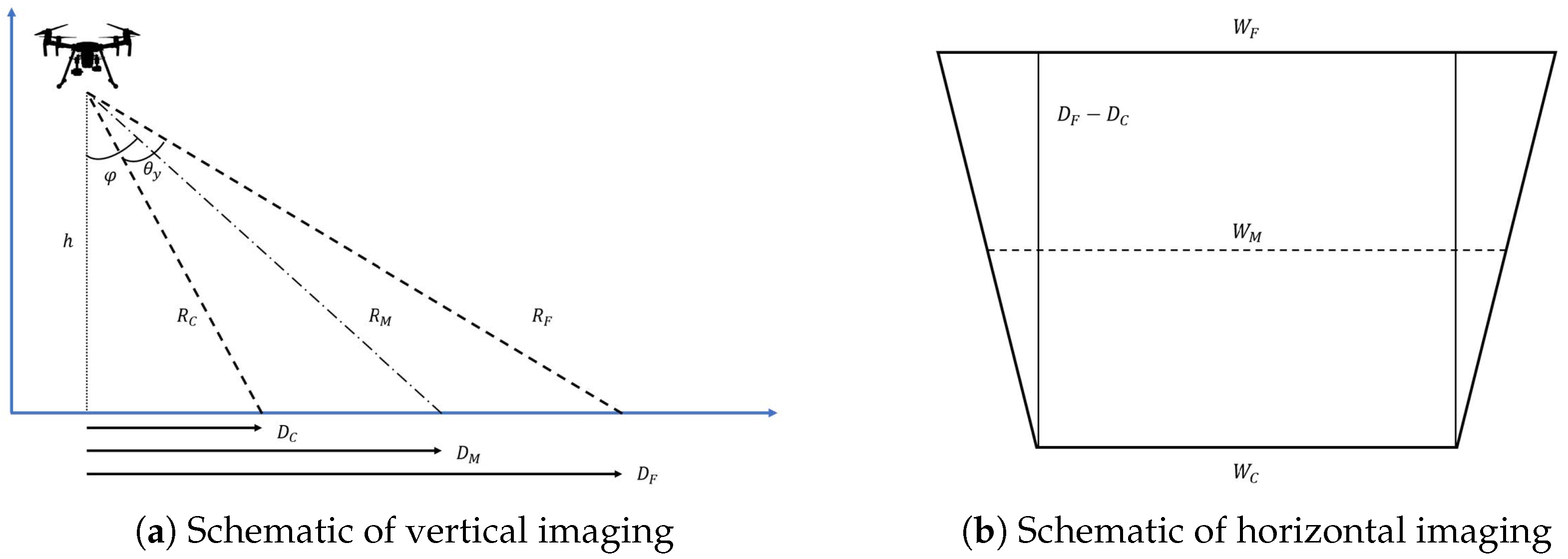
When the camera’s optical axis is not perpendicular to the ground, the imaging range in both vertical and horizontal directions can be calculated according to the camera’s pitch angle ${\theta }_{\mathit{pitch}}$ [61]. As shown in Figure 9, $\phi =90°-{\theta }_{\mathit{pitch}}$, and ${\theta }_x$ and ${\theta }_y$ denote the horizontal and vertical field of view (FOV) angles of the camera in the x and y directions, respectively. The vertical (ground-normal) imaging extent can then be computed using the following expression:

$$\left\{\begin{array}{c}{D}_C=htan\left(\phi -{\displaystyle \frac{{\theta }_y}{2}}\right)\\ D_F=htan\left(\phi +{\displaystyle \frac{{\theta }_y}{2}}\right)\\ D_F-D_C=h\left(tan\left(\phi +{\displaystyle \frac{{\theta }_y}{2}}\right)-tan\left(\phi -{\displaystyle \frac{{\theta }_y}{2}}\right)\right)\end{array}\right.$$

(17)

The projected range in the x-direction (i.e., the horizontal direction in the camera’s field of view) varies with the distance in the y-direction. Therefore, the values of $W_C$, $W_M$, and $W_F$ are derived as follows:

$$\left\{\begin{array}{l}{W}_C=2{\left(D_C^2+h^2\right)}^{1/2}tan\left({\displaystyle \frac{{\theta }_x}{2}}\right)\\ W_M=2{\left({\left({\displaystyle \frac{D_C+D_F}{2}}\right)}^2+h^2\right)}^{1/2}tan\left({\displaystyle \frac{{\theta }_x}{2}}\right)\\ W_F=2{\left({D_F}^2+h^2\right)}^{1/2}tan\left({\displaystyle \frac{{\theta }_x}{2}}\right)\end{array}\right.$$

(18)

When $\phi +{\displaystyle \frac{{\theta }_y}{2}}>90°$, the top of the field of view will be above the horizon. For fields of view above the horizon, the above calculations will no longer be valid.

Based on the previous analysis, the maximum distance at which the camera’s field of view projects onto the ground can be determined. By considering the map’s spatial resolution, the theoretical maximum pixel area $w_{map}$ corresponding to the current frame can then be calculated:

$$w_{map}=\lambda {\displaystyle \frac{W_F}{gs{d}_{map}}}$$

(19)

Here, ${\mathit{gsd}}_{\mathit{map}}$ denotes the spatial resolution of the map, $W_F$ is defined in Equation (18), and $\lambda$ is a hyperparameter used to control the size of the updated map. Its purpose is to mitigate drastic changes in the field of view of the UAV over short time intervals, which could otherwise lead to a failure in reference sub-image coverage. In this paper, $\lambda$ is empirically set to 2.

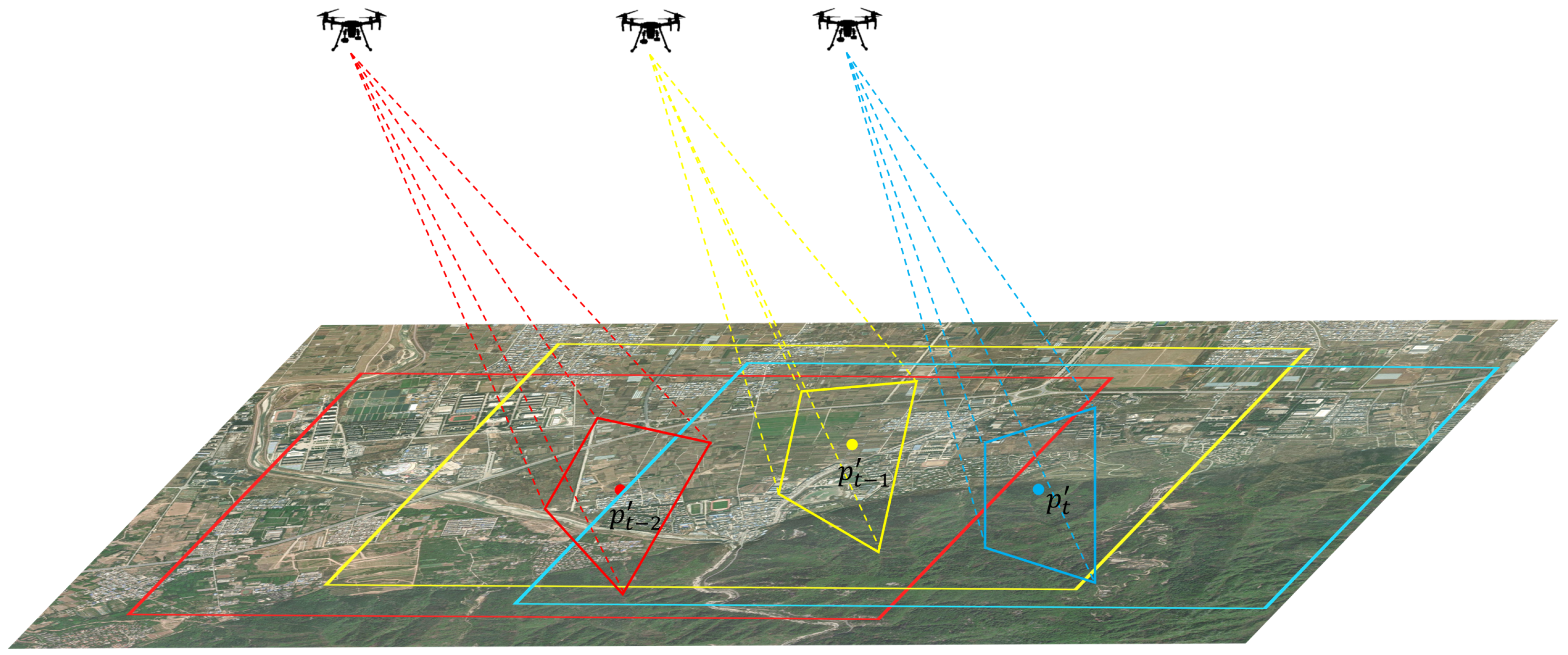
Based on the above calculations, we propose a sliding-window-based reference sub-image update strategy. Given the image center coordinate ${\mathbf{p}}_{t-1}=[u,v]$ and the homography transformation matrix ${\mathbf{H}}_{t-1}$ estimated at time $t-1$, the corresponding coordinate of the image center on the map can be computed as $\left[\begin{array}{c}{\mathbf{p}}_{t-1}^{\prime }\\ 1\end{array}\right]={\mathbf{H}}_{t-1}\left[\begin{array}{c}{\mathbf{p}}_{t-1}\\ 1\end{array}\right].$

Taking ${\mathbf{p}}_{t-1}^{\prime }$ as the center and $w_{\mathit{map}}$ as the side length of a square, we define the region from which the satellite reference sub-image is selected at time t. The detailed selection process is illustrated in Figure 10.

The yellow trapezoid indicates the field of view of the real-time image of the UAV at time $t-1$, projected onto the satellite reference image. The yellow dot represents the coordinate ${\mathbf{p}}_{t-1}^{\prime }$, corresponding to the center of the image of the UAV at time $t-1$ on the reference map. The yellow rectangle denotes the search area for the reference sub-image computed at time $t-1$. Similarly, the red and blue elements follow the same representation logic. In general, the reference sub-image search area computed at time $t-1$ is used as the reference sub-image for time t, forming a progressive relationship across frames. Due to the short time interval, the motion of the UAV from $t-1$ to t is negligible. This ensures that the reference sub-image will fully cover the field of view of the real-time image at time t.

It should be noted that when $H_{t-1}$ contains certain errors, the selection range of the reference sub-image may shift, thereby affecting the accuracy of subsequent matching. To address this issue, the system first degrades into a coarse localization mode. Although the accuracy is reduced, localization continuity can still be maintained. In addition, by incorporating prior information from the IMU and altimeter, further inference and correction can be performed to enhance the robustness of the system. In extreme cases where coarse localization also fails, the error exceeds the designed capability of the system, which constitutes a direction for future research in this work.

In summary, the input to the map update node includes the homography matrix ${\mathbf{H}}_{t-1}$ estimated at time $t-1$ and altimeter data. The output is the reference sub-image at time t.

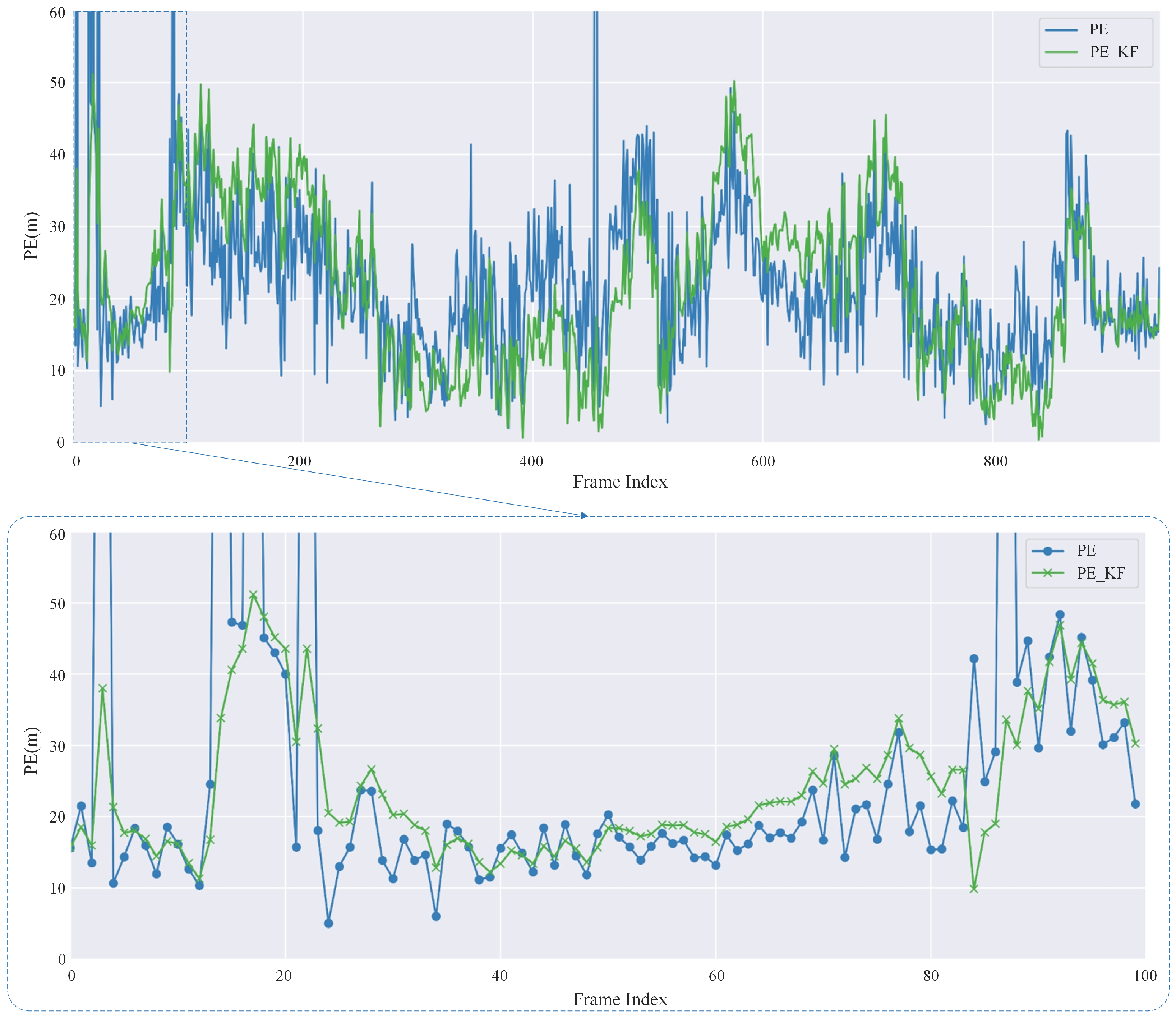
The pose estimation node takes the output from the image registration node as input, computes the pose of the UAV using the Perspective-n-Point (PnP) algorithm, and applies Kalman filtering for refinement. The final output is the estimated pose of the UAV. It should be noted that since the satellite reference map used in this paper is a two-dimensional planar map without elevation information, it is assumed that the height of all points is zero when constructing the 3D spatial points required for the PnP algorithm. Although this simplification neglects terrain variations, it is sufficient for pose estimation in the experimental environment. In addition, the PnP algorithm also relies on camera intrinsic parameters. For the VisLoc dataset used in this paper, we contacted the dataset authors to obtain the camera intrinsics.

4. Experiments

4.1. Experimental Setup

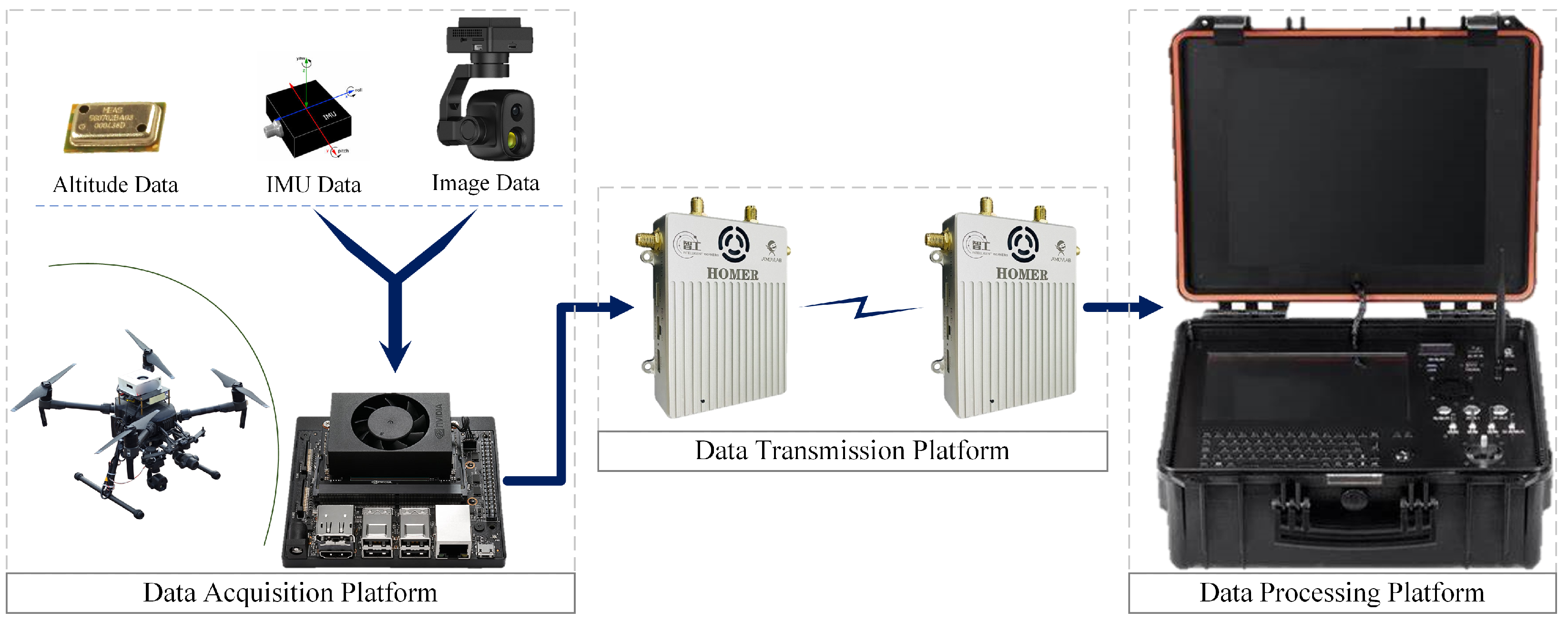
Field tests and validations were conducted in real-world flight environments. The UAV platform used in this study is the DJI M210 (DJI, Shenzhen, China). The onboard camera is a ZT6 dual-sensor gimbal developed by SIYI Technology (Shenzhen, China). The onboard computing unit is an NVIDIA Jetson Xavier NX (NVIDIA, Santa Clara, CA, USA), and digital image transmission is handled by the Homer module from AmovLab (Chengdu, China) (100 Mbps).

The ground control station is equipped with an Intel Core i5-12400 CPU, an RTX 4070 GPU, and 32 GB of RAM. The hardware architecture of the entire system is illustrated in Figure 11.

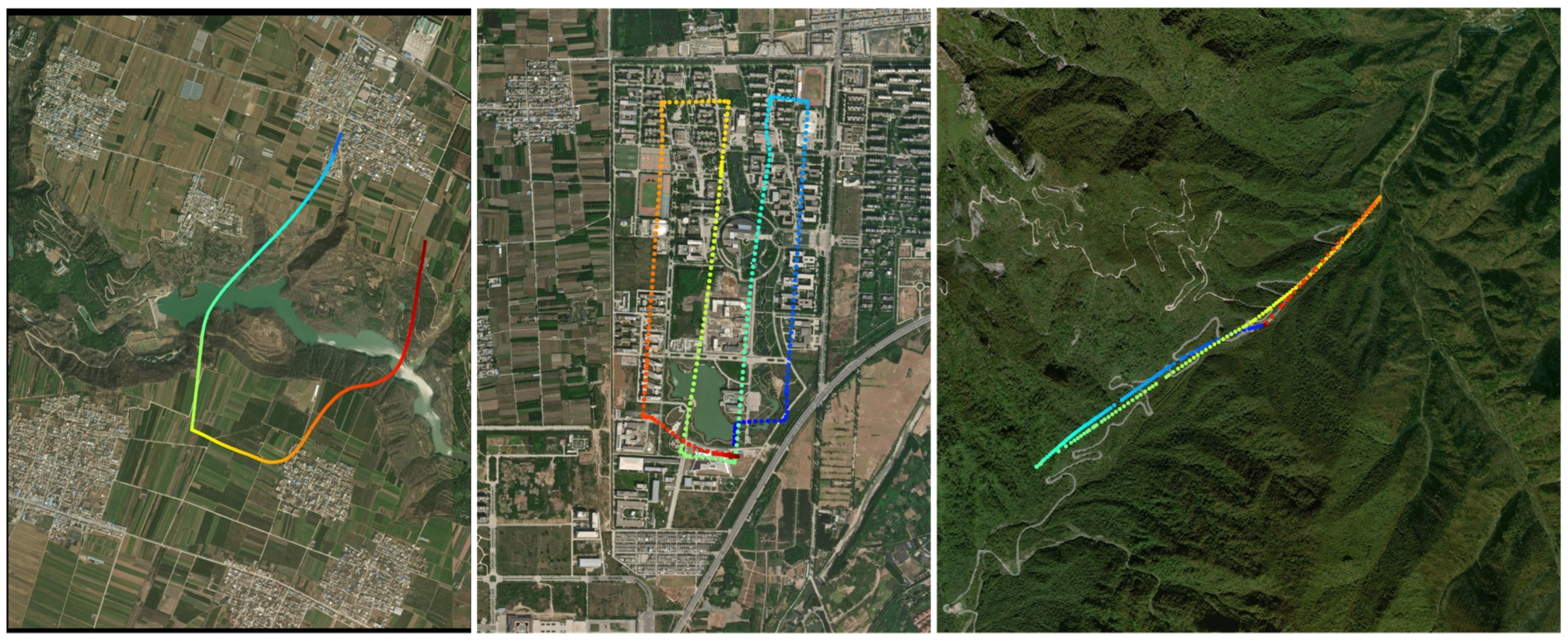
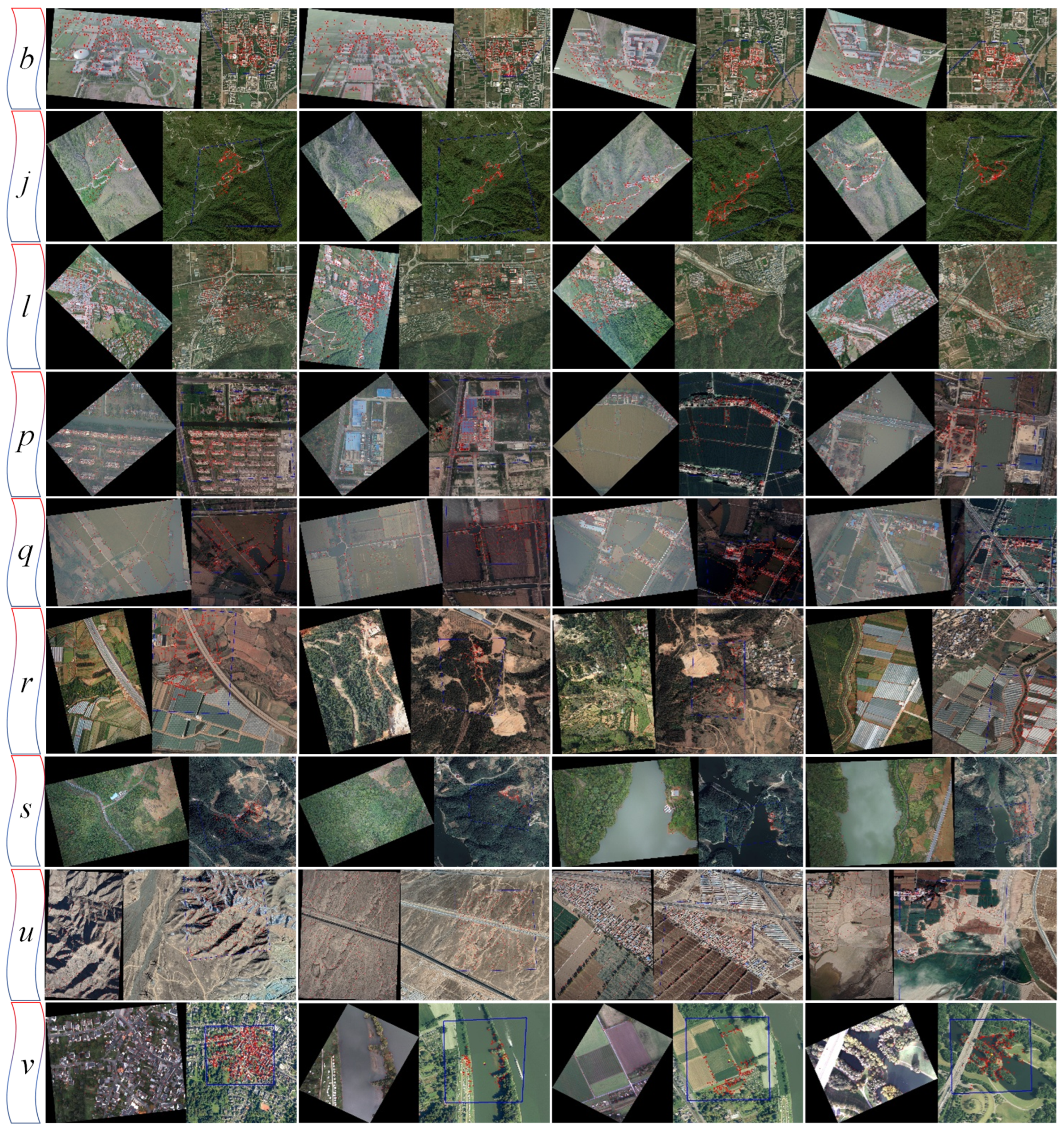
We collected approximately 15,000 aerial images from UAV flights over various regions, each with a resolution of 1920 × 1080 pixels. The collected trajectories are labeled from a to m. An illustration of a subset of the dataset, including the corresponding map and flight paths, is shown in Figure 12, where blue indicates the starting point and red the endpoint. The recorded data includes GNSS information, altitude, timestamp, as well as the pose of the UAV and the gimbal orientation.

The collected images exhibit the following characteristics:

(1)

Diverse terrain coverage, including urban areas, villages, farmland, mountains, rivers, and forests.

(2)

Two main flight altitudes were used: 350 m and 500 m. The gimbal pitch angles included four settings: 30°, 45°, 75°, and 90°. Additionally, the yaw angle of the UAV was varied randomly during flight to evaluate the system’s robustness to rotational changes.

(3)

Data collection was conducted primarily in spring and winter, capturing seasonal variations in appearance.

In addition to our proprietary dataset, we also utilized the publicly available datasets for evaluation, including selected data from VPAir [20] (trajectories v, w, and x) and UAVVisLoc [62] (trajectories n through u). The satellite reference maps used in the experiments were in TIFF format with a spatial resolution of 96 dpi.

We use the Average Absolute Position Error (APE) as the evaluation metric for localization accuracy, measured in meters (m):

$$APE={\displaystyle \frac{{\sum }_{i=1}^n{∥C_i-G_i∥}_2}{n}}$$

(20)

where $C_i$ denotes the UAV position estimated by the localization system, and $G_i$ represents the ground-truth position obtained from GNSS, and n is the total number of frames. The position error (PE) is defined for each single frame as

$$PE={∥C_i-G_i∥}_2$$

(21)

To more comprehensively evaluate the smoothness of the trajectory estimation, the root mean square error (RMSE) metric is further introduced in this paper:

$$RMSE=\sqrt{{\displaystyle \frac{1}{n}}{\sum }_{i=1}^n{∥C_i-G_i∥}_2^2}$$

(22)

Following the definition by He et al. [63], we also define the localization success rate as

$$SucessRate={\displaystyle \frac{{\sum }_{i=1}^{n}1(\epsilon -{∥C_i-C_i∥}_2)}{n}}$$

(23)

Here, $\mathbf{1}(·)$ denotes the indicator function, which outputs 1 when the input is non-negative and 0 otherwise; n represents the number of images; and $\epsilon$ is the decision threshold. In this paper, we follow the AerialVL dataset proposed by He et al. [63], which adopts retrieval distances of 50 m and 100 m as evaluation criteria for aerial absolute visual localization. This choice is mainly due to the fact that aerial scenes typically cover a much larger scale than ground vehicle scenes, thus allowing for a higher tolerance to localization errors. Accordingly, we set $\epsilon =50$. The equation indicates that a localization result is regarded as successful if the average absolute error is less than 50 m, and the success rate is then computed accordingly. Considering the complexity and strong challenges of the dataset used in this work, the system directly regards localization as failed if the first-stage image retrieval is unsuccessful.

4.2. Image Retrieval Algorithm Model Setup

Our experiments are conducted on two publicly available datasets, VPAir and ALTO, mainly to evaluate the impact of different model sizes, depths, feature components, and feature aggregation strategies on retrieval performance. Given the enormous training cost of large-scale models, we do not retrain or fine-tune DINOv2 in this study, but instead directly employ its pre-trained weights.

4.2.1. Backbone Network Architecture Design

This paper adopts the DINOv2 model as the visual backbone. Experiments are conducted on the backbone network, network layers, and feature selection, with the optimal choices made based on the experimental results.

Model Selection

DINOv2 provides four model variants: ViT-S, ViT-B, ViT-L, and ViT-G. The specific parameters of each model are shown in

Table 3. Comparison of parameters for different ViT models.

Model	Layers	Output Dimension	Parameters (M)
ViT-S	12	384	22.06
ViT-B	12	768	86.58
ViT-L	24	1024	304.00
ViT-G	40	1536	1136.00

.

To analyze the impact of models with different parameter scales on the performance of the proposed algorithm in this section, experiments were conducted on the VPAir and ALTO datasets. The models’ performance was evaluated using the Recall@1 and Recall@5 metrics, and the experimental results are presented in Figure 13.

The recall rate generally increases as the model size grows. For the VPAir dataset, although the ViT-G model has nearly three times more parameters than the ViT-L model, its improvement in Recall@1 is only about 10%, indicating that the ViT-G model has a relatively low cost–performance ratio. On the ALTO dataset, the improvement in Recall@1 is not significant, which may be due to excessive overlap between query images and reference images in the ALTO dataset. Compared with ViT-L, the ViT-G model shows only a 6.5% increase in the Recall@5 metric. In contrast, ViT-L demonstrates a noticeable performance improvement over ViT-S and ViT-B on both datasets, indicating that ViT-L achieves a good balance between performance and model size. Therefore, ViT-L is finally selected as the backbone network for the proposed algorithm in this chapter. As shown in the figure, on the VPAir dataset, ViT-L achieves a Recall@1 of approximately 43% and a Recall@5 of around 66%. This performance is comparable to that of existing visual localization methods, such as AnyLoc [24].

Layer Selection

To investigate the impact of features extracted from different layers on the performance of the proposed algorithm, features were extracted from each layer of the ViT-L model for analysis. Tokens were used as the feature representations, and max pooling was adopted as the feature aggregation method. Experiments were conducted on both datasets, and the detailed results are shown in Figure 14.

In the VPAir dataset, Recall@1 steadily increases with the model depth and reaches its peak at layer 23, indicating that deep semantic features contribute positively to retrieval performance. In contrast, the ALTO dataset shows less significant improvement in Recall@1, likely due to its limited scene diversity, which may restrict the effectiveness of semantic information extracted from deeper layers. However, Recall@5 also peaks at layer 23 in the ALTO dataset. Based on these observations, the 23rd layer is selected as the output layer of the ViT-L model in this study.

Feature Selection

Pre-trained ViT models contain rich visual representations. To further explore how different components within a single layer—namely Query, Key, Value, and Token—affect the performance of the algorithm, this study extracts each of these elements from the 23rd layer of ViT-L as feature representations. Max pooling is used as the feature aggregation method, and comparative experiments are conducted on two datasets. The detailed results are shown in

Table 4. Performance comparison of different components as features.

Component	VPAir			ALTO
	R@1 (%)	R@5 (%)	R@10 (%)	R@1 (%)	R@5 (%)	R@10 (%)
Query	31.7	54.5	65.5	12.1	51.2	81.4
Key	34.3	57.0	64.3	11.6	47.9	76.2
Value	48.4	64.5	71.3	6.7	28.6	48.4
Token	47.5	62.5	68.9	5.5	25.7	48.7

.

On the VPAir dataset, the Value and Token components outperform Key and Query across all three metrics, with average improvements of 15% in Recall@1 and 10% in Recall@5. However, the situation is quite the opposite on the ALTO dataset, where Key and Query achieve better performance than Value and Token. On average, Recall@1 and Recall@5 improve by 6% and 20%, respectively, with Recall@1 increasing by as much as 30%. These results suggest that the impact of different components on performance is complex and depends heavily on the specific application scenario. Accordingly, this study selects Value as the output feature for the VPAir dataset and Query for the ALTO dataset.

4.2.2. Unsupervised Feature Aggregation

Based on the results from the previous section, this paper adopts the 23rd layer of ViT-L, with the Value feature selected for the VPAir dataset and the Query feature selected for the ALTO dataset. On this basis, we compare and analyze the impact of four feature aggregation methods—GAP, GMP, GeM, and VLAD—on model performance across both datasets. Detailed results are presented in

Table 5. Performance comparison of different feature aggregation methods.

Pooling Method	Dimension	VPAir			ALTO
		R@1 (%)	R@5 (%)	R@10 (%)	R@1 (%)	R@5 (%)	R@10 (%)
None	1024	43.5	62.5	69.0	4.2	24.2	43.1
GAP	1024	41.6	56.7	63.2	6.4	26.8	46.3
GMP	1024	48.4	64.5	71.3	12.1	51.2	81.4
GeM	1024	50.1	64.0	70.7	14.0	58.1	84.4
VLAD	24,576	53.5	71.9	79.6	14.8	43.9	47.5

.

As shown in Table 5, the use of Global Average Pooling (GAP) not only fails to improve model performance but also leads to a noticeable decline in all evaluation metrics. This degradation may be attributed to the excessive smoothing of feature information during the averaging process, which diminishes feature discriminability. In contrast, the incorporation of GMP, GeM, and VLAD significantly enhances model performance in terms of Recall@1. Among these, VLAD achieves the best overall performance, followed by GeM. This can be explained by the differing capabilities of these methods in modeling feature distributions: VLAD learns local feature distribution patterns through clustering, GeM dynamically adjusts feature aggregation weights via learnable parameters, whereas GMP focuses solely on the strongest local responses, potentially discarding useful information.

Further analysis of the results reveals that VLAD performs notably well on the VPAir dataset but is outperformed by GeM on the ALTO dataset. This discrepancy suggests that VLAD lacks robustness and adaptability across different scenarios. Moreover, VLAD requires manual specification of the number of cluster centers, which increases the complexity of model tuning. Additionally, the high dimensionality of VLAD-generated vectors incurs greater computational and storage costs.

Therefore, GeM is ultimately selected as the feature aggregation method in this study. This choice not only ensures strong model performance but also effectively controls computational resource consumption, offering better practical applicability.

4.2.3. Comparison with Existing Methods

This study focuses on large-scale image retrieval, and the comparative experiments primarily involve widely adopted global representation methods for this task. Specifically, three supervised models are selected: NetVLAD, CosPlace, and MixVPR. In addition, two unsupervised models, DINO and DINOv2, are included for comparison. The backbone network of NetVLAD is VGG-16, while both CosPlace and MixVPR adopt ResNet50. For the unsupervised approaches, DINO employs the ViT-S/8 model and DINOv2 employs the ViT-L model.

As shown in

Table 6. Comparison with state-of-the-art methods.

Model	VPAir			ALTO
	R@1 (%)	R@5 (%)	R@10 (%)	R@1 (%)	R@5 (%)	R@10 (%)
NetVLAD	9.8	19.4	25.5	6.2	23.7	43.6
CosPlace	17.0	32.4	42.1	6.5	28.9	47.4
MixVPR	12.0	21.6	28.2	8.5	40.7	65.0
DINO	35.0	48.4	57.4	3.3	13.4	25.0
DINOv2	43.5	62.5	69.0	4.2	24.2	43.1
Ours	50.1	64.0	70.7	14.0	58.1	84.4

, on the VPAir dataset, the supervised methods (NetVLAD, CosPlace, and MixVPR) exhibit overall inferior performance, which may be attributed to their strong reliance on annotated information and limited adaptability to complex ground scenes. In contrast, the self-supervised models (DINO and DINOv2) demonstrate stronger generalization ability. Building upon this, our method achieves further improvements, outperforming DINOv2 by 6.6%, 1.5%, and 1.7% in R@1, R@5, and R@10, respectively, with the gain in R@1 being particularly significant. On the ALTO dataset, the trend is different: supervised methods perform better under relatively homogeneous scene categories. Nevertheless, our method still surpasses them, not only improving upon DINOv2 but also outperforming the best supervised model MixVPR by 5.5%, 17.4%, and 19.4% in R@1, R@5, and R@10, respectively. It should be noted that the retrieval metric Recall@k used in this section evaluates the performance of image retrieval (i.e., coarse localization), rather than the entire localization system. In later sections, we employ the success rate metric, which jointly considers both the retrieval stage and the subsequent fine localization stage, thereby providing a measure of the overall system accuracy. In summary, our method achieves significant advantages across both datasets, verifying its robustness in complex scenarios as well as its adaptability to diverse scene distributions.

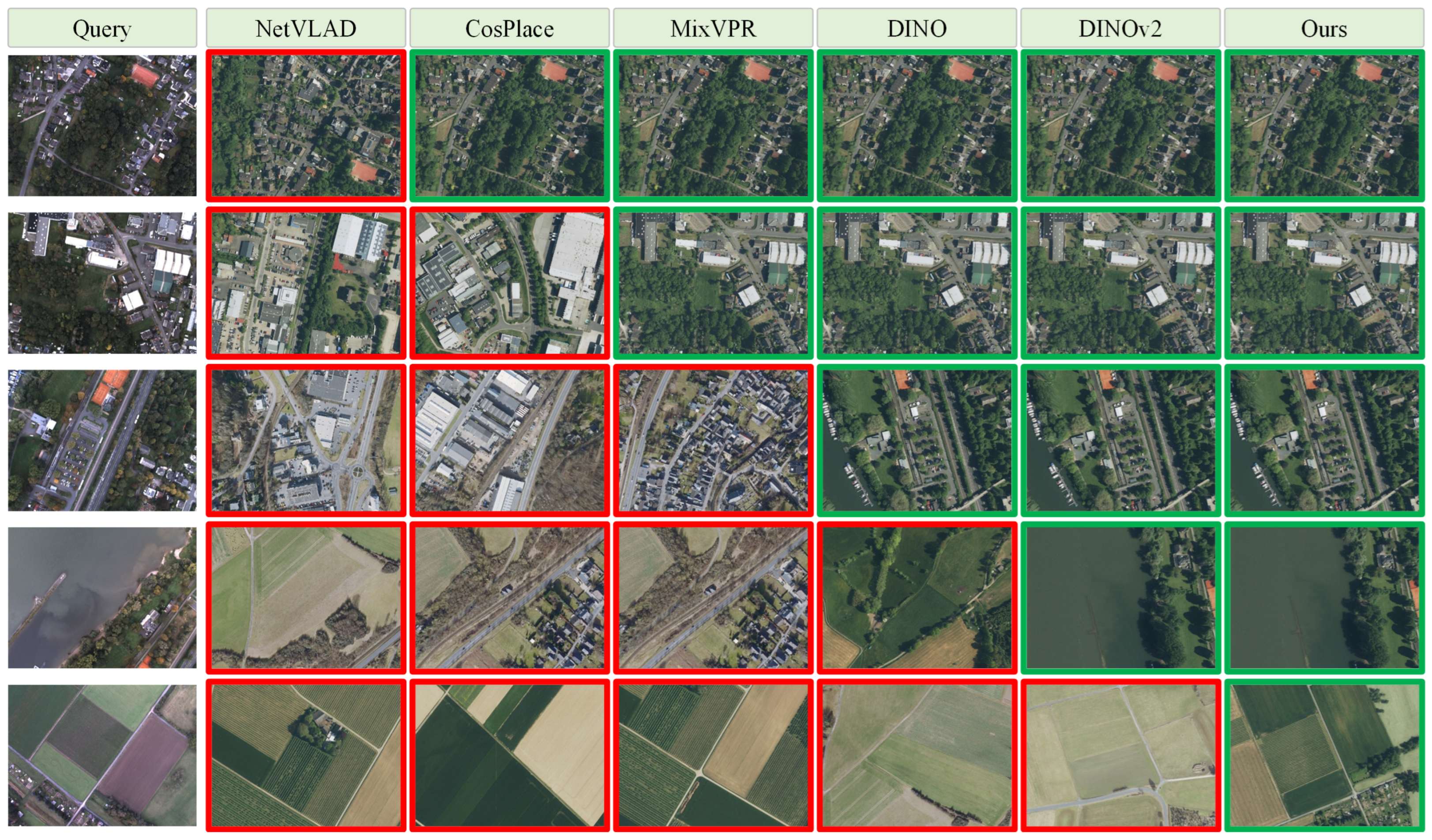
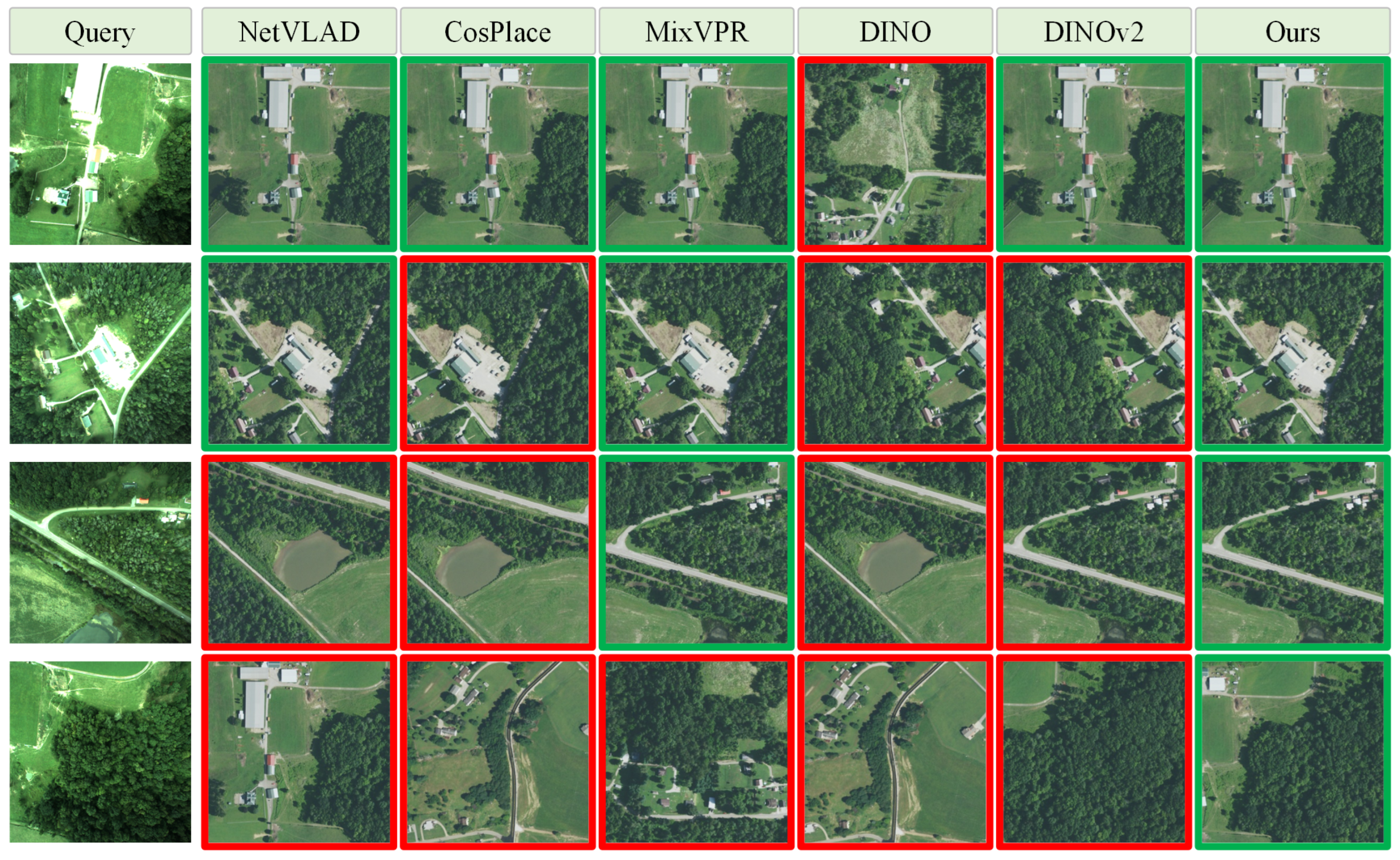
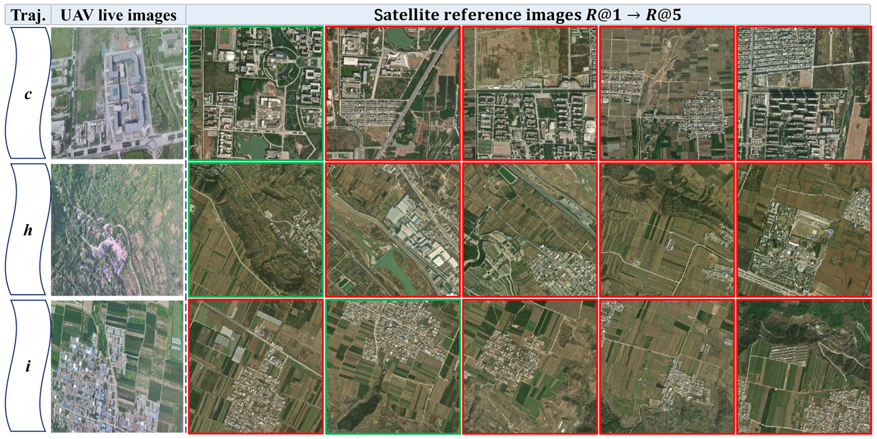
In the visualization of experimental results, correctly retrieved images are highlighted with green bounding boxes, while incorrect results are marked with red bounding boxes. To comprehensively evaluate algorithm performance, we select query images from a variety of representative scenes, including urban areas, rivers, farmlands, and forests, ensuring diversity in the testing process. As illustrated in Figure 15, for query images containing landmark buildings or salient features, all methods achieve relatively high retrieval accuracy. However, in feature-sparse scenes such as rivers and farmlands, the performance of traditional supervised methods drops significantly. This is mainly because they struggle to discriminate between subtle visual differences and rely heavily on the distribution of the training data. In contrast, our method leverages the advantages of pre-trained visual foundation models, enabling it to maintain high performance even in such challenging scenarios.

As shown in Figure 16, the ALTO dataset contains relatively homogeneous scene categories, which leads to suboptimal performance for self-supervised models such as DINO and DINOv2, while supervised methods including NetVLAD, CosPlace, and MixVPR perform comparatively better. Nevertheless, their advantage is strongly tied to specific annotation distributions and thus lacks generalization capability. Our method consistently outperforms all compared models on this dataset. By avoiding reliance on annotations and optimizing both feature extraction and aggregation strategies, it achieves a better balance between generalization and scene adaptability, thereby demonstrating greater practical value.

4.3. Ablation Studies

4.3.1. Impact of Map Resolution on Localization Accuracy

To investigate the impact of map resolution on localization performance, we conducted a controlled experiment in which the UAV flight trajectories were kept constant while only the map resolution was varied. Specifically, we evaluated localization accuracy using maps at three zoom levels: Level 16, Level 17, and Level 18.

As shown in

Table 7. Impact of map resolution on the localization system.

Trajectory	Image GSD (m)	Map Zoom Level	Map Resolution (m)	Map Size (MB)	Success Rate (%)	APE (m)
e	0.62	16	1.980	9.01	88.34	18.90
		17	0.990	33.00	94.90	12.74
		18	0.495	126.00	95.81	12.52
i	0.88	16	1.980	20.02	74.50	15.22
		17	0.990	67.54	79.31	12.41
		18	0.495	245.07	79.31	11.61

, selecting a map zoom level with a spatial resolution close to that of the UAV imagery generally yields better localization performance. Specifically, maps at zoom level 16 exhibit significantly lower localization success rates and accuracy due to the large resolution mismatch with the aerial images. While both zoom levels 17 and 18 achieve comparable localization accuracy and success rates, the map at level 18 requires approximately four times more storage than level 17, leading to higher demands on computational and storage resources. Therefore, all subsequent experiments in this study use zoom level 17 as the default reference map. In practical applications, the choice of map resolution should be made based on the camera’s intrinsic parameters and the flight altitude of the UAV, in order to balance localization accuracy and system resource efficiency.

4.3.2. Impact of Reference Sub-Image Update Strategy on Localization

In large-scale scenarios, the size of the reference map increases proportionally with the coverage area. If the real-time image is directly registered with an excessively large reference map, it not only leads to a significant drop in computational efficiency but may also fail due to insufficient computational resources, making it difficult to meet real-time processing requirements. Moreover, there may exist scale differences of several tens to even hundreds of times between the real-time image and the reference map, which can severely degrade registration accuracy and even result in complete registration failure. To evaluate the effectiveness of the proposed sliding-window-based reference sub-image update strategy, we conducted comparative experiments using two different approaches: one method dynamically adjusts the size of the reference map based on the estimated position of the UAV (our proposed strategy); the other uses a fixed-size reference map throughout the entire localization process. The results are summarized in

Table 8. Impact of reference sub-image update strategy on localization performance.

Trajectory	Reference Update Enabled	Reference Image Size (pixel)	Success Rate (%)	Localization Time (s)	APE (m)
d	✓	1025 × 1025	99.40	0.068	12.21
	×	2816 × 3072	5.36	0.158	24.05
k	✓	1813 × 1813	99.50	0.075	10.47
	×	5632 × 4352	31.82	0.211	17.15
m	✓	4000 × 4000	82.06	0.183	19.96
	×	9774 × 2676	—	—	—
u	✓	4000 × 4000	88.64	0.174	23.71
	×	29,592 × 16,582	—	—	—

.

As shown in Table 8, when the size of the reference map is relatively small (i.e., smaller than 10,000 × 10,000), the probability of successful matching is low without employing the reference sub-map update strategy. Moreover, the matching performance exhibits strong randomness, which compromises the robustness and accuracy of localization. Even in cases where matching succeeds, the larger size of the reference map significantly increases the time required for image registration—typically 2 to 3 times longer than that with the sub-map update strategy. When the reference map size increases to 10,000 × 10,000, the real-time image can no longer be registered with the reference map in the absence of the sub-map update strategy. Under such circumstances, the importance of the reference sub-map update strategy becomes more pronounced. Furthermore, the system achieves a localization frame rate of approximately 15 FPS, demonstrating a certain level of practical applicability. In the overall system, image retrieval is performed only once during initialization on the first frame to determine the initial position, which constitutes a one-time computational cost. Subsequent localization relies on fine registration within the updated reference sub-map, where the size of the local image remains within a reasonable range. This ensures that the fine registration stage can consistently achieve a processing speed of approximately 15 FPS on the ground station equipped with an RTX 4070 GPU (NVIDIA, Santa Clara, CA, USA). The onboard computing unit is an NVIDIA Jetson Xavier NX (NVIDIA, Santa Clara, CA, USA), and digital image transmission is handled by the Homer module from AmovLab (Chengdu, China) (100 Mbps).

It is worth noting that the original resolution of UAV images is $1920\times 1080$, and prior to being fed into the DINOv2 backbone network, they are uniformly resized to $518\times 518$ to ensure efficiency in feature extraction and registration. During 1080 p UAV video transmission, the video data are compressed using the H.264 format with a compression ratio of approximately 300, and the link bandwidth is 100 Mbps. Theoretically, the overall latency of transmission and codec is estimated to be about 30 ms. In practical tests, considering factors such as environment and transmission distance, the latency ranges from 26 to 52 ms, which ensures stable data transmission at a processing rate of around 15 FPS.

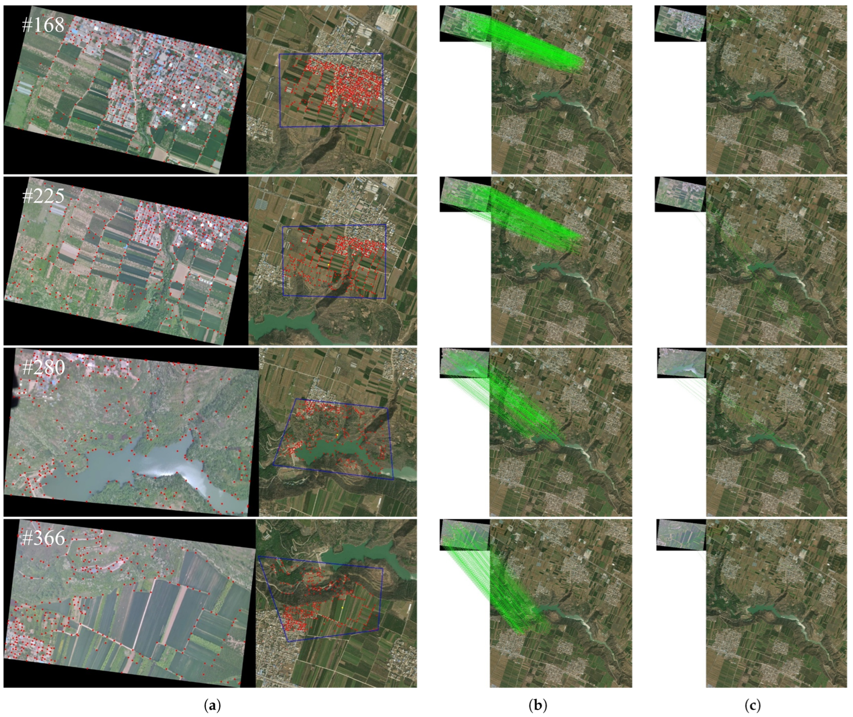
Taking trajectory i as an example, the process of matching with the reference sub-map update strategy is visualized. As shown in Figure 17, the white number in the upper-left corner indicates the frame index of the corresponding real-time image. Figure 17a illustrates the matching process between the real-time image and the dynamically updated reference sub-map, where the right-hand side reference map is updated adaptively. Figure 17b shows the mapping result of Figure 17a projected back onto the original reference map. Figure 17c presents a comparison where the real-time image is directly matched with the original reference map without using the update strategy.

At the initial stage of trajectory i, the UAV remains stationary until it climbs to an altitude of 500 m. Only after reaching the target altitude does it begin its official flight. As shown in Figure 18, during the continuous ascent of the UAV, the satellite reference image is dynamically updated in real time. With the reference sub-image update strategy in place, the display range of the reference image can be adjusted dynamically based on the real-time altitude information of the UAV. This ensures that the reference image consistently covers the live onboard image, thereby guaranteeing the continuous and stable operation of the localization system.

In summary, the proposed reference sub-image update strategy effectively improves both the efficiency and accuracy of localization, while also addressing the challenge of selecting appropriate reference images in large-scale scenes.

4.3.3. Impact of Real-Time Image Rectification Strategy on Localization

To evaluate the effect of the proposed real-time image rectification strategy based on IMU prior information, we conducted comparative experiments. During actual UAV flights, roll and pitch angles are typically adjusted dynamically by the flight control system to maintain stability according to predefined settings. These adjustments have relatively minor effects on the final localization accuracy. Therefore, for simplicity, this study focuses on the impact of yaw angle variations, which are more significant for image alignment. Four flight trajectories were selected for comparative analysis. Two methods were evaluated: one with the proposed image rectification strategy, and the other without it. The experimental results are summarized in

Table 9. Impact of real-time image rectification strategy on localization performance.

Trajectory	Rectification Applied	Yaw Angle Range (°)	Success Rate (%)	APE (m)
b	✓	[−110, −100], [60, 80]	100	10.65
	×		81.02	13.09
l	✓	[−150, −80], [30, 100]	89.16	19.18
	×		31.75	18.09
p	✓	[−40, 120]	99.48	18.57
	×		31.77	17.96
t	✓	[−80, −70], [90, 120]	65.61	19.14
	×		0.24	32.51

.

For trajectory b, significant yaw angle variations only occur during the return segment at the end of the flight. As a result, even without applying the real-time image rectification strategy, the system is still able to localize successfully during the earlier segments with stable yaw angles. In contrast, trajectories l, p, and t experience frequent and large yaw angle variations throughout the flight, leading to a substantial drop in localization success rate when the rectification strategy is not employed. This highlights the effectiveness of the proposed real-time image rectification strategy in improving localization robustness under severe yaw fluctuations.

Taking trajectory l as an example, we visualize and compare the localization results with and without the rectification strategy. As shown in Figure 19, the left image presents the matching results without applying the rectification strategy, while the right image shows the results with it. It is evident that the number of correct matching point pairs significantly increases when the rectification strategy is used, leading to a noticeable improvement in localization success.

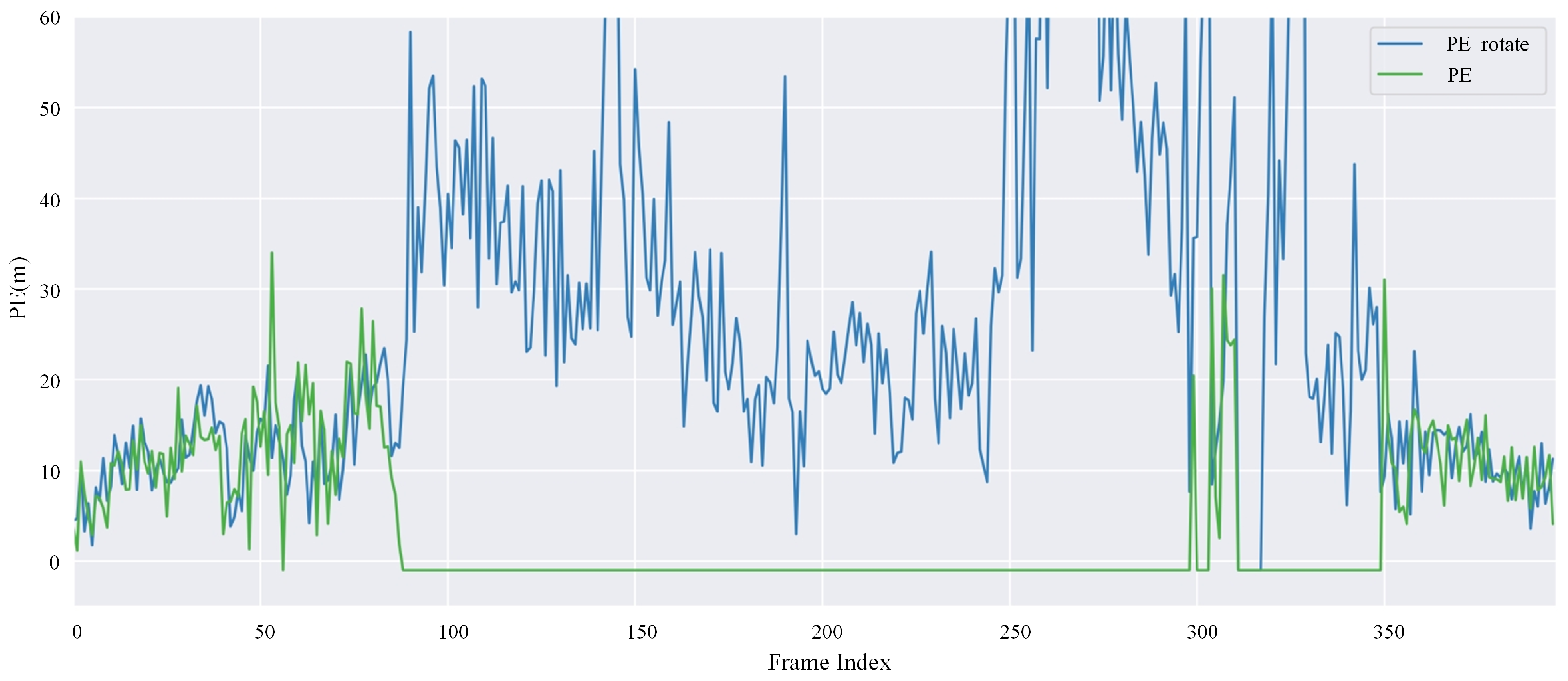
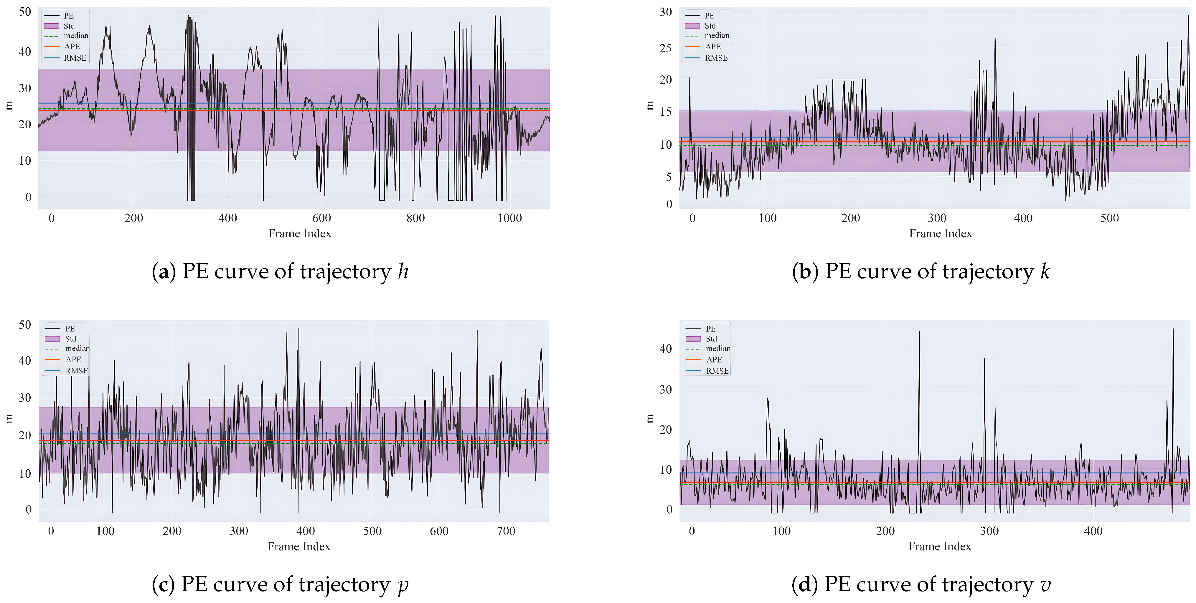
The Absolute Positioning Error (APE) curves for trajectory l are also visualized as shown in Figure 20. The green curve represents the APE without applying the real-time image rectification strategy, while the blue curve shows the APE with the strategy applied. For frames where localization fails, the APE is set to −1. It can be observed that during the period of continuous yaw variation—specifically from frame 89 to around frame 300—the system fails to maintain localization without the rectification strategy. This is due to the system’s inability to adapt to the ongoing changes in yaw angle, resulting in persistent localization failure.

In addition, a segment of trajectory l with continuously varying yaw angles is selected for visualization of the matching results as shown in Figure 21. It can be seen that after incorporating IMU prior information, the system is able to smoothly and adaptively handle the yaw angle changes in real time, thereby significantly enhancing the robustness of the localization system.

4.3.4. Impact of Camera Pitch Angle on Localization Performance

To further investigate how different camera pitch angles affect the localization accuracy of the proposed system, we conducted comparative tests using 7 trajectories across 2 identical scenes. Trajectories a to d belong to one scene, while trajectories f to h belong to another. However, due to various uncontrollable factors in actual UAV operations, it is difficult to ensure that the flight paths are completely identical. As a result, the test results inevitably include some degree of measurement error. Despite this, the experimental outcomes still offer valuable insights into the influence of varying pitch angles on localization performance. As shown in

Table 10. Impact of camera pitch angle on localization performance.

Trajectory	Pitch Angle (°)	Success Rate (%)	APE (m)	Std. Deviation (m)
$\alpha$	30	62.77	31.32	12.92
b	45	79.31	21.65	9.28
c	75	90.69	15.86	7.63
d	90	99.45	12.21	5.95
f	30	27.61	27.71	12.14
g	45	54.28	28.92	9.20
h	90	95.02	23.61	9.27

, the results demonstrate the robustness of the proposed localization system under different pitch angle settings. Specifically, the system is able to consistently accomplish localization tasks regardless of pitch angle variations.

Further analysis of the data reveals a clear trend: when the camera pitch angle is 90°, both the localization success rate and positioning accuracy reach their optimal levels. As the pitch angle decreases, there is a gradual decline in both metrics. Specifically, when the pitch angle is 30°, according to Equation (18), we observe that $\phi +{\displaystyle \frac{{\theta }_y}{2}}>90$°, indicating that the real-time image contains information above the horizon, i.e., the sky region. However, such content is absent in satellite reference images, which primarily depict ground-level scenes. This mismatch leads to missing or redundant information during the image matching process, thereby degrading the accuracy and stability of localization. As a result, both the success rate and localization precision of the system suffer noticeable declines.

In conclusion, for real-world applications, it is essential to ensure that the field of view of the UAV predominantly covers ground-level areas. This maximizes the utility of real-time image content during matching with satellite reference maps, ultimately enhancing the precision and robustness of the localization system.

4.3.5. Impact of Kalman Filtering on Localization Performance

To address the potential influence of noise on localization results, this study employs a Kalman filter algorithm to predict and correct the localization outputs. By mitigating the impact of noise, the filter aims to enhance positioning accuracy. Comparative experiments were conducted with filter parameters set to Q = 0.5 and R = 1. The results are presented in

Table 11. Impact of Kalman filtering on localization performance.

Trajectory	Filter Applied	Success Rate (%)	APE (m)	Std. Deviation (m)
c	✓	99.69	17.86	7.63
	×	98.10	19.91	15.34
p	✓	99.48	18.57	19.14
	×	95.57	23.16	28.51

. Two trajectories were selected for experimental validation. The application of the Kalman filter resulted in a slight improvement in localization success rate and a notable reduction in standard deviation, indicating enhanced localization stability.

Taking trajectory c as an example, we visualized the results with and without Kalman filtering as shown in Figure 22. The green curve represents the results with Kalman filtering, while the blue curve shows the results without it. The top plot presents the APE curve for the entire trajectory, while the bottom plot focuses on the first 100 frames. It can be observed that the Kalman filter effectively suppresses outliers, thereby improving both the localization success rate and positioning accuracy.

4.4. Localization System Performance

4.4.1. System Initialization

The system first performs tiling of the locally stored satellite reference map. Geospatial data are typically stored in a tile pyramid structure to support multi-resolution access, organized using a hierarchical indexing mechanism. As the level increases, the spatial resolution of the map grows exponentially. In this work, a tile coordinate system based on the Web Mercator projection is employed to partition the satellite reference map into tiles, thereby constructing a multi-resolution retrieval database. On the UAV side, each input frame with an original resolution of $1920\times 1080$ is fed into the network as a complete image as illustrated in Figure 23.

Subsequently, the system applies the image retrieval method based on the visual foundation model described in Section 3.1 to extract global features, which are then stored in a local database. During system initialization, the first real-time UAV image is used as input, uniformly resized to a resolution of $518\times 518$ before being fed into the network. Its global features are extracted and compared against those stored in the local database. As illustrated in Figure 24, the visualization of a successful initialization is presented, where the system retains the top-5 retrieval results according to Recall@5. In the figure, the green boxes denote ground-truth matches. In the actual localization process, candidate images are sequentially selected according to their scores. If registration with a selected image fails, the next candidate is attempted until successful registration is achieved, at which point the corresponding image is adopted as the final reference sub-map.

4.4.2. Localization Results

In the previous retrieval experiments, Recall@k was employed to evaluate the performance of the coarse localization stage, whereas the success rate reported in this section serves as a comprehensive metric for the entire localization system, encompassing both coarse and fine localization. These two metrics therefore measure different aspects of system performance. Due to the high degree of unstructuredness in the VPAir and ALTO datasets used earlier, the retrieval success rate remained relatively low. In contrast, the dataset adopted in this section is more structured, leading to higher overall success rates. Nevertheless, in certain scenarios with pronounced unstructured characteristics (e.g., the mountainous trajectory j and the hilly farmland trajectory r), the system success rate still drops to 52.59% and 59.19%, respectively, which is comparable to the retrieval performance observed on the VPAir and ALTO datasets.

This study conducted experiments on a total of 24 trajectories (labeled a-x), covering various typical and complex terrain types, including towns, farmland, urban areas, rivers, mountains, and forests. For scenes with rich ground features and relatively small elevation changes, such as urban and town areas, the localization accuracy and success rates are generally high as seen in trajectories b, v, and others. In contrast, for areas with sparse ground features and higher repetition, such as mountainous and hilly regions, the localization accuracy and success rate tend to be lower, as observed in trajectories j, r, and others. Moreover, the system demonstrates high stability in large-scale environments, with the highest localization success rate reaching 99.48% and the best average localization accuracy being 7.45 m for trajectories p and v. The RMSE is more sensitive to large errors, thereby reflecting the impact of occasional abrupt deviations in the trajectory. In geometrically constrained environments such as urban and township areas (e.g., trajectories b and v), the RMSE remains relatively small, indicating that the trajectory estimation process is smooth and stable. In contrast, in mountainous and hilly regions where geographical features are sparse or repetitive (e.g., trajectories j and r), the RMSE is larger, suggesting that outlier errors are more likely to occur during localization, resulting in less smooth trajectory estimation. It should be noted that the large-scale map data used in this study were not acquired at exactly the same time as the UAV experiments, leading to seasonal discrepancies. Except for winter, when snow coverage causes the loss of ground features, the spring, summer, and autumn datasets generally ensure effective registration. Consequently, the system still demonstrates robust performance in typical cross-seasonal complex scenarios. The localization results for selected trajectories are presented in

Table 12. Partial trajectory localization results.

Trajectory	Main Terrain	Number of Images	Localization Success Rate (%)	APE (m)	Min Error (m)	Max Error (m)	Std. Deviation (m)	RMSE (m)
b	Town	981	100.00	10.65	0.89	27.49	4.28	11.47
j	Mountain	251	52.59	14.39	0.36	45.18	9.81	17.33
l	Town, Farmland	396	89.16	19.18	2.27	46.41	10.26	21.78
p	Urban, Town	768	99.48	18.57	0.39	48.45	8.71	20.48
q	Town, Farmland	738	76.02	27.90	1.19	49.92	11.90	30.32
r	Hills, Farmland	473	59.19	24.79	2.87	49.59	10.84	27.04
s	Forest, Lake	344	64.50	17.52	1.55	47.03	9.18	19.78
u	Desert, Town	590	88.64	23.74	0.65	49.40	12.07	26.67
v	Urban, River	505	91.09	7.45	0.48	44.98	5.24	9.16

, and the corresponding visualizations are shown in Figure 25.

In Figure 26, subplots (a), (b), (c), and (d) show the APE (Absolute Pose Error) curves for trajectories h, k, p and v, respectively. In each plot, the orange solid line represents the mean error, the purple rectangle indicates the standard deviation, and the green dashed line denotes the median error. For trajectory h, which involves a large number of hilly scenes, the localization accuracy degrades, resulting in both higher average error and larger standard deviation. In contrast, for trajectory v, where the scene is relatively simple and dominated by urban features, feature extraction remains stable, leading to an average localization error of only 7.45 m, with a standard deviation of 5.24 m. These results demonstrate that the proposed system exhibits good adaptability and robust localization performance across various challenging scenarios, including terrain height variations, changes in UAV heading, camera pitch angle variations, and complex ground environments.

4.4.3. Comparative Experiments

To validate the effectiveness of the proposed method, we conducted comparative experiments with the approach proposed by Gurgu et al. [41]. As shown in

Table 13. Comparison with other localization methods.

Method	Trajectory	Requires Initialization	Success Rate (%)	Mean Error (m)	Std. Deviation (m)	RMSE (m)
Gurgu et al. [41]	h	✓	86.14	28.24	13.26	31.15
	s		11.54	17.81	7.93	19.49
	v		84.08	11.23	4.41	12.08
	w		60.44	13.26	8.98	16.01
Ours	h	×	95.02	23.61	9.27	25.37
	s		64.50	17.52	9.18	19.78
	v		91.09	7.45	5.24	9.16
	w		64.84	12.17	9.32	15.31

, our system demonstrates significant advantages over Gurgu et al.’s method on four test trajectories. Firstly, in terms of localization success rate, our system achieved 64.50% on trajectory s, which is substantially higher than the 11.54% achieved by Gurgu et al.’s method, indicating superior adaptability to complex environments. Secondly, with regard to mean localization error and standard deviation, our system consistently outperforms the baseline across all four trajectories, exhibiting lower average errors and smaller variance, which suggests higher stability in localization accuracy. Furthermore, unlike Gurgu et al.’s method, which requires initialization of the initial position, our proposed system operates without any initialization, making it more practical and robust in real-world deployment.

5. Conclusions

This paper presents an in-depth study on UAV absolute visual localization under typical GNSS-denied environments. A retrieval-based localization algorithm and a registration-based localization algorithm were proposed, and a hierarchical absolute visual localization framework was constructed.

To address the challenge of insufficient generalization in feature extraction caused by varying ground conditions such as illumination and seasonal changes, we propose an image retrieval algorithm based on a visual foundation model. First, a large-scale vision model is employed to extract both shallow features rich in spatial information and deep features containing semantic cues, enhancing the model’s adaptability to complex environments. Based on this, a generalized mean pooling method is applied to further aggregate the extracted global features, thereby improving their representational capacity.

To mitigate the effects of viewpoint and scale variations between real-time and reference images, which often lead to uneven feature distributions, we propose a registration algorithm based on cycle-consistent matching. Specifically, a novel loss function combining cycle-consistency and re-projection error is designed to optimize the training process, encouraging the learning of geometrically and structurally consistent features and reducing distortion caused by viewpoint shifts. Additionally, a multi-scale feature fusion module is introduced to enhance the model’s capability in extracting features across different spatial resolutions. To further improve inference efficiency without sacrificing accuracy, structural re-parameterization is adopted: multiple branches are used during training, while a single-branch architecture is employed during inference.

To bridge the gap between retrieval-based and registration-based localization approaches, we propose a hierarchical absolute visual localization framework. The retrieval-based algorithm is first used to obtain an approximate UAV position during initialization. Subsequently, the registration-based algorithm performs pixel-level alignment across consecutive frames for refined localization. Furthermore, an IMU-guided real-time image rectification strategy and a sliding-window-based reference sub-image update strategy are developed to handle scale and rotational inconsistencies between real-time and reference images.

Based on this framework, a hierarchical absolute visual localization system is implemented within the ROS environment, supported by a self-constructed UAV hardware platform for experimental validation. Field tests conducted in real-world environments demonstrate that the proposed system achieves high localization accuracy and robustness, making it a reliable supplement in scenarios where GNSS signals are unavailable.

References

1. Burri, M.; Nikolic, J.; Gohl, P.; Schneider, T.; Rehder, J.; Omari, S.; Achtelik, M.W.; Siegwart, R. The EuRoC micro aerial vehicle datasets. Int. J. Robot. Res. 2016, 35, 1157–1163. [Google Scholar] [CrossRef]
2. Maffra, F.; Chen, Z.; Chli, M. Tolerant place recognition combining 2D and 3D information for UAV navigation. In Proceedings of the 2018 IEEE International Conference on Robotics and Automation (ICRA), Brisbane, Australia, 21–25 May 2018; pp. 2542–2549. [Google Scholar]
3. Golden, J.P. Terrain contour matching (TERCOM): A cruise missile guidance aid. In Image Processing for Missile Guidance; SPIE: Bellingham, WA, USA, 1980; pp. 10–18. [Google Scholar]
4. He, M.; Liu, J.; Gu, P.; Meng, Z. Leveraging Map Retrieval and Alignment for Robust UAV Visual Geo-Localization. IEEE Trans. Instrum. Meas. 2024, 73, 1–13. [Google Scholar] [CrossRef]
5. Zhang, W.; Kosecka, J. Image based localization in urban environments. In Proceedings of the Third International Symposium on 3D Data Processing, Visualization, and Transmission (3DPVT’06), Chapel Hill, NC, USA, 14–16 June 2006; pp. 33–40. [Google Scholar]
6. Schindler, G.; Brown, M.; Szeliski, R. City-scale location recognition. In Proceedings of the 2007 IEEE Conference on Computer Vision and Pattern Recognition, Minneapolis, MN, USA, 17–22 June 2007; pp. 1–7. [Google Scholar]
7. Arandjelovic, R.; Gronat, P.; Torii, A.; Pajdla, T.; Sivic, J. NetVLAD: CNN architecture for weakly supervised place recognition. In Proceedings of the IEEE Conference on Computer Vision and Pattern Recognition, Las Vegas, NV, USA, 27–30 June 2016; pp. 5297–5307. [Google Scholar]
8. Berton, G.; Masone, C.; Caputo, B. Rethinking visual geo-localization for large-scale applications. In Proceedings of the IEEE/CVF Conference on Computer Vision and Pattern Recognition, New Orleans, LA, USA, 18–24 June 2022; pp. 4878–4888. [Google Scholar]
9. Ali-Bey, A.; Chaib-Draa, B.; Giguere, P. Mixvpr: Feature mixing for visual place recognition. In Proceedings of the IEEE/CVF Winter Conference on Applications of Computer Vision, Waikoloa, HI, USA, 2–7 January 2023; pp. 2998–3007. [Google Scholar]
10. Philbin, J.; Chum, O.; Isard, M.; Sivic, J.; Zisserman, A. Object retrieval with large vocabularies and fast spatial matching. In Proceedings of the 2007 IEEE Conference on Computer Vision and Pattern Recognition, Minneapolis, MN, USA, 17–22 June 2007; pp. 1–8. [Google Scholar]
11. Warburg, F.; Hauberg, S.; Lopez-Antequera, M.; Gargallo, P.; Kuang, Y.; Civera, J. Mapillary street-level sequences: A dataset for lifelong place recognition. In Proceedings of the IEEE/CVF Conference on Computer Vision and Pattern Recognition, Seattle, WA, USA, 13–19 June 2020; pp. 2626–2635. [Google Scholar]
12. Ali-bey, A.; Chaib-draa, B.; Giguère, P. Gsv-cities: Toward appropriate supervised visual place recognition. Neurocomputing 2022, 513, 194–203. [Google Scholar] [CrossRef]
13. Workman, S.; Souvenir, R.; Jacobs, N. Wide-area image geolocalization with aerial reference imagery. In Proceedings of the IEEE International Conference on Computer Vision, Santiago, Chile, 7–13 December 2015; pp. 3961–3969. [Google Scholar]
14. Zhu, S.; Yang, T.; Chen, C. Vigor: Cross-view image geo-localization beyond one-to-one retrieval. In Proceedings of the IEEE/CVF Conference on Computer Vision and Pattern Recognition, Nashville, TN, USA, 19–25 June 2021; pp. 3640–3649. [Google Scholar]
15. Lin, T.-Y.; Cui, Y.; Belongie, S.; Hays, J. Learning deep representations for ground-to-aerial geolocalization. In Proceedings of the IEEE Conference on Computer Vision and Pattern Recognition, Boston, MA, USA, 7–12 June 2015; pp. 5007–5015. [Google Scholar]
16. Hu, S.; Feng, M.; Nguyen, R.M.; Lee, G.H. Cvm-net: Cross-view matching network for image-based ground-to-aerial geo-localization. In Proceedings of the IEEE Conference on Computer Vision and Pattern Recognition, Salt Lake City, UT, USA, 18–23 June 2018; pp. 7258–7267. [Google Scholar]
17. Zheng, Z.; Wei, Y.; Yang, Y. University-1652: A multi-view multi-source benchmark for drone-based geo-localization. In Proceedings of the 28th ACM international conference on Multimedia, Seattle, WA, USA, 12–16 October 2020; pp. 1395–1403. [Google Scholar]
18. Zhu, R.; Yin, L.; Yang, M.; Wu, F.; Yang, Y.; Hu, W. SUES-200: A multi-height multi-scene cross-view image benchmark across drone and satellite. IEEE Trans. Circuits Syst. Video Technol. 2023, 33, 4825–4839. [Google Scholar] [CrossRef]
19. Dai, M.; Zheng, E.; Feng, Z.; Qi, L.; Zhuang, J.; Yang, W. Vision-based UAV self-positioning in low-altitude urban environments. IEEE Trans. Image Process. 2023, 33, 493–508. [Google Scholar] [CrossRef]
20. Schleiss, M.; Rouatbi, F.; Cremers, D. VPAIR–Aerial Visual Place Recognition and Localization in Large-scale Outdoor Environments. arXiv 2022, arXiv:2205.11567. [Google Scholar]
21. Cisneros, I.; Yin, P.; Zhang, J.; Choset, H.; Scherer, S. Alto: A large-scale dataset for UAV visual place recognition and localization. arXiv 2022, arXiv:2207.12317. [Google Scholar] [CrossRef]
22. Wang, T.; Zheng, Z.; Yan, C.; Zhang, J.; Sun, Y.; Zheng, B.; Yang, Y. Each part matters: Local patterns facilitate cross-view geo-localization. IEEE Trans. Circuits Syst. Video Technol. 2021, 32, 867–879. [Google Scholar] [CrossRef]
23. Dai, M.; Hu, J.; Zhuang, J.; Zheng, E. A transformer-based feature segmentation and region alignment method for UAV-view geo-localization. IEEE Trans. Circuits Syst. Video Technol. 2021, 32, 4376–4389. [Google Scholar] [CrossRef]
24. Keetha, N.; Mishra, A.; Karhade, J.; Jatavallabhula, K.M.; Scherer, S.; Krishna, M.; Garg, S. Anyloc: Towards universal visual place recognition. IEEE Robot. Autom. Lett. 2023, 9, 1286–1293. [Google Scholar] [CrossRef]
25. Van Dalen, G.J.; Magree, D.P.; Johnson, E.N. Absolute localization using image alignment and particle filtering. In Proceedings of the AIAA Guidance, Navigation, and Control Conference, San Diego, CA, USA, 4–8 January 2016; p. 0647. [Google Scholar]
26. Yol, A.; Delabarre, B.; Dame, A.; Dartois, J.-E.; Marchand, E. Vision-based absolute localization for unmanned aerial vehicles. In Proceedings of the 2014 IEEE/RSJ International Conference on Intelligent Robots and Systems, Chicago, IL, USA, 14–18 September 2014; pp. 3429–3434. [Google Scholar]
27. Patel, B. Visual Localization for UAVs in Outdoor GPS-Denied Environments; University of Toronto: Toronto, ON, Canada, 2019. [Google Scholar]
28. Low, D.G. Distinctive image features from scale-invariant keypoints. J. Comput. Vis. 2004, 60, 91–110. [Google Scholar] [CrossRef]
29. Bay, H.; Ess, A.; Tuytelaars, T.; Van Gool, L. Speeded-up robust features (SURF). Comput. Vis. Image Underst. 2008, 110, 346–359. [Google Scholar] [CrossRef]
30. Couturier, A.; Akhloufi, M.A. Relative visual localization (RVL) for UAV navigation. In Proceedings of the Degraded Environments: Sensing, Processing, and Display 2018, Orlando, FL, USA, 17–18 April 2018; pp. 213–226. [Google Scholar]
31. Yi, K.M.; Trulls, E.; Lepetit, V.; Fua, P. Lift: Learned invariant feature transform. In Proceedings of the Computer Vision—ECCV 2016: 14th European Conference, Amsterdam, The Netherlands, 11–14 October 2016; Proceedings, Part VI 14. pp. 467–483. [Google Scholar]
32. DeTone, D.; Malisiewicz, T.; Rabinovich, A. Superpoint: Self-supervised interest point detection and description. In Proceedings of the IEEE Conference on Computer Vision and Pattern Recognition Workshops, Salt Lake City, UT, USA, 18–22 June 2018; pp. 224–236. [Google Scholar]
33. Sun, J.; Shen, Z.; Wang, Y.; Bao, H.; Zhou, X. LoFTR: Detector-free local feature matching with transformers. In Proceedings of the IEEE/CVF Conference on Computer Vision and Pattern Recognition, Nashville, TN, USA, 20–25 June 2021; pp. 8922–8931. [Google Scholar]
34. Sarlin, P.-E.; DeTone, D.; Malisiewicz, T.; Rabinovich, A. Superglue: Learning feature matching with graph neural networks. In Proceedings of the IEEE/CVF Conference on Computer Vision and Pattern Recognition, Seattle, WA, USA, 13–19 June 2020; pp. 4938–4947. [Google Scholar]
35. Lindenberger, P.; Sarlin, P.-E.; Pollefeys, M. Lightglue: Local feature matching at light speed. In Proceedings of the IEEE/CVF International Conference on Computer Vision, Paris, France, 2–3 October 2023; pp. 17627–17638. [Google Scholar]
36. Zhang, Z.; Xu, Y.; Song, J.; Zhou, Q.; Rasol, J.; Ma, L. Planet craters detection based on unsupervised domain adaptation. IEEE Trans. Aerosp. Electron. Syst. 2023, 59, 7140–7152. [Google Scholar] [CrossRef]
37. Goforth, H.; Lucey, S. GPS-denied UAV localization using pre-existing satellite imagery. In Proceedings of the 2019 International Conference on Robotics and Automation (ICRA), Montreal, QC, Canada, 20–24 May 2019; pp. 2974–2980. [Google Scholar]
38. Kinnari, J.; Verdoja, F.; Kyrki, V. GNSS-denied geolocalization of UAVs by visual matching of onboard camera images with orthophotos. In Proceedings of the 2021 20th International Conference on Advanced Robotics (ICAR), Ljubljana, Slovenia, 6–10 December 2021; pp. 555–562. [Google Scholar]
39. Jun, M.; Lilian, Z.; Xiaofeng, H.; Hao, Q.; Xiaoping, H. A 2D georeferenced map aided visual-inertial system for precise uav localization. In Proceedings of the 2022 IEEE/RSJ International Conference on Intelligent Robots and Systems (IROS), Kyoto, Japan, 23–27 October 2022; pp. 4455–4462. [Google Scholar]
40. Yao, F.; Lan, C.; Wang, L.; Wan, H.; Gao, T.; Wei, Z. GNSS-denied geolocalization of UAVs using terrain-weighted constraint optimization. Int. J. Appl. Earth Obs. Geoinf. 2024, 135, 104277. [Google Scholar] [CrossRef]
41. Gurgu, M.-M.; Queralta, J.P.; Westerlund, T. Vision-based gnss-free localization for uavs in the wild. In Proceedings of the 2022 7th International Conference on Mechanical Engineering and Robotics Research (ICMERR), Krakow, Poland, 9–11 December 2022; pp. 7–12. [Google Scholar]
42. Li, H.; Liu, Z.; Lyu, Y.; Wu, F. Multimodal image registration for gps-denied uav navigation based on disentangled representations. In Proceedings of the 2023 IEEE International Conference on Robotics and Automation (ICRA), London, UK, 29 May–June 2023; pp. 1228–1234. [Google Scholar]
43. Chen, Y.; Jiang, J. An oblique-robust absolute visual localization method for GPS-denied UAV with satellite imagery. IEEE Trans. Geosci. Remote Sens. 2023, 62, 1–13. [Google Scholar] [CrossRef]
44. He, Y.; Cisneros, I.; Keetha, N.; Patrikar, J.; Ye, Z.; Higgins, I.; Hu, Y.; Kapoor, P.; Scherer, S. Foundloc: Vision-based onboard aerial localization in the wild. arXiv 2023, arXiv:2310.16299. [Google Scholar]
45. Hou, H.; Xu, Q.; Lan, C.; Lu, W.; Zhang, Y.; Cui, Z.; Qin, J. UAV pose estimation in GNSS-denied environment assisted by satellite imagery deep learning features. IEEE Access 2020, 9, 6358–6367. [Google Scholar] [CrossRef]
46. Zhao, X.; Wu, X.; Miao, J.; Chen, W.; Chen, P.C.; Li, Z. Alike: Accurate and lightweight keypoint detection and descriptor extraction. IEEE Trans. Multimed. 2022, 25, 3101–3112. [Google Scholar] [CrossRef]
47. Simonyan, K.; Zisserman, A. Very deep convolutional networks for large-scale image recognition. arXiv 2014, arXiv:1409.1556. [Google Scholar]
48. Wang, E.; Zhang, Q.; Shen, B.; Zhang, G.; Lu, X.; Wu, Q.; Wang, Y.; Wang, E.; Zhang, Q.; Shen, B. Intel math kernel library. In High-Performance Computing on the Intel® Xeon Phi™: How to Fully Exploit MIC Architectures; Springer: Berlin/Heidelberg, Germany, 2014; pp. 167–188. [Google Scholar]
49. Lavin, A.; Gray, S. Fast algorithms for convolutional neural networks. In Proceedings of the IEEE Conference on Computer Vision and Pattern Recognition, Las Vegas, NV, USA, 27–30 June 2016; pp. 4013–4021. [Google Scholar]
50. Ding, X.; Zhang, X.; Ma, N.; Han, J.; Ding, G.; Sun, J. Repvgg: Making vgg-style convnets great again. In Proceedings of the IEEE/CVF Conference on Computer Vision and Pattern Recognition, Nashville, TN, USA, 20–25 June 2021; pp. 13733–13742. [Google Scholar]
51. Lin, T.-Y.; Dollár, P.; Girshick, R.; He, K.; Hariharan, B.; Belongie, S. Feature pyramid networks for object detection. In Proceedings of the IEEE Conference on Computer Vision and Pattern Recognition, Honolulu, HI, USA, 21–26 July 2017; pp. 2117–2125. [Google Scholar]
52. Luo, Z.; Zhou, L.; Bai, X.; Chen, H.; Zhang, J.; Yao, Y.; Li, S.; Fang, T.; Quan, L. Aslfeat: Learning local features of accurate shape and localization. In Proceedings of the IEEE/CVF Conference on Computer Vision and Pattern Recognition, Seattle, WA, USA, 13–19 June 2020; pp. 6589–6598. [Google Scholar]
53. Zhang, Y.; Wang, J.; Xu, S.; Liu, X.; Zhang, X. MLIFeat: Multi-level information fusion based deep local features. In Proceedings of the Asian Conference on Computer Vision, Kyoto, Japan, 30 November–4 December 2020. [Google Scholar]
54. Revaud, J.; De Souza, C.; Humenberger, M.; Weinzaepfel, P. R2D2: Reliable and repeatable detector and descriptor. Adv. Neural Inf. Process. Syst. 2019, 32, 12405–12415. [Google Scholar]
55. Dusmanu, M.; Rocco, I.; Pajdla, T.; Pollefeys, M.; Sivic, J.; Torii, A.; Sattler, T. D2-net: A trainable cnn for joint description and detection of local features. In Proceedings of the IEEE/CVF Conference on Computer Vision and Pattern Recognition, Long Beach, CA, USA, 15–20 June 2019; pp. 8092–8101. [Google Scholar]
56. Tian, Y.; Balntas, V.; Ng, T.; Barroso-Laguna, A.; Demiris, Y.; Mikolajczyk, K. D2D: Keypoint extraction with describe to detect approach. In Proceedings of the Asian Conference on Computer Vision, Kyoto, Japan, 30 November–4 December 2020. [Google Scholar]
57. Gleize, P.; Wang, W.; Feiszli, M. Silk: Simple learned keypoints. In Proceedings of the IEEE/CVF International Conference on Computer Vision, Paris, France, 2–3 October 2023; pp. 22499–22508. [Google Scholar]
58. Oord, A.v.d.; Li, Y.; Vinyals, O. Representation learning with contrastive predictive coding. arXiv 2018, arXiv:1807.03748. [Google Scholar]
59. Wang, F.; Liu, H. Understanding the behaviour of contrastive loss. In Proceedings of the IEEE/CVF Conference on Computer Vision and Pattern Recognition, Nashville, TN, USA, 20–25 June 2021; pp. 2495–2504. [Google Scholar]
60. Khaledyan, D.; Amirany, A.; Jafari, K.; Moaiyeri, M.H.; Khuzani, A.Z.; Mashhadi, N. Low-cost implementation of bilinear and bicubic image interpolation for real-time image super-resolution. In Proceedings of the 2020 IEEE Global Humanitarian Technology Conference (GHTC), Virtual, 29 October–1 November 2020; pp. 1–5. [Google Scholar]
61. Burke, C.; Rashman, M.; Wich, S.; Symons, A.; Theron, C.; Longmore, S. Optimizing observing strategies for monitoring animals using drone-mounted thermal infrared cameras. Int. J. Remote Sens. 2019, 40, 439–467. [Google Scholar] [CrossRef]
62. Xu, W.; Yao, Y.; Cao, J.; Wei, Z.; Liu, C.; Wang, J.; Peng, M. UAV-VisLoc: A Large-scale Dataset for UAV Visual Localization. arXiv 2024, arXiv:2405.11936. [Google Scholar]
63. He, M.; Chen, C.; Liu, J.; Li, C.; Lyu, X.; Huang, G.; Meng, Z. AerialVL: A Dataset, Baseline and Algorithm Framework for Aerial-based Visual Localization with Reference Map. IEEE Robot. Autom. Lett. 2024, 9, 8210–8217. [Google Scholar] [CrossRef]
Figure 1. Overall workflow of the hierarchical localization system.
Remotesensing 17 03470 g001
Figure 2. Flowchart of the image retrieval-based localization approach.
Remotesensing 17 03470 g002
Figure 3. Overall architecture of the model.
Remotesensing 17 03470 g003
Figure 4. Software architecture of the hierarchical localization system.
Remotesensing 17 03470 g004
Figure 5. Number of matched points and registration error under different rotation angles. (a) Number of matched points under different rotation angles. (b) Registration error under different rotation angle.
Remotesensing 17 03470 g005
Figure 6. Illustration of bilinear interpolation. Red dots: corner grid points; green dots: intermediate interpolation points; blue dot: target point.
Remotesensing 17 03470 g006
Figure 7. Illustration of image rotation and bounding box adjustment. (The dashed yellow box denotes the valid information to be preserved, while the red bounding box represents the actual accessible image boundary).
Remotesensing 17 03470 g007
Figure 8. Illustration of registration results affected by scale differences between the real-time UAV image and the satellite reference image. (Left): direct registration failure; (right): more accurate registration within the selected subregion of the reference image. Red: feature points; green: correspondence lines.
Remotesensing 17 03470 g008
Figure 9. Illustration of oblique-view imaging geometry.
Remotesensing 17 03470 g009
Figure 10. Illustration of reference sub-image update.
Remotesensing 17 03470 g010
Figure 11. UAV hardware architecture.
Remotesensing 17 03470 g011
Figure 12. Illustration of UAV flight trajectories. Blue indicates the starting point and red indicates the endpoint of each trajectory.
Remotesensing 17 03470 g012
Figure 13. Comparison of recall rates for models with different parameters.
Remotesensing 17 03470 g013
Figure 14. Comparison of recall rates across different layers.
Remotesensing 17 03470 g014
Figure 15. Visualization of retrieval results on the VPAir dataset. Red boxes: retrieval failures, green boxes: successful retrievals.
Remotesensing 17 03470 g015
Figure 16. Visualization of retrieval results on the ALTO dataset. Red boxes: retrieval failures, green boxes: successful retrievals.
Remotesensing 17 03470 g016
Figure 17. Impact of the reference sub-map updating strategy on matching results. (a) Illustration of matching between the real-time image and the dynamically updated reference sub-map. (b) Illustration of mapping the matching results back to the initial reference map. (c) Illustration of directly matching the real-time image with the initial reference map. Red: feature points; green: correspondence lines.
Remotesensing 17 03470 g017
Figure 18. Dynamic adjustment of map coverage. Red dots: registered feature points; Blue boxes: registration regions.
Remotesensing 17 03470 g018
Figure 19. Illustration of matching performance under different rotation angles. Red dots: registered feature points.
Remotesensing 17 03470 g019
Figure 20. Comparison of APE curves with and without the real-time image rectification strategy.
Remotesensing 17 03470 g020
Figure 21. Matching performance during continuous yaw angle variation. Red dots: registered feature points.
Remotesensing 17 03470 g021
Figure 22. Visualization of the effectiveness of Kalman filtering.
Remotesensing 17 03470 g022
Figure 23. Tiling scheme of the satellite map.
Remotesensing 17 03470 g023
Figure 24. Visualization of successful system initialization. Red boxes: retrieval failures, green boxes: successful retrievals.
Remotesensing 17 03470 g024
Figure 25. Localization results for selected trajectories. Red dots: registered feature points; Blue boxes: registration regions.
Remotesensing 17 03470 g025
Figure 26. PE curves for four trajectories.
Remotesensing 17 03470 g026