Article

UAV-Based Wellsite Reclamation Monitoring Using Transformer-Based Deep Learning on Multi-Seasonal LiDAR and Multispectral Data

Natural Resources Canada, 5320 122 Street NW, Edmonton, AB T6H 3S5, Canada
*
Author to whom correspondence should be addressed.
Remote Sens. 2025, 17(20), 3440; https://doi.org/10.3390/rs17203440
Submission received: 29 August 2025 / Revised: 8 October 2025 / Accepted: 13 October 2025 / Published: 15 October 2025

Abstract

Highlights

What are the main findings?
  • UAV-LiDAR achieved high accuracy in tree detection and height estimation (R2 = 0.95; RMSE = 0.40 m), while integrating multispectral data improved species classification (mIoU up to 0.93 in spring).
  • Coniferous species were classified more accurately than deciduous species, though performance declined for shorter (<2 m) and multi-stemmed species.
What is the implication of the main finding?
  • Combining LiDAR and multispectral data provides a scalable, repeatable method for monitoring forest recovery on reclaimed wellsites.
  • TreeAIBox plugin enables broader research and operational use, advancing post-disturbance vegetation assessment.

Abstract

Monitoring reclaimed wellsites in boreal forest environments requires accurate, scalable, and repeatable methods for assessing vegetation recovery. This study evaluates the use of uncrewed aerial vehicle (UAV)-based light detection and ranging (LiDAR) and multispectral (MS) imagery for individual tree detection, crown delineation, and classification across five reclaimed wellsites in Alberta, Canada. A deep learning workflow using 3D convolutional neural networks was applied to LiDAR and MS data collected in spring, summer, and autumn. Results show that LiDAR alone provided high accuracy for tree segmentation and height estimation, with a mean intersection over union (mIoU) of 0.94 for vegetation filtering and an F1-score of 0.82 for treetop detection. Incorporating MS data improved deciduous/coniferous classification, with the highest accuracy (mIoU = 0.88) achieved using all five spectral bands. Coniferous species were classified more accurately than deciduous species, and classification performance declined for trees shorter than 2 m. Spring conditions yielded the highest classification accuracy (mIoU = 0.93). Comparisons with ground measurements confirmed a strong correlation for tree height estimation (R2 = 0.95; root mean square error = 0.40 m). Limitations of this technique included lower performance for short, multi-stemmed trees and deciduous species, particularly willow. This study demonstrates the value of integrating 3D structural and spectral data for monitoring forest recovery and supports the use of UAV remote sensing for scalable post-disturbance vegetation assessment. The trained models used in this study are publicly available through the TreeAIBox plugin to support further research and operational applications.

1. Introduction

The extraction of natural resources such as oil and gas has been a significant driver of economic development worldwide [1,2]; however, these activities often lead to environmental degradation, habitat loss, and the alteration of landscapes, raising concerns about long-term sustainability and ecological function [3]. In Alberta, there are currently more than 470,000 licensed oil and gas wellsites, including 154,259 producing wellsites, 171,830 inactive wellsites, 109,270 reclamation-certified wellsites, and 36,841 reclamation-exempt wellsites [4]. Many of these wellsites are in the Canadian boreal forest region. A recent study found that in Alberta, energy-related activities were responsible for 14% of boreal forest loss in areas with the highest land disturbances from 1985 to 2015 [5]. Over 885 km2 of forest has been cleared to establish wellsites in Alberta’s boreal forest region [6].
To mitigate the long-term environmental impacts from natural resource development, reclamation practices aim to return disturbed land to its original functionality [7,8]. The 2010 Reclamation Criteria for Wellsites and Associated Facilities for Forested Lands, developed under Alberta’s industrial land conservation and reclamation program, includes post-reclamation monitoring and assessment criteria to evaluate ecological recovery based on landscape, soils, and vegetation, with wellsites required to meet certification standards to be officially deemed “reclaimed” [9]. The assessment process includes detailed in situ ground plot data such as tree heights, densities, dominant species, and weed proportions, which are compared to data from the surrounding natural area to evaluate equivalent land capability [9]. Specifically, planted sites reclaimed after 1 June 2007 must have at least 25% canopy cover of herbaceous species and 25% canopy cover of woody species or a minimum stem count of 2000 stems per hectare. Vegetation assessments are conducted within 10 m2 circular plots, one representative of each section of a grid on the wellsite. This approach provides detailed site information, but covers less than 1% of the total site area and may not accurately represent the entire wellsite, especially on sites with high variability. Moreover, conventional, on-the-ground measurements are time- and resource-intensive.
Remote sensing (RS) enables the precise assessment of specific geographic areas with high levels of transparency, accuracy, and timeliness [10]. By offering continuous, comprehensive data coverage across entire study areas, RS is becoming an essential tool for environmental monitoring, delivering critical information that supports timely decision-making and enhances ecosystem management. LiDAR is a RS technology used to map 3D structure of the surface including vegetation. LiDAR directly measures the height of vegetation on the ground, making it an ideal system for studying vegetation over large areas [11,12,13]. MS imagery is another RS technology widely used for forest inventory [14,15] to gather comprehensive data about forest structure, composition, and health. Using unique spectral signatures, specifically red, red edge, green, near-infrared (NIR), and blue, MS imagery can help differentiate tree species, map tree canopy cover, assess tree density, and identify areas of stress in forests.
Recent advancements in uncrewed aerial vehicles (UAVs) provide promising solutions to address the spatial and temporal challenges of wellsite monitoring [16,17,18]. Compared to ground-based inventories [9], UAVs can quickly survey entire wellsites at a hectare scale. Numerous studies have demonstrated the efficacy of deep learning (DL) networks for accurate tree detection in UAV imagery [19,20,21]. However, DL models may still struggle to separate trees with overlapping crowns even using very high-resolution satellite RGB images [22]. Equipping UAVs with LiDAR allows for the collection of information from below the forest canopy, enhancing the separation of individual trees and the extraction of vertical forest structure [12,13,23]. In addition, LiDAR provides a more accurate estimation of tree height compared to a photogrammetry approach [24]. Nonetheless, several challenges and questions remain regarding the use of UAV-LiDAR data for wellsite reclamation monitoring.
One challenge of using DL on point cloud data is the difficulty of creating annotated training and validation datasets. For example, some existing UAV-LiDAR datasets used for manual annotation [13,25,26] are unbalanced with a prevalence of mature, productive, managed single-species forest sites, and lack small mixed species which are present in newly reclaimed sites. For instance, Xiang et al. [13] reported an F-score of 82.9% for dominant trees, which dropped to 39.3% for understory trees. As a result, models trained using these uncomprehensive training datasets are less applicable in younger more complex sites such as reclaimed wellsites. This lack of applicable training datasets highlights the need of ground truth annotations, especially for small trees, to properly assess tree segmentation in complex mixed-forest stands. Single annotations (e.g., treetops) may be insufficient to characterize trees. Systematic annotations that include ground layer, tree locations, 3D tree boundaries, and species are complex to produce but essential for automating deep learning workflows and improving model generalizability for complex stands.
Another key challenge is understanding how fusing MS imagery with 3D LiDAR data can improve DL performance for individual tree detection (ITD). Incrementing spectral bands has shown accuracy gains; Hao et al. [27] and Mao et al. [28] reported improvements of individual tree detection fusing LiDAR with multi-band MS imagery. While combining NIR, red, and green bands with LiDAR improved segmentation by 2%, projecting LiDAR into 2D caused loss of 3D detail [29]. Dai et al. [30] found that integrating MS data with 3D LiDAR boosted ITD rates by 7%, especially in dense forests. These results suggest that spectral–spatial fusion enhances forest structure characterization, though further research is needed to understand its impact on tasks like treetop detection and species classification across height classes.
Unlike traditional plot surveys, which capture detailed vegetation data for only a small portion (<1%) of the wellsite, UAV surveys can deliver comprehensive, wall-to-wall coverage of the entire wellsite. However, the practical application of RS methods for reclamation wellsite monitoring raises concerns about the repeatability of these techniques. Phenological variation across seasons can affect how trees are detected by the sensors. Existing studies often rely on training datasets collected under uniform conditions [12,13,29,31]. As a result, the performance of DL models for ITD on datasets collected under varying seasonal conditions remains poorly understood. Addressing this gap is crucial to enhance model reliability and effectiveness in real-world applications, where seasonal differences are unavoidable.
This study applies 3D DL approaches on UAV-LiDAR and MS data for ITD and classification within reclaimed wellsites. The specific objectives are as follows:
(1)
Evaluate the effect of LiDAR and MS data fusion on model accuracy for individual tree segmentation and classification.
(2)
Validate LiDAR-derived height estimates and detection accuracy against field-measured reference trees.
(3)
Identify and analyze sources of detection and classification errors in LiDAR-based models.
(4)
Assess the repeatability and consistency of the proposed methodology using LiDAR data collected across three seasons (summer, autumn, and spring).

2. Materials and Methods

2.1. Study Area

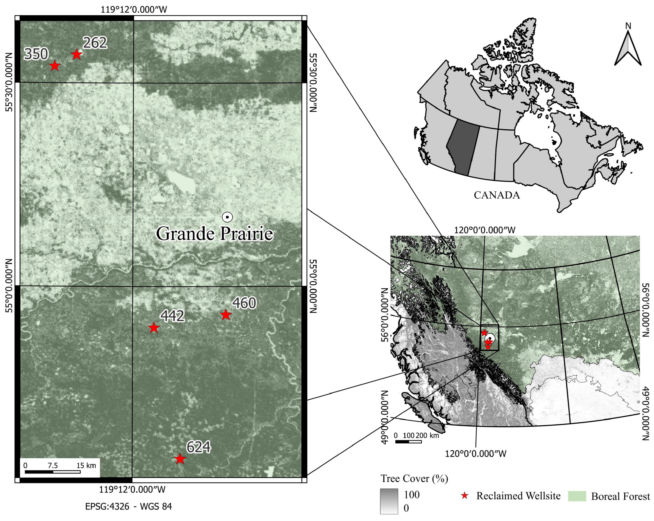
The study area was located near Grande Prairie in northwestern Alberta, Canada (Figure 1). This region has been a hub for oil and gas extraction and forestry since the 1950s, leading to the development of numerous wellsites throughout the surrounding forested areas. Mean daily temperature normals in this region range from −14 °C in January to 16 °C in July, and mean monthly precipitation normals range from 16 mm in February to 73 mm in July [32].
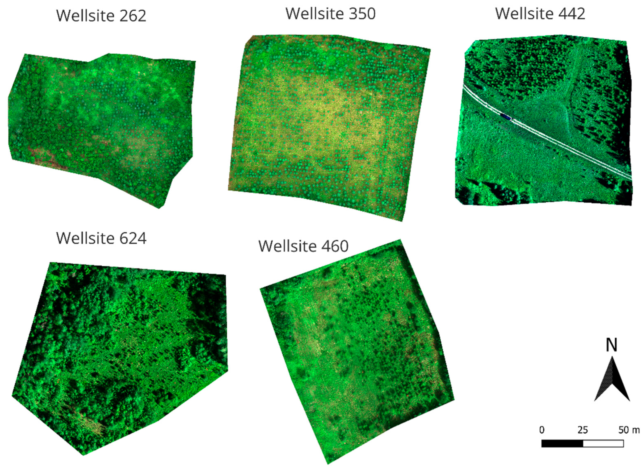
Five certified reclaimed wellsites were selected for this study (Table 1). Two wellsites (442 and 460) are located in Alberta’s Central Mixedwood natural subregion, and three wellsites (350, 262, and 624) are situated in the Lower Foothills subregion [35]. The Central Mixedwood subregion is characterized by mixedwood stands dominated by aspen in early successional stages and white spruce at later stages, with elevation ranging from 200 to 1050 m. The Lower Foothills subregion is a diverse region characterized by mixed stands of aspen, lodgepole pine, white spruce, and balsam poplar with elevation ranging from 650 to 1625 m [35]. Each wellsite measured approximately 100 × 100 m and was reclaimed to the 1995 Reclamation Criteria for Wellsites and Associated Facilities [36]. Between 2006 and 2009, sites were planted with either Picea glauca (white spruce) or Pinus contorta (lodgepole pine) by Weyerhaeuser (Figure A1). Naturally regenerating Populus balsamifera (balsam poplar) and Salix sp. (willow) were also present throughout many of the wellsites. Tree heights, densities, and species composition varied across the five sites (Table 1), with additional variation in species and densities observed within individual wellsite.

2.2. Data Acquisition and Preparation

UAV-LiDAR and MS imagery were collected at each wellsite over three field campaigns conducted in August 2023, October 2023, and May 2024, capturing data under summer (leaf-on), autumn (deciduous: fully leaf-off), and spring (early leaf development phase) conditions. We excluded snow-cover periods because they substantially affect RS performance and require specialized processing beyond the scope of this study. Before each data acquisition, five ground control points (GCPs) were set at the corners and middle of the wellsite using a Trimble DA2 global navigation satellite system (GNSS) receiver with a Trimble Catalyst 10 Subscription that provides 10 cm accuracy.

2.2.1. UAV-LiDAR Data

LiDAR data were collected using a DJI Zenmuse L1 sensor (SZ DJI Technology Co., Ltd., Shenzhen, China) mounted to a remote-controlled quadcopter DJI Matrice 300 RTK (SZ DJI Technology Co., Ltd., Shenzhen, China). The flight altitude for all missions was set to 50 m and the flight speed to 5 m s−1. A triple signal return mode and 70% side and 70% forward overlap were used, resulting in high-density point clouds (an average point density of 1159 points m−2) with 1.36 cm ground sample distance (GSD). The L1 sensor is also equipped with a 24 mm RGB mapping camera with 1-inch CMOS 20 MP sensor (SZ DJI Technology Co., Ltd., Shenzhen, China) to colorize the point cloud, providing additional RGB data along with the point cloud data for the model to use in tree detection, segmentation, and classification. A DJI D-RTK 2 GNSS Mobile Station (SZ DJI Technology Co., Ltd., Shenzhen, China) was used for georeferencing the datasets. To improve spatial accuracy, a stationary Trimble R8 GNSS (Trimble Inc., Sunnyvale, CA, USA) receiver was used to provide data for Precise Point Positioning (PPP) correction [37]. DJI Terra Pro v.4.2 (SZ DJI Technology Co., Ltd., Shenzhen, China) software was used for final point cloud reconstruction stitched with the RGB color from into a LAS file [38].

2.2.2. Aerial MS Data

A MicaSense RedEdge-P (MicaSense, Inc., Seattle, DC, USA) MS sensor mounted to the same quadcopter DJI Matrice 300 RTK (SZ DJI Technology Co., Ltd., Shenzhen, China) was used to acquire MS images from a second flight over each wellsite. The sensor captures images in five spectral bands [39] with a focal length of 5.5 mm and a horizontal field of view of 49.6°. With a flight altitude of 50 m, this sensor provided a GSD of 3.3 cm/pixel per each spectral band. A Downwelling Light Sensor 2 (MicaSense, Inc., Seattle, DC, USA) was calibrated before each flight and deployed along with the sensor to improve reflectance calibration in situations where ambient light conditions were changing in the middle of a flight. To calibrate the reflectance values of the camera, a picture of the MicaSense calibrated reflectance panel (MicaSense, Inc., Seattle, DC, USA) was captured before and after each mission. Pix4Dmapper v4.8.4 (Pix4D, Lausanne, Switzerland) software was used to process the acquired images into orthophotos. The post-processing workflow included the following: (1) key point identification, bundle adjustment, and image pair matching; (2) geometric correction using GCPs; (3) point cloud generation and 3D textured mesh creation; (4) radiometric processing and calibration using calibration reflectance panels (CRPs); and (5) generation of the digital surface model and orthomosaic. The resulting five separate radiometrically corrected orthomosaics, one for each spectral band were exported. Using QGIS v.3.34.10 (Grüt, Switzerland) software, the exported images were then bonded into multilayer orthomosaics for further processing.

2.2.3. LiDAR and MS Data Fusion

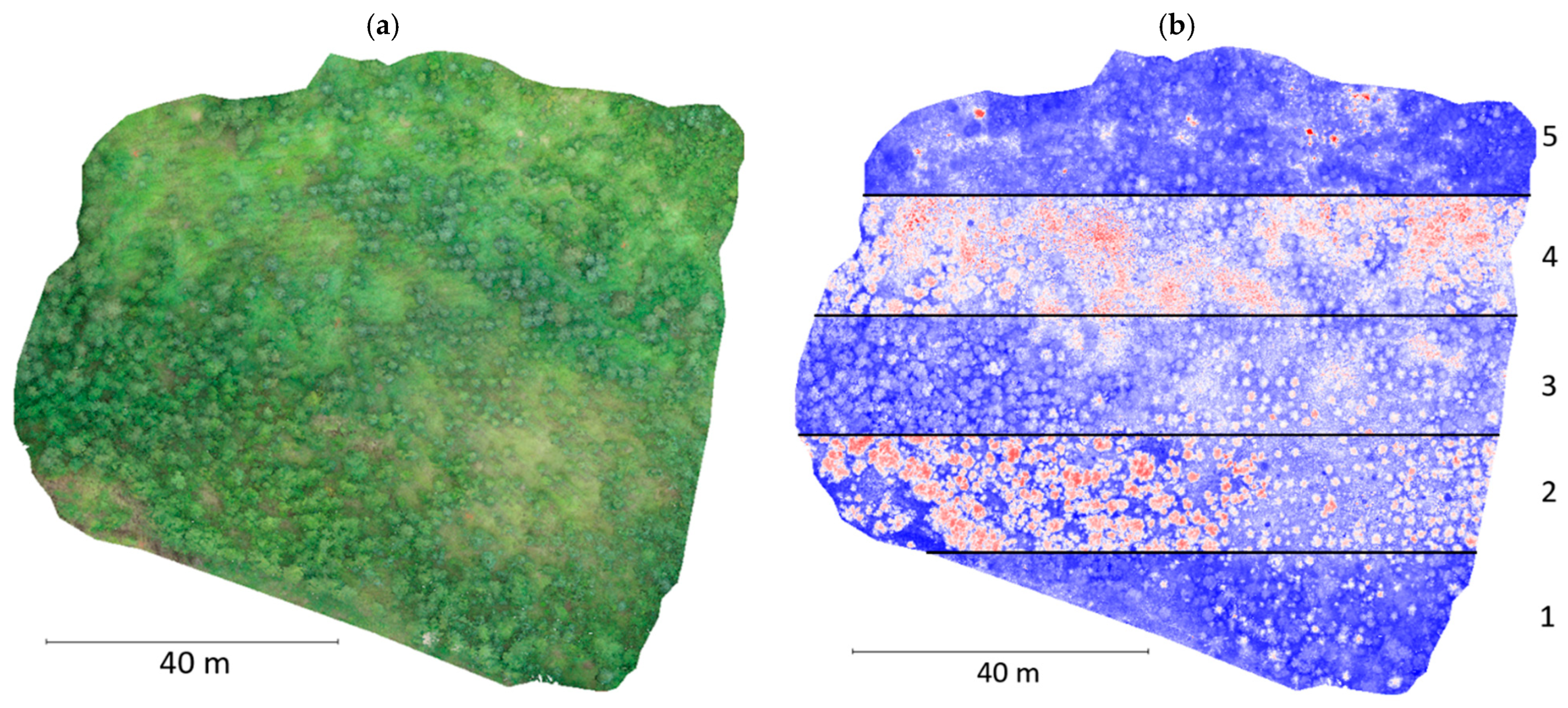
The data fusion process requires that raster and point cloud datasets be co-registered with high accuracy for subsequent 3D voxel-level DL. First, RGB point clouds generated by DJI Terra Pro v.4.2 (SZ DJI Technology Co., Ltd., Shenzhen, China) were projected into 2D rasters. Corresponding points between these rasters and the MS orthomosaic rasters were manually identified and paired in QGIS v.3.34.10 (Grüt, Switzerland). Using those control points, we applied a Thin Plate Spline (TPS) algorithm [40] to warp the orthomosaic. The resulting aligned five-band pixel values were then mapped back onto the 3D point cloud as additional attributes (see Figure A2) using Rasterio v.1.4.3 [41] and laspy v.2.5.0 [42] python libraries.

2.2.4. Field Data for Model Validation

To validate the models, we collected reference tree data across each wellsite concurrently with the RS data acquisition, creating a validation dataset of individual-tree heights and locations. In total, 342 reference trees were sampled: 84 white spruces, 78 lodgepole pines, 55 balsam poplars, and 125 willows (Table 1). For each reference tree, tree species was identified, tree height was measured using a tree height pole, and tree location was recorded using the Trimble DA2 (Trimble Inc., Sunnyvale, CA, USA) GNSS receiver.

3. Methodology

3.1. Workflow Description

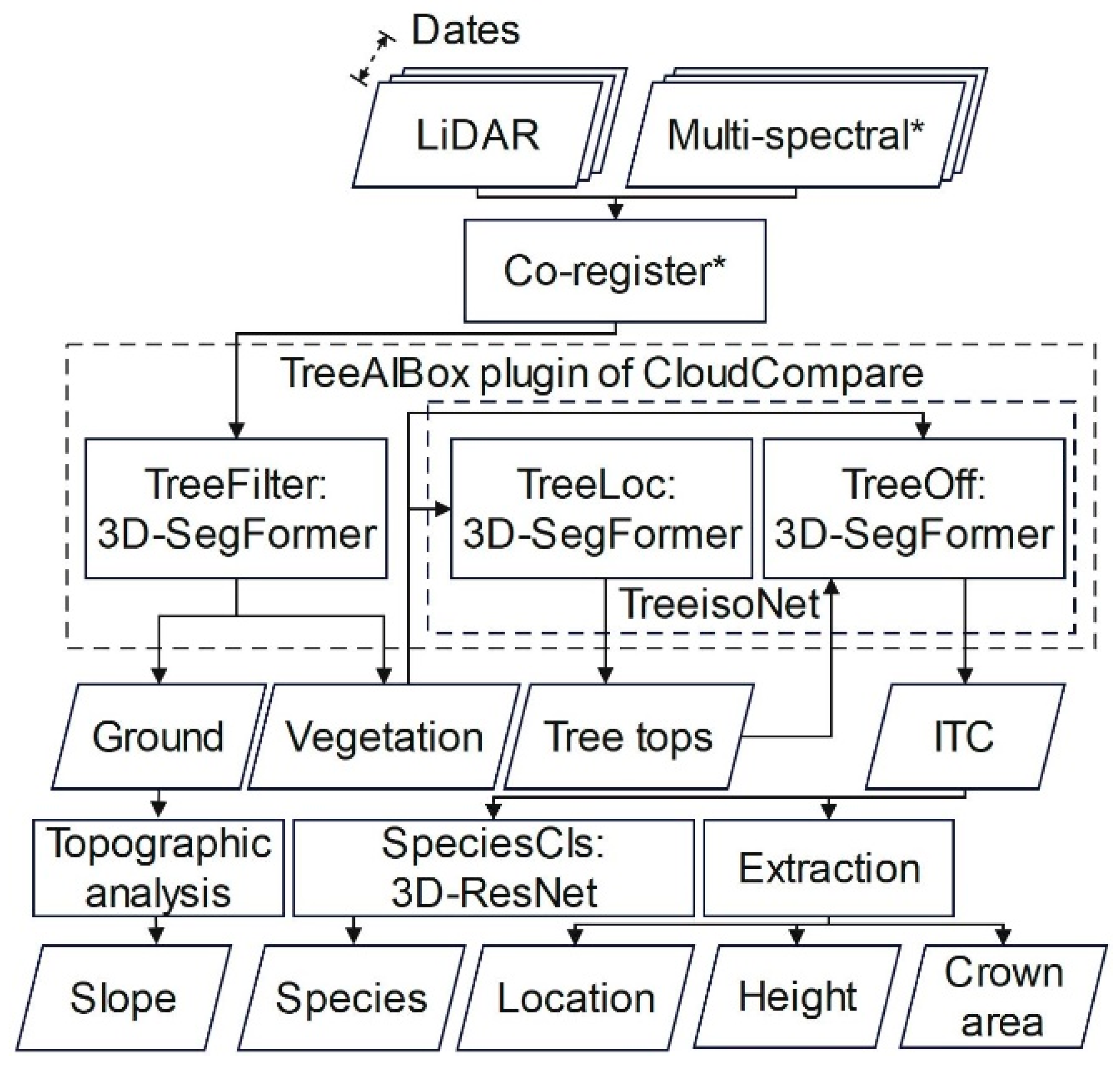
The UAV-based workflow for extracting vegetation statistics from reclaimed wellsites is illustrated in Figure 2. The process began with co-registration of a LiDAR point cloud and MS image using thin plate spline interpolation in QGIS. The resulting MS point cloud, stored in LAZ format, included five MS bands as additional attributes [38]. Four DL models were used (Figure 3): (1) TreeFilter: 3D-SegFormer for separating vegetation [43]; (2) TreeLoc: 3D-SegFormer producing 2D tree top locations, adapted from [44]; (3) TreeOff: 3D-SegFormer for individual tree segmentation, adapted from [44]; and (4) SpeciesCls: 3D-ResNet for classification of individual tree species as either coniferous or deciduous [45]. The first three models are implemented in the CloudCompare software v.2.14 as a graphical user interface plugin, TreeAIBox (https://github.com/NRCan/TreeAIBox (accessed on 1 October 2025)).
Compared to our previously described methodology [44], TreeAIBox replaces 3D-UNet with 3D-SegFormer for conceptual consistency. SegFormer was optimized with skip-fusion, reducing GPU demand and enabling larger voxel blocks (1283). This architecture combines transformer-based long-range encoding with efficient multi-scale feature extraction, outperforming alternatives such as 3D-UNet which requires more memory and has a smaller receptive field, while PointNet++ struggles to delineate crown boundaries in dense LiDAR data. Given the very high point density (1159 points m−2), voxelized SegFormer provided an effective balance between geometric fidelity and computational efficiency.
This TreeAIBox workflow starts by separating vegetation (class 2) from non-vegetation (class 1), enabling generation of a 1 m2 digital terrain model (DTM) and slope maps through lowest non-vegetation one-point filtering and grid interpolation. Next, TreeLoc identifies treetop locations for individual trees using confidence and radius predictions and generates a point cloud layer of detected treetops. TreeOff then extracts individual tree characteristics (ITC): location, height (vertical difference between highest point of tree and corresponding DTM elevation), and crown area (area of the 2D convex hull enclosing the tree points). After which, SpeciesCls classifies each tree as deciduous or coniferous. Species-level identification is not required for reclamation assessment, which only tracks woody stem density [9], but distinguishing between coniferous and deciduous species provides insights into the survival of planted trees. This study applied the workflow to reclaimed wellsites rather than focusing on further methodological development.

3.2. Model Training and Accuracy Assessment

To meet GPU memory constraints, the LiDAR point cloud was divided into blocks and voxelized. The voxel dimensions were customized to balance the preservation of fine structural detail with feasible training on a single GPU (Table 2). For example, the TreeOff model used voxels of 10 cm × 10 cm × 20 cm, which were sufficient to capture branch-level detail and crown boundaries while keeping memory requirements manageable for 1283 blocks. The chosen dimensions are consistent with previous UAV-LiDAR segmentation studies and represent an optimal trade-off between accuracy and efficiency. Binary voxel values (0 = empty, 1 = occupied) were used for TreeFilter, TreeLoc, and SpeciesCls with additional MS information averaged and attributed to each voxel. For TreeOff, binary tree top location voxels were also included as additional dimensions, extending the input to, e.g., 128 × 128 × 128 × 7 with five spectral bands (Figure 3).
Reference data were manually labeled for vegetation, treetop locations, individual-tree IDs, and species (1 = coniferous, 2 = deciduous). These annotations were split into training and testing sets (Table 2), keeping the split area continuous to minimize sampling bias. Data augmentation was limited to random rotation and window-based cropping, which directly address the primary sources of variability in canopy orientation and crown arrangement. These methods effectively increase geometric diversity without altering the physical realism of the LiDAR and MS signals. Intensity or brightness augmentation was deliberately avoided because LiDAR intensity and MS reflectance values are physically calibrated quantities and artificially modifying them could reduce data reliability. While future work may explore more advanced augmentation strategies, geometric augmentation was prioritized as it provided the greatest impact on tree segmentation accuracy.
Training minimized the prediction error against the reference labels using the AdamW optimizer [46], with checkpoints saved for the models achieving the highest testing accuracy. For inference, a trained model was applied in overlapping blocks across the entire study area, and block-level predictions were fused into the final output. Accuracies were quantified using four metrics: (1) TreeFilter: mean intersection over union (mIoU) for vegetation and non-vegetation classes; (2) TreeLoc: precision, recall, and F1-score for tree top detection; (3) TreeOff: mIoU for individual tree instances; and (4) SpeciesCls: mIoU across coniferous and deciduous classes. Precision was defined as the number of reference tree crowns with exactly one model predicted treetop divided by the total number of model predictions. Recall was defined as the number of model-predicted treetops with exactly one reference tree crown within their radius, divided by the total number of reference trees. The F1 score was calculated using F1 = 2 × (Precision × Recall) ÷ (Precision + Recall).

3.3. Model Evaluation and Application

The workflow described in Section 3.1 and Section 3.2 was implemented with data from five wellsites with different spectral bands collected across different seasons. To assess the impact of additional spectral bands on model performance, we evaluated our algorithm under three scenarios: (1) LiDAR point cloud only, (2) LiDAR point cloud + RGB band (from the DJI Zenmuse L1), and (3) LiDAR point cloud + five MS bands (including RGB, NIR, and red edge) for training and testing. Next, we used the LiDAR + RGB data to evaluate the accuracy of height measurements and detection rates of reference trees. The field-measured, geolocated trees served as references and were manually matched by visual inspection of the delineated trees in the point clouds based on spatial proximity. The detection rate was defined as the number of matched trees divided by the total number of reference trees, and the heights of the matched trees were validated by comparing with field-measured heights. Next, we explored the various detection and classification errors and how these were affected by tree height, site, and species. To assess the repeatability and consistency of this method, we evaluated the algorithm using RS data collected across different seasons: summer, autumn, and spring. To balance processing efficiency and data volume, we used LiDAR-only models for individual-tree delineation and LiDAR + RGB models for classification. Since species classification was unreliable for low vegetation, trees shorter than 1 m were classified as part of the shrub layer, resulting in three classification groups: deciduous, coniferous, and shrub. Both model sets were re-trained on the complete reference dataset (training + testing) for wellsite monitoring.

4. Results

4.1. Effect of Additional Spectral Data on Model Accuracy

Testing accuracies of the LiDAR point cloud, LiDAR + RGB, and LiDAR + MS are summarized in Table 3 and visualized in Figure 4. Across the five wellsites, the average mIoU was 0.93 for TreeFilter, the average F1-score was 0.83 for TreeLoc, and the average mIoU was 0.83 for TreeOff for LiDAR point cloud data only. Incorporating RGB or MS bands did not significantly improve the accuracy of these modules. However, classification showed notable gains: the mean mIoU increased from 0.78 with LiDAR alone to 0.84 with the addition of RGB bands, and further to 0.88 when the full MS dataset was incorporated. Under the MS scenario, deciduous species (Pb and Sx) had a mean mIoU of 0.82, while conifer species (Pl and Sw) achieved a higher mean mIoU of 0.93.
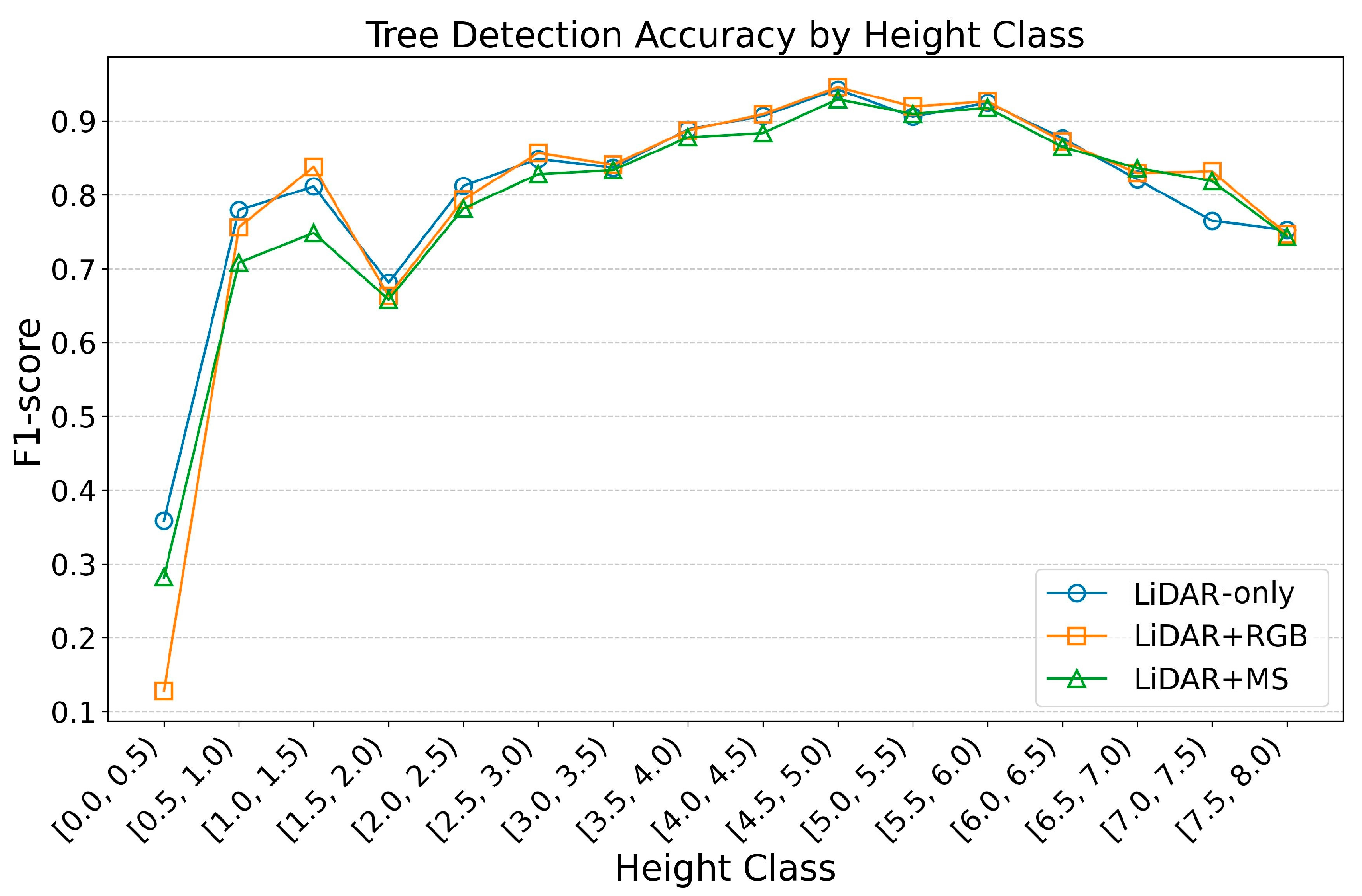
Tree-detection F1-scores across height classes for the different datasets are shown in Figure 5. Detection accuracy does not improve for either short or tall trees when additional bands are included.

4.2. Validation of LiDAR-Derived Heights and Detection Rates with Reference Trees

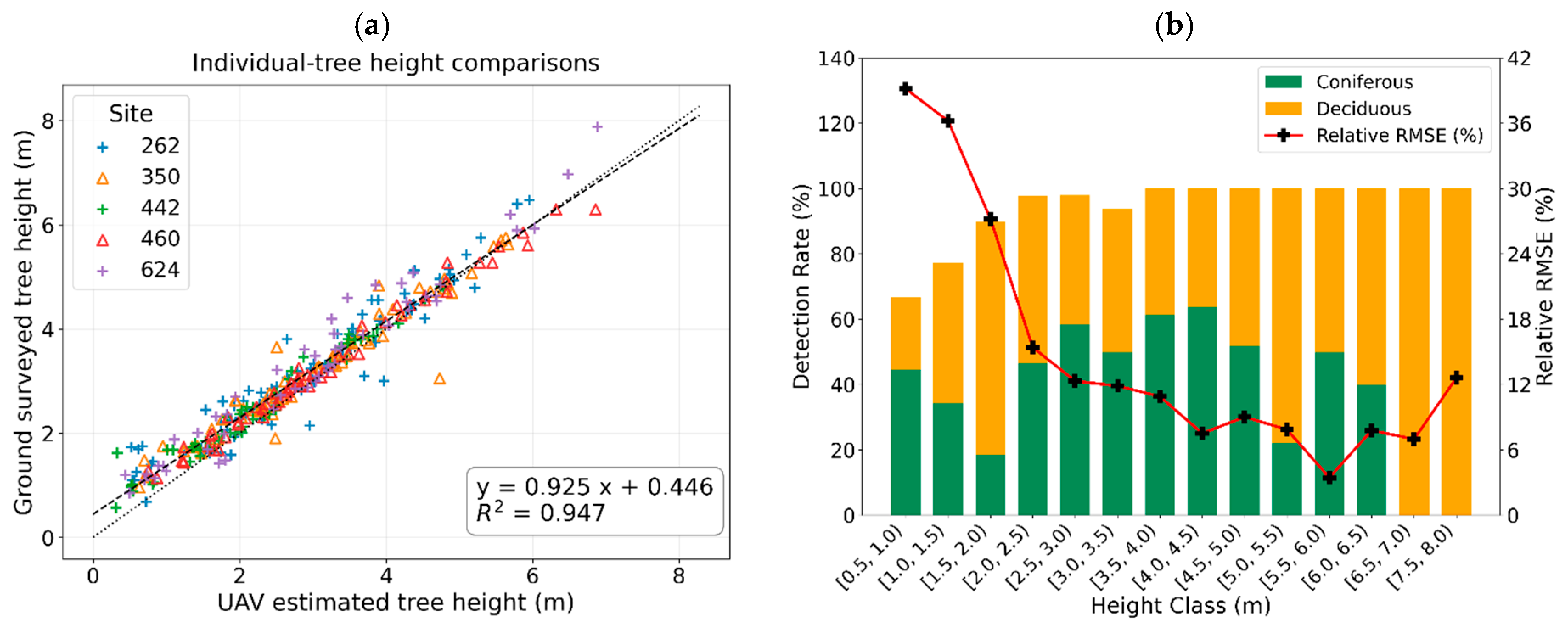
The following results are from the LiDAR point data only. Of the 342 geolocated reference trees, 93.8% (321 trees) were matched to LiDAR-detected individuals. Using field measurements as reference, LiDAR-derived heights yielded an RMSE of 0.40 m (12.9% RMSE%) (Figure 6a), with a strong correlation (R2 = 0.95). Figure 6b presents the height-error distribution and detection rate by height class. RMSE% was highest (>39%) for trees < 1 m, decreased to < 10% for trees between 4 and 7 m, and rose slightly above 12% for trees > 7 m. Detection rate was 93% for trees between 1.5 and 2 m, and exceeded 95% for trees taller than 2 m, but dropped to 77% for trees between 1 and 1.5 m, and to 67% for trees < 1 m.

4.3. LiDAR Error Sources

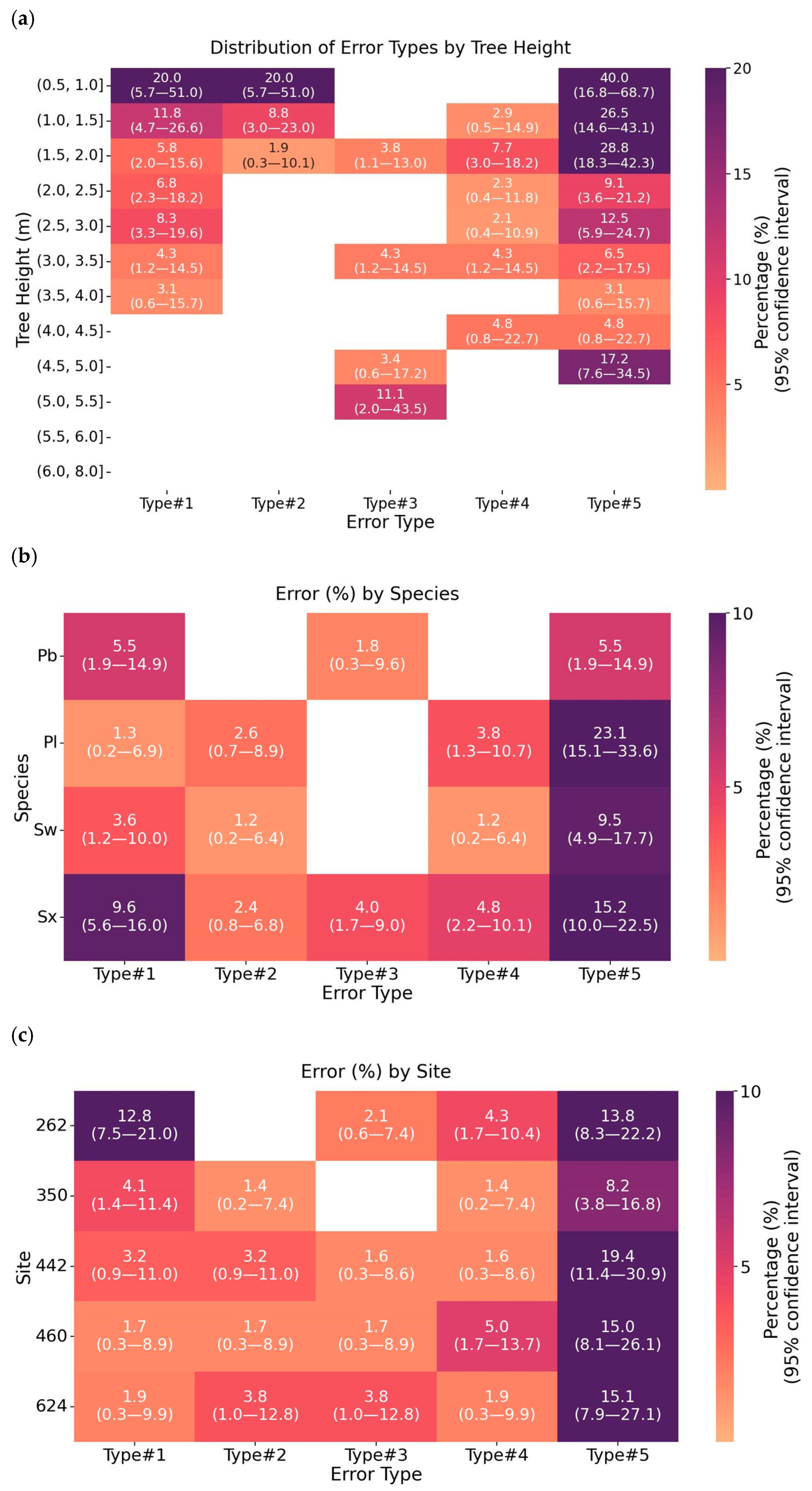
Tree locations extracted by TreeOff were compared with reference tree data, allowing evaluations of detection and classification accuracy on a per-tree basis using LiDAR data. Five types of error sources for tree detection were identified: (1) invalid field data: errors due to incorrect geolocation (e.g., no corresponding tall trees in the point cloud); (2) TreeFilter misses: occlusion, or sparse/low-density points, resulting in unfiltered (undetected) trees; (3) over-detection: single tree split into multiple instances by TreeLoc and TreeOff; (4) under-detection: neighboring trees merged due to detection and segmentation errors by TreeLoc and TreeOff; and (5) misclassification: incorrect classification predictions (for trees without the above four error types).
The proportions of these five error types varied among height class, species, and site (Figure 7). Geolocation errors occurred across all height classes but generally decreased with increasing tree height (Figure 7a). No geolocation errors were observed for trees taller than 4 m. TreeFilter misses were most frequent in short trees (<2 m), affecting up to 20% of trees under 1 m. Short trees were rarely over-detected, with the highest rate (11%) occurring in the 5.0 to 5.5 m class. Under-detection was more evenly distributed between 1 and 4.5 m and was more common overall than over-detection.
When separated by species (Figure 7b), all five error types appeared in willow. Error rates varied more by species than by the deciduous vs. coniferous grouping. For example, balsam poplar showed few instances of error type #2 to #4 compared to conifers (Figure 7b). Wider-crowned broadleaf species such as willow and poplar often have irregular or dome-shaped crowns, causing the detected apex to be offset from the true stem location, whereas narrow, conical crowns of species like lodgepole pine align more closely with the stem, resulting in smaller geolocation errors. All five error types occurred across the different sites, with less site-specific variation than seen among species (Figure 7c).
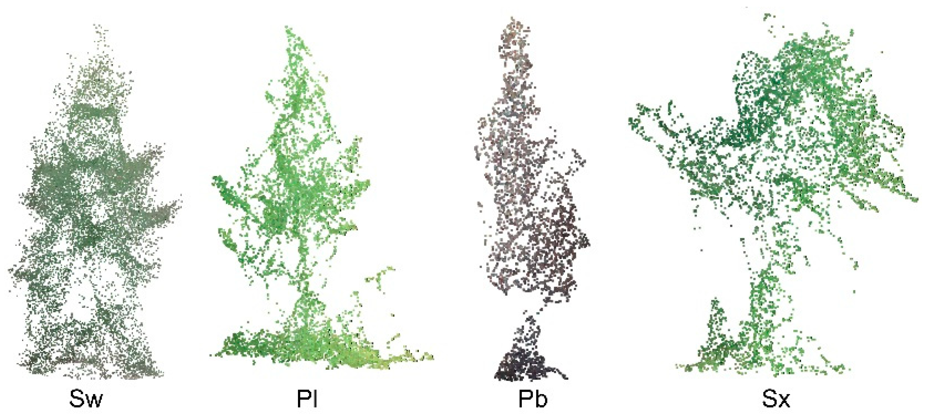
For misclassification (type 5), small trees posed the greatest challenge with more than 25% of trees under 2 m misclassified (Figure 7a). When plants are young, their morphological traits are not yet distinct enough for reliable differentiation: young lodgepole pine, and white spruce all exhibit similarly conical shapes in the point cloud (Figure 8), leading to lower classification accuracy (Figure 7a).

4.4. Capturing Seasonal Changes for Wellsites Monitoring

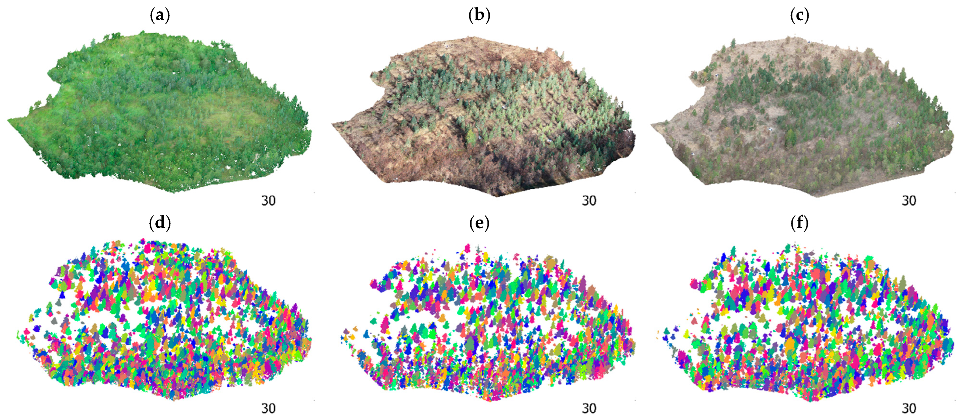
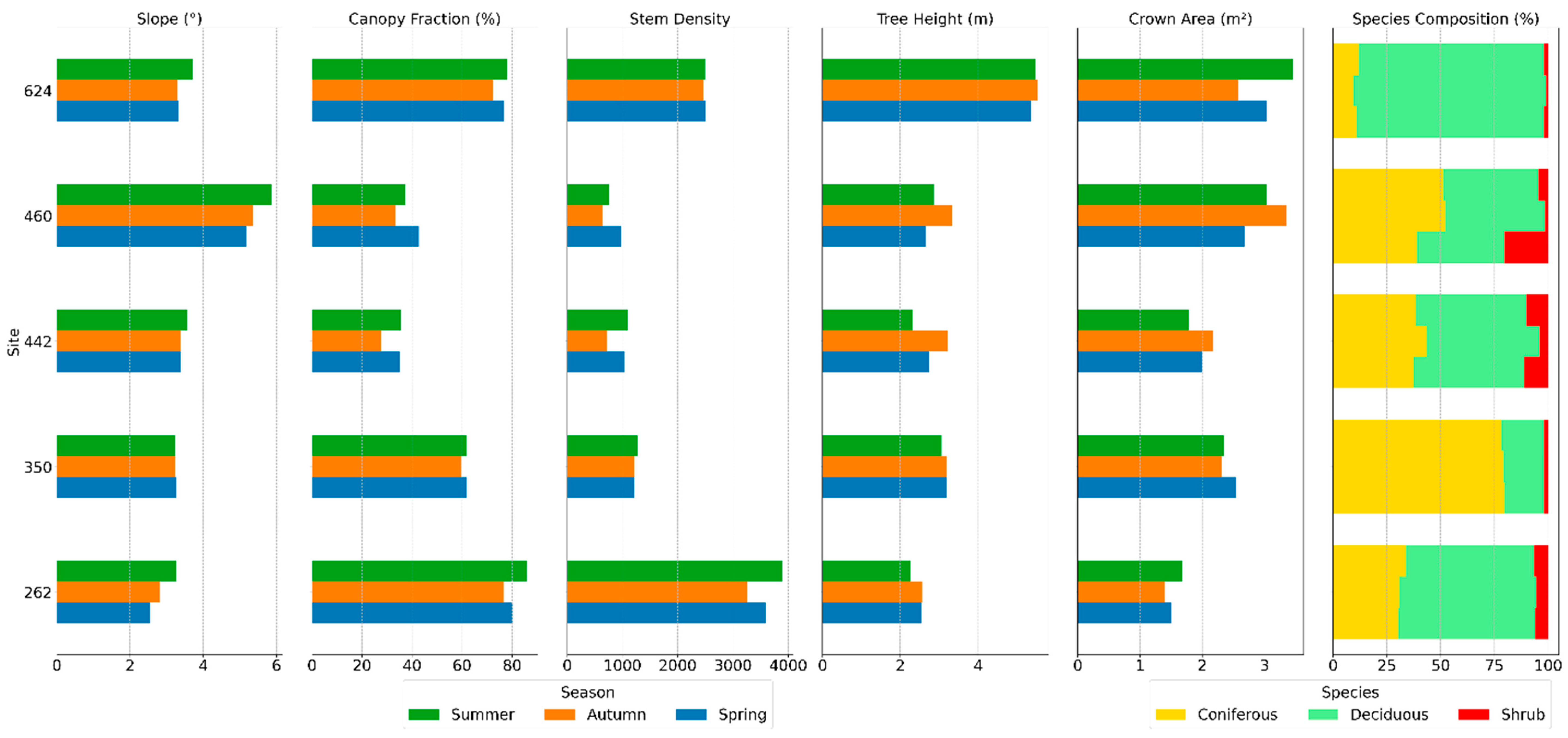
The TreeAIBox models extracted similar terrain and individual tree metrics using site data from different seasons (Figure 9). An example of extracted individual trees from a wellsite across the three seasons is shown in Figure A3. Terrain slope remained consistent across time points, with a variation of ±1°, indicating reliable ground filtering and consistent data acquisition. Canopy fraction decreased in autumn from abscission at all sites except wellsite #460, where a dense spring shrub layer contributed to a higher spring canopy fraction earlier in the season (Figure 9). Mean tree height generally increased from spring to autumn. However, wellsites #442, 350, and 262 showed a drop in mean height in the summer, likely due to the recruitment of numerous small stems, which lowered mean height and reduced crown area. In contrast, wellsite #624, which had a more mature stand and stable stem density, showed a peak in crown area during the summer, aligning with expected seasonal growth pattern. These findings demonstrated that mean height alone does not fully capture the complexity of vegetation change at the site level. They also highlight the value of RS data, which complement ground plots by providing a broader, site-wide perspective on vegetation structure and species composition.
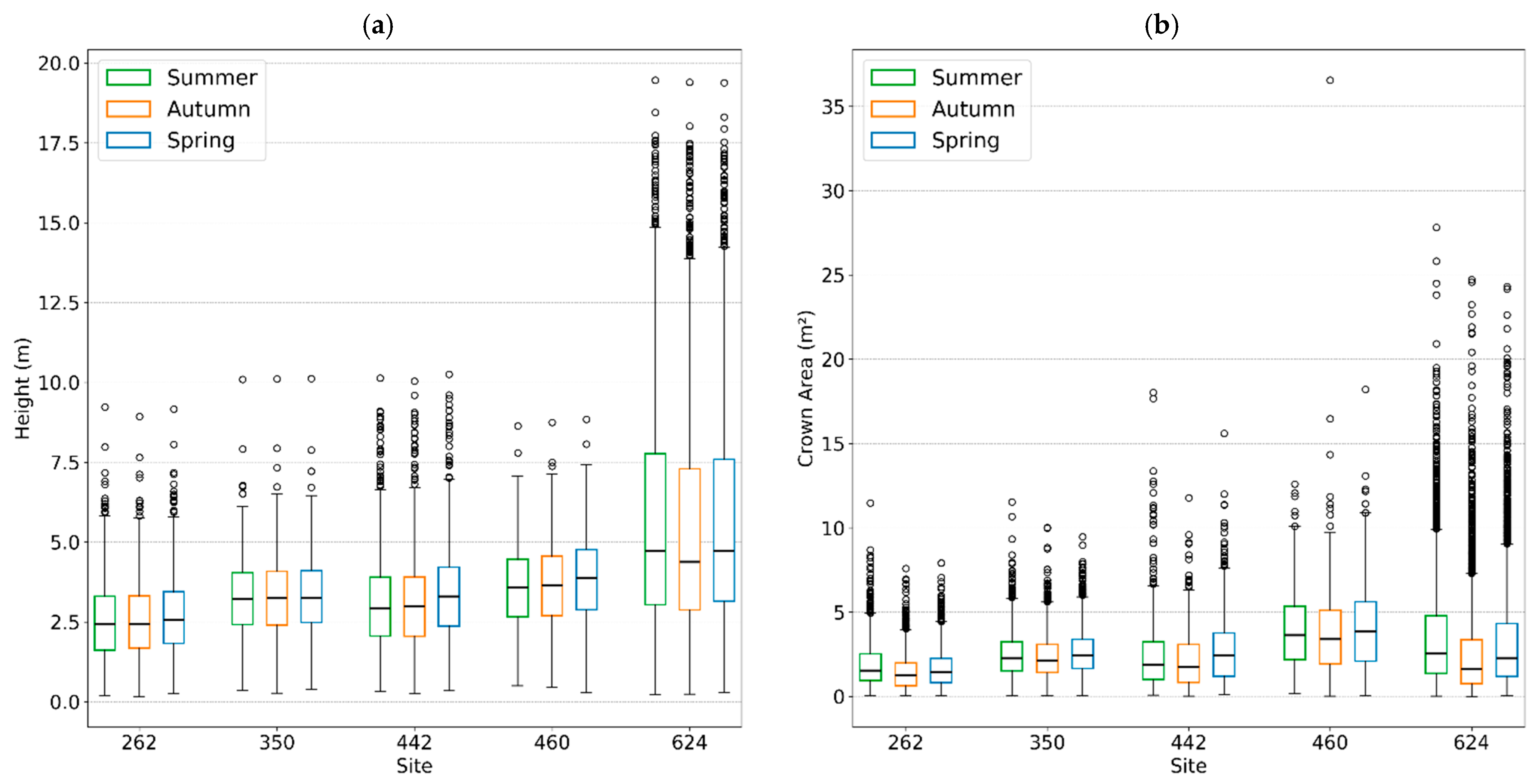
Tracking the same trees over time allows for the separation of individual-tree growth from changes in overall tree count. Based on median values, tree height increased by 0.3% from summer to autumn and by 3.6% from autumn to the following spring (Figure 10a). Crown area decreased by 8.5% between summer and autumn, then increased by 15.2% from autumn and spring (Figure 10b). These results highlight the workflow’s ability to detect subtle changes in height and crown area, supporting its utility for long-term vegetation monitoring, affirming that UAV surveys can offer a reliable approach for continuous, tree-level monitoring at wellsites.
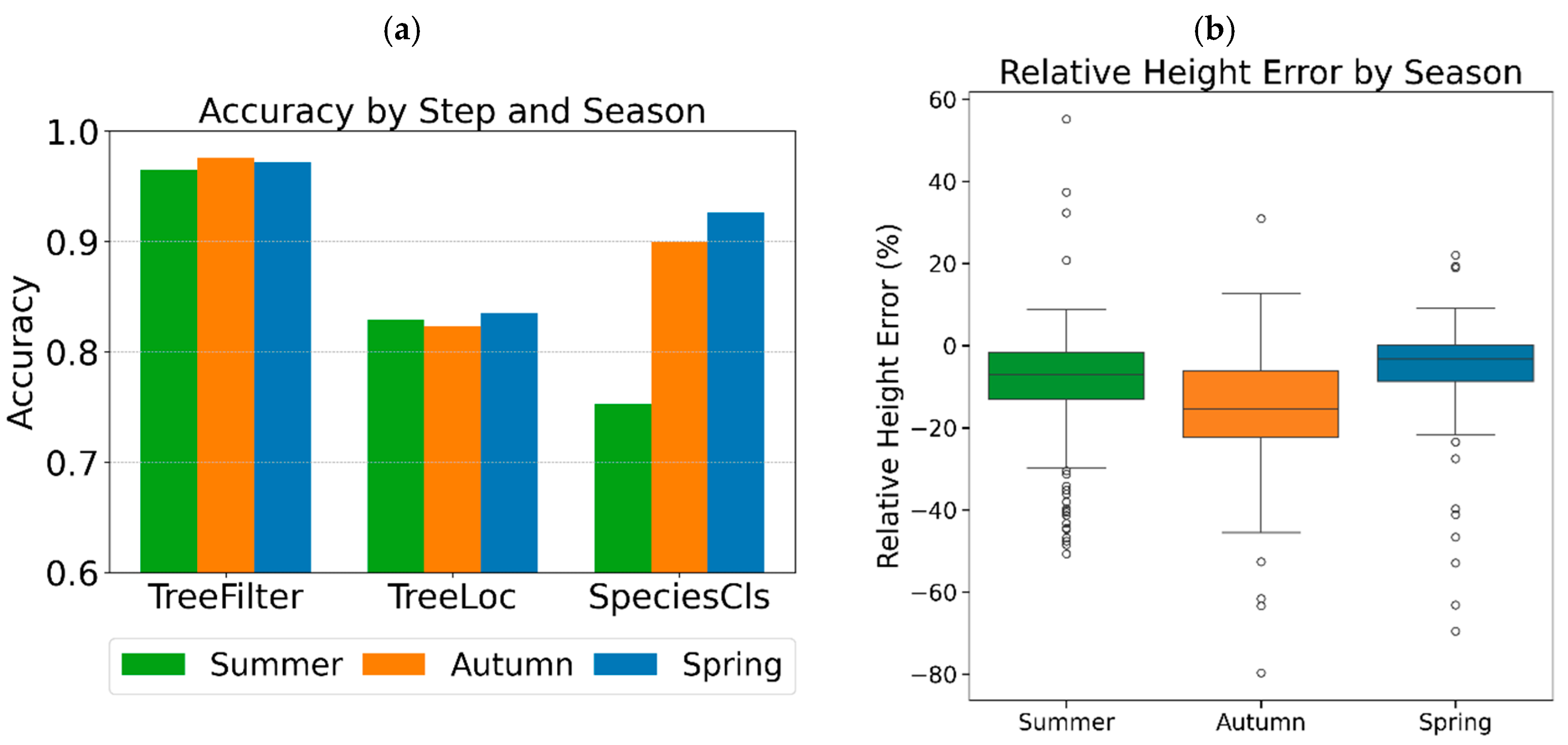
Seasonal accuracy for each module: TreeFilter and TreeLoc (using LiDAR-only data) and SpeciesCIs (using LiDAR + RGB data) are shown in Figure 11a. While TreeFilter and TreeLoc maintain consistent performance across all seasons, the accuracy of the SpeciesCIs module drops to 0.75 in summer, compared to 0.93 in spring and 0.90 in autumn. Additionally, spring showed the lowest variability in relative height error (Figure 11b).

5. Discussion

5.1. Challenges in Short Tree Detection and Height Estimation

Detecting and accurately measuring the height of short trees, particularly those under 2 m tall, remains to be one of the persistent challenges in using UAV-LiDAR systems. In our study, we experienced significant difficulties in filtering and delineating these shorter trees, resulting in a consistent underestimation of their heights. This challenge aligns with findings from Rodríguez-Puerta et al. [47] and Pearse et al. [20], who also reported reduced accuracy in detecting small trees (< 1 m tall) in structurally complex forest environment using UAV-LiDAR and imagery. Similarly, Xiang et al. [13] observed a notable decline in understory tree detection accuracy with F1-score dropping from 82.9% for dominant trees to 39.3% for understory trees.
The challenge of small tree detection is rooted in sensor limitations and methodological constraints. UAV-LiDAR systems often generate fewer returns near the forest floor due to canopy occlusion, which results in sparse ground and understory point distributions [13,47,48]. These conditions make it particularly difficult to differentiate between low vegetation, ground clutter, and actual tree structures. Also, short trees, especially coniferous saplings, often possess fine leaders that are difficult to capture in LiDAR point clouds due to their small cross-sectional area and lower reflectance [49,50]. These fine-scale features frequently fall below the spatial resolution threshold necessary for reliable detection. Additionally, terrain roughness and tall herbaceous vegetation can exacerbate detection difficulties [20]. In our analysis of five wellsites, we measured a ground-layer “thickness”, defined as the mean elevation deviation between classified ground returns and the DTM grid of 10 to 15 cm. This ground surface variation introduces further uncertainty in identifying and measuring the vertical extent of short trees. All these factors also make it more difficult to annotate small trees for training datasets, resulting in a bias in filtering and segmentation algorithms toward mid- to large-sized trees [13]. Together, these factors make the algorithms less effective at identifying and accurately extracting the features of short vegetation. Hamraz et al. [51] found that even with eleven customized DL and machine learning architectures, detecting understory conifers remained poor, the limiting factors being data quality and the indistinct geometry of small trees, not the algorithms themselves.
In the reclamation monitoring context, short trees and shrubs often represent early successional recovery and contribute disproportionately to canopy cover metrics required for certification. Under-detection of these stems could lead to underestimated vegetation recovery status. Understanding and explicitly accounting for these sources of error is thus critical to ensuring that UAV-based monitoring tools can be applied reliably in regulatory and management contexts.

5.2. Impact of Spectral and Geometric Domains on ITD and Classification

Our results revealed that the treetop detection module (TreeLoc) performed robustly across all three data scenarios (LiDAR points only, LiDAR + RGB, and LiDAR + five MS bands) (F1  >  0.80; Table 3, Figure 4), indicating that adding spectral information yields minimal improvement in tree detection rate. This finding contrasts with Dai et al. [30], who reported a 7% gain in tree detection by adding spectral bands to low-density 3D point clouds (~58 points m−2). We attribute this discrepancy to point density; our LiDAR datasets average 1159 points m−2, a level at which 3D spatial information alone appears sufficient for accurate detection. Recent studies further support this theory, showing that DL models maintain stable ITD performance above 100 points m−2 while detection quality deteriorates sharply below 50 points m−2 due to increased omission errors [12,48]. Hao et al. [27] found that adding extra spectral bands to RGB can negatively affect Mask R-CNN-based ITD, whereas Mao et al. [28] reported that including the NIR band markedly improves detection relative to other bands. These mixed findings suggest that the benefits of spectral information depend on site, species, and scene context.
Despite minimal improvements in tree detection rates, adding spectral variables to geometric structural information resulted in a noticeable increase in accuracy for the classification module (SpeciesCls) to separate coniferous and deciduous trees. Additional spectral information enhanced model accuracy from 78% (for LiDAR point only) to 84% and 88% for LiDAR + RGB and LiDAR + five MS bands datasets, respectively (Table 3, Figure 4). This finding demonstrates that spectral cues, especially NIR and red-edge bands, provide important complementary information for distinguishing between coniferous and deciduous trees. These results are consistent with Waser et al. [52] who also showed that adding RGB and NIR spectral bands substantially enhances classification performance compared to geometric variables alone. Despite the improved performance, the model’s classification accuracy for deciduous species remains below 90%. This underperformance may be attributed to several factors: (1) high inter-individual variability in young deciduous trees, (2) lower reflectance stability across phenological stages [53], and (3) class imbalance in the training dataset.
Height-stratified analysis revealed that classification performance declined with tree height below 2 m. For these smaller individuals, the shapes of young spruce, pine, and willow overlap in 3D structure, leading to misclassification. This indicates that, in addition to adding spectral information, improving detection of short trees and their structural representation is essential to enhance classification. Willows also exhibited high morphological variability due to their irregular multi-stemmed forms. These traits increased omission errors and species confusion, highlighting the challenge of applying individual tree-based methods to shrubby, morphologically variable forms.
Several potential solutions may mitigate the challenges associated with small tree and irregular-tree-form detection and classification. Future studies should explore increasing LiDAR point density or combining multiple flight altitudes could enhance penetration into the understory. Multi-resolution feature learning architectures may better capture coarse crown structure and fine understory geometry. Context-aware learning modules, which use spatial context to differentiate shrubs from trees, also hold promise. From a data perspective, systematic annotation of small trees and deciduous species, including crown boundaries and multi-stem growth forms will be essential to reduce bias in future training datasets.

5.3. Season Selection for UAV Survey of Trees on Wellsites

Models trained on summer and autumn data maintained high accuracy when predicting spring condition datasets (Table 2 and Table 3), demonstrating strong seasonal adaptability, an essential trait for monitoring reclaimed wellsites, where foliage cover changes throughout the year and consistent tree detection is critical for evaluating reclamation success and ecological recovery.
An important consideration in interpreting seasonal results is the potential influence of measurement artifacts. For example, the apparent 3.6% increase in median tree height from autumn to spring may reflect early spring flush adding height, rather than true winter biomass accumulation. Similarly, seasonal differences in crown area may partly reflect changes in foliage density and LiDAR penetration rather than actual structural change. These artifacts highlight the importance of cautious interpretation when monitoring across phenological phases.
Although tree detection rates remained consistent across seasons, the precision of structural features and spectral signatures necessary for reliable classification and growth tracking was season-dependent. Ecological and phenological factors also explain much of the seasonal variability in classification accuracy. Spring conditions yielded the highest classification accuracy (mIoU = 0.93), likely because reduced leaf cover improves visibility of the apical meristem, branching patterns, and crown geometry, which are important cues for classification. Conversely, summer performance was lower (mIoU = 0.75), probably due to dense foliage obscuring structural traits, despite the expectation of strong spectral separability under full leaf-on conditions. Autumn provided an intermediate case (mIoU = 0.90), where partial leaf-off improved geometry capture but spectral variability from senescing foliage introduced additional noise. These results underscore the need to align survey timing with phenological windows that optimize both structural and spectral separability for tree monitoring tasks. Moreover, metrics such as relative height error were lowest in spring (Figure 11b), indicating that spring provided the clearest point cloud representations for accurate height estimation and may be the most suitable time of the year for conducting UAV-LiDAR tree surveys in wellsite monitoring, at least under these experimental conditions.

5.4. Study Limitations

Results from this study demonstrate that UAV-based DL can deliver reliable site-wide measurements of vegetation recovery, while also exposing challenges unique to reclaimed wellsites. The reclaimed wellsites in this study were mixed stands dominated by either white spruce or lodgepole pine from within the Central Mixedwood and Lower Foothills natural subregions of Alberta 14 to 18 years post-planting. Hence, the application of our methods is limited to these stand types and ages. However, in Alberta, approximately 68% of the province is forested with the Central Mixedwood subregion and Lower Foothills subregion occupying 25% and 7% of the province, respectively [35,54]. Together, these subregions encompass nearly half of Alberta’s forested area. Consequently, our study sites are representative of a substantial portion of forests likely to be found on reclaimed wellsites in Alberta’s forested regions, though the findings may not be broadly applicable across the entire landscape.
Looking forward, enhancing training datasets with greater ecological diversity, particularly among deciduous species, will be key to improving classification accuracy. For example, the limited dataset size (342 reference trees) and class imbalance restricts robustness, especially for underrepresented species such as balsam poplar, and increases variance in performance estimates. Application across a wider range of ecological and structural forest environments and reclamation contexts will also help establish transferability. Considering these challenges related to model generalization, future studies could preliminarily investigate or simulate (e.g., through targeted data augmentation techniques) the model’s performance when applied to sites with varying stand densities, terrain, or slightly different restoration stages.
Another key limitation is the generalizability of the TreeOff segmentation model. Although the overall workflow was applied to all five wellsites and three seasons, TreeOff model was trained and validated on a single wellsite (#262) under leaf-on conditions. As such, the reported segmentation accuracy (mIoU = 0.83) may not reflect performance under different species compositions, canopy structures, or seasonal states, and the study should be regarded as a proof-of-concept rather than a broadly transferable tool. Future research should test cross-site and cross-season transferability, retrain models for non-boreal forests (e.g., tropical or mature stands) or highly heterogeneous landscapes, or specific seasonal conditions, or develop ensemble approaches that better capture ecological and phenological variability.
The absence of inter-annual data also prevents evaluation of long-term stability, which is essential for reclamation monitoring. Seasonal assessments reveal some fluctuations in stand metrics across different seasons, but some apparent differences may reflect measurement artifacts rather than ecological change, underscoring the need for methods that can reliability separate technical from biological variability.
Finally, advances in automation and streamlined processing will be necessary to improve scalability, enabling more efficient, long-term, and potentially real-time monitoring of wellsite reclamation.

6. Conclusions

This study demonstrates the potential of a 3D DL workflow using UAV-LiDAR and MS data to monitor vegetation recovery on reclaimed wellsites. The models performed well for individual tree detection, segmentation, and height estimation, while seasonal analyses highlighted the feasibility of repeated monitoring. UAV-based remote sensing proved highly complementary to ground surveys, providing site-wide coverage, repeatable measurements, and reduced logistical demands. Together, these methods offer a more comprehensive assessment of wellsite recovery and support more timely, cost-effective and informed decision-making in land reclamation.

Author Contributions

Conceptualization, Z.X. and D.D.; methodology, Z.X.; validation, Z.X., C.S. and D.M.; formal analysis, D.M. and Z.X.; data curation, Z.X.; writing—original draft preparation, D.M., Z.X., A.V.D., C.S. and D.D.; writing—review and editing, D.M., Z.X., A.V.D., C.S. and D.D.; supervision, D.D.; project administration, D.D.; funding acquisition, D.D. All authors have read and agreed to the published version of the manuscript.

Funding

This research was funded by the Office of Energy Research and Development CFS-23-101.

Data Availability Statement

The trained DL models except for SpeciesCls are available from the TreeAIBox plugin in CloudCompare. The TreeAIBox plugin is covered under Crown Copyright, Government of Canada, and is distributed under the Creative Commons Attribution-Non-commercial 4.0 International License through a GitHub repository: https://github.com/NRCan/TreeAIBox (accessed on 1 October 2025). The data that support the findings of this study are freely available through the Open Government Portal [55] https://open.canada.ca/data/en/dataset/15c99460-599b-423a-90e0-1af8a4f81913 (accessed on 1 October 2025).
Acknowledgments

The authors would like to thank Caren Jones, Philip Hoffman, Daniels Kononovs, and Elizabeth Friel for assistance in the field.

Conflicts of Interest

The authors declare no conflicts of interest.

Abbreviations

The following abbreviations are used in this manuscript:
UAVUncrewed aerial vehicle
LiDARLight detection and ranging
MSMultispectral
mIoUMean intersection-over-union
DLDeep learning
ITDIndividual tree detection
NIRNear-infrared
GCPGround control points
GNSSGlobal navigation satellite system
GSDGround sample distance
PPPPrecise Point Positioning
DTMDigital terrain model
DEMDigital elevation model

Appendix A

Figure A1. An RGB top-down view of each wellsite (August 2023).
Remotesensing 17 03440 g0a1
Figure A2. Examples of RGB-colorized point cloud (a) and point cloud with five spectral bands (1—red, 2—red edge, 3—green, 4—NIR, and 5—blue) (b) of reclaimed wellsite #262.
Remotesensing 17 03440 g0a2
Figure A3. Individual-tree extraction from multi-temporal wellsite (#262) scans. The top row (ac) shows UAV scans with RGB colors in summer, autumn, and spring, respectively and the bottom row; (df) shows the respective individual tree extractions of each date. Random colors are assigned to individual trees to enhance their visualization.
Remotesensing 17 03440 g0a3

References

  1. Chen, L.; Guo, Y. The drivers of sustainable development: Natural resources extraction and education for low-middle- and high-income countries. Resour. Policy 2023, 86, 104146. [Google Scholar] [CrossRef]
  2. Teng, Y.-P. Natural resources extraction and sustainable development: Linear and non-linear resources curse hypothesis perspective for high income countries. Resour. Policy 2023, 83, 103685. [Google Scholar] [CrossRef]
  3. Feng, S.; Zhao, W.; Zhan, T.; Yan, Y.; Pereira, P. Land degradation neutrality: A review of progress and perspectives. Ecol. Indic. 2022, 144, 109530. [Google Scholar] [CrossRef]
  4. Alberta Energy Regulator Well Status. 2025. Available online: https://www.aer.ca/data-and-performance-reports/data-hub/well-status (accessed on 12 May 2025).
  5. Chowdhury, S.; Peddle, D.R.; Wulder, M.A.; Heckbert, S.; Shipman, T.C.; Chao, D.K. Estimation of land-use/land-cover changes associated with energy footprints and other disturbance agents in the Upper Peace Region of Alberta Canada from 1985 to 2015 using Landsat data. Int. J. Appl. Earth Obs. Geoinf. 2021, 94, 102224. [Google Scholar] [CrossRef]
  6. Ducks Unlimited Western Boreal Forest—Canada. 2023. Available online: https://www.ducks.org/conservation/international-conservation-plan/western-boreal-forest-ca (accessed on 12 May 2025).
  7. Baah-Acheamfour, M.; Dewey, M.; Fraser, E.C.; Schreiber, S.G.; Schoonmaker, A. Assessing Ecological Recovery of Reclaimed Well Sites: A Case Study From Alberta, Canada. Front. For. Glob. Change 2022, 5, 849246. [Google Scholar] [CrossRef]
  8. Powter, C.; Chymko, N.; Dinwoodie, G.; Howat, D.; Janz, A.; Puhlmann, R.; Richens, T.; Watson, D.; Sinton, H.; Ball, K.; et al. Regulatory history of Alberta’s industrial land conservation and reclamation program. Can. J. Soil Sci. 2012, 92, 39–51. [Google Scholar] [CrossRef]
  9. Environment and Sustainable Resource Development 2010 Reclamation Criteria for Wellsites and Associated Facilities for Forested Lands. 2013. Available online: https://open.alberta.ca/publications/1657667/resource/77e66fa1-f7ee-44ad-8c68-234854d38d44 (accessed on 1 October 2025).
  10. Reid, J.; Castka, P. The impact of remote sensing on monitoring and reporting—The case of conformance systems. J. Clean. Prod. 2023, 393, 136331. [Google Scholar] [CrossRef]
  11. Da Cunha Neto, E.M.; Rex, F.E.; Veras, H.F.P.; Moura, M.M.; Sanquetta, C.R.; Käfer, P.S.; Sanquetta, M.N.I.; Zambrano, A.M.A.; Broadbent, E.N.; Corte, A.P.D. Using high-density UAV-Lidar for deriving tree height of Araucaria Angustifolia in an Urban Atlantic Rain Forest. Urban For. Urban Green. 2021, 63, 127197. [Google Scholar] [CrossRef]
  12. Straker, A.; Puliti, S.; Breidenbach, J.; Kleinn, C.; Pearse, G.; Astrup, R.; Magdon, P. Instance segmentation of individual tree crowns with YOLOv5: A comparison of approaches using the ForInstance benchmark LiDAR dataset. ISPRS Open J. Photogramm. Remote Sens. 2023, 9, 100045. [Google Scholar] [CrossRef]
  13. Xiang, B.; Wielgosz, M.; Kontogianni, T.; Peters, T.; Puliti, S.; Astrup, R.; Schindler, K. Automated forest inventory: Analysis of high-density airborne LiDAR point clouds with 3D deep learning. Remote Sens. Environ. 2024, 305, 114078. [Google Scholar] [CrossRef]
  14. Franklin, S.E. Pixel- and object-based multispectral classification of forest tree species from small unmanned aerial vehicles. J. Unmanned Veh. Syst. 2018, 6, 195–211. [Google Scholar] [CrossRef]
  15. Windrim, L.; Carnegie, A.J.; Webster, M.; Bryson, M. Tree Detection and Health Monitoring in Multispectral Aerial Imagery and Photogrammetric Pointclouds Using Machine Learning. IEEE J. Sel. Top. Appl. Earth Obs. Remote Sens. 2020, 13, 2554–2572. [Google Scholar] [CrossRef]
  16. Hird, J.N.; Montaghi, A.; McDermid, G.J.; Kariyeva, J.; Moorman, B.J.; Nielsen, S.E.; McIntosh, A.C.S. Use of Unmanned Aerial Vehicles for Monitoring Recovery of Forest Vegetation on Petroleum Well Sites. Remote Sens. 2017, 9, 413. [Google Scholar] [CrossRef]
  17. Mathews, A.J.; Singh, K.K.; Cummings, A.R.; Rogers, S.R. Fundamental practices for drone remote sensing research across disciplines. Drone Syst. Appl. 2023, 11, 1–22. [Google Scholar] [CrossRef]
  18. Zhang, Z.; Zhu, L. A Review on Unmanned Aerial Vehicle Remote Sensing: Platforms, Sensors, Data Processing Methods, and Applications. Drones 2023, 7, 398. [Google Scholar] [CrossRef]
  19. Lv, L.; Li, X.; Mao, F.; Zhou, L.; Xuan, J.; Zhao, Y.; Yu, J.; Song, M.; Huang, L.; Du, H. A Deep Learning Network for Individual Tree Segmentation in UAV Images with a Coupled CSPNet and Attention Mechanism. Remote Sens. 2023, 15, 4420. [Google Scholar] [CrossRef]
  20. Pearse, G.D.; Tan, A.Y.S.; Watt, M.S.; Franz, M.O.; Dash, J.P. Detecting and mapping tree seedlings in UAV imagery using convolutional neural networks and field-verified data. ISPRS J. Photogramm. Remote Sens. 2020, 168, 156–169. [Google Scholar] [CrossRef]
  21. Tong, F.; Zhang, Y. Individual tree crown delineation in high resolution aerial RGB imagery using StarDist-based model. Remote Sens. Environ. 2025, 319, 114618. [Google Scholar] [CrossRef]
  22. Korznikov, K.A.; Kislov, D.E.; Altman, J.; Doležal, J.; Vozmishcheva, A.S.; Krestov, P.V. Using U-Net-Like Deep Convolutional Neural Networks for Precise Tree Recognition in Very High Resolution RGB (Red, Green, Blue) Satellite Images. Forests 2021, 12, 66. [Google Scholar] [CrossRef]
  23. Puliti, S.; McLean, J.P.; Cattaneo, N.; Fischer, C.; Astrup, R. Tree height-growth trajectory estimation using uni-temporal UAV laser scanning data and deep learning. For. Int. J. For. Res. 2023, 96, 37–48. [Google Scholar] [CrossRef]
  24. Gyawali, A.; Aalto, M.; Peuhkurinen, J.; Villikka, M.; Ranta, T. Comparison of Individual Tree Height Estimated from LiDAR and Digital Aerial Photogrammetry in Young Forests. Sustainability 2022, 14, 3720. [Google Scholar] [CrossRef]
  25. Wang, Z.; Li, P.; Cui, Y.; Lei, S.; Kang, Z. Automatic Detection of Individual Trees in Forests Based on Airborne LiDAR Data with a Tree Region-Based Convolutional Neural Network (RCNN). Remote Sens. 2023, 15, 1024. [Google Scholar] [CrossRef]
  26. Zhang, Y.; Liu, H.; Liu, X.; Yu, H. Towards Intricate Stand Structure: A Novel Individual Tree Segmentation Method for ALS Point Cloud Based on Extreme Offset Deep Learning. Appl. Sci. 2023, 13, 6853. [Google Scholar] [CrossRef]
  27. Hao, Z.; Lin, L.; Post, C.J.; Mikhailova, E.A.; Li, M.; Chen, Y.; Yu, K.; Liu, J. Automated tree-crown and height detection in a young forest plantation using mask region-based convolutional neural network (Mask R-CNN). ISPRS J. Photogramm. Remote Sens. 2021, 178, 112–123. [Google Scholar] [CrossRef]
  28. Mao, Z.; Abdi, O.; Uusitalo, J.; Laamanen, V.; Kivinen, V.-P. Super-resolution supporting individual tree detection and canopy stratification using half-meter aerial data. ISPRS J. Photogramm. Remote Sens. 2025, 224, 251–271. [Google Scholar] [CrossRef]
  29. Dersch, S.; Schöttl, A.; Krzystek, P.; Heurich, M. Towards complete tree crown delineation by instance segmentation with Mask R–CNN and DETR using UAV-based multispectral imagery and lidar data. ISPRS Open J. Photogramm. Remote Sens. 2023, 8, 100037. [Google Scholar] [CrossRef]
  30. Dai, W.; Yang, B.; Dong, Z.; Shaker, A. A new method for 3D individual tree extraction using multispectral airborne LiDAR point clouds. ISPRS J. Photogramm. Remote Sens. 2018, 144, 400–411. [Google Scholar] [CrossRef]
  31. Puliti, S.; Pearse, G.; Surový, P.; Wallace, L.; Hollaus, M.; Wielgosz, M.; Astrup, R. FOR-instance: A UAV laser scanning benchmark dataset for semantic and instance segmentation of individual trees. arXiv 2023, arXiv:2309.01279. [Google Scholar] [CrossRef]
  32. Canadian Climate Normals 1991-2020 Data—Climate—Environment and Climate Change Canada. 2025. Available online: https://climate.weather.gc.ca/climate_normals/results_1991_2020_e.html?searchType=stnName_1991&txtStationName_1991=grande+prairie&searchMethod=contains&txtCentralLatMin=0&txtCentralLatSec=0&txtCentralLongMin=0&txtCentralLongSec=0&stnID=290000000&dispBack=1 (accessed on 1 October 2025).
  33. Brandt, J.P. The extent of the North American boreal zone. Environ. Rev. 2009, 17, 101–161. [Google Scholar] [CrossRef]
  34. Beaudoin, A.; Bernier, P.Y.; Villemaire, P.; Guindon, L.; Guo, X.J. Species Composition, Forest Properties and Land Cover Types Across Canada’s Forests at 250m Resolution for 2001 and 2011. 2017. Available online: https://open.canada.ca/data/en/dataset/ec9e2659-1c29-4ddb-87a2-6aced147a990 (accessed on 1 October 2025).
  35. Natural Regions Committee Natural Regions and Subregions of Alberta. 2006. Available online: https://open.alberta.ca/publications/0778545725 (accessed on 1 October 2025).
  36. Environment and Sustainable Resource Development Reclamation Criteria for Wellsites and Associated Facilities: 1995 Update. 1995. Available online: https://open.alberta.ca/publications/reclamation-criteria-for-wellsites-and-associated-facilities-1995-update (accessed on 12 May 2025).
  37. Elsheikh, M.; Iqbal, U.; Noureldin, A.; Korenberg, M. The Implementation of Precise Point Positioning (PPP): A Comprehensive Review. Sensors 2023, 23, 8874. [Google Scholar] [CrossRef]
  38. ASPRS LAS Specification; Version 1.4-R13; ASPRS: Baton Rouge, LA, USA, 2013.
  39. MicaSense RedEdge-P Integration Guide. 2021. Available online: https://support.micasense.com/hc/en-us/articles/4410824602903-RedEdge-P-Integration-Guide (accessed on 1 October 2025).
  40. Bookstein, F.L. Principal warps: Thin-plate splines and the decomposition of deformations. IEEE Trans. Pattern Anal. Mach. Intell. 1989, 11, 567–585. [Google Scholar] [CrossRef]
  41. Gillies, S. Others Rasterio: Geospatial Raster I/O for {Python} Programmers. 2013. Available online: https://github.com/rasterio/rasterio (accessed on 1 October 2025).
  42. Brown, G.; Butler, H.; Montaigu, T. Laspy: Python Library for Lidar LAS/LAZ IO. 2022. Available online: https://github.com/laspy/laspy (accessed on 1 October 2025).
  43. Xi, Z.; Hopkinson, C.; Chasmer, L. Supervised terrestrial to airborne laser scanner model calibration for 3D individual-tree attribute mapping using deep neural networks. ISPRS J. Photogramm. Remote Sens. 2024, 209, 324–343. [Google Scholar] [CrossRef]
  44. Xi, Z.; Degenhardt, D. A new unified framework for supervised 3D crown segmentation (TreeisoNet) using deep neural networks across airborne, UAV-borne, and terrestrial laser scans. ISPRS Open J. Photogramm. Remote Sens. 2025, 15, 100083. [Google Scholar] [CrossRef]
  45. Xi, Z.; Hopkinson, C.; Rood, S.B.; Peddle, D.R. See the forest and the trees: Effective machine and deep learning algorithms for wood filtering and tree species classification from terrestrial laser scanning. ISPRS J. Photogramm. Remote Sens. 2020, 168, 1–16. [Google Scholar] [CrossRef]
  46. Loshchilov, I.; Hutter, F. Decoupled Weight Decay Regularization. arXiv 2019, arXiv:1711.05101. [Google Scholar] [CrossRef]
  47. Rodríguez-Puerta, F.; Gómez-García, E.; Martín-García, S.; Pérez-Rodríguez, F.; Prada, E. UAV-Based LiDAR Scanning for Individual Tree Detection and Height Measurement in Young Forest Permanent Trials. Remote Sens. 2021, 14, 170. [Google Scholar] [CrossRef]
  48. Wielgosz, M.; Puliti, S.; Xiang, B.; Schindler, K.; Astrup, R. SegmentAnyTree: A sensor and platform agnostic deep learning model for tree segmentation using laser scanning data. Remote Sens. Environ. 2024, 313, 114367. [Google Scholar] [CrossRef]
  49. Hopkinson, C.; Chasmer, L.; Young-Pow, C.; Treitz, P. Assessing forest metrics with a ground-based scanning lidar. Can. J. For. Res. 2004, 34, 573–583. [Google Scholar] [CrossRef]
  50. Liang, X.; Litkey, P.; Hyyppa, J.; Kaartinen, H.; Vastaranta, M.; Holopainen, M. Automatic Stem Mapping Using Single-Scan Terrestrial Laser Scanning. IEEE Trans. Geosci. Remote Sens. 2012, 50, 661–670. [Google Scholar] [CrossRef]
  51. Hamraz, H.; Jacobs, N.B.; Contreras, M.A.; Clark, C.H. Deep learning for conifer/deciduous classification of airborne LiDAR 3D point clouds representing individual trees. ISPRS J. Photogramm. Remote Sens. 2019, 158, 219–230. [Google Scholar] [CrossRef]
  52. Waser, L.T.; Ginzler, C.; Kuechler, M.; Baltsavias, E.; Hurni, L. Semi-automatic classification of tree species in different forest ecosystems by spectral and geometric variables derived from Airborne Digital Sensor (ADS40) and RC30 data. Remote Sens. Environ. 2011, 115, 76–85. [Google Scholar] [CrossRef]
  53. Grabska, E.; Hostert, P.; Pflugmacher, D.; Ostapowicz, K. Forest Stand Species Mapping Using the Sentinel-2 Time Series. Remote Sens. 2019, 11, 1197. [Google Scholar] [CrossRef]
  54. Zhang, J.; Huang, S.; Hogg, E.H.; Lieffers, V.; Qin, Y.; He, F. Estimating spatial variation in Alberta forest biomass from a combination of forest inventory and remote sensing data. Biogeosciences 2014, 11, 2793–2808. [Google Scholar] [CrossRef]
  55. Degenhardt, D.; Movchan, D.; Selvaraj, C.; Xi, Z.; Van Dongen, A. Fused LiDAR and Multispectral Data from Unmanned Aerial Vehicle for Individual Tree Detection in Reclaimed Land Monitoring. 2025. Available online: https://open.canada.ca/data/en/dataset/15c99460-599b-423a-90e0-1af8a4f81913 (accessed on 1 October 2025).
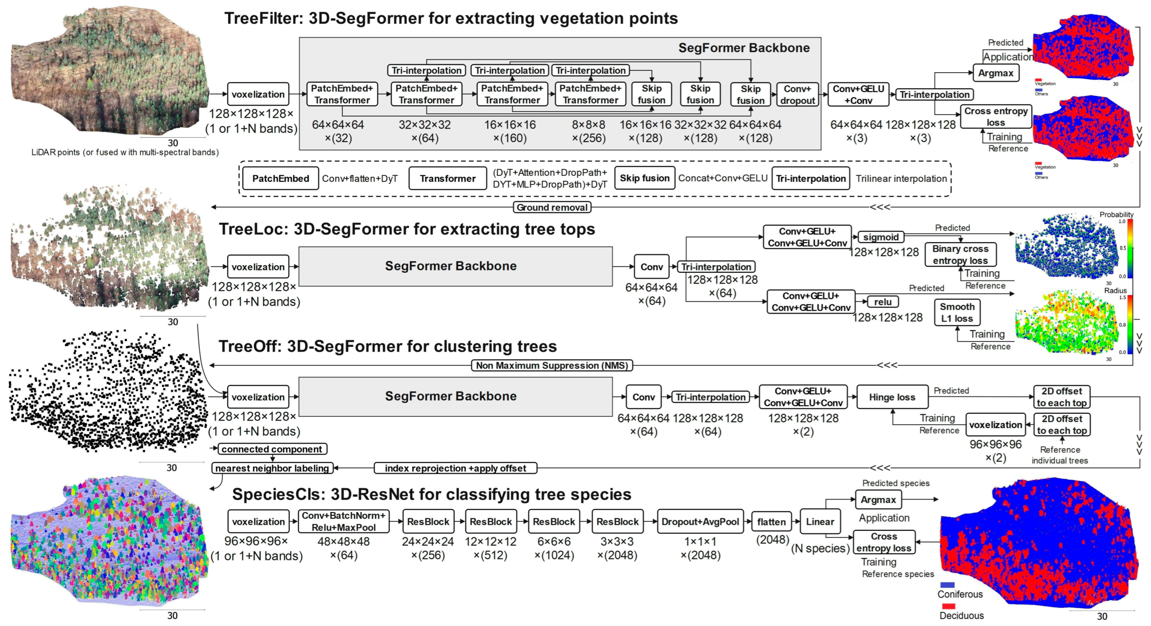
Figure 1. Reclaimed wellsite locations used for collecting RS and ground vegetation data within Alberta’s portion of the North American boreal zone [33]. Tree cover percentage is based on land cover data derived from MODIS imagery [34].
Remotesensing 17 03440 g001
Figure 2. Workflow for individual-tree analysis from UAV-borne RS data using the TreeAIBox plugin. * The LiDAR dataset has been used as a reference to align the MS orthomosaic.
Remotesensing 17 03440 g002
Figure 3. DL models for individual-tree-based wellsite LiDAR scan processing.
Remotesensing 17 03440 g003
Figure 4. Stepwise and spectral-wise model accuracy. Note that the accuracy metric is mIoU for TreeFilter, TreeOff, and SpeciesCls, and F1-score for TreeLoc.
Remotesensing 17 03440 g004
Figure 5. Height-specific F1-score of tree detection.
Remotesensing 17 03440 g005
Figure 6. Accuracy assessment of individual-tree extraction from UAV-LiDAR against field measurements: (a) comparison of LiDAR-derived and ground-measured tree heights; and (b) detection rate (%) and relative RMSE (%) by height class (m), with coniferous (green) and deciduous (yellow) proportions.
Remotesensing 17 03440 g006
Figure 7. Distribution of the five tree-detection error types by (a) height class, (b) species, and (c) site.
Remotesensing 17 03440 g007
Figure 8. Representative individual-tree RGB point clouds for four species: white spruce (Sw), lodgepole pine (Pl), balsam poplar (Pb), and willow (Sx).
Remotesensing 17 03440 g008
Figure 9. Slope (°), canopy fraction (%), stem density (sph), tree height (m), crown area (m2) and species composition (%) across five sites and three seasons: summer (green), autumn (orange), and spring (blue). Species compositions include coniferous (yellow), deciduous (green), and shrub (red).
Remotesensing 17 03440 g009
Figure 10. Box-plot illustrating the data distribution of individual-tree height (a), and crown area (b) across three seasons by site. The central line represents the median; box edges show the 25th and 75th quartiles. Whiskers extend to values within 1.5 times the interquartile range and points beyond the whiskers indicate outliers.
Remotesensing 17 03440 g010
Figure 11. Seasonal variation in model performance: (a) accuracy of the three DL modules (TreeFilter, TreeLoc, and SpeciesCls) across seasons; (b) relative height error compared to ground-surveyed tree heights. The central line represents the median; box edges show the 25th and 75th quartiles. Whiskers extend to values within 1.5 times the interquartile range and points beyond the whiskers indicate outliers.
Remotesensing 17 03440 g011
Table 1. General characteristics of the reclaimed wellsites selected for this study. Sw = white spruce, Pl = lodgepole pine, Pb = balsam poplar, and Sx = willow, stdev = standard deviation and n = number of trees.
Wellsite IDSpeciesMean Top Tree Height (stdev), mYear of PlantingReference Trees Measured (n)
262Sw, Pb, Sx4.07 (1.98)2007Sw (25), Pb (15), Sx (28)
350Sw, Sx 4.34 (1.06)2006Sw (28), Sx (17)
442Pl, Sw, Sx 2.91 (1.68)2009Pl (27), Sw (3), Sx (18)
460Pl, Pb, Sx 3.82 (1.23)2009Pl (25), Pb (20), Sx (6)
624Pl, Pb, Sw, Sx 4.79 (2.49)2009Pl (9), Pb (19), Sx (17)
Table 2. DL model parameter settings and sample separation.
StepsModel Hyperparameters
Voxel Division, Resolution
#Training Sample,
siteID (Date)
#Testing Sample,
siteID (Date)
TreeFilter128 × 128 × 128,
15 × 15 × 15 cm3
10 scans, All (August/October 2023)5 scans, All (May 2024)
TreeLoc128 × 128 × 128,
20 × 20 × 20 cm3
19,030 trees, All (August/October 2023)10,175 trees, All (May 2024)
TreeOff128 × 128 × 128, 10 × 10 × 20 cm31000 trees, Wellsite #262 (August 2023)297 trees, Wellsite #262 (August 2023)
SpeciesCls96 × 96 × 96, 30 × 30 × 30 cm3172 trees, Matched trees from field sample74 trees, Matched trees from field sample
Table 3. Model accuracies with LiDAR point cloud data only, LiDAR + RGB data, and LiDAR + MS (red, red edge, green, NIR, and blue) data.
Module (Process)LiDAR Point Cloud Only *LiDAR + RGB *LiDAR + MS *
TreeFilter: Vegetation filteringmIoU = 0.93mIoU = 0.93mIoU = 0.93
TreeLoc: Tree top detectionPrecision = 0.87Precision = 0.89Precision = 0.89
Recall = 0.79Recall = 0.77Recall = 0.78
F1 = 0.83F1 = 0.83F1 = 0.83
TreeOff: Tree segmentationmIoU = 0.83mIoU = 0.83mIoU = 0.84
Species classificationmIoU = 0.78mIoU = 0.84mIoU = 0.88
* Training iterations for comparisons were capped at 80,000 iterations to ensure consistency.
Disclaimer/Publisher’s Note: The statements, opinions and data contained in all publications are solely those of the individual author(s) and contributor(s) and not of MDPI and/or the editor(s). MDPI and/or the editor(s) disclaim responsibility for any injury to people or property resulting from any ideas, methods, instructions or products referred to in the content.