Estimation of Forest Aboveground Biomass in China Based on GEDI and Sentinel-2 Data: Quantitative Analysis of Optical Remote Sensing Saturation Effect and Terrain Compensation Mechanisms

Highlights

What are the main findings?

• This study generated a high-resolution (200 m) forest aboveground biomass (AGB) map of China and provides a national-scale quantitative analysis of optical saturation thresholds. Single-band reflectance saturates at ~80 Mg·ha⁻¹, while certain spectral indices used in this study (NDSIs) delay saturation to 100–150 Mg·ha⁻¹.
• It systematically uncovers the compensatory role of topographic factors. Terrain features like slope and elevation variability stably support AGB prediction in medium-to-high biomass regions (<300 Mg·ha⁻¹), mitigating the impact of optical saturation.

What is the implication of the main finding?

• The proposed analytical framework offers a physically interpretable and transferable approach for quantifying saturation and compensation mechanisms, guiding integration of multi-source data (e.g., radar/SAR) to overcome optical saturation.
• This work clearly delineates the potential and limitations of optical imagery, providing methodological guidance for large-scale, long-term biomass monitoring and historical AGB reconstruction.

Abstract

Forests store substantial amounts of aboveground biomass (AGB) and play a critical role in the global carbon cycle. Optical remote sensing offers long-term, large-scale monitoring capabilities; however, spectral saturation in high-biomass regions limits the accuracy of AGB estimation. Although radar and LiDAR data can mitigate the saturation problem, optical imagery remains irreplaceable for continuous, multi-decadal monitoring from regional to global scales. Nevertheless, quantitative analyses of nationwide optical saturation thresholds and compensation mechanisms are still lacking. In this study, we integrated high-accuracy AGB estimates from the Global Ecosystem Dynamics Investigation (GEDI) L4A product, Sentinel-2 optical imagery, and topographic variables to develop a 200 m resolution Light Gradient Boosting Machine (LightGBM) machine learning model for forests in China. Stratified error analysis, locally weighted scatterplot smoothing (LOWESS) curves, and SHapley Additive exPlanations (SHAP) were employed to quantify optical saturation thresholds and the compensatory effects of topographic features. Results showed that estimation accuracy declined markedly when AGB exceeded approximately 300 Mg·ha⁻¹. Red and red-edge bands saturated at around 80 Mg·ha⁻¹, while certain spectral indices delayed the threshold to 100–150 Mg·ha⁻¹. Topographic features maintained stable contributions below 300 Mg·ha⁻¹, providing critical compensation for AGB prediction in high-biomass areas. This study delivers a high-resolution national AGB dataset and a transferable analytical framework for saturation mechanisms, offering methodological insights for large-scale, long-term optical AGB monitoring.

1. Introduction

Forest aboveground biomass (AGB), as the energy foundation and material source for forest ecosystem functioning, is a key indicator for evaluating forest health and carbon storage capacity [1]. Accurate monitoring of forest AGB is crucial for carbon accounting, forest ecosystem management, and understanding global climate change. While long-term and continuous monitoring of AGB is important for evaluating temporal dynamics and supporting carbon neutrality policies, current large-scale monitoring remains challenging due to the limitations of traditional methods.

Traditional AGB estimation methods often rely on field surveys and allometric equations [2]. While these approaches offer high accuracy, they are limited by sparse plot distribution, high data acquisition costs, and poor spatial representativeness, making them insufficient for supporting continuous monitoring at the national scale. Remote sensing, with its advantages of broad spatial coverage, high temporal resolution, and automation, has become the mainstream tool for forest AGB estimation.

Remote sensing-based AGB estimation commonly uses three types of data sources: microwave radar, LiDAR, and optical imagery [3]. Microwave Synthetic Aperture Radar (SAR) can penetrate clouds and portions of vegetation, and its backscattered signals reflect surface geometry, roughness, and dielectric properties, making it suitable for monitoring forest structure [4]. However, SAR data are complex to interpret, more susceptible to speckle noise, and often require sophisticated pre-processing, which limits their use in nationwide AGB estimation. LiDAR can penetrate forest canopies and provide detailed vertical structural information (e.g., canopy height and volume), allowing highly accurate AGB estimation [5]. However, airborne LiDAR data are expensive, while spaceborne LiDAR typically lacks full spatial coverage. Optical remote sensing, highly sensitive to vegetation density [6], offers low acquisition and processing costs, globally available datasets, and long-term consistency. These characteristics make optical imagery particularly suitable for constructing large-scale AGB datasets over extended time periods.

While Vegetation Optical Depth (VOD) derived from passive microwave sensors has been successfully used for national and global AGB estimation, its coarse spatial resolution (typically 0.25°) limits its applicability for medium-to-high-resolution studies [7,8,9]. In contrast, optical imagery provides decades-long continuous observations at medium-to-high spatial resolutions (10–30 m), making it the only feasible data source for constructing high-resolution, long-term AGB datasets across China and similar regions. While SAR data offer continuous monitoring capabilities, their historical record is much shorter, limiting their suitability for building multi-decadal AGB time series.

A major limitation of optical imagery is spectral saturation in high-biomass regions. Spectral saturation occurs when the reflectance signal becomes insensitive to increases in AGB beyond a certain threshold, particularly in dense or structurally complex forests [10]. Although some studies have attempted to mitigate saturation effects by integrating optical data with radar or LiDAR [11,12], optical data remain the foundational input for large-scale, long-term AGB estimation due to their accessibility and historical continuity.

In addition, topographic variables, including elevation, slope, and aspect, have been shown to influence vegetation growth and optical reflectance patterns, affecting AGB estimation accuracy [13,14].

Therefore, under the constraint of relying primarily on optical data, it becomes essential to understand the saturation behavior and model errors in high AGB regions, in order to enhance the reliability and applicability of optical AGB estimation. Existing studies in China have mainly focused on regional scales. For instance, Sa et al. quantified saturation levels of combined variables in Saihanba Forest, Hebei Province, analyzing the limitations of AGB estimation saturation [15]. Wu et al. examined optical saturation in 20 regions across Yunnan, exploring the individual, interaction, and combined effects of climate, soil, and topography on saturation [16]. Another study by Wu et al. estimated saturation levels in a county of Heilongjiang Province [17], while Zhao et al. used a spherical model to quantify AGB saturation for different vegetation types in parts of Zhejiang Province [18]. These studies, however, rely on small-scale field data, limiting their ability to generalize findings nationwide. This limits the assessment of national-level saturation thresholds in high-AGB regions across China.

Machine learning has become a widely adopted approach for forest AGB estimation [3]. In remote sensing-based modeling, field measurements are critical for linking signals to actual biomass, but such measurements are time-consuming and labor-intensive [3,19], which limits their applicability for large-scale AGB estimation and monitoring.

The release of the Global Ecosystem Dynamics Investigation (GEDI) mission has provided a breakthrough. Its Level 4A (L4A) product serves as a high-accuracy reference for global AGB modeling. By using GEDI-derived estimates to complement traditional field measurements, large-scale inversion and monitoring of AGB can be achieved [20,21]. Recently, Cai et al. used GEDI L4A as a reference for mapping forest AGB across China from 1985 to 2023, leveraging long-term optical imagery for national-scale time-series estimation [22]. While this study achieved large-scale inversion, it focused on mapping accuracy and temporal modeling, without detailed investigation of spectral saturation mechanisms and error structures in high-biomass regions.

Addressing this research gap, the present study employs GEDI L4A AGB estimates as modeling labels, combined with Sentinel-2 multispectral imagery and topographic variables, to construct a 200 m resolution forest AGB estimation model at the national scale. Sentinel-2 was selected due to its high spatial resolution (10–20 m), frequent revisit, and rich spectral bands, making it particularly suitable not only for national-scale AGB estimation but also for analyzing error structures and optical saturation mechanisms. This also provides a methodological basis for future studies integrating Landsat historical imagery or other optical datasets for long-term AGB mapping and mechanism analysis.

This study focuses on understanding prediction error mechanisms caused by spectral saturation in high-biomass areas. Unlike previous studies that primarily targeted mapping accuracy, this work presents a national-scale analysis of spectral saturation mechanisms using optical inputs, along with the compensatory role of topography.

The specific innovations of this study include the following:

• Quantifying optical saturation thresholds at the national scale, defining the performance boundaries of different spectral bands and indices in medium-to-high AGB regions;
• Systematically evaluating the compensatory role of topographic variables in high AGB areas, revealing how they maintain prediction accuracy under spectral information deficiency;
• Proposing a transferable mechanism analysis framework that quantitatively reveals changes in feature contributions through grouped error analysis, LOWESS response curves, and SHAP model interpretation, extendable to other countries or global scales;
• Producing a nationwide 200 m resolution AGB data product and conducting regional validation using forest volume data, providing support for ecological monitoring and carbon stock estimation.

2. Materials and Methods

2.1. Study Area Overview

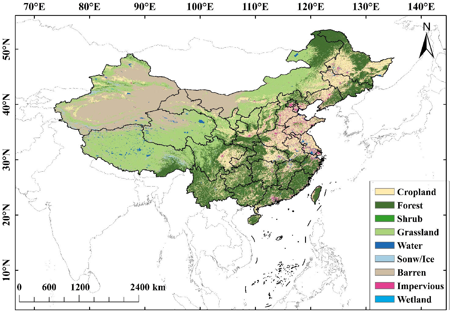
China is located in East Asia, on the western edge of the Pacific Ocean, covering a land area of approximately 9.6 million square kilometers—ranking as the third-largest country in the world after Russia and Canada. According to the 2023 China Statistical Yearbook, the national forest area reached 220.45 million hectares in 2022, including 80.03 million hectares of planted forests, with a forest coverage rate of 22.96% [23]. Forests are mainly distributed in the northeastern, southwestern, and southeastern regions, encompassing not only vast plains but also numerous remote and inaccessible areas such as high mountains, deep valleys, and dense woodlands. The region’s vast and complex terrain highlights the importance of large-scale, non-contact monitoring methods for forest resources. The study area is shown in Figure 1.

2.2. Methodology

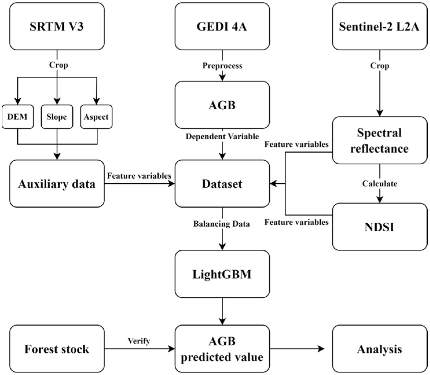
This study uses forest aboveground biomass (AGB) from the GEDI Level 4A product as the dependent variable. The independent variables include topographic variables—digital elevation model (DEM), slope, and aspect—derived from the SRTM Version 3 dataset, as well as multispectral reflectance and normalized difference spectral indices (NDSI) calculated from Sentinel-2 Level 2A imagery (band combinations for all NDSIs are listed in

Table A1. NDSI band combinations used in this study.

NDSI Name	Band Combination	NDSI Name	Band Combination	NDSI Name	Band Combination
NDSI_B2_B3	(B2, B3)	NDSI_B2_B4	(B2, B4)	NDSI_B2_B5	(B2, B5)
NDSI_B2_B6	(B2, B6)	NDSI_B2_B7	(B2, B7)	NDSI_B2_B8	(B2, B8)
NDSI_B2_B8A	(B2, B8A)	NDSI_B2_B11	(B2, B11)	NDSI_B2_B12	(B2, B12)
NDSI_B3_B4	(B3, B4)	NDSI_B3_B5	(B3, B5)	NDSI_B3_B6	(B3, B6)
NDSI_B3_B7	(B3, B7)	NDSI_B3_B8	(B3, B8)	NDSI_B3_B8A	(B3, B8A)
NDSI_B3_B11	(B3, B11)	NDSI_B3_B12	(B3, B12)	NDSI_B4_B5	(B4, B5)
NDSI_B4_B6	(B4, B6)	NDSI_B4_B7	(B4, B7)	NDSI_B4_B8	(B4, B8)
NDSI_B4_B8A	(B4, B8A)	NDSI_B4_B11	(B4, B11)	NDSI_B4_B12	(B4, B12)
NDSI_B5_B6	(B5, B6)	NDSI_B5_B7	(B5, B7)	NDSI_B5_B8	(B5, B8)
NDSI_B5_B8A	(B5, B8A)	NDSI_B5_B11	(B5, B11)	NDSI_B5_B12	(B5, B12)
NDSI_B6_B7	(B6, B7)	NDSI_B6_B8	(B6, B8)	NDSI_B6_B8A	(B6, B8A)
NDSI_B6_B11	(B6, B11)	NDSI_B6_B12	(B6, B12)	NDSI_B7_B8	(B7, B8)
NDSI_B7_B8A	(B7, B8A)	NDSI_B7_B11	(B7, B11)	NDSI_B7_B12	(B7, B12)
NDSI_B8_B8A	(B8, B8A)	NDSI_B8_B11	(B8, B11)	NDSI_B8_B12	(B8, B12)
NDSI_B8A_B11	(B8A, B11)	NDSI_B8A_B12	(B8A, B12)	NDSI_B11_B12	(B11, B12)

). In this study, the forest extent was delineated using the China Land Cover Dataset (CLCD), and only pixels classified as forest were included for AGB modeling and analysis.

The Light Gradient Boosting Machine (LightGBM) algorithm is applied to build a predictive model to estimate AGB at the national scale. Model performance is assessed using standard metrics, including the coefficient of determination (R²) and root mean square error (RMSE). A spectral saturation mechanism analysis is then conducted on the prediction results. The accuracy of the predicted AGB is indirectly validated using forest stock volume data from the China Statistical Yearbook.

This method is reproducible in other countries by simply substituting land cover, optical imagery, and terrain data, while keeping the modeling workflow consistent. The technical workflow of this study is illustrated in Figure 2.

2.3. Data and Preprocessing

This study utilizes multi-source remote sensing data, including optical imagery, LiDAR products, terrain data, and land cover datasets, to construct a high-accuracy forest aboveground biomass (AGB) inversion model. Administrative boundaries for image clipping are obtained from GeoJSON files provided by Tianditu [24].

The datasets used for AGB inversion are summarized in

Table 1. Overview of datasets used for forest aboveground biomass (AGB) inversion in this study.

Data	Resolution	Time	Purpose	Platform
CLCD	30 m	2022	Forest Mask	Zenodo [25]
Sentinel-2 L2A	10–20 m	2022	Spectral feature	GEE
GEDI 4A	~25 m	2022	AGB ground truth	EARTHDATA
SRTM V3	30 m	2000	Terrain feature	GEE

.

2.3.1. CLCD Dataset

The CLCD (Chinese Land Cover Dataset) is a 30 m resolution land cover product developed by the team led by Jie Yang and Xin Huang, spanning from 1985 to 2023. It is generated using Landsat satellite imagery via the Google Earth Engine platform. The dataset covers nine land cover classes: Cropland, Forest, Shrub, Grassland, Water, Snow/Ice, Barren, Impervious, and Wetland. Training samples for the random forest classification were constructed based on visual interpretation of Landsat imagery. The overall classification accuracy, calculated based on 5463 visually interpreted samples, reaches 79.31%. The classification workflow combines random forest modeling, spatio-temporal filtering, and logical post-processing. Furthermore, validation using 5131 independent third-party samples indicates that CLCD achieves higher overall accuracy compared to MCD12Q1, ESACCI_LC, FROM_GLC, and GlobeLand30 products. Compared to other thematic products, CLCD shows strong consistency in time-series data related to forest vegetation changes, water bodies, and impervious surfaces [25]. One key advantage of the CLCD is its provision of annually updated land cover maps. In this study, the CLCD is used to extract forest pixels across China as the primary analysis targets.

2.3.2. Sentinel-2 L2A

This study utilized surface reflectance data from Sentinel-2 Level-2A (L2A), sourced from the Harmonized Sentinel-2 MSI: MultiSpectral Instrument, Level-2A dataset available on the Google Earth Engine (GEE) platform. This dataset is derived from Level-1C top-of-atmosphere (TOA) products through the Sen2Cor atmospheric correction process [26]. To capture forest conditions during the growing season, we generated a cloud-free median composite using all available images from 2022. Forest regions were extracted, and all image preprocessing steps—including cloud masking, band resampling, and median compositing—were conducted within GEE. Pixels with a cloud probability greater than 20% (based on the Sentinel-2 cloud probability dataset) were removed. Bands B2, B3, B4, and B8 (10 m resolution) were resampled to 20 m using bilinear interpolation to match the resolution of lower-resolution bands. The ten spectral bands used are listed in

Table 2. Selected band information of the Sentinel-2 satellite.

Band	Band Name	Center Wavelength	Spatial Resolution
B2	B	492	10
B3	G	559	10
B4	R	665	10
B5	RE1	704	20
B6	RE2	740	20
B7	RE3	781	20
B8	NIR1	833	10
B8A	NIR2	864	20
B11	SWIR1	1612	20
B12	SWIR2	2194	20

.

2.3.3. GEDI 4A

The Global Ecosystem Dynamics Investigation (GEDI) is a mission initiated by the National Aeronautics and Space Administration (NASA) that employs LiDAR technology to measure and monitor Earth’s ecosystems. Successfully launched on 5 December 2018, GEDI aims to acquire high-resolution data on the three-dimensional structure and AGB distribution of global forests, thereby supporting ecological monitoring and management efforts. GEDI produces footprints approximately 25 m in diameter, with a spacing of 60 m along-track and about 600 m between adjacent ground tracks. The key parameters of the GEDI system are summarized in

Table 3. Gedi parameter information.

Parameter	Size
Wavelength	1064 nm
Footprint Size	25 m
Geolocation Error	8 m
Along-track Distance	60 m
Cross-track Distance	600 m

[27].

The GEDI Level 4A (L4A) product (version 2) used in this study was obtained from the Oak Ridge National Laboratory Distributed Active Archive Center (ORNL DAAC) [27]. Previous studies have demonstrated that GEDI products can serve as reliable ground-truth data sources for forest AGB estimation within a certain accuracy range [20,22,28,29,30]. In this study, L4A data, which provide footprint-level estimates of AGB and associated prediction uncertainties, were used as reference values for model prediction. The GEDI data used in this study cover the entire year of 2022. The retained fields from L4A are listed in

Table 4. Gedi read field information.

Field Name	Unit	Description
agbd	Mg·ha−1	Predicted aboveground biomass density
agbd_se	Mg·ha−1	Standard error of aboveground biomass
degrade_flag		Flag indicating degradation and/or decline
l4_quality_flag		Flag simplifying selection of most useful biomass predictions
lat_lowestmode	°	Latitude of the lowest mode center
lon_lowestmode	°	Longitude of the lowest mode center

.

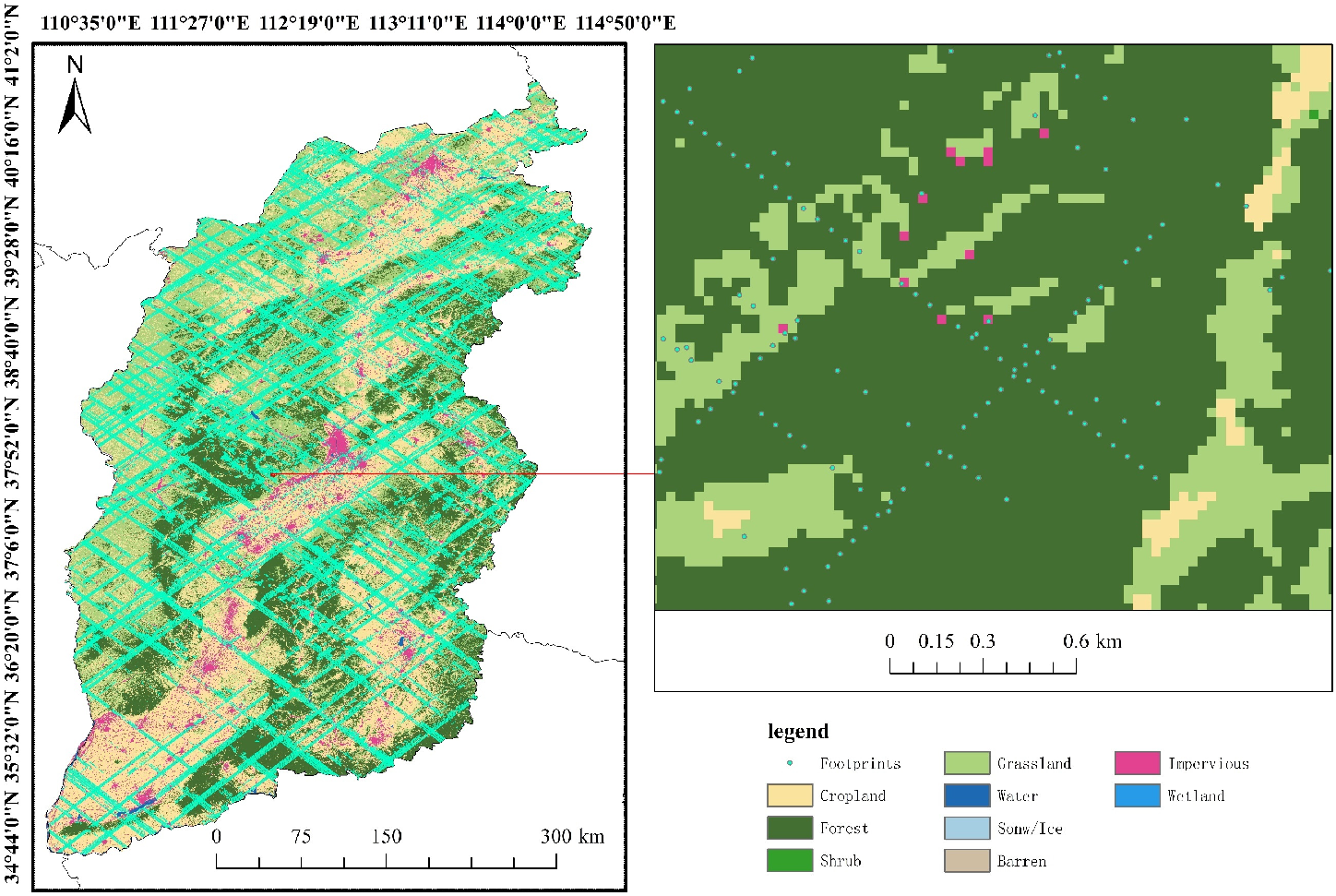
Spatial coordinates of each GEDI footprint were obtained from ‘lat_lowestmode’ and ‘lon_lowestmode’. Quality filtering was conducted using relevant quality flags. Only GEDI measurements with a relative standard error of less than 50% and a slope less than 30° (calculated from the DEM) were retained [31]. The spatial distribution of filtered GEDI footprints (taking Shaanxi Province as an example) is shown in Figure 3. Forest land cover data used for filtering were obtained from the CLCD dataset.

Finally, footprint points located within forest areas were selected based on the CLCD land cover dataset, corresponding to the dark green regions shown in the figure.

2.3.4. SRTM

This study utilized the NASA SRTM Digital Elevation Model (DEM) 30 m dataset available on the Google Earth Engine (GEE) platform to obtain topographic variables within the study area. Based on research requirements, the elevation band was selected, and to match the spatial resolution of Sentinel-2 imagery, the DEM was resampled to 20 m resolution using bilinear interpolation. After calculating slope and aspect from the digital elevation model (DEM), the three topographic variables—DEM (elevation), slope, and aspect—were extracted specifically within forested areas identified by the CLCD dataset.

2.4. Feature Extraction and Grid Aggregation

2.4.1. Optical Feature Extraction

In addition to the 10 original Sentinel-2 spectral bands listed in Table 2 used as spectral input features for the model, this study further constructed normalized difference spectral indices (NDSIs) derived from all possible combinations of any two bands. The calculation formula for NDSI is given in Equation (1), where $B_{\mathrm{i}}$ and $B_{\mathrm{j}}$ represent the band numbers. Previous studies have shown that NDSIs facilitate vegetation type discrimination [32] and can be used for forest biomass inversion [33]. Compared to single-band reflectance, NDSIs exhibit higher stability in overcoming external interference factors such as atmospheric conditions, illumination, and terrain.

$$NDSI={\displaystyle \frac{\left(B_{\mathrm{i}}-B_{\mathrm{j}}\right)}{\left(B\mathrm{i}+B_{\mathrm{j}}\right)}},$$

(1)

In addressing the saturation issue, this study utilized all 45 possible NDSI combinations without prior feature selection, thereby avoiding the risk of missing optimal band combinations by relying solely on a limited set of predefined indices (e.g., NDVI). This approach provided richer spectral response information for subsequent error structure analysis, enabled data-driven identification of key spectral indices through model interpretation, and ensured reproducibility by eliminating subjective pre-modeling index screening. In our residual group analysis, NDSI–AGB fitting curves (LOWESS), and SHAP-based model interpretation, NDSI contributed to revealing model performance differences across AGB levels, particularly the saturation trends in medium- to high-biomass regions. Compared with traditional fixed vegetation indices (e.g., NDVI, EVI), NDSI offers more flexible combinations covering visible, near-infrared, and shortwave infrared bands, thereby enhancing the model’s responsiveness to differences in forest types and structures. The inclusion of NDSI not only enriched the spectral feature dimension of the model but also provided a comprehensive feature pool for subsequent mechanistic error analysis and model interpretability studies.

2.4.2. Topographic Variable Extraction

Slope and aspect were derived from the SRTM DEM using the ee.Terrain module within the Google Earth Engine (GEE) platform. All terrain layers, including DEM, slope, and aspect, were resampled to 20 m resolution using bilinear interpolation and masked to forested areas based on the CLCD dataset.

2.4.3. Grid Aggregation

To mitigate the geolocation uncertainty of GEDI footprints (approximately ±10 m) [34], we aggregated them into 200 m × 200 m grid cells. This approach, following Shendryk [20], effectively reduces random geolocation errors by averaging multiple footprints per cell. We retained only grid cells containing more than 7 high-quality GEDI footprints to ensure reliable AGB label calculation while maintaining a sufficient sample size.

For each retained grid cell, the forest AGB label was computed as the mean agbd value of all contained footprints. Correspondingly, the mean and standard deviation of Sentinel-2 band reflectance and topographic variables were calculated using only forest pixels (as classified by the CLCD dataset). The 45 Normalized Difference Spectral Indices (NDSIs) were then derived from these averaged band reflectances. Finally, the AGB label for each grid was matched with its computed spectral and topographic features for model training.

2.5. Aboveground Biomass Density Prediction Model Construction

This study systematically compared three mainstream machine learning algorithms: LightGBM, Random Forest (RF), and Support Vector Machine (SVM). A preliminary experiment was conducted using 10% of the final sample dataset. Since LightGBM and RF are both decision tree–based models, no data normalization was required, whereas data normalization was applied prior to training the SVM model. The results of the preliminary experiment are shown in

Table 5. Model preliminary experiment results table.

Algorithm	R2	RMSE	Time
LightGBM	0.61	38.53 Mg·ha−1	43.23 s
RF	0.61	38.79 Mg·ha−1	175.74 s
SVM	0.49	51.64 Mg·ha−1	442.53 s

. Note that this preliminary experiment used only 10% of the samples without hyperparameter tuning. After stratified sampling and hyperparameter optimization, the performance of the final model was significantly improved.

As shown in Table 5, LightGBM and RF models achieved the highest accuracy. Considering the large data volume for nationwide modeling (>37,000 samples), this study selected LightGBM as the AGB estimation model due to its shorter training time, which improves computational feasibility while maintaining accuracy.

2.5.1. LightGBM

LightGBM is an efficient gradient boosting decision trees (GBDT) implementation, optimized for large-scale, high-dimensional data [35]. Its core optimizations include a histogram-based algorithm for rapid splitting point identification, a leaf-wise growth strategy with depth limitation for enhanced accuracy, and techniques like Gradient-based One-Side Sampling (GOSS) and Exclusive Feature Bundling (EFB) to improve computational efficiency and handle sparse data [35].

These characteristics make LightGBM particularly suitable for the present study, which involves large-scale remote sensing data modeling tasks [36]. The algorithm demonstrates high computational efficiency and robust feature handling capabilities, which are essential for processing the high-dimensional input feature set (including spectral bands, topographic variables, and 45 NDSIs) and the substantial sample size at the national scale.

Compared to deep learning and other machine learning methods, LightGBM offers specific advantages for this research: (1) high computational efficiency suitable for large-scale, high-dimensional feature data; (2) inherent support for feature importance evaluation and model interpretability analysis, crucial for employing SHAP to investigate optical saturation mechanisms and topographic compensation effects; (3) demonstrated robustness and generalization capability under imbalanced sample distributions [37]. Consequently, LightGBM was selected for nationwide AGB inversion. This choice balances estimation accuracy with computational feasibility and supports subsequent mechanistic analysis.

2.5.2. Model Training

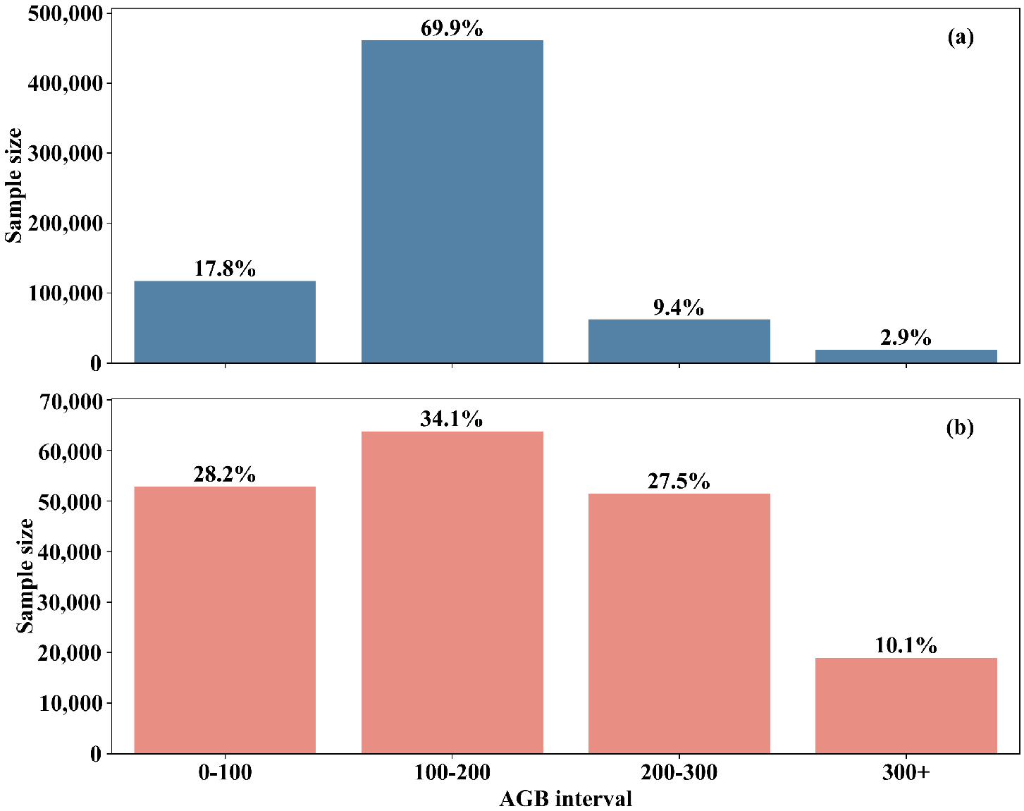
To alleviate the severe imbalance in the distribution of AGB samples, this study employed a value-based stratified downsampling strategy when constructing the training dataset. Specifically, the GEDI AGB samples were evenly divided into 30 bins according to their numerical range. The first 9 bins (low AGB with high frequency) were randomly downsampled so that the total number of samples in these bins matched the total number of samples in the remaining 21 bins (medium to high AGB). The balanced data distribution is shown in Figure 4.

This method effectively prevents overfitting to low AGB samples during model training while enhancing the model’s learning capability in medium to high biomass regions. The final balanced training dataset covers the full AGB range and exhibits good numerical uniformity and representativeness.

The balanced dataset uses AGB as the dependent variable, with features comprising the mean and standard deviation of 10 spectral bands and topographic variables, as well as the mean values of 45 NDSIs. Eighty percent of the data were used for training, and 20% were reserved as an independent test set. Within the training subset, hyperparameter optimization was performed using 5-fold cross-validation. In each fold, 80% of the training data were used for model fitting and 20% for validation. A grid search was conducted over key parameters (e.g., learning rate: 0.01–0.2, max depth: 2–15, number of leaves: 4–125) to determine the optimal hyperparameters. A quantile loss function (alpha = 0.5) was employed to mitigate the influence of high-AGB outliers during training. The optimal hyperparameter settings are listed in

Table 6. Hyperparameter information.

Hyperparameter	Optimal Value
metric	quantile
boosting_type	gbdt
objective	regression
learning_rate	0.1
num_leaves	58
min_child_samples	514
max_depth	2
alpha	0.5

.

2.5.3. Model Evaluation Metrics

To comprehensively assess the predictive performance of the developed models, this study selected the coefficient of determination (R²) and root mean square error (RMSE) as the primary evaluation metrics. R² measures the proportion of variance in the observed data explained by the model; values closer to 1 indicate a better fit. RMSE represents the average deviation between predicted and observed values; lower RMSE indicates higher prediction accuracy.

The formula for R² is given as follows:

$$R^2=1-{\displaystyle \frac{{\sum }_{i=1}^n{(y_i-{\widehat{y}}_i)}^2}{{\sum }_{i=1}^n{(y_i-\overline{y})}^2}}$$

(2)

where $y_i$ is the $i^{\mathrm{t}\mathrm{h}}$ observed value, ${\widehat{y}}_i$ is the model-predicted value, $\overline{y}$ is the mean of the observed values, and $n$ is the sample size.

The formula for RMSE is given as follows:

$$RMSE=\sqrt{{\displaystyle \frac{1}{n}}{\sum }_{i=1}^n{(y_i-{\widehat{y}}_i)}^2}$$

(3)

We report the R² and RMSE on the independent test set to ensure a robust evaluation.

2.5.4. Uncertainty Estimation

To assess the reliability of model predictions, the uncertainty of AGB estimates was quantified using a LightGBM-based quantile regression approach. Two models were trained with quantile parameters α = 0.025 and α = 0.975 to obtain the 2.5th and 97.5th percentiles of predicted AGB. The difference between these quantile predictions was used to calculate a 95% prediction interval, providing a robust measure of prediction uncertainty. This method is commonly used in machine learning [38,39] and has been successfully applied to estimate uncertainty in forest AGB prediction using LightGBM [20].

2.6. Saturation Mechanism Analysis Methods

2.6.1. Stratified Residual Analysis

To systematically evaluate the model’s predictive performance across different biomass levels and investigate potential saturation effects of optical features in high-biomass regions, this study employed a grouped residual analysis approach. Specifically, all samples in the test set were grouped according to the GEDI-provided AGB reference values (agbd_avg) with intervals of 100 Mg·ha⁻¹, divided into five categories: 0–100, 100–200, 200–300, 300–400, and >400 Mg·ha⁻¹. This interval was selected to ensure a statistically robust sample size in each stratum while being sufficiently precise to capture critical performance transitions.

For each group, key performance metrics including RMSE and mean bias (defined as the mean of predicted minus observed values) were calculated. These metrics quantify the model’s fit, error magnitude, and systematic bias trends within each AGB interval. Particularly, a sharp increase in RMSE accompanied by a negative shift in bias in high AGB bins is interpreted as a quantitative indication of optical feature saturation.

This analysis helps identify biomass levels at which the model performance deteriorates significantly, reflecting the applicability limits of optical remote sensing in dense forest areas, and provides a basis for subsequent error interpretation and mechanism investigation.

2.6.2. LOWESS Fitting Analysis

This study further explored the response characteristics of key spectral indices (NDSIs) across different biomass intervals. For the top two most important features selected from spectral reflectance, NDSI, and topographic variables, scatter plots against AGB were generated, followed by LOWESS curve fitting to examine whether response weakening, non-monotonicity, or failure occurred in high AGB ranges. This qualitative assessment aids in identifying the suitability of different band combinations for dense forest regions and supports optical saturation mechanism analysis.

2.6.3. SHAP Value Explanation Method

Model interpretability is a crucial factor influencing the scientific reliability of machine learning-based AGB inversion. To gain deeper insights into the model’s dependence on input features and their roles at varying biomass levels, this study employed SHAP (SHapley Additive exPlanations) to interpret the trained LightGBM model.

SHAP is a novel model explanation method based on game theory’s Shapley values, combining optimal credit allocation with local interpretability. It assigns an attribution value to each feature, representing its contribution to the model prediction, and is applicable to various machine learning models [40,41]. Without compromising model performance, SHAP can interpret tree-based or black-box models, making it suitable for evaluating feature importance rankings, response directions, and behavior under varying input values.

In this study, SHAP values were computed based on test set samples, and feature contribution distributions were visualized. By analyzing the distribution of SHAP values across feature value intervals, nonlinear feature responses or contribution inflection points can be revealed.

2.6.4. Spatial Residual Heatmaps

To further investigate the spatial distribution characteristics of model errors and possible systematic biases, spatial residual analysis was conducted. Residuals for each sample point were calculated as the difference between predicted and observed GEDI AGB values (Residual = Prediction − agbd_avg) to represent local prediction bias.

Spatial visualization included province-level average residual heatmaps, aggregating residuals by averaging within each province to analyze regional error distribution trends. Spatial residual analysis helps identify systematic errors associated with specific ecological zones, forest types, or terrain conditions, supporting understanding of model generalization and providing spatial guidance for future improvements.

2.7. Accuracy Validation Method

Stand volume refers to the total amount of timber and other biomass stored within a specific forested area, typically expressed in cubic meters (m³). The estimation of AGB often relies on stand volume and biomass conversion factors. According to the following formula, stand volume can be converted into AGB:

$$AGB=SV\times BEF$$

(4)

AGB refers to the aboveground biomass of forests; $SV$ denotes the stand volume; $BEF$ is the Biomass Expansion Factor, an empirical coefficient based on different tree species and growth conditions, commonly used to convert volume into biomass.

To validate whether the model-predicted AGB can reliably represent the aboveground biomass density across China, the predicted forest AGB was multiplied by the pixel area to obtain the total predicted AGB per pixel. Subsequently, the total forest AGB was aggregated by province and compared with the 2022 provincial stand volume data from the 2023 China Statistical Yearbook. Spearman’s rank correlation coefficient was employed as the evaluation metric for consistency analysis. Even without applying precise BEF values, the relative ranking of total predicted AGB across provinces should correspond closely to that of total stand volume, which can serve to indirectly validate the model’s macro-scale accuracy.

3. Results

3.1. Overall Model Performance Evaluation

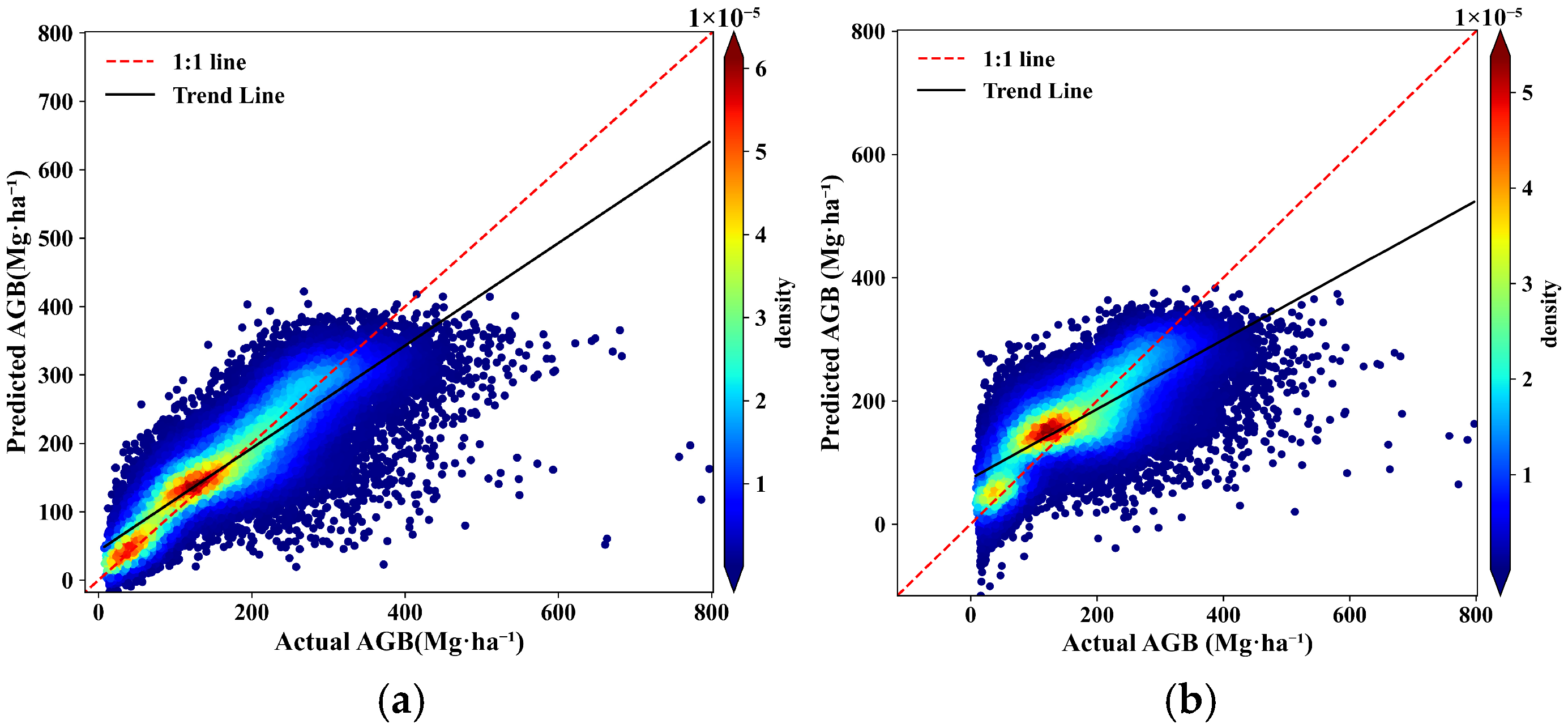
The model achieved R² values of 0.78 and 0.76 on the training and testing datasets, respectively, with comparable RMSE values. The RMSE on the testing set was 47.73 Mg·ha⁻¹, indicating good generalization ability without obvious overfitting. The scatter density plot of predictions versus observations on the test set is shown in Figure 5a. Although the overall accuracy is satisfactory, relatively larger errors exist in high AGB ranges, warranting further stratified analysis. To further provide a more intuitive comparison of the contribution of topographic factors, we additionally developed a model excluding topographic variables and generated the corresponding scatter density plot (Figure 5b) for direct comparison with the original model including topography. The trend line in Figure 5b shows a noticeably lower slope, indicating the contribution of topographic variables to improving model accuracy and mitigating saturation effects.

3.2. Stratified Error Analysis by AGB

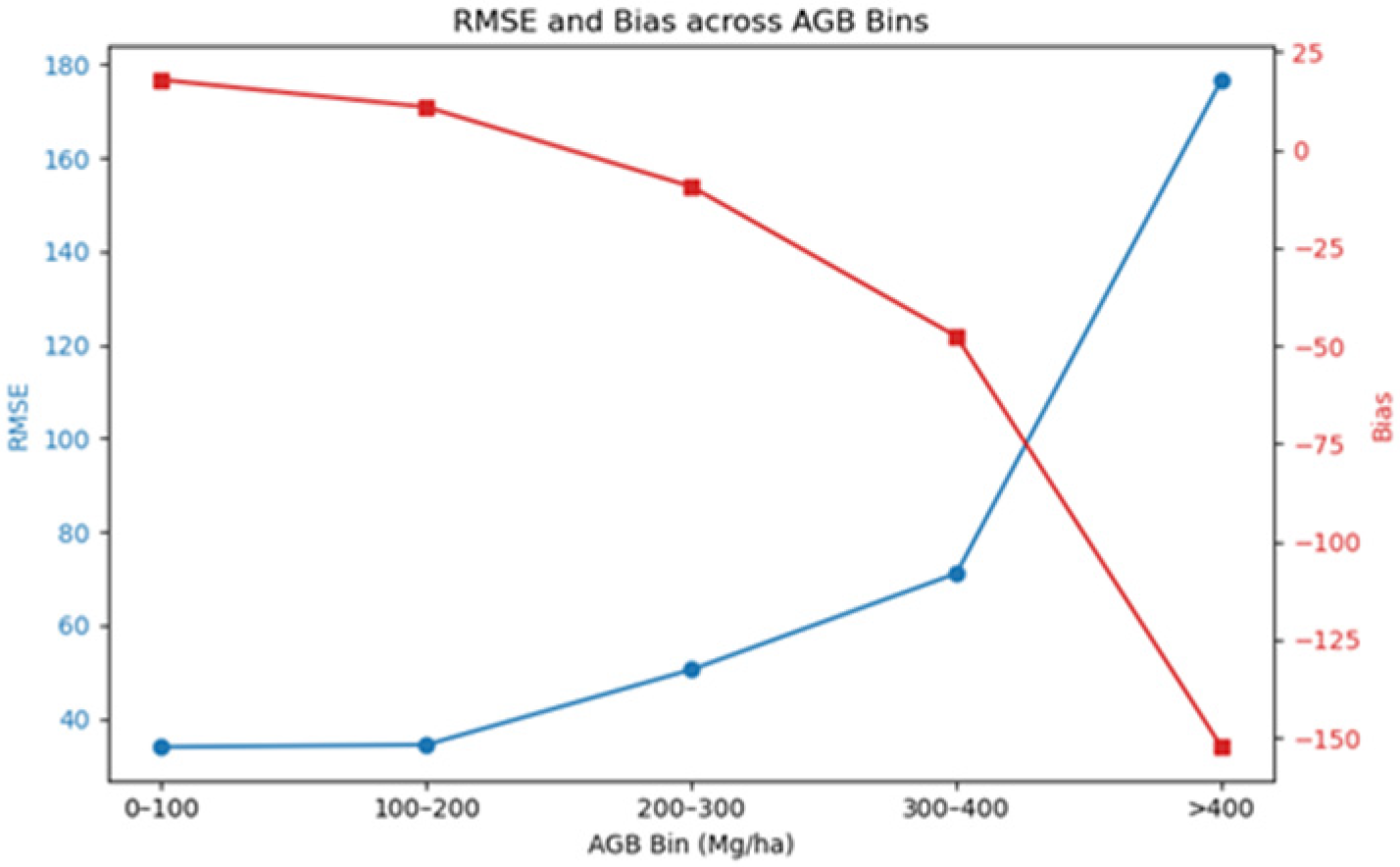
Following the stratified residual analysis method described in Section 2.6.1, the vali-dation dataset was divided into five AGB intervals and the corresponding RMSE and mean bias were computed. The stratified error metrics are summarized in

Table 7. AGB layered error table.

AGB (Mg·ha−1)	N	Percentage	RMSE	Bias
0–100	10,578	28.10%	33.95	17.90
100–200	12,767	33.92%	34.41	10.95
200–300	10,470	27.81%	50.49	−9.35
300–400	3353	8.91%	71.08	−47.58
>400	475	1.26%	176.74	−152.39

, and the RMSE and Bias trends are shown in Figure 6.

Both RMSE and Bias increase with AGB levels, especially in the >400 Mg·ha⁻¹ range, where RMSE reaches 176.74 Mg·ha⁻¹ and mean underestimation exceeds 152 Mg·ha⁻¹. This indicates systematic underestimation in extremely high biomass areas, likely associated with spectral saturation effects. However, due to the relatively sparse sample size in these high biomass regions, the overall impact on model performance is limited. Consequently, the model still maintains high accuracy at the national scale, though future work requires more independent validation data from high biomass areas to further confirm saturation severity and model bias in this range.

In this study, the model’s estimated AGB saturation threshold is approximately 300 Mg·ha⁻¹; beyond this value, predictions show significant bias and decreased reliability.

3.3. SHAP Interpretation

To better understand the contribution of different features to AGB prediction, SHAP values were calculated for the trained LightGBM model. Figure 7 shows the top 20 features ranked by their mean absolute SHAP values along with the distribution of their SHAP values. Spatial and topographic variables such as lon_lowestmode, dem_std, and slope_avg exhibited the highest importance in the model, while certain spectral variables (e.g., band_B4_avg, band_B5_avg, NDSI_B2_B4_avg) also demonstrated relatively high overall importance.

3.4. Spectral Saturation Curves

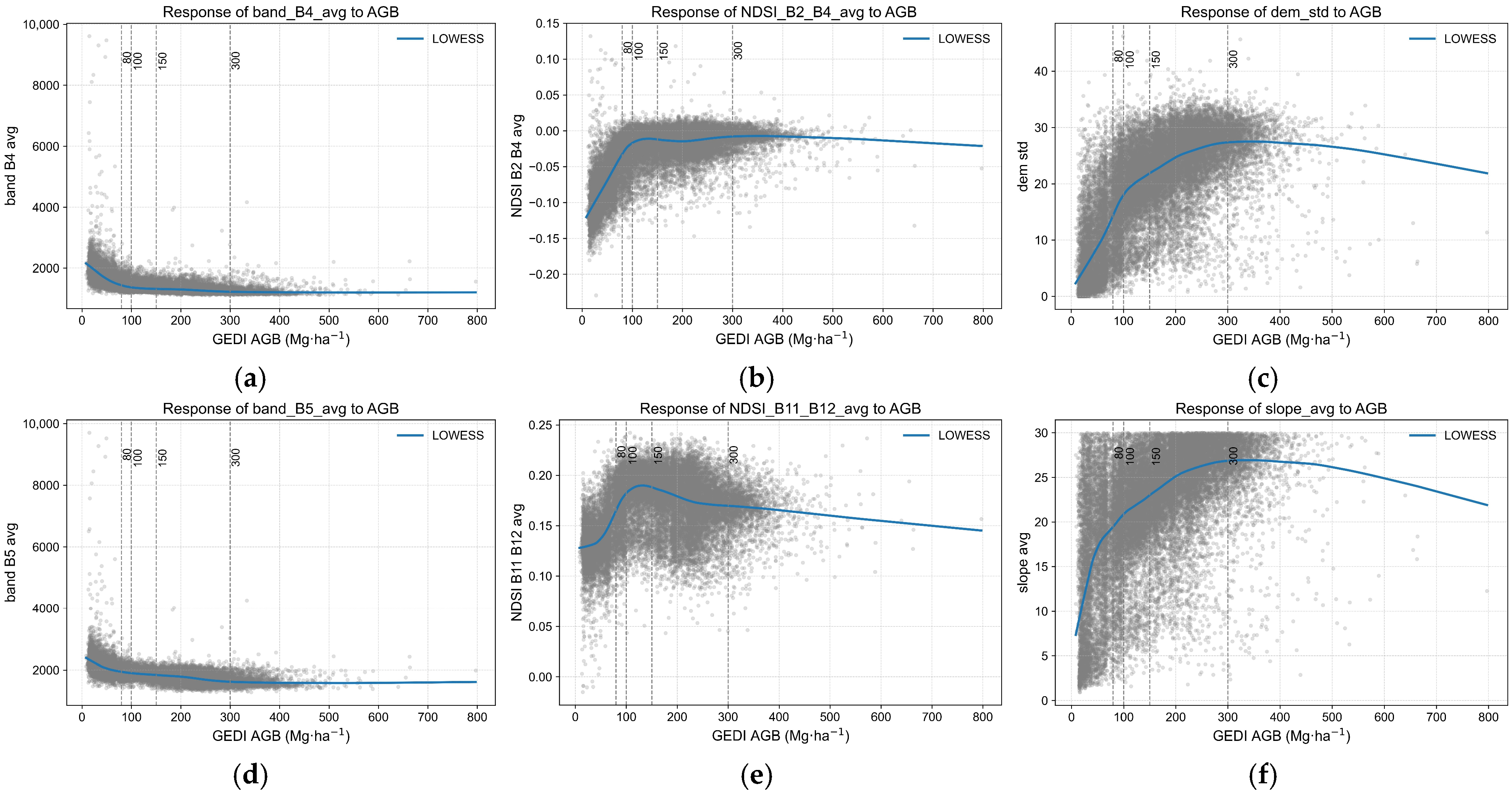
To further investigate the response relationship between spectral features and AGB, the top two original bands, NDSI indices, and topographic variables ranked by SHAP values were selected for LOWESS curve fitting to analyze their saturation trends. These features include “band_B4_avg,” “band_B5_avg,” “NDSI_B2_B4_avg,” “NDSI_B11_B12_avg,” “dem_std,” and “slope_avg.” The resulting curves for these features are shown in Figure 8.

The results show that the two band reflectance features (Figure 8a,d) exhibit a monotonically decreasing trend with increasing AGB, reaching a plateau around 80 Mg·ha⁻¹, reflecting a typical spectral saturation phenomenon. In contrast, the NDSI-type indices have higher saturation thresholds. The curve of NDSI_B2_B4_avg (Figure 8b) begins to plateau between 100–150 Mg·ha⁻¹, while NDSI_B11_B12_avg (Figure 8e) reaches a peak within the 100–150 Mg·ha⁻¹ range, then reverses slope and shows a stable negative trend from 150–200 Mg·ha⁻¹, gradually plateauing after 200–250 Mg·ha⁻¹ with a slight declining trend. This suggests that this index exerts a mild adverse effect on predictions in medium-to-high biomass areas.

Compared with spectral variables, the topographic features slope_avg (Figure 8f) and dem_std (Figure 8c) maintained a strong positive relationship with AGB when AGB < 300 Mg·ha⁻¹, but exhibited a slight declining trend when AGB > 300 Mg·ha⁻¹, indicating that they could not capture AGB variations beyond this threshold. This pattern is consistent with the observed decline in model prediction accuracy in high-biomass regions. These results suggest that topographic features play a significant supporting role in model prediction for medium- to high-biomass areas, serving as important complementary variables when spectral information becomes saturated. However, in extremely high-biomass regions (>300 Mg·ha⁻¹), their response trends weaken or even decline, implying that their contribution to prediction accuracy is also limited under conditions of highly homogeneous canopy structure.

3.5. Spatial Distribution of Residuals

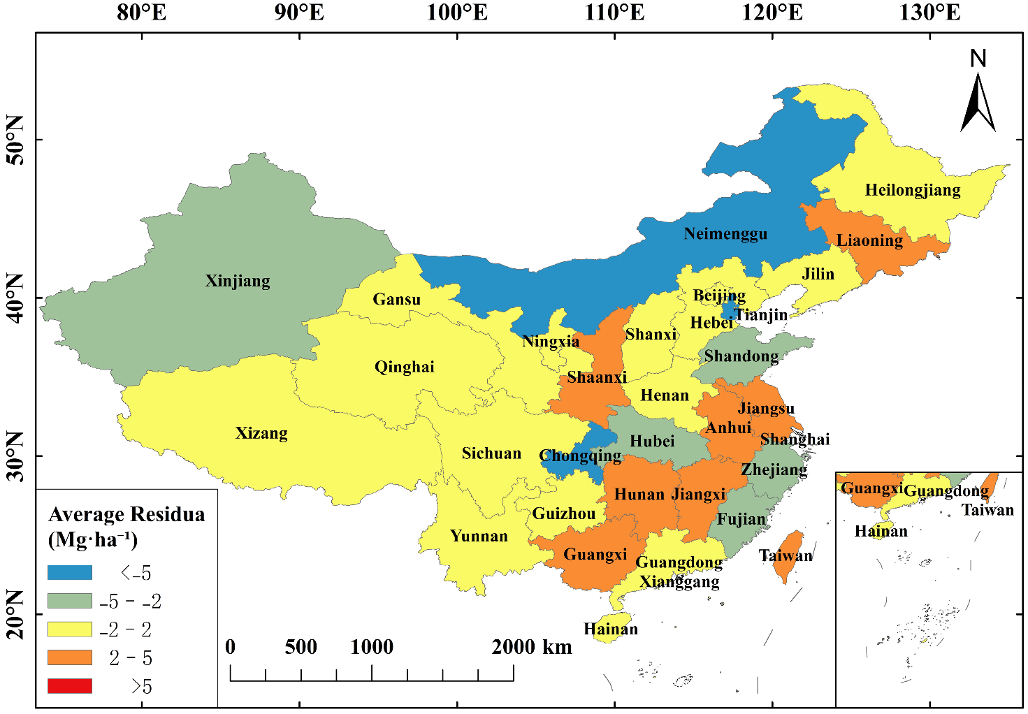
To identify the spatial patterns of model prediction errors, this study calculated the average residuals (Residual = Prediction − agbd_avg) for each provincial administrative region based on the test set samples. A province-level residual heatmap at the national scale was generated (Figure 9). The colors in the map indicate the magnitude and direction of the average residuals, where blue represents regions with overall underestimation and red indicates regions with overall overestimation.

The results indicate that the model demonstrates good spatial stability across most regions but still exhibits notable regional systematic biases. Specifically, systematic underestimation is observed in areas such as Chongqing, Tianjin, and Inner Mongolia, whereas slight overestimation occurs in eastern and southern provinces such as Jiangsu, Jiangxi, and Hunan.

3.6. Forest AGB Distribution Map in China

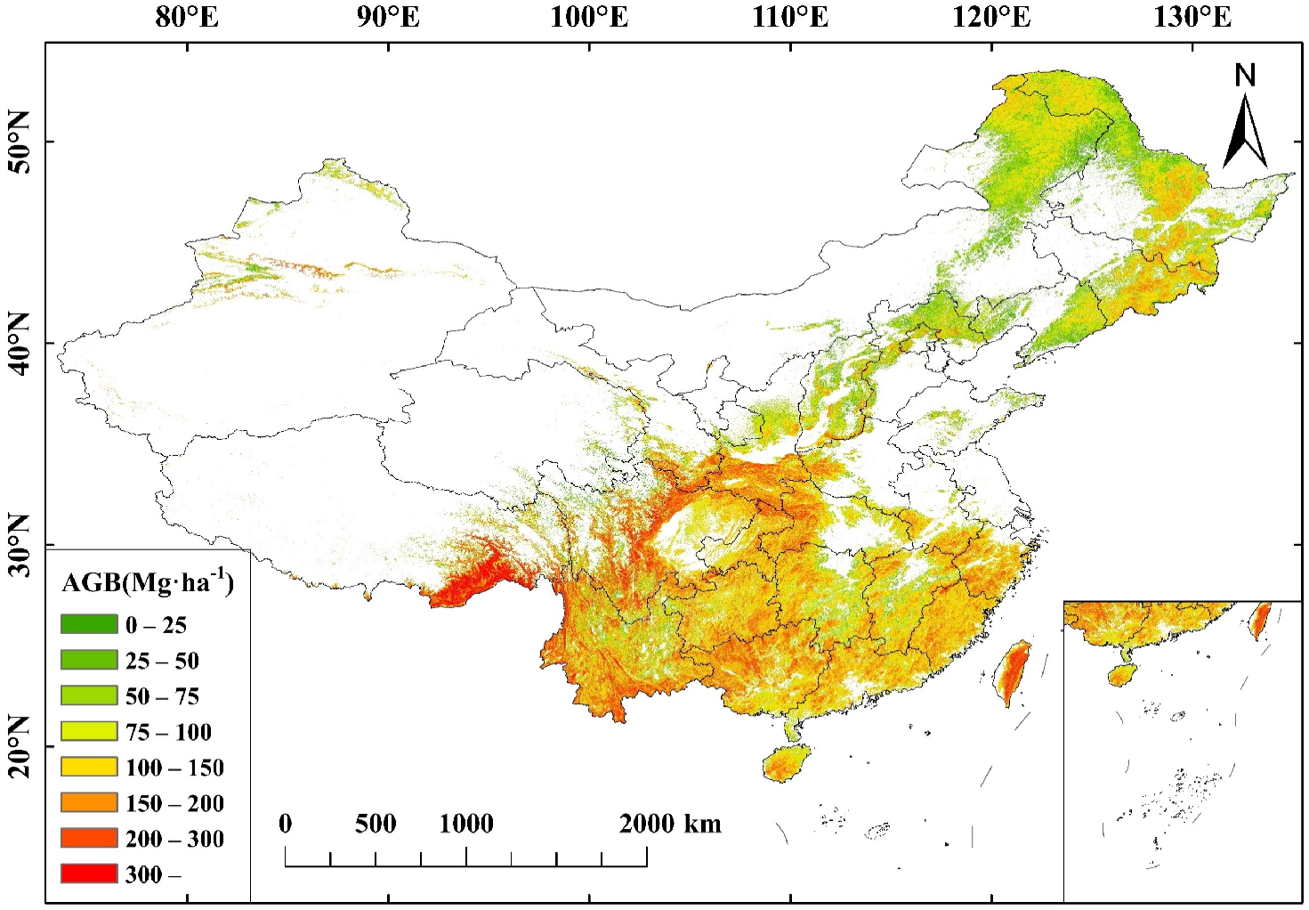
Using the Sentinel-2 imagery and terrain data, the 200 m resolution mean and standard deviation images were computed. These were input into the trained LightGBM model, along with calculated NDSI indices, to predict the AGB for each province. The resulting forest AGB distribution map is shown in Figure 10.

Figure 10 presents the predicted spatial distribution of China’s forest aboveground biomass (AGB) for 2022, with units in Mg·ha⁻¹. The average forest AGB across China is 123.90 Mg·ha⁻¹. Overall, the forest AGB exhibits clear spatial heterogeneity, with a pattern of higher values in the southeast and lower values in the northwest.

High-biomass areas (AGB > 200 Mg·ha⁻¹) are primarily concentrated in the mountainous and tropical regions of southwestern China, such as southern Yunnan, southeastern Tibet, Hainan Island, and the western edge of the Sichuan Basin. These areas are dominated by evergreen broadleaf forests or tropical rainforests characterized by warm and humid climates and mature forests with substantial biomass accumulation.

Moderate biomass density regions (100–200 Mg·ha⁻¹) are widely distributed across central and southern China as well as southern Northeast China, including provinces like Jiangxi, Hunan, Zhejiang, and southern Jilin. These regions mainly contain mixed coniferous and broadleaf forests and fast-growing plantations, with relatively intact forest structures and solid resource bases.

Low AGB regions (<75 Mg·ha⁻¹) are mainly found in the arid northwest and the Qinghai–Tibet Plateau interior, including Xinjiang, Gansu, Qinghai, and northwestern Tibet. These areas have harsh ecological conditions, sparse forest vegetation, and low productivity levels.

The distribution map also reveals notable transitional zones with moderate to low biomass (75–100 Mg·ha⁻¹) along the southern edge of the Northeast Plain, the Loess Plateau margins, and the Qinling–Huaihe ecological transition belt, reflecting typical ecological gradient changes.

The overall spatial pattern aligns well with China’s forest ecological zoning and climatic gradients and shows strong consistency with large-scale forest AGB estimates from previous studies, indicating that the model possesses good predictive capability and ecological plausibility at the national scale.

The overall spatial pattern aligns well with China’s forest ecological zoning and climatic gradients, indicating that the model captures the broad-scale ecological plausibility of forest biomass at the national level. Quantitative comparisons with previous studies are provided in Section 3.8.

3.7. Spatial Distribution of Prediction Uncertainty

The 95% prediction interval of forest AGB was calculated using the LightGBM-based quantile regression approach described in Section 2.5.4, in which two models were trained to predict the 2.5th and 97.5th percentiles of AGB. The uncertainty was quantified by the difference between the predicted upper and lower quantile values, based on which a national distribution map of forest AGB prediction uncertainty was generated (Figure 11).

Overall, the uncertainty in most forested areas across China ranges between 3 and 6 Mg·ha⁻¹, with only a few regions showing uncertainties below 3 Mg·ha⁻¹, indicating high overall prediction stability. Spatially, areas with lower uncertainty are mainly concentrated in the eastern plains, central parts of the northeastern forest region, and the middle to lower reaches of the Yangtze River. These regions have dense training samples, high-quality remote sensing imagery, and stable feature-response relationships, resulting in smaller prediction errors.

In contrast, regions with significantly higher uncertainty (>9 Mg·ha⁻¹) are mainly found in three types of areas: (1) Southwest mountainous canyon forests (e.g., western Sichuan, southwestern Yunnan), where complex terrain and severe land cover mixing cause large disturbances in spectral input features and reduce model responsiveness; (2) tropical seasonal rainforest regions (e.g., Hainan Island and Xishuangbanna), where local prediction uncertainty is elevated, likely due to extremely high biomass density and spectral saturation effects; (3) edges of the high-latitude northeastern forest zone, which exhibit clustered prediction uncertainties possibly related to strong forest heterogeneity and large variations in stand structure. Additionally, some areas without extreme terrain may have locally elevated uncertainties due to sparse training samples or fluctuations in remote sensing data quality.

In summary, this uncertainty map provides an intuitive spatial characterization of model confidence. It is recommended that structural remote sensing data sources (such as SAR and LiDAR) or regional sub-models be introduced preferentially in high-uncertainty areas to improve the reliability and accuracy of forest biomass inversion in complex terrain or high-biomass regions.

3.8. Accuracy Validation of Model Predictions

The predicted average forest AGB for China is 123.90 Mg·ha⁻¹, which shows a relative error of 3.25% compared to the national average reported by Su et al. [42] (120 Mg·ha⁻¹), and a relative error of 1.87% compared to the 2022 average AGB reported by Cai et al. [22] (121.62 Mg·ha⁻¹). The spatial distribution patterns are also highly consistent, with high biomass areas (exceeding 300 Mg·ha⁻¹) concentrated in southern Tibet, the Qinling Mountains, parts of Northeast China, and Taiwan, confirming the accuracy of the model predictions.

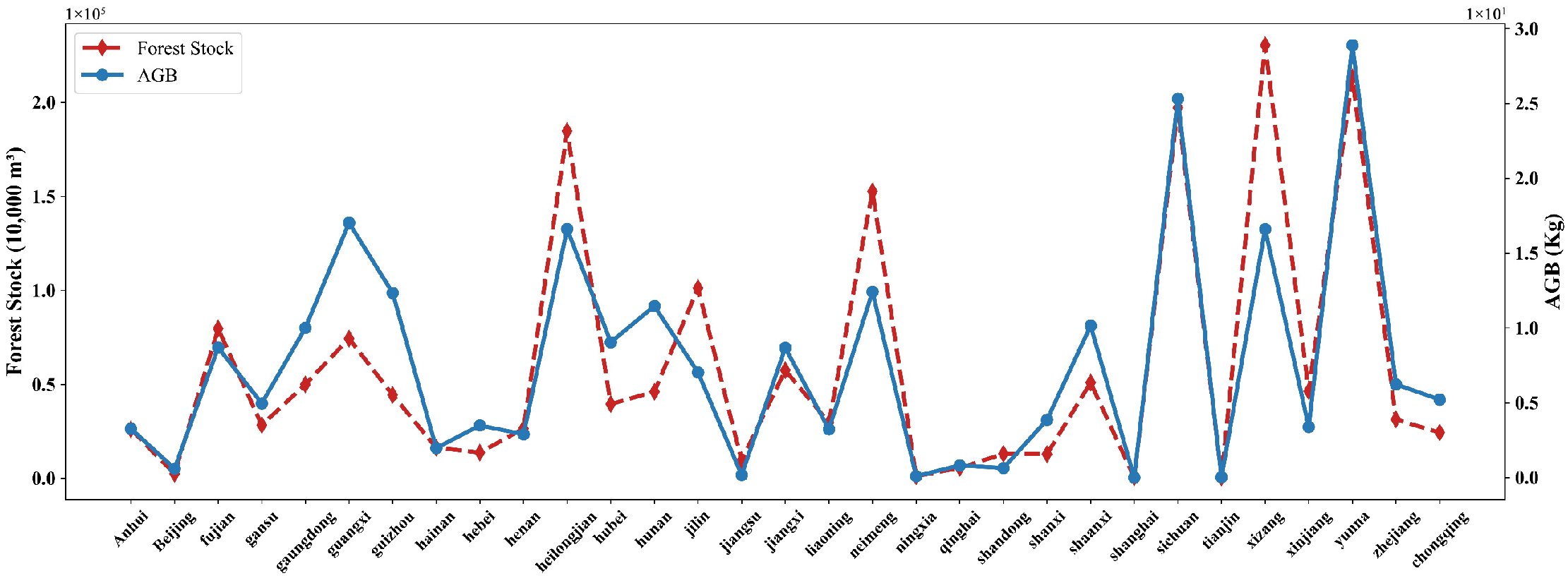
The Spearman rank correlation coefficient between the total provincial AGB predicted by the model and the forest stand volume reported in the China Statistical Yearbook is 0.88, indicating a strong agreement in the ranking of resource stocks at the provincial level (see Figure 12). The line chart comparing provincial forest AGB and forest stand volume is also shown in Figure 12. This close relationship further demonstrates the model’s reliable predictive capability at the national scale and supports the use of GEDI L4A products as a valid ground truth source for forest AGB inversion in China.

In summary, the three-tier validation results demonstrate that our predictions are accurate and reliable across multiple scales. The national-scale agreement test revealed less than 3.25% deviation from independent studies, ensuring overall unbiasedness; the regional-scale spatial pattern comparison confirmed the model’s reliability across diverse geographic regions; and the provincial-scale stock ranking correlation (ρ = 0.88) further verified the rationality of macro-scale resource distribution. Collectively, these results validate the accuracy and authenticity of our predictions, consistent with findings from existing continental-scale forest biomass studies.

4. Discussion

4.1. Model Performance and Comparison with Existing Methods

The LightGBM model developed in this study achieved a test set performance of R² = 0.76 and RMSE = 47.73 Mg·ha⁻¹, significantly outperforming conventional methods such as linear regression and support vector machines, and showing comparable accuracy to the national-scale AGB estimation results based on random forest by Su et al. (2016). Furthermore, by using GEDI L4A data as training labels, this study effectively overcomes the spatial heterogeneity of traditional forest inventory data, enabling better model generalization at the national scale.

Currently, most AGB inversion studies focus on accuracy improvement by integrating Landsat and Sentinel imagery, combining optical and SAR or optical time-series data, and applying deep learning methods to enhance model performance. While SAR and LiDAR data have proven effective in mitigating saturation effects of optical imagery, optical remote sensing remains indispensable in long-term forest AGB monitoring due to its extensive temporal coverage. Therefore, a thorough understanding of optical data saturation mechanisms and the compensatory role of topographic features is particularly crucial, which constitutes the core analytical focus of this study.

Although some progress has been made in improving accuracy, there is a lack of quantitative analysis and systematic exploration of the error structure related to optical saturation in high biomass regions. Previous studies, constrained by limited field measurements, have mostly focused on regional models [15,16,17,18] for inversion and saturation mechanism analysis, without conducting large-scale systematic assessments. Cai et al. [22] pioneered the use of GEDI data as reference to estimate nationwide forest AGB over long time series, but their study did not provide a detailed error mechanism analysis at the national scale, particularly a systematic quantification of optical saturation.

In contrast, this study constructs an optical-dominant forest AGB inversion model across China at 200 m resolution using GEDI L4A samples without incorporating SAR or LiDAR data. By integrating NDSI indices and topographic variables, it systematically quantifies the saturation mechanisms of optical imagery and the compensatory effect of terrain on optical saturation across the entire country. Through LOWESS response curves and stratified error analysis, multiple typical spectral features’ saturation thresholds were quantified, and key causes of model performance degradation in high AGB areas were identified. This analysis enriches the error interpretation dimension of optical inversion methods and provides theoretical support for subsequent models integrating optical and structural features.

Additionally, residuals were analyzed across biomass groups and provincial scales to examine the spatial distribution of prediction errors and potential overestimation. Although the overall R² is slightly lower than some regional studies, the model developed here demonstrates better generalization and interpretability across diverse terrains and forest types, making it more suitable for national-scale carbon stock remote sensing modeling tasks.

4.2. Spectral Index Saturation Response Mechanism

This section provides a detailed quantitative dissection of the optical saturation effect.

SHAP analysis (Figure 7) revealed that spectral variables, particularly band_B4_avg, band_B5_avg, and NDSI_B2_B4_avg, contributed substantially to the prediction of AGB, underscoring their relevance as key optical predictors. Previous studies have demonstrated that red-edge bands can effectively estimate carbon content in drought-affected forests [43], where carbon is predominantly stored in biomass, especially AGB. NDSIs derived from visible and red-edge bands have also been shown to reliably estimate crop yield and AGB [20,33].

The core of our saturation analysis lies in the stratified error analysis and LOWESS curve fitting. This study identified typical saturation response characteristics of optical indices in high AGB regions. The two primary spectral bands—band_B4_avg and band_B5_avg—entered a plateau around AGB ≈ 80 Mg·ha⁻¹, while NDSI_B2_B4_avg maintained a strong response up to 100–150 Mg·ha⁻¹. In contrast, NDSI_B11_B12_avg peaked at 100–150 Mg·ha⁻¹ and subsequently exhibited a negative slope. These response patterns indicate that spectral signals progressively lose sensitivity in medium-to-high biomass areas, especially beyond 200 Mg·ha⁻¹, where model RMSE increases and bias becomes significantly negative, reflecting that spectral saturation is a major driver of error escalation.

This phenomenon is attributable to saturation and loss of sensitivity of spectral indices under high Leaf Area Index (LAI) conditions. Previous studies have shown that when LAI exceeds 4–6, indices such as NDVI rapidly lose sensitivity, and spectral values no longer reflect true structural differences [44]. Additionally, in dense canopies, multiple scattering of sunlight within the canopy, particularly in the near-infrared and shortwave infrared bands, stabilizes reflectance, limiting the ability to resolve biomass variations [10]. Therefore, although NDSI-type composite indices can enhance discrimination in moderate AGB ranges, their effectiveness degrades severely at high AGB levels, exhibiting non-monotonic responses.

4.3. Compensation Mechanism of Topographic and Spatial Structure Variables

Following the quantification of saturation, we further investigated the compensatory role of topographic variables.

SHAP interpretation also highlighted the strong contributions of topographic variables such as slope_avg and dem_std, indicating their essential role in improving prediction performance by capturing spatial heterogeneity and terrain effects. Additionally, DEM and derived terrain parameters help elucidate the influence of topography on local growth conditions, thereby revealing spatial patterns of biomass distribution [13]. Among topographic variables, slope exerts a notable influence on prediction results, which may be linked to errors in GEDI algorithm estimates in steep terrain areas. In such regions, GEDI might misestimate terrain and tree heights [31], while slope can mitigate the indirect propagation of lidar errors into prediction accuracy.

Combined SHAP analysis (Figure 7) and LOWESS curves (Figure 8c,f) indicate that topographic features (slope_avg and dem_std) maintain a relatively stable positive contribution when AGB is below 300 Mg·ha⁻¹. They can continuously provide information related to forest structure and site productivity when spectral variables experience saturation, partially compensating for the increased uncertainty caused by the loss of optical information. However, in regions where AGB exceeds 300 Mg·ha⁻¹, both features show declining response trends, suggesting that the compensatory effects of topographic variables also diminish in extremely high-biomass areas, which aligns with and explains the error patterns observed in Section 4.2.

Topographic factors indirectly reflect ecological attributes such as site conditions and habitat heterogeneity, thereby mitigating uncertainty caused by loss of optical information and indirectly influencing forest growth structure and carbon storage [45]. For example, elevation controls several key environmental variables [13]: (1) atmospheric pressure; (2) adiabatic temperature lapse rates; (3) clear-sky radiation; and (4) the proportion of ultraviolet radiation in solar irradiance. These factors influence forest growing season length, accumulated temperature, photosynthetic potential, and nutrient availability [46]. Elevation is a principal driver of temperature-related growth conditions [13], and topographically modulated variables such as potential incoming solar radiation improve biomass modeling by providing fine-scale energy input heterogeneity [47]. Areas with differing slope and aspect can have markedly different subsurface and surface temperatures and plant growth conditions [48].

Thus, topographic information can assist biomass modeling, especially in complex terrain where solar incidence angles and surface undulations increase noise in purely optical indices. Here, topographic variables act as stabilizing compensators. Additionally, GEDI data are known to have waveform distortion issues in areas with slope >25° [31]; incorporating topographic variables helps to mitigate indirect propagation of LiDAR errors in steep terrain during prediction.

Based on the results of this study, although the response of topographic variables weakens in areas with high aboveground biomass (>300 Mg·ha⁻¹), these variables still play a crucial auxiliary role in the biomass inversion model by serving as proxies for environmental heterogeneity and compensating for limitations in optical data.

Nevertheless, in areas with extreme terrain or sparse samples, such as the mountainous region of Chongqing, the model still exhibits systematic underestimation. This indicates that although topographic features have compensatory capacity, they cannot fully substitute for canopy structure information. Future work could enhance structural sensitivity in high-biomass regions by integrating multi-source remote sensing data, such as P-band microwave or full-waveform LiDAR, thereby further improving model robustness under complex terrain conditions caused by saturation.

4.4. Spatial Residual Distribution and Identification of Uncertainty Regions

The prediction residuals in this study exhibit significant spatial heterogeneity. Systematic underestimation is observed in regions such as Chongqing and Inner Mongolia, whereas slight overestimation occurs in eastern provinces including Jiangsu, Jiangxi. The spatial variation in residuals can be partly explained by (1) complex mountainous terrain causing degradation in GEDI LiDAR echo quality, which leads to larger reference data errors, and (2) uneven distribution of training samples in these regions, weakening model generalization and reducing its ability to capture local feature variations effectively. Moreover, forest type heterogeneity induces spectral response shifts, especially in mixed and conifer–broadleaf mixed forests where canopy structure and leaf morphology differ, resulting in partial decoupling from principal spectral indices. In eastern and southern provinces, overestimation may also be related to differences in forest types, higher surface reflectance, or sample structure imbalance, particularly where spectral characteristics of some plantation forests differ from the dominant training samples. Future work should enhance sample coverage in regions with sparse data, adopt regional stratified modeling strategies, and incorporate multi-source remote sensing data to further improve prediction accuracy in complex terrains and ecologically heterogeneous areas.

4.5. Impact of GEDI L4A Data Errors

This study employs the GEDI L4A product as the reference AGB dataset for model training and validation, offering global coverage with relatively uniform spatial distribution of high-resolution AGB estimates [20,22]. However, it is critical to acknowledge that GEDI L4A is not an error-free “ground truth” and its accuracy varies regionally. Previous research has highlighted that GEDI prediction models exhibit reduced accuracy in Asia [49], particularly in complex terrain (e.g., steep slopes) and high-AGB forests. For example, Liu et al. [31] reported significantly increased errors in terrain and tree height retrievals in areas with slopes >25°, while Duncanson et al. [49] noted potential regional systematic biases due to limited training data representativeness in Asia.

In this study, significant systematic underestimation (negative bias) occurs in the high AGB range (>300 Mg·ha⁻¹) (Table 6, Figure 6), partially attributable to spectral saturation effects of Sentinel-2 optical imagery (as discussed in Section 4.2). Simultaneously, we cannot exclude the possibility that GEDI L4A reference values themselves exhibit systematic underestimation in complex terrain and high-biomass forests in southwest China, thereby partially contributing to the observed negative model bias. The observed negative bias relative to GEDI arises from the combined effects of model error (including optical saturation) and GEDI reference error.

To mitigate GEDI errors’ impact, strict quality control was applied in preprocessing, including filtering out samples with excessive slope and relative errors, and adopting grid-based aggregation to smooth random geolocation errors (~±10 m) and individual AGB estimation uncertainties.

Despite these measures, potential systematic biases in GEDI L4A may remain in certain regions. Nonetheless, the core mechanisms revealed herein—the saturation response of optical spectral signals in high AGB areas and the compensatory role of topographic features—are strongly supported by both mechanistic reasoning and data evidence.

First, the nonlinear relationship between input features and model responses exhibits physical plausibility: as shown in Figure 7, red and red-edge reflectances (B4, B5) plateau near 100 Mg·ha⁻¹, and vegetation indices such as NDSI weaken or invert responses beyond 100–150 Mg·ha⁻¹, consistent with extensive spectral saturation literature [10,17,18], unlikely to be solely driven by GEDI errors.

Secondly, topographic features such as slope_avg and dem_std demonstrate high importance in the SHAP analysis and maintain stable, positive predictive contributions in the medium- to high-AGB range (<300 Mg·ha⁻¹) according to the LOWESS curves, without showing obvious plateauing or reversal. This suggests that their compensatory effect operates independently of GEDI accuracy within this range and more likely reflects their indirect explanatory power of forest site conditions. However, in extremely high AGB regions, this trend weakens, indicating that the compensatory effect also has its limits.

Finally, stratified error statistics (Table 6, Figure 6) show systematic negative bias in high-AGB regions with spectral saturation, rather than an overall increase in random errors, further supporting the saturation mechanism.

In summary, despite GEDI accuracy limitations in some areas, the findings on optical saturation thresholds, error distribution patterns, and topographic compensation mechanisms are robust, grounded in reproducible and physically meaningful relationships between model inputs and outputs. While GEDI errors may partially contribute to negative bias, the spectral saturation features (Figure 8a,d) and stable topographic compensation (Figure 8c,f) are independent of reference data and aligned with physical theory, confirming spectral saturation as the primary source of high-AGB prediction errors.

4.6. Future Work

• Integrate Higher-Accuracy Reference Data: Collect extensive airborne LiDAR data or high-precision field plot measurements in representative Chinese forest types—especially high-AGB areas—to directly validate and calibrate GEDI L4A accuracy and bias, providing more reliable reference data for pure analysis of optical saturation effects.
• Develop Regional GEDI Correction Models: Using newly acquired high-accuracy reference data, establish correction models tailored for China’s major forest ecological zones to reduce systematic GEDI L4A biases before large-scale modeling and analysis.
• Explore Multi-Source Data Fusion: Investigate combining other spaceborne LiDAR (e.g., ICESat-2 ATL08) or SAR datasets (e.g., L-band ALOS-2/PALSAR-2, C-band Sentinel-1) to supply structural information that complements or substitutes GEDI, thereby directly alleviating optical saturation issues, especially where GEDI coverage is limited or uncertain.
• Regional and Forest-Type Specific Modeling: Conduct province-level or forest-type (coniferous, broadleaf, mixed) sub-model training and mechanism analyses to better capture regional GEDI error patterns and spectral saturation response heterogeneity.

5. Conclusions

This study developed a nationwide forest aboveground biomass (AGB) inversion model at 200 m resolution based on GEDI L4A samples and Sentinel-2 optical remote sensing imagery. The model integrates normalized difference spectral indices (NDSI) and topographic variables, achieving relatively stable predictive performance (R² = 0.75, RMSE = 44.28 Mg·ha⁻¹). It further focuses on the prediction error structure and spectral saturation mechanisms in high-biomass areas through systematic analysis.

The main conclusions are as follows:

• In high AGB regions exceeding 300 Mg·ha⁻¹, model prediction accuracy significantly deteriorates, with notable increases in RMSE and negative bias, indicating a saturation response in spectral input features.
• Response curve analysis revealed that single-band reflectances (e.g., B4, B5) reach a plateau around 80 Mg·ha⁻¹, whereas NDSI-type indices delay the saturation threshold to approximately 100–150 Mg·ha⁻¹. Some indices (e.g., NDSI_B11_B12) even exhibit inverse response trends in high AGB zones, further illustrating signal degradation.
• Topographic structural features such as slope and DEM variability maintain stable contributions below 300 Mg·ha⁻¹ and can partially compensate for the loss of predictive information caused by spectral saturation; however, they cannot fully offset the systematic underestimation observed in dense forest areas.
• Through stratified error analysis and threshold quantification based on LOWESS response curves, this study provides an empirical assessment of the performance limits of optical AGB inversion models at the national scale, offering a theoretical basis for future integration of SAR, LiDAR data, or the development of regionalized models.

In summary, this work not only produces a high-resolution, nationwide forest AGB data product but also mechanistically reveals the limitations and applicability boundaries of optical remote sensing-based AGB inversion. It offers important insights for improving model interpretability and advancing fusion methodologies. The methods and analytical framework presented here can be directly applied to forest AGB inversion in other countries, providing technical reference for global carbon stock assessment and climate change research.

References

1. Pan, Y.; Birdsey, R.A.; Fang, J.; Houghton, R.; Kauppi, P.E.; Kurz, W.A.; Phillips, O.L.; Shvidenko, A.; Lewis, S.L.; Canadell, J.G.; et al. A Large and Persistent Carbon Sink in the World’s Forests. Science 2011, 333, 988–993. [Google Scholar] [CrossRef]
2. Piao, S.; Fang, J.; He, J.; Xiao, Y. Biomass and Its Spatial Distribution Pattern of Grassland Vegetation in China. Chin. J. Plant Ecol. 2004, 28, 491–498. [Google Scholar]
3. Tian, L.; Wu, X.; Tao, Y.; Li, M.; Qian, C.; Liao, L.; Fu, W. Review of Remote Sensing-Based Methods for Forest Aboveground Biomass Estimation: Progress, Challenges, and Prospects. Forests 2023, 14, 1086. [Google Scholar] [CrossRef]
4. Yu, Y.; Saatchi, S.; Heath, L.S.; LaPoint, E.; Myneni, R.; Knyazikhin, Y. Regional distribution of forest height and biomass from multisensor data fusion. J. Geophys. Res. Biogeosciences 2010, 115, G00E12. [Google Scholar] [CrossRef]
5. Urbazaev, M.; Thiel, C.; Cremer, F.; Dubayah, R.; Migliavacca, M.; Reichstein, M.; Schmullius, C. Estimation of forest aboveground biomass and uncertainties by integration of field measurements, airborne LiDAR, and SAR and optical satellite data in Mexico. Carbon Balance Manag. 2018, 13, 5. [Google Scholar] [CrossRef]
6. Avitabile, V.; Baccini, A.; Friedl, M.A.; Schmullius, C. Capabilities and limitations of Landsat and land cover data for aboveground woody biomass estimation of Uganda. Remote Sens. Environ. 2012, 117, 366–380. [Google Scholar] [CrossRef]
7. Wang, M.; Fan, L.; Frappart, F.; Ciais, P.; Sun, R.; Liu, Y.; Li, X.; Liu, X.; Moisy, C.; Wigneron, J.-P. An alternative AMSR2 vegetation optical depth for monitoring vegetation at large scales. Remote Sens. Environ. 2021, 263, 112556. [Google Scholar] [CrossRef]
8. Fan, L.; Wigneron, J.-P.; Ciais, P.; Chave, J.; Brandt, M.; Fensholt, R.; Saatchi, S.S.; Bastos, A.; Al-Yaari, A.; Hufkens, K.; et al. Satellite-observed pantropical carbon dynamics. Nat. Plants 2019, 5, 944–951. [Google Scholar] [CrossRef]
9. Chang, Z.; Fan, L.; Wigneron, J.-P.; Wang, Y.-P.; Li, X.; Wang, M.; Liu, X.; Wang, H.; Cui, T.; Yu, L.; et al. Evaluation of optical and microwave-derived vegetation indices for monitoring aboveground biomass over China. Geo-Spat. Inf. Sci. 2025, 28, 421–436. [Google Scholar] [CrossRef]
10. Mutanga, O.; Masenyama, A.; Sibanda, M. Spectral saturation in the remote sensing of high-density vegetation traits: A systematic review of progress, challenges, and prospects. ISPRS J. Photogramm. Remote Sens. 2023, 198, 297–309. [Google Scholar] [CrossRef]
11. Zeng, P.; Zhang, W.; Li, Y.; Shi, J.; Wang, Z. Forest Total and Component Above-Ground Biomass (AGB) Estimation through C- and L-band Polarimetric SAR Data. Forests 2022, 13, 442. [Google Scholar] [CrossRef]
12. Li, W.; Zhang, Y.; Zhang, J.; Chen, H.; Chen, E.; Zhao, L.; Zhao, D. Tropical forest AGB estimation based on structure parameters extracted by TomoSAR. Int. J. Appl. Earth Obs. Geoinf. 2023, 121, 103369. [Google Scholar] [CrossRef]
13. Riihimäki, H.; Heiskanen, J.; Luoto, M. The effect of topography on arctic-alpine aboveground biomass and NDVI patterns. Int. J. Appl. Earth Obs. Geoinf. 2017, 56, 44–53. [Google Scholar] [CrossRef]
14. McEwan, R.W.; Lin, Y.-C.; Sun, I.-F.; Hsieh, C.-F.; Su, S.-H.; Chang, L.-W.; Song, G.-Z.M.; Wang, H.-H.; Hwong, J.-L.; Lin, K.-C.; et al. Topographic and biotic regulation of aboveground carbon storage in subtropical broad-leaved forests of Taiwan. For. Ecol. Manag. 2011, 262, 1817–1825. [Google Scholar] [CrossRef]
15. Sa, R.; Nie, Y.; Chumachenko, S.; Fan, W. Biomass Estimation and Saturation Value Determination Based on Multi-Source Remote Sensing Data. Remote Sens. 2024, 16, 2250. [Google Scholar] [CrossRef]
16. Wu, Y.; Guo, B.; Zhang, X.; Luo, H.; Yu, Z.; Li, H.; Shi, K.; Wang, L.; Xu, W.; Ou, G. Response of Hydrothermal Conditions to the Saturation Values of Forest Aboveground Biomass Estimation by Remote Sensing in Yunnan Province, China. Land 2024, 13, 1534. [Google Scholar] [CrossRef]
17. Wu, S.; Sun, Y.; Jia, W.; Wang, F.; Lu, S.; Zhao, H. Estimation of Above-Ground Carbon Storage and Light Saturation Value in Northeastern China’s Natural Forests Using Different Spatial Regression Models. Forests 2023, 14, 1970. [Google Scholar] [CrossRef]
18. Zhao, P.; Lu, D.; Wang, G.; Wu, C.; Huang, Y.; Yu, S. Examining Spectral Reflectance Saturation in Landsat Imagery and Corresponding Solutions to Improve Forest Aboveground Biomass Estimation. Remote Sens. 2016, 8, 469. [Google Scholar] [CrossRef]
19. Zhang, R.; Zhou, X.; Ouyang, Z.; Avitabile, V.; Qi, J.; Chen, J.; Giannico, V. Estimating aboveground biomass in subtropical forests of China by integrating multisource remote sensing and ground data. Remote Sens. Environ. 2019, 232, 111341. [Google Scholar] [CrossRef]
20. Shendryk, Y. Fusing GEDI with earth observation data for large area aboveground biomass mapping. Int. J. Appl. Earth Obs. Geoinf. 2022, 115, 103108. [Google Scholar] [CrossRef]
21. Sialelli, G.; Peters, T.; Wegner, J.D.; Schindler, K. AGBD: A Global-scale Biomass Dataset. arXiv 2024, arXiv:2406.04928. [Google Scholar] [CrossRef]
22. Cai, Y.; Zhu, P.; Li, X.; Liu, X.; Chen, Y.; Shen, Q.; Xu, X.; Zhang, H.; Nie, S.; Wang, C.; et al. Dynamics of China’s Forest Carbon Storage: The First 30 m Annual Aboveground Biomass Mapping from 1985 to 2023. Earth Syst. Sci. Data 2025, 1–34, Preprint. [Google Scholar] [CrossRef]
23. National Bureau of Statistics of China. China Statistical Yearbook—2023. Available online: https://www.stats.gov.cn/sj/ndsj/2023/indexch.htm (accessed on 1 September 2024).
24. Tianditu Cloud Center. Administrative Division Service. Available online: https://cloudcenter.tianditu.gov.cn/administrativeDivision (accessed on 5 September 2024).
25. Yang, J.; Huang, X. The 30 m annual land cover dataset and its dynamics in China from 1990 to 2019. Earth Syst. Sci. Data 2021, 13, 3907–3925. [Google Scholar] [CrossRef]
26. Main-Knorn, M.; Pflug, B.; Louis, J.; Debaecker, V.; Müller-Wilm, U.; Gascon, F. Sen2Cor for Sentinel-2. In Proceedings of the Image and Signal Processing for Remote Sensing XXIII, Warsaw, Poland, 11–13 September 2017; SPIE: Bellingham, WA, USA, 2017; Volume 10427, pp. 37–48. [Google Scholar]
27. Dubayah, R.; Blair, J.B.; Goetz, S.; Fatoyinbo, L.; Hansen, M.; Healey, S.; Hofton, M.; Hurtt, G.; Kellner, J.; Luthcke, S.; et al. The Global Ecosystem Dynamics Investigation: High-resolution laser ranging of the Earth’s forests and topography. Sci. Remote Sens. 2020, 1, 100002. [Google Scholar] [CrossRef]
28. Wang, C.; Zhang, W.; Ji, Y.; Marino, A.; Li, C.; Wang, L.; Zhao, H.; Wang, M. Estimation of Aboveground Biomass for Different Forest Types Using Data from Sentinel-1, Sentinel-2, ALOS PALSAR-2, and GEDI. Forests 2024, 15, 215. [Google Scholar] [CrossRef]
29. Kanmegne Tamga, D.; Latifi, H.; Ullmann, T.; Baumhauer, R.; Bayala, J.; Thiel, M. Estimation of Aboveground Biomass in Agroforestry Systems over Three Climatic Regions in West Africa Using Sentinel-1, Sentinel-2, ALOS, and GEDI Data. Sensors 2023, 23, 349. [Google Scholar] [CrossRef]
30. Zurqani, H.A. A multi-source approach combining GEDI LiDAR, satellite data, and machine learning algorithms for estimating forest aboveground biomass on Google Earth Engine platform. Ecol. Inform. 2025, 86, 103052. [Google Scholar] [CrossRef]
31. Liu, A.; Cheng, X.; Chen, Z. Performance evaluation of GEDI and ICESat-2 laser altimeter data for terrain and canopy height retrievals. Remote Sens. Environ. 2021, 264, 112571. [Google Scholar] [CrossRef]
32. Shendryk, Y.; Rossiter-Rachor, N.A.; Setterfield, S.A.; Levick, S.R. Leveraging High-Resolution Satellite Imagery and Gradient Boosting for Invasive Weed Mapping. IEEE J. Sel. Top. Appl. Earth Obs. Remote Sens. 2020, 13, 4443–4450. [Google Scholar] [CrossRef]
33. Shendryk, Y.; Davy, R.; Thorburn, P. Integrating satellite imagery and environmental data to predict field-level cane and sugar yields in Australia using machine learning. Field Crops Res. 2021, 260, 107984. [Google Scholar] [CrossRef]
34. Roy, D.P.; Kashongwe, H.B.; Armston, J. The impact of geolocation uncertainty on GEDI tropical forest canopy height estimation and change monitoring. Sci. Remote Sens. 2021, 4, 100024. [Google Scholar] [CrossRef]
35. Ke, G.; Meng, Q.; Finley, T.; Wang, T.; Chen, W.; Ma, W.; Ye, Q.; Liu, T.-Y. LightGBM: A Highly Efficient Gradient Boosting Decision Tree. In Proceedings of the 31st International Conference on Neural Information Processing Systems, Long Beach, CA, USA, 4–9 December 2017; Curran Associates, Inc.: Red Hook, NY, USA, 2017; Volume 30. [Google Scholar]
36. Huang, X.; Cheng, F.; Wang, J.; Duan, P.; Wang, J. Forest Canopy Height Extraction Method Based on ICESat-2/ATLAS Data. IEEE Trans. Geosci. Remote Sens. 2023, 61, 1–14. [Google Scholar] [CrossRef]
37. Sang, M.; Xiao, H.; Jin, Z.; He, J.; Wang, N.; Wang, W. Improved Mapping of Regional Forest Heights by Combining Denoise and LightGBM Method. Remote Sens. 2023, 15, 5436. [Google Scholar] [CrossRef]
38. Rahmati, O.; Choubin, B.; Fathabadi, A.; Coulon, F.; Soltani, E.; Shahabi, H.; Mollaefar, E.; Tiefenbacher, J.; Cipullo, S.; Bin Ahmad, B.; et al. Predicting uncertainty of machine learning models for modelling nitrate pollution of groundwater using quantile regression and UNEEC methods. Sci. Total Environ. 2019, 688, 855–866. [Google Scholar] [CrossRef] [PubMed]
39. Kasraei, B.; Heung, B.; Saurette, D.D.; Schmidt, M.G.; Bulmer, C.E.; Bethel, W. Quantile regression as a generic approach for estimating uncertainty of digital soil maps produced from machine-learning. Environ. Model. Softw. 2021, 144, 105139. [Google Scholar] [CrossRef]
40. Wen, X.; Xie, Y.; Wu, L.; Jiang, L. Quantifying and comparing the effects of key risk factors on various types of roadway segment crashes with LightGBM and SHAP. Accid. Anal. Prev. 2021, 159, 106261. [Google Scholar] [CrossRef]
41. Lundberg, S.; Lee, S.-I. A Unified Approach to Interpreting Model Predictions. arXiv 2017, arXiv:1705.07874. [Google Scholar] [CrossRef]
42. Su, Y.; Guo, Q.; Xue, B.; Hu, T.; Alvarez, O.; Tao, S.; Fang, J. Spatial distribution of forest aboveground biomass in China: Estimation through combination of spaceborne lidar, optical imagery, and forest inventory data. Remote Sens. Environ. 2016, 173, 187–199. [Google Scholar] [CrossRef]
43. Gara, T.W.; Murwira, A.; Ndaimani, H. Predicting forest carbon stocks from high resolution satellite data in dry forests of Zimbabwe: Exploring the effect of the red-edge band in forest carbon stocks estimation. Geocarto Int. 2016, 31, 176–192. [Google Scholar] [CrossRef]
44. Avitabile, V.; Herold, M.; Henry, M.; Schmullius, C. Mapping biomass with remote sensing: A comparison of methods for the case study of Uganda. Carbon Balance Manag. 2011, 6, 7. [Google Scholar] [CrossRef]
45. de Castilho, C.V.; Magnusson, W.E.; de Araújo, R.N.O.; Luizão, R.C.; Luizão, F.J.; Lima, A.P.; Higuchi, N. Variation in aboveground tree live biomass in a central Amazonian Forest: Effects of soil and topography. For. Ecol. Manag. 2006, 234, 85–96. [Google Scholar] [CrossRef]
46. Karlsson, S. Plant Ecology, Herbivory, and Human Impact in Nordic Mountain Birch Forests, 1st ed.; Ecological Studies; Springer: Berlin/Heidelberg, Germany, 2005; ISBN 978-3-540-22909-4. [Google Scholar]
47. Austin, M.P.; Van Niel, K.P. Improving species distribution models for climate change studies: Variable selection and scale. J. Biogeogr. 2011, 38, 1–8. [Google Scholar] [CrossRef]
48. Mod, H.K.; Scherrer, D.; Luoto, M.; Guisan, A. What we use is not what we know: Environmental predictors in plant distribution models. J. Veg. Sci. 2016, 27, 1308–1322. [Google Scholar] [CrossRef]
49. Duncanson, L.; Kellner, J.R.; Armston, J.; Dubayah, R.; Minor, D.M.; Hancock, S.; Healey, S.P.; Patterson, P.L.; Saarela, S.; Marselis, S.; et al. Aboveground biomass density models for NASA’s Global Ecosystem Dynamics Investigation (GEDI) lidar mission. Remote Sens. Environ. 2022, 270, 112845. [Google Scholar] [CrossRef]
Figure 1. Study area of China.
Remotesensing 17 03437 g001
Figure 2. Workflow of national-scale forest AGB mapping and spectral saturation mechanism analysis, including data preprocessing, grid aggregation, feature extraction, modeling, and saturation mechanism analysis.
Remotesensing 17 03437 g002
Figure 3. Spatial distribution of quality-filtered GEDI L4A footprints (2022) within forested areas of Shanxi Province. Forest mask data are derived from the CLCD dataset (2022).
Remotesensing 17 03437 g003
Figure 4. Data distribution before and after balancing the AGB samples.
Remotesensing 17 03437 g004
Figure 5. Scatter density plots of predicted versus observed AGB on the test set. (a) Model including topographic features; (b) model excluding topographic features.
Remotesensing 17 03437 g005
Figure 6. Line plots of RMSE (blue) and Bias (red) for the same model, stratified by AGB intervals.
Remotesensing 17 03437 g006
Figure 7. Mean absolute SHAP values and their distributions for the top 20 important features in the LightGBM model.
Remotesensing 17 03437 g007
Figure 8. LOWESS response curves illustrating the relationship between GEDI aboveground biomass (AGB) and selected spectral and topographic variables. Vertical dashed lines indicate approximate saturation thresholds at 80 Mg·ha−1 for single spectral bands, 100–150 Mg·ha−1 for NDSI-type indices, and around 300 Mg·ha−1 for topographic variables (DEM and slope). Subfigures: (a) Response of band_B4_avg to AGB; (b) Response of NDSI_B2_B4_avg to AGB; (c) Response of dem_std to AGB; (d) Response of band_B5_avg to AGB; (e) Response of NDSI_B11_B12_avg to AGB; (f) Response of slope_avg to AGB.
Remotesensing 17 03437 g008
Figure 9. Province-level residual heatmap across China at the national scale.
Remotesensing 17 03437 g009
Figure 10. AGB map of China in 2022.
Remotesensing 17 03437 g010
Figure 11. Spatial distribution of forest AGB prediction uncertainty across China: estimated using the 95% prediction interval derived from LightGBM quantile regression, reflecting spatial stability of the estimates.
Remotesensing 17 03437 g011
Figure 12. Comparison between provincial-level total forest aboveground biomass (AGB) predicted by the model and forest stand volume statistics from the China Statistical Yearbook (2022). The strong Spearman correlation coefficient (0.88) indicates high consistency between predicted AGB and reported stand volume across provinces.
Remotesensing 17 03437 g012