Spatial Sampling Uncertainty for MODIS Terra Land Surface Temperature Retrievals

Highlights

What are the main findings?

• A spatial sampling uncertainty model is developed for coarsening 1 km MODIS Terra land surface temperature satellite products to resolutions of 0.05° or 0.1°.
• Sampling uncertainty for land surface temperature is dependent on both the underlying land cover and the solar zenith angle at the time of observation.

What is the implication of the main finding?

• The largest sampling uncertainties occur in regions of mixed land cover at 0.05° and for urban areas at 0.1° and the shape of the spatial sampling uncertainty curve with clear-sky fraction differs from previous parameterisations.
• The spatial sampling uncertainty parameterisations presented here can be applied to MODIS Terra LST products and LST products from other morning overpass satellites with similar noise characteristics and spatial resolution.

Abstract

Land surface temperature (LST) data are often required at coarser resolutions than the native satellite data for user applications. LST products from infrared sensors are clear-sky only, and thus, coarsening such data introduces a sampling uncertainty where the target domain is not fully sampled. In this manuscript, we calculate sampling uncertainty as a function of clear-sky fraction for 0.01° products re-gridded to 0.05° and 0.1°. We find that sampling uncertainty is dependent on both the underlying land cover (biome) and the solar geometry at the time of the observation. The largest sampling uncertainties are seen for mixed pixels (encompassing a variety of biomes) at 0.05° resolution (0.98 K) and for urban pixels at 0.1° resolution (2.5 K). The spatial sampling uncertainty methodology presented here is applicable to any infrared LST products provided at these resolutions (from a native resolution of 0.01°/~1 km), irrespective of retrieval algorithm or satellite, provided that the uncertainty due to noise can be removed.

1. Introduction

The production of essential climate variable (ECV) [1] data records using satellite data has expanded rapidly in recent years [2,3,4,5,6,7,8,9]. There has been a growing recognition that providing per-observation uncertainty estimates is essential to facilitating good decision-making when applying these data in a climate context [10,11,12]. Methods have been developed to construct comprehensive uncertainty budgets from satellite retrievals, which take the measurement equation for the retrieval and break it down into its constituent components (e.g., different satellite inputs and auxiliary information). The error effects associated with each term are then identified [12,13]. Where possible, the uncertainty associated with each error effect is quantified, and together, these can be used to construct the uncertainty budget for the measurement [5,14,15].

Some aspects of the retrieval process, e.g., pre-processing steps such cloud detection, geolocation or sub-sampling, cannot be directly attributed to any of the individual input terms in the retrieval equation [12]. The ‘+0 term’ has been adopted in some publications as an addition to the measurement equation to denote these error effects. Efforts have been made to quantify them for inclusion in uncertainty budgets when constructing climate data records (CDRs) [12,16]. One such component that is common to many ECVs is the spatial sampling uncertainty that occurs when re-gridding high-resolution, spatially incomplete data onto coarser resolution grids [17,18]. Temporal sampling uncertainty also occurs when temporally incomplete products are averaged in time, e.g., daily, monthly, and annually, but the focus of this publication is on spatial sampling uncertainty for coarser-resolution products at the time of the satellite overpass.

In the context of land surface temperature (LST) products generated from infrared satellite data, spatial sampling uncertainty occurs because of cloud obscuring the Earth’s surface. In the presence of cloud, a surface temperature retrieval is not possible [3,16,19] (the retrieved temperature would be entirely or in part that of the cloud, depending on its opacity), which results in ‘gappy’ high-resolution data [2]. Users typically prefer working with regularly gridded products, often at a coarser resolution than the native satellite data [20]. In averaging the data to provide these products, sampling uncertainty occurs when subsampling the target domain due to partial cloud cover [17]. Note that these coarsened products, although spatially complete, represent a clear-sky LST, i.e., there is no knowledge of the temperature under clouds in these products.

A method for calculating spatial sampling uncertainty for surface temperature products has been previously developed and applied to sea surface temperature (SST) data [17]. A model for this uncertainty component was constructed by taking a large volume of clear-sky data and subsampling this by applying realistic cloud masks [18]. The SST differences between the subsampled and fully sampled cases provides the means to quantify the sampling uncertainty. This uncertainty is dependent on factors such as clear-sky fraction and, in the case of SST, the underlying SST variability in the subsampled data [18]. This paper applies this methodology to LST using data from the Moderate-Resolution Imaging Spectroradiometer (MODIS) to quantify sampling uncertainty at resolutions of 0.05° and 0.1°, as part of the European Space Agency (ESA) LST Climate Change Initiative (CCI) Project [4]. The land case is more complex than that of the ocean due to the greater heterogeneity of the land surface [3,16] and the diversity of land cover classes [21]. This means that the spatial sampling uncertainty algorithm requires adaptation for use with these products. Greater heterogeneity in land surface increases the likelihood that sampling uncertainty will depend on location and solar geometry.

The remainder of the paper is structured as follows: In Section 2, we discuss the MODIS data and sampling uncertainty methodology. Section 3 contains the sampling uncertainty results, including the dependence of sampling uncertainty on land cover, latitude, and solar zenith angle. For ‘mixed’ pixels, where <95% of the area comprises a single biome, we evaluate the impact of the number of land covers present and the percentage of the grid cell represented by the dominant biome on the sampling uncertainty. In Section 4, we discuss a strategy for applying these findings to LST CCI products and identify the remaining gaps in the parameterization of sampling uncertainty in gridded products. We conclude the paper in Section 5.

2. Data and Methods

2.1. Satellite Data Extraction

Land surface temperature (LST) products from polar-orbiting satellite missions are routinely provided at a resolution of 0.01° by the ESA LST CCI project. These data are Level 3 (L3) products, reprojected from the native image grid of the satellite onto a regular grid in latitude and longitude space. At the request of data users [20], these high-resolution L3 products are provided in preference to native-resolution Level 2 (L2) products on the native image grid and form the starting point for this study. It should be noted here that the reprojection step between L2 and high-resolution L3 data also requires calculation of a spatial sampling uncertainty, and this will be discussed further in Section 4.

The target resolutions for the spatial sampling uncertainty model are 0.05° and 0.1°, which correspond to 5 × 5 and 10 × 10 pixel extracts from the 0.01° L3 data, respectively. A database of clear-sky extractions is generated from one year of data in 2011 from the Moderate-Resolution Imaging Spectroradiometer (MODIS) aboard the Terra satellite. MODIS Terra is in sun synchronous orbit with an equator overpass time of 10.30/22:30 AM/PM and achieves near-complete global coverage over a 24 h period due to the wide, 2330 km instrument swath. For the purpose of extracting the clear-sky data, the data are provided as 10 × 10° L3U (uncollated) tiles. Each tile contains data only from a single orbit with no spatiotemporal averaging or merging. The tiles are sampled in such a way as to keep the extraction grid consistent with the grid used for the target resolution products. For products at 0.05 and 0.1° resolution, the target grid is defined between the latitude bounds of ±90 degrees and longitude bounds of ±180 degrees.

The sampling density (number of clear-sky scenes extracted) for each 10-degree tile at 0.1° resolution is shown in Figure 1. When considering a full year of MODIS data, clear-sky data are plentiful across the globe. Spatial variability consistent with global dynamics is seen, for example, in reduced sampling along the intertropical convergence zone, where cloud is more common than at other latitudes. Some seasonal variability is evident, most notably at higher latitudes, where sampling increases in the Northern Hemisphere in autumn and winter months and the converse occurs at high latitudes in the Southern Hemisphere. The extracts include both day and nighttime retrievals, so no data absence at the poles is expected. We include all locations for which an LST retrieval is made, which includes sea ice. At the target resolution of 0.05°, the sampling distribution is similar, with greater numbers of extracts (max 10⁷).

At each target resolution, a land cover classification for every grid cell is defined, and these data are provided to users alongside the retrieved LST. This land cover classification is relevant here as spatial sampling uncertainty has a dependence on the variability of the underlying land surface. The land classification maps are based on the ESA Land Cover CCI biome definitions (37 land covers) [22] with an additional subdivision of the bare soil classification to include 5 additional classes from the ATSR Land Biome Classification (ALB-2) [3]. As a result, the ESA Land Cover CCI classes designated as numbers 200–202 are modified to include only the pixels that do not fall into one of the more detailed additional ALB-2 categories. These data are used to make a baseline map with a spatial resolution of 0.01°, from which the maps at the target resolutions of 0.05° and 0.1° are then generated.

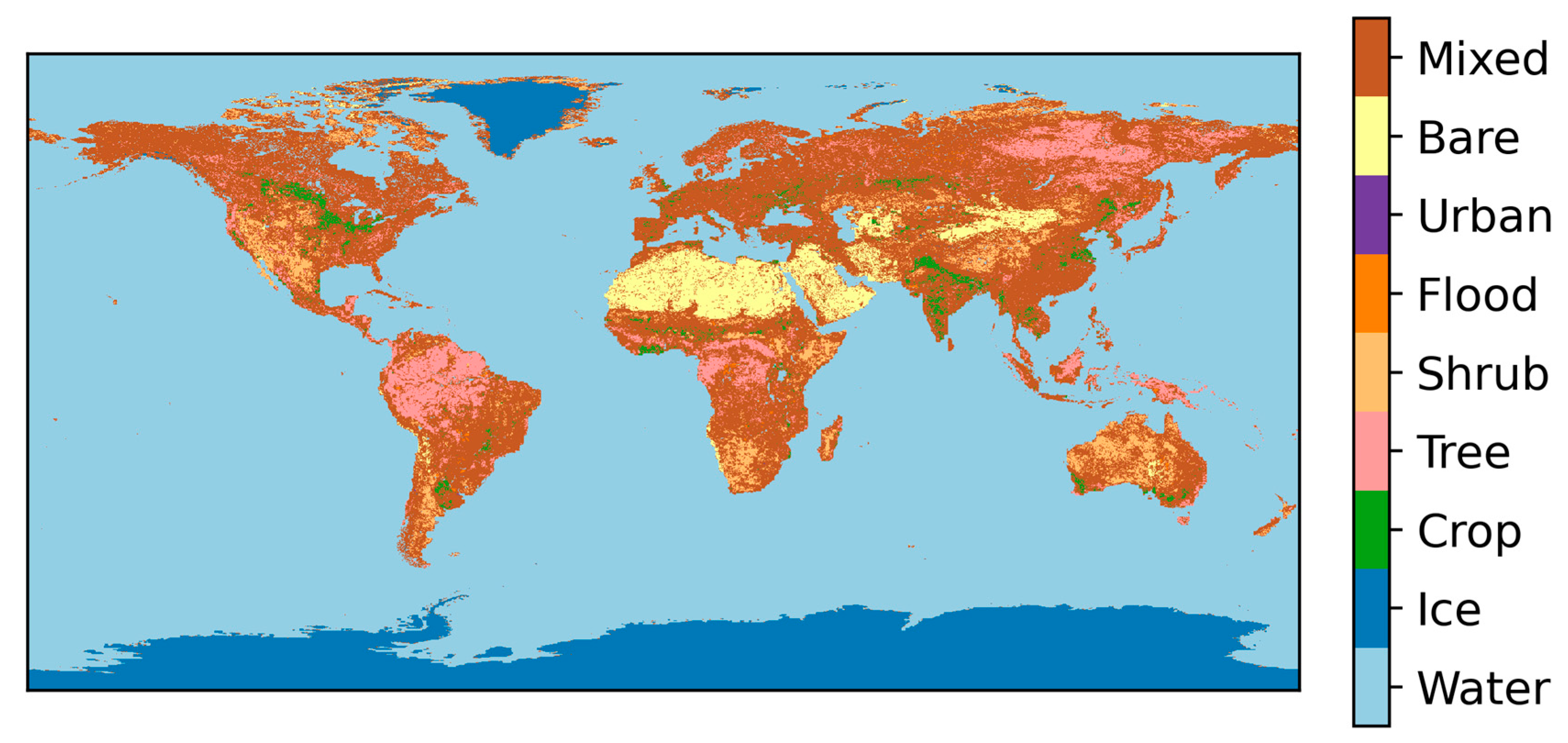
For the purposes of modelling spatial sampling uncertainty, sub-setting the full 42 land cover definitions into eight key biome definitions is sufficient. The dominant land cover class (from the 42 classes) is identified first, at the given resolution. For each grid cell, the percentage coverage of the dominant land cover class is also provided, relative to land cover map at 0.01°. A threshold of ≥95% applied to this to identify those grid cells that are of a ‘single’ biome. These are then grouped together under seven different dominant biome definitions: tree, flood, urban, crop, bare, shrub, and permanent snow and ice. The grouping of these land cover classes into dominant biomes is as defined in ([23], Table 2). The remainder of the grid cells over land, with <95% coverage by a single land cover class, are classified as ‘mixed’. The spatial distribution of these biomes globally at 0.1° resolution is as shown in Figure 2.

2.2. Sampling Uncertainty Derivation

A full derivation of the sampling uncertainty calculation was first published in [17], and we provide here an overview of the methodology as applied to LST data, sufficient to follow the sampling uncertainty modelling presented in this paper. Considering the case where we have a fully clear-sky grid cell with a sample size of $n$ pixels, the LST for the grid cell ($\widehat{{LST}_n}$) is simply the arithmetic mean of the input pixels.

$$\widehat{{LST}_n}={\displaystyle \frac{1}{n}}\sum _{i=1}^n{LST}_i$$

(1)

If we take a subsample of $m$ pixels from within the clear-sky grid cell, the average LST within the subsample is defined over the $m$ pixels.

$$\widehat{{LST}_m}={\displaystyle \frac{1}{m}}\sum _{j=1}^m{LST}_j$$

(2)

The subsampling error $E$ is the difference between $\widehat{{LST}_m}$ and $\widehat{{LST}_n}$, which can be written as

$$E=\left({\displaystyle \frac{1}{m}}-{\displaystyle \frac{1}{n}}\right)\sum _{j=1}^m{LST}_j-{\displaystyle \frac{1}{n}}\sum _{h=1}^{n-m}{LST}_h$$

(3)

where $h$ represents the pixels in sample $n$ that are not included in sample $m$. $E$ is defined here under the assumption of a perfect LST retrieval. In reality, noise in the radiance measured by the MODIS instrument propagates through into the LST retrieval, meaning that we only have an estimate of the sampling uncertainty, $\widehat{E}$. $\widehat{E}$ is related to $E$ as in (4), where $e_E$ is the contribution of the noise to the estimation of $\widehat{E}$.

$$\widehat{E}=E+e_E$$

(4)

The sampling uncertainty ($SU$) is the square root of the variance of $E$ over multiple samples ($K$). Under the assumption that $e_E$ is independent and uncorrelated with $\widehat{E}$, the variance in $E$ can be defined as

$$var(E)=var\left(\widehat{E}\right)-var(e_E)$$

(5)

$$SU={\left[var\left(E\right)\right]}^{1/2}$$

(6)

Using Equation (3), and assuming a per-pixel noise of 0.2 K, we can propagate this through the LST difference calculation to obtain the noise in the calculated difference, ${ϵ}_E$. The per-pixel noise is estimated given knowledge of the noise in each sensor channel used to retrieve LST and the magnitude of this uncertainty when propagated through the retrieval equation.

$${ϵ}_E={\left[{\left({\displaystyle \frac{1}{m}}-{\displaystyle \frac{1}{n}}\right)}^2\sum _{j=1}^m{ϵ}_j^2-{\left({\displaystyle \frac{1}{n}}\right)}^2\sum _{h=1}^{n-m}{ϵ}_h^2\right]}^{1/2}$$

(7)

Substituting (7) into (6) and assuming the variance in $\widehat{E}$ to be an unbiased estimate of the sampling uncertainty, $SU$ is defined as

$$SU={\left[\left({\displaystyle \frac{1}{K-1}}{\sum \left(\widehat{E}-{\displaystyle \frac{1}{K}}\sum _{k=1}^K{\widehat{E}}_k\right)}^2\right)-\left({\displaystyle \frac{1}{K}}\sum _{k=1}^K{ϵ}_{E_k}^2\right)\right]}^{1/2}$$

(8)

2.3. Subsampling Strategy

Spatial sampling uncertainty will always vary as a function of the clear-sky fraction [17]—the fewer observations available, the less likely the subsample is to fully represent the target area under all but the most homogeneous of conditions. Consequently, spatial sampling uncertainty is modelled for each clear-sky percentage represented by adding/removing a single pixel; e.g., for the target resolution of 0.05°, the sample size is 25 pixels giving clear-sky percentage intervals of 4% (1/25 = 0.04). For the target resolution of 0.1°, the clear-sky percentage interval is 1%.

For each subsample size (1–24 pixels in the 0.05° case, 1–99 for the 0.1° case), we apply 500 different, realistic cloud masks to the fully clear-sky sample to give the appropriate subsample size. These realistic cloud masks are identical to those applied in [17] and were extracted by sampling data from the Advanced Along Track Scanning Radiometer (AATSR) that had been masked using the Bayesian cloud detection scheme as part of the ESA SST CCI project [2,17]. Although cloud characteristics can differ between the land and ocean [24], these masks are applicable here as they characterize only the shape of cloud edges as imposed on partially observed grid cells. Realistic cloud masks are used as [17] demonstrated the importance of correctly characterizing the cloud structure in the subsampling.

To make the spatial sampling uncertainty modelling computationally efficient, the clear-sky extracts within each biome classification (see Section 2.1) had to be subsampled. This was achieved by using every $n$th extract, where $n$ was dependent on the total number of extracts for the given biome (there were a greater number of extracts over ice than urban regions, for example, due to the orbit characteristics of the sensor and the land coverage of the given biome). This approach was taken to ensure good representation of data at different latitudes and in different seasons (within the constraints of where different biomes are located geographically).

Table 1. Number of clear-sky data extracts analyzed for each biome and target resolution.

Biome	0.05° Target Resolution	0.1° Target Resolution
Ice	28,349	61,405
Crop	4031	7460
Tree	11,287	20,489
Shrub	18,636	33,570
Flood	18,413	37,750
Urban	5105	7512
Bare	20,654	43,005
Mixed	12,732	23,170

shows the number of extracts used for each target resolution and biome (for which the 500 different cloud masks were then applied at every subsampling resolution).

3. Results

3.1. Comparing the Sampling Uncertainty Model and Current Parameterisation in ESA LST CCI Products

We first calculate a global spatial sampling uncertainty model, with results subdivided by the biome classification (Figure 3a,b). In the case of 100% clear sky, sampling uncertainty is zero. This typically rises as the clear-sky fraction is reduced. At the target resolution of 0.05°, the spatial sampling uncertainty remains < 1 K for all biomes and subsample sizes. The largest sampling uncertainties are seen for mixed pixels (max 0.99 K), which is intuitive as these have the most variable land surface cover within a given grid cell. The lowest sampling uncertainties are seen for ice pixels, reaching a maximum of 0.18 K. As observed from space at a spatial resolution of ~1 km, polar ice is more spatially uniform than other surface types. Cloud detection performance may also be poorer here due to the similarity in the thermal signature of ice and cloud as viewed from space [25,26] (no information from channels at reflectance wavelengths is used in the cloud detection employed when generating these products [27]). The shape of the sampling uncertainty curve is consistent between biomes (although the magnitude varies), with the exception of urban grid cells. Here, sampling uncertainties remain lower for clear-sky percentages between 20 and 60% before rapidly increasing for clear-sky percentages < 20%.

For a target resolution of 0.1°, the shape of the sampling uncertainty curve remains consistent, but the magnitude of the uncertainties is inflated. This differs from the sea surface temperature case, where it was found that the sampling uncertainty model was consistent across the two target resolutions. The ordering of the maximum sampling uncertainty (ice, bare, crop, flood, tree, shrub, mixed) is consistent, except for urban grid cells, which have the largest sampling uncertainty (2.5 K) at this target resolution. At a resolution of ~10 × 10 km, cities may be, on average, more heterogeneous than at ~5 × 5 km, with variability introduced by housing, businesses, parks, shopping centres, and construction work, which would increase sampling uncertainty. These areas can also be quite segregated from one another, so a structured cloud mask imposed on the clear-sky extract may preferentially exclude one element of the city, e.g., a business park, but not others. Larger grid cell sizes also increase the potential for inclusion of non-urban materials at the edges of urban areas, increasing heterogeneity.

The bottom panel of Figure 3 contrasts the results given when applying the equation currently used to calculate sampling uncertainty, ($u_{samp}$, spatial or temporal) in ESA LST CCI products (Equation (9)) [16,28]. In this panel, the mean sampling uncertainty is shown when applying this equation across all extracts and subsample sizes. In Equation (9), $n$ is the total number of pixels in the extract, $n_{cld}$ the number of cloudy pixels, $n_{clr}$ the number of available clear-sky pixels, and ${\sigma }_{n_{clr}}^2$ the variance in the LST over the clear-sky subsample.

$$u_{samp}={\displaystyle \frac{n_{cld}{\sigma }_{n_{clr}}^2}{n-1}}$$

(9)

Figure 3 demonstrates that the utility of a sampling uncertainty calculated in this manner is limited. The shape of the curve is inconsistent with a true sampling uncertainty model—sampling uncertainty increases as the clear-sky percentage reduces to between 20 and 40% and then falls again. This trend towards zero at low clear-sky fractions is due to the dependence of Equation (9) on the LST variance within the clear-sky subsample. For a subsample size of 1, the variance is 0 and thus so too is the sampling uncertainty.

For the first part of the sampling uncertainty curve (40–100% clear sky), the shape of the curve is convex rather than concave, but the absolute values are reasonably consistent with the $SU$ model (Figure 3a,b). Note, however, that in these panels the quantity plotted is the mean sampling uncertainty across all clear-sky extracts, which hides some of the variability in the calculated sampling uncertainty. In some cases, using Equation (9) inflates the sampling uncertainty considerably (>10 K), which can be mitigated to some extent by using a climatology of the LST variance.

3.2. Evaluating Other Dependencies of the Sampling Uncertainty Model

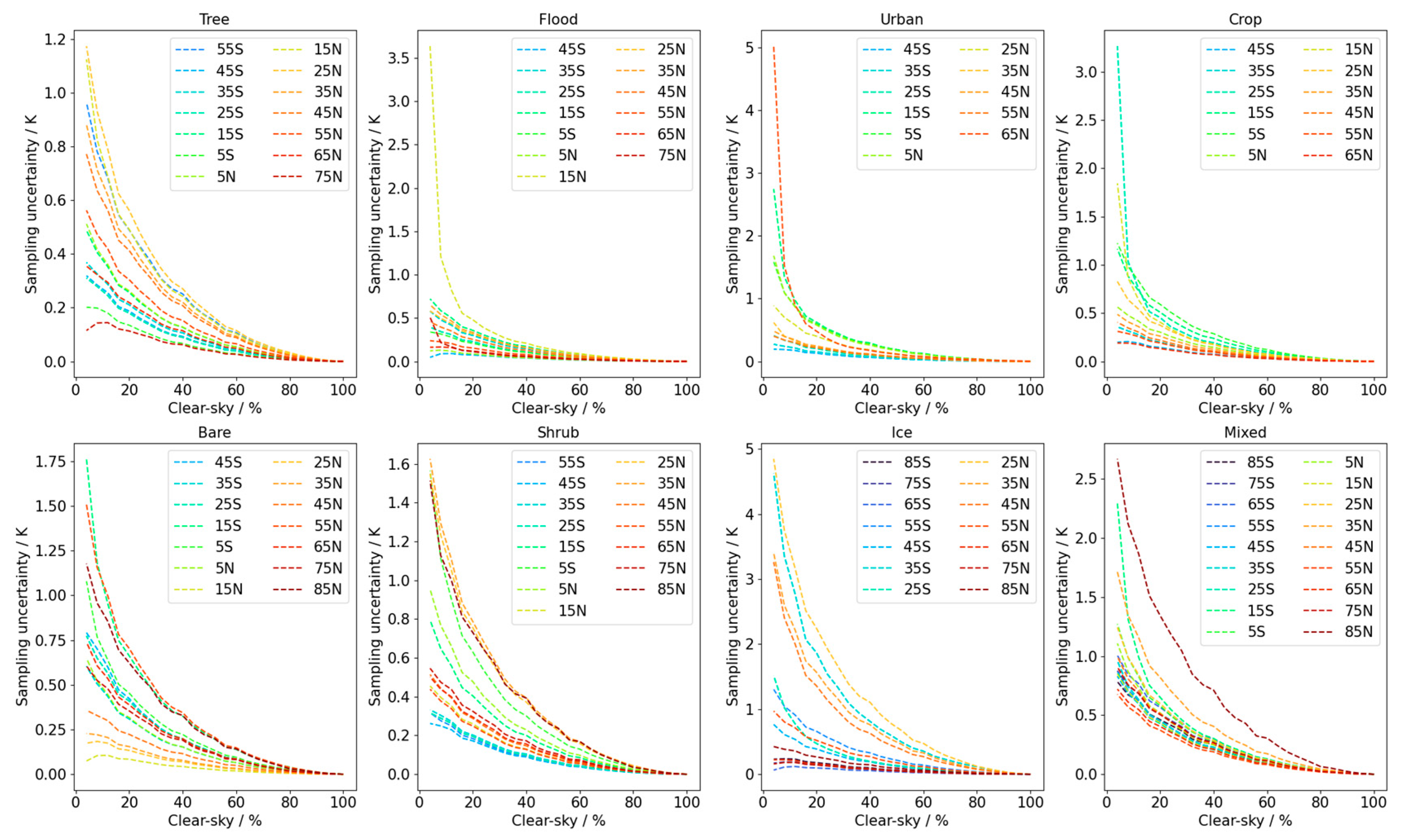
The magnitude of spatial sampling uncertainty is dependent on the degree of heterogeneity in the surface as observed by the satellite sensor. Over land, this may vary as a function of latitude (if the ‘appearance’ of the land cover type varies significantly with climate zone) or as a function of illumination (solar zenith angle). We examine both dependencies here. Figure 4 shows the latitudinal dependency of sampling uncertainty at the target resolution of 0.05°. The extract sampling in this example is such that all latitudes are well sampled, where data exist. Many biomes show considerable variability in spatial sampling uncertainty with latitude, but it is most useful to interpret these results with reference to Figure 3. Where the global sampling uncertainty model lies in the centre of the latitudinal spread of sampling uncertainty, this indicates that latitudinal variability should be considered in any sampling uncertainty model. In other cases, the latitudinal variability of a given biome may be minimal, i.e., ice is predominantly found in polar regions. At a target resolution of 0.05°, the latitudinal variability in spatial sampling uncertainty is most important for the shrub, bare, tree, and mixed biomes. At a target resolution of 0.1°, it is important for all biomes, except ice and bare (not shown).

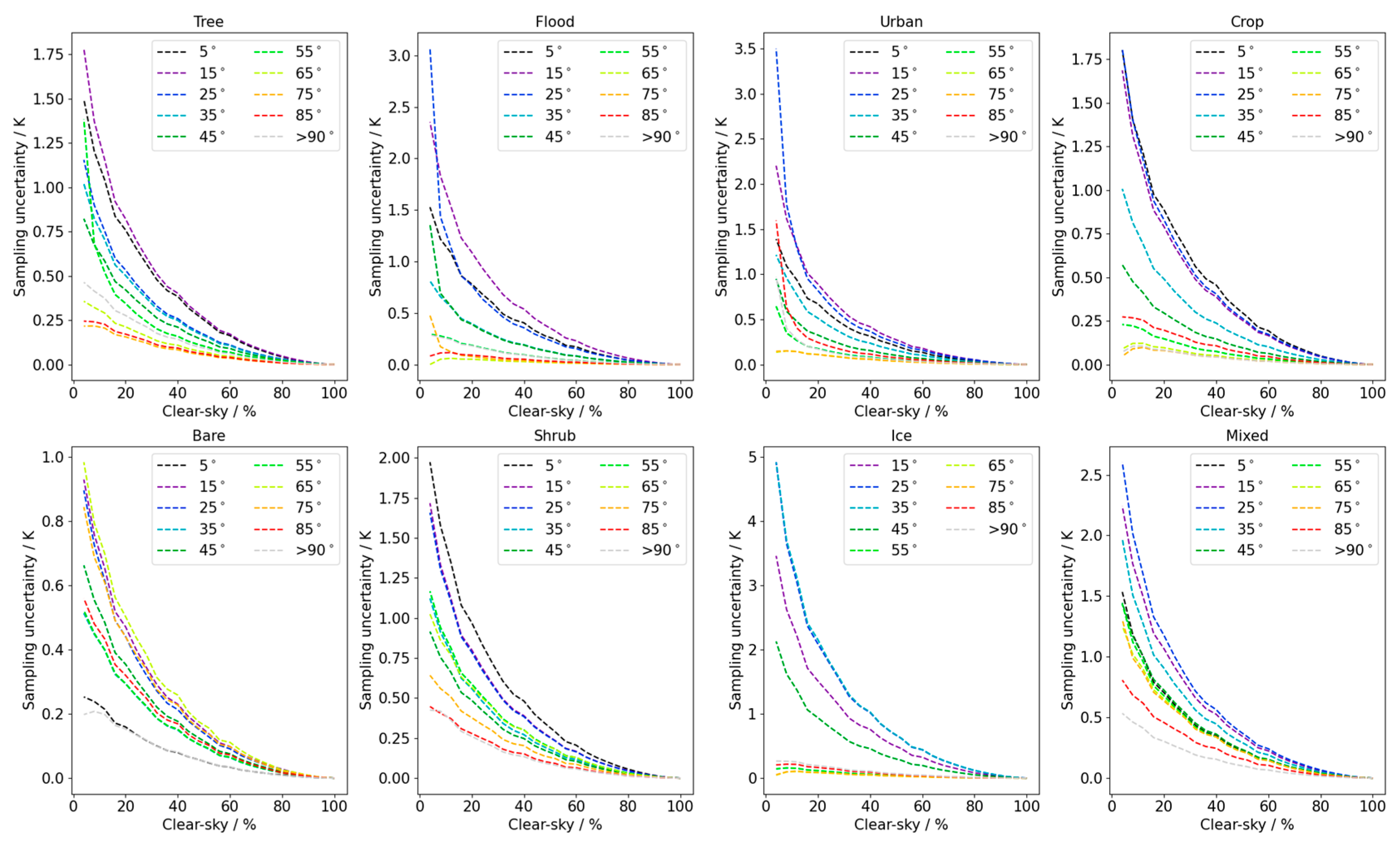
Figure 5 shows the dependence of the sampling uncertainty model on solar zenith angle for the target resolution of 0.05°. For most biomes, the spatial sampling uncertainty is larger when the sun is directly overhead. Under these conditions, the disparity in warming rates between different surface types is most pronounced. At lower illumination angles there is less thermal energy and at night, radiative cooling can reduce temperature discrepancies between different materials. Bare soil is the exception to this pattern, as spatial sampling uncertainty is lowest for solar zenith angles of 0–10° and under nighttime conditions. As bare soil is more uniform at the kilometre scale than many of the other biomes considered here, sampling uncertainty when the sun is not directly overhead may be enhanced by shadowing. Many desert regions have landscapes dominated by sand dunes that will cast shadows under non-nadir solar geometry, increasing the spatial temperature heterogeneity.

At this target resolution, solar zenith angle is an important determiner of the spatial sampling uncertainty magnitude for all biomes except ice. Ice is the exception as most observations are made under night or twilight conditions. The same is true at the 0.1° target resolution, except for ice and bare soil surfaces (not shown).

3.3. Variability Within Mixed Pixels

Mixed pixels are defined as those where <95% of the grid cell is described by a single land cover class (from the original 42, see Section 2.1). Within this definition, there is scope for variability between grid cells, with different numbers of land cover classifications located within a given grid cell and varying percentages of the grid cell represented by the ‘dominant’ land cover class. Note that where multiple land cover classes are present in a given grid cell, the classes themselves are not identified (only the number and dominant class percentage). Therefore, we cannot relate the constituent land cover classes to our seven dominant biome definitions when evaluating these data.

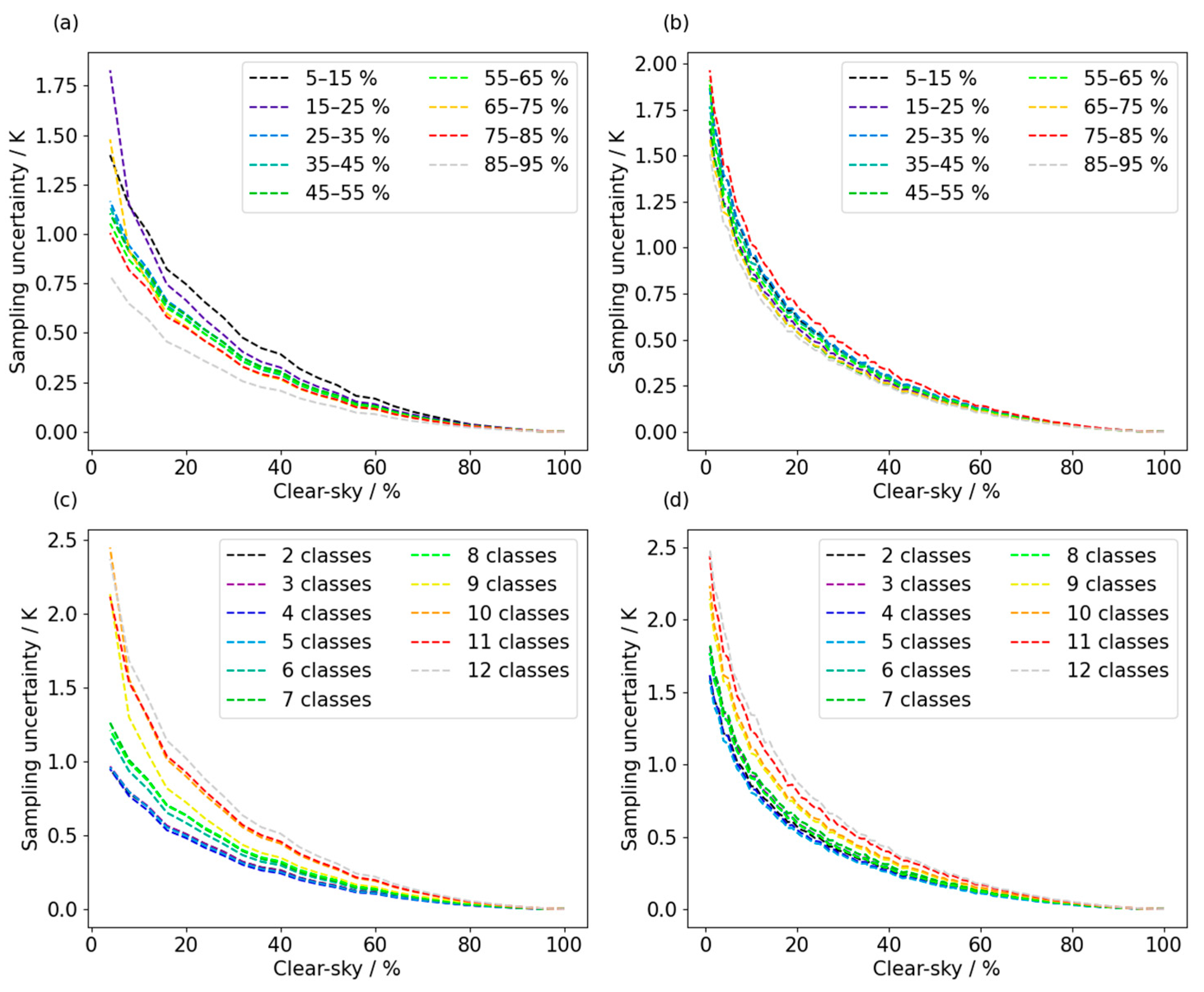
Figure 6 shows the spatial sampling uncertainty dependence on grid cell characteristics for mixed pixels. Considering first the percentage of the grid cell represented by the dominant land cover class (top row), at a target resolution of 0.05°, the magnitude of the spatial sampling uncertainty increases as the percentage decreases. This is intuitive as when the dominant land cover represents a smaller fraction of the grid cell, there must be a larger number of land cover classes present (all with smaller percentages than the dominant one), increasing the surface variability within the grid cell. At a target resolution of 0.1°, the spatial sampling uncertainty magnitude has a much smaller spread at the maximum (~0.5 K, compared to ~1 K at 0.05°) as a function of the dominant land cover class percentage coverage.

Considering the number of different land cover classes present in a grid cell (bottom row), at both target resolutions, the lowest sampling uncertainties are seen when fewer classes are present (with larger sampling uncertainties for large numbers of classes). The spread is again larger at the target resolution of 0.05° (~1.5 K compared with ~0.9 K for the 0.1° resolution).

3.4. Sampling Uncertainty Modelling Strategy for LST Products at 0.05° and 0.1° Resolution

The sampling uncertainty methodology presented in this paper is applicable to all LST datasets generated at the target resolutions of 0.05°and 0.1° (from a starting resolution of 0.01°), providing that the instrument noise propagated through the LST retrieval can be parameterized and removed. It is therefore recommended for implementation in the preparation of uncertainty budgets. With respect to the ESA LST CCI project, Figure 3 clearly demonstrates the need to modify the current sampling uncertainty approach. The results for the 0.05° target resolution are directly applicable to MODIS products that are generated routinely. Data at 0.1° resolution are not routinely provided as part of the product catalogue but can be generated when using the re-gridding tool developed by the project and freely available to data users [29].

Beyond that, this paper has demonstrated that further variability can be captured by including other information about the location and nature of the satellite observation. This paper has demonstrated that latitude, solar zenith angle, and, for mixed pixels only, information on the number of land cover classes in the grid cell can all provide some refinement to the global model. It is recommended that solar zenith angle is used as a main additional discriminator, as this gives the largest differentiation in sampling uncertainty magnitude for the widest range of biomes.

To apply these outcomes in data production, a fourth-order polynomial fit has been made to the data as a function of clear-sky percentage. This better describes the spatial sampling uncertainty curve and the maxima than a lower-order polynomial but can give a slight artificial rise at 99% clear sky for the 0.1° target resolution. This could be omitted in any application of the data by linearly interpolating between the spatial sampling uncertainty at 98% clear sky and 100% clear sky (where spatial sampling uncertainty is zero). The coefficients describing these polynomials are provided in Appendix A of this paper. Polynomial definitions are provided for (1) the global sampling uncertainty model shown in Figure 3 for target resolutions of 0.05° and 0.1° and (2) the sampling uncertainty model for each solar zenith angle band: 10° increments between 0 and 90°, plus nighttime, for each biome (tree, urban, flood, crop, bare, shrub, ice, mixed) and target resolution.

4. Discussion

The results in this paper demonstrate a clear benefit to modelling sampling uncertainty using the framework developed in [17], in comparison with the current approach, which is shown to have limited utility. When applying this approach to LST data, one key difference to the sea surface temperature (SST) case is that the sampling uncertainty model is not consistent across the two target resolutions (0.05° and 0.1°). Consequently, we must consider cases where data are required at resolutions other than the ones evaluated here: (1) re-gridding to resolutions coarser than 0.1° and (2) spatial sampling uncertainty when generating L3 products at 0.01° resolution.

The LST CCI re-gridding tool [29] enables data users to select their own target resolution for re-gridding, based on the gathering of user requirements, which has shown that applications using LST data are extremely diverse, requiring data on different scales and at different resolutions [20]. The spatial sampling uncertainty model from this paper could be implemented for re-gridding requests at 0.05° and 0.1° resolutions, but for other resolutions, current options would be for the tool to revert to the current calculation, or to use the 0.1° model for coarser grids. The former is less than ideal as the approaches have been shown to be inconsistent, and it may not be immediately apparent to users what the differences are. The latter is likely to be an underestimate of the spatial sampling uncertainty at coarser resolutions (on the basis that the sampling uncertainty increases over larger spatial scales as shown by this analysis). The ideal solution would be to extend the analysis presented here to other commonly requested data resolutions and then perhaps limit user choice on re-gridding resolution to several key options, all of which would have an associated spatial sampling uncertainty model.

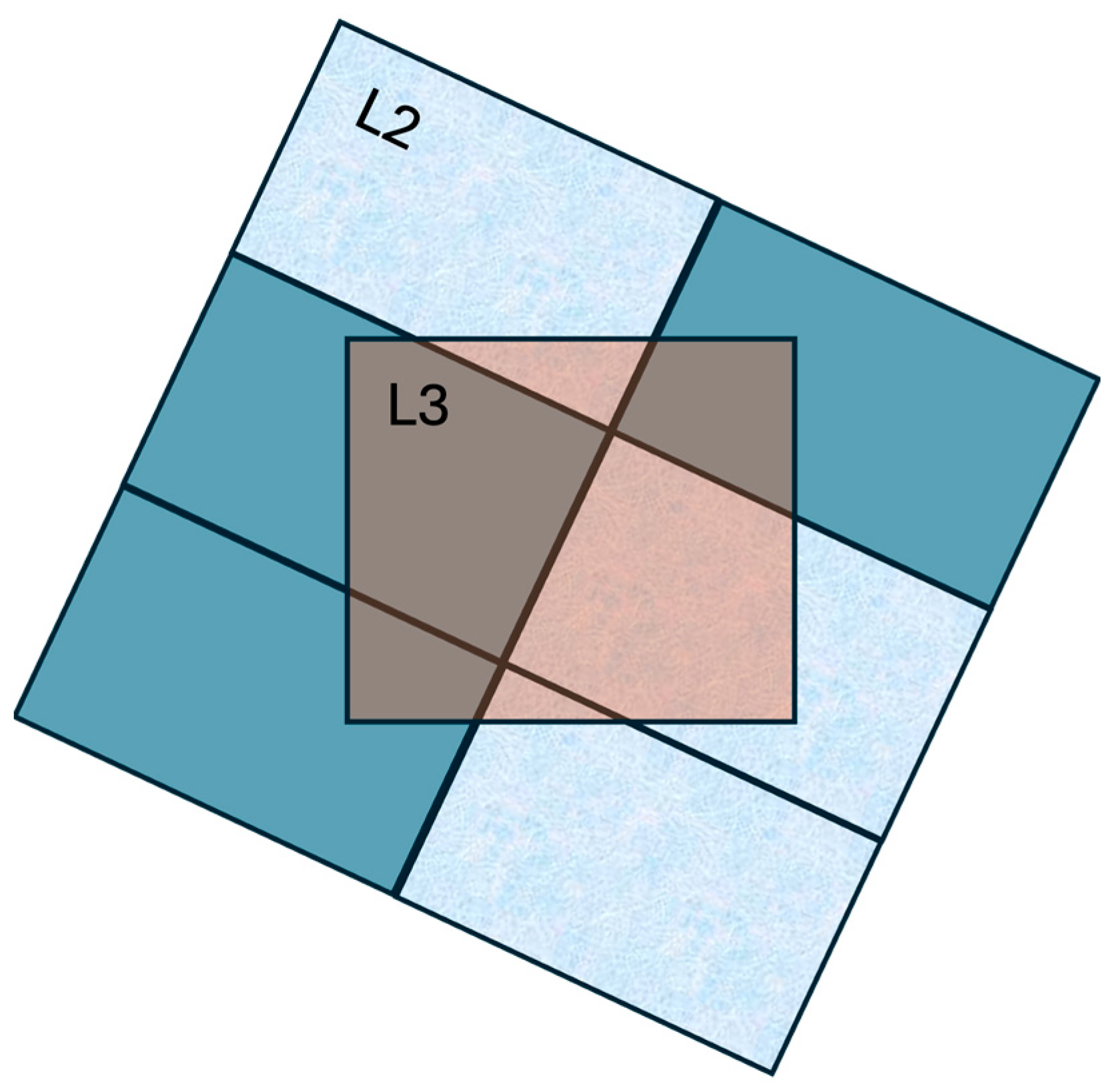
In the LST CCI processing chain, sampling uncertainty is also introduced in the generation of 0.01° Level 3 products (used as the input data for this study). The process of generating regularly gridded observations requires a mapping between the native imagery grid from the satellite sensor and a regular latitude-longitude grid. Although the native resolution of the satellite data (1 km at nadir) is commensurate with the target resolution of 0.01°, the shape and orientation of the image grid can differ significantly from the target grid. In this case, multiple observations may overlap a target grid cell, covering different percentages of the target grid, some of which will be clear sky and some of which will be cloud (Figure 7). There is, therefore, a sampling uncertainty that occurs in this re-gridding step that is currently calculated using Equation (9) but cannot be parameterized using the data presented in this manuscript.

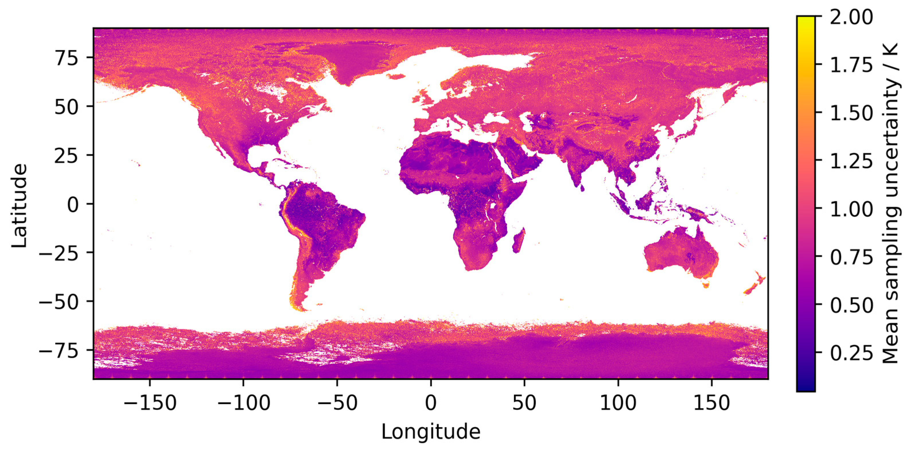
We investigate the degree to which the spatial sampling uncertainty models presented in this manuscript might be applicable to this re-gridding step by evaluating the global mean sampling uncertainty calculated using Equation (9), using all MODIS Terra data (day and night) from 2011, i.e., the same data that form the input for the analysis presented in Section 3. Equation (9) is based on LST variance and therefore the largest sampling uncertainties occur at the boundaries between biomes or along cloud edges where the cloud screening is insufficiently conservative. Elevated mean uncertainties over the year can clearly been seen in transition regions along the edge of the Andes in South America and the boundary between the Sahara and Sahel in Africa (Figure 8).

The global mean uncertainties as a function of biome are shown in

Table 2. Mean sampling uncertainty by biome, estimated using Equation (9), when re-gridding from L2 data on the image grid to L3 at a target resolution of 0.01°.

Biome	Global Mean Sampling Uncertainty/K
Ice	0.95
Crop	0.74
Tree	0.86
Shrub	0.85
Flood	0.92
Urban	0.97
Bare	0.82

. We can compare these to the sampling uncertainty curves in panels (c) and (d) of Figure 3 to determine whether the spatial sampling uncertainty curves calculated here are applicable to this application. The mean values presented in Table 2 are averages across all conditions and in both extremes (completely clear-sky and almost completely cloudy, Equation (9)), we know that this calculation tends to zero. The distribution of clear-sky fraction for each individual L3 0.01° grid cell is unknown, but we would expect the peak to exceed the mean (at ~30% clear-sky fraction using this equation and as shown in Figure 3), given the formulation of the equation.

The maximum peak (applying Equation (9) to the target resolutions of 0.05° and 0.1°) is 0.92 K, for urban pixels at 0.1° resolution. The global mean sampling uncertainty when applying Equation (9) at 0.01° resolution is 0.87 K. Values are more consistent between biomes (min: 0.74 K for cropland; max: 0.97 K for urban areas) than we see at the 0.1° target resolution. This suggests that the dominant source of sampling uncertainty at this resolution is most likely to be cloud boundaries as these do not respect biome divisions (except for broad climatic zone differences). Given the smaller sample size of L2 pixels re-gridded to a L3 0.01° grid cell (typically 6 or fewer) when compared to 25 at a target resolution of 0.05° and 100 at a target resolution of 0.1°, a single unflagged cloudy pixel at a cloud edge has the potential to significantly inflate the ‘LST’ variance at this resolution, thus inflating the mean sampling uncertainty. At the larger spatial resolutions, the effect of one or two misclassified pixels would be more dilute.

Based on this analysis, the best available spatial sampling uncertainty curve from this manuscript, that could be applied to the L2 to L3 re-gridding problem is the global urban curve at 0.1° resolution. The benefits of applying this parameterization at this step would be a better representation of the maximum sampling uncertainties at low clear-sky fractions that cannot be captured by applying Equation (9). The trade-off would be a likely underestimation of the sampling uncertainty at lower clear-sky fractions, given how close the global mean is to the urban curve maximum when applying Equation (9). The better solution would be to use completely clear-sky L2 extracts and the methodology presented in this manuscript to determine a bespoke spatial sampling uncertainty curve for 0.01° L3 data, with full accounting for the fractional representation of the L3 grid cell by each L2 pixel, but this is beyond the scope of this manuscript.

As stated in Section 3.4, these sampling uncertainty methods are also applicable in the calculation of uncertainty budgets for other LST products with an input data resolution of 0.01°/~1 km. The MODIS polynomials presented here could be applied to other polar-orbiting sensors with similar overpass times and spatial resolution. The analysis of a complete year of MODIS Terra data folds in the variability in pixel size from 1 km at nadir to ~4.8 km at the swath edge [30]. The definition of the dominant biomes is broad enough that it should be possible to use the models even if the underlying land cover classification uses a different system. Further investigation is required to see whether the same spatial sampling model is applicable to data from instruments with significantly different equator overpass times, e.g., MODIS Aqua, or coarser native resolution and more extreme viewing angles, e.g., geostationary satellites, where the observation footprint is typically 3–5 km at nadir and viewing zenith angles can reach 60–70° at the disc edge. Even in these cases, there may be some benefit in parameterizing the uncertainty using the polynomials presented here if the alternative is to assign a sampling uncertainty model in which there is less confidence (in terms of both shape and magnitude). The most likely differences between sensors when applying the methodology presented here would be in magnitude, related to the LST variability. In many use cases, uncertainties are used to distinguish those observations that less uncertain from those with a greater uncertainty, for which the shape of the spatial sampling uncertainty curve with respect to clear-sky fraction may be of more importance than small variations in the magnitude.

5. Conclusions

In this manuscript, we develop a spatial sampling uncertainty parameterization for the re-gridding of land surface temperature (LST) data from an original grid at 0.01° resolution to target resolutions of 0.05° and 0.1°. We demonstrate that, to fully capture the variability in the spatial sampling uncertainty, it is appropriate to parameterize this as a function of both the underlying land cover (biome) and the solar zenith angle at the time of the observation. We provide the coefficients for these spatial sampling uncertainty curves, such that any data providers can implement these spatial sampling uncertainty models for products at the given target resolutions.

Both the differences in the magnitude of the spatial sampling uncertainty at different target resolutions and the differences between calculating the spatial sampling uncertainty explicitly (as performed here) and approximating it, highlight the necessity of applying this methodology to data at all resolutions of interest to LST data users. The formulation of the method applied in this manuscript is such that it can be applied to any infrared sensor for which data needs to be coarsened from 0.01° to a target resolution of 0.05° or 0.1°, irrespective of instrument or retrieval, assuming that the noise in the retrieval can be parameterised and removed. Further work is also required to integrate this with a parameterization for temporal sampling uncertainty.

References

1. Global Climate Observing System. The 2022 GCOS Implementation Plan; WMO: Geneva, Switzerland, 2022; p. 98. [Google Scholar]
2. Embury, O.; Merchant, C.J.; Good, S.A.; Rayner, N.A.; Høyer, J.L.; Atkinson, C.; Block, T.; Alerskans, E.; Pearson, K.J.; Worsfold, M.; et al. Satellite-Based Time-Series of Sea-Surface Temperature since 1980 for Climate Applications. Sci. Data 2024, 11, 326. [Google Scholar] [CrossRef]
3. Ghent, D.J.; Corlett, G.K.; Göttsche, F.-M.; Remedios, J.J. Global Land Surface Temperature from the Along-Track Scanning Radiometers. J. Geophys. Res. Atmos. 2017, 122, 12167–12193. [Google Scholar] [CrossRef]
4. Hollmann, R.; Merchant, C.J.; Saunders, R.; Downy, C.; Buchwitz, M.; Cazenave, A.; Chuvieco, E.; Defourny, P.; de Leeuw, G.; Forsberg, R.; et al. The ESA Climate Change Initiative: Satellite Data Records for Essential Climate Variables. Bull. Am. Meteorol. Soc. 2013, 94, 1541–1552. [Google Scholar] [CrossRef]
5. Popp, T.; De Leeuw, G.; Bingen, C.; Brühl, C.; Capelle, V.; Chedin, A.; Clarisse, L.; Dubovik, O.; Grainger, R.; Griesfeller, J.; et al. Development, Production and Evaluation of Aerosol Climate Data Records from European Satellite Observations (Aerosol_cci). Remote Sens. 2016, 8, 421. [Google Scholar] [CrossRef]
6. Devasthale, A.; Karlsson, K.-G. Decadal Stability and Trends in the Global Cloud Amount and Cloud Top Temperature in the Satellite-Based Climate Data Records. Remote Sens. 2023, 15, 3819. [Google Scholar] [CrossRef]
7. Ablain, M.; Legeais, J.F.; Prandi, P.; Marcos, M.; Fenoglio-Marc, L.; Dieng, H.B.; Benveniste, J.; Cazenave, A. Satellite Altimetry-Based Sea Level at Global and Regional Scales. In Integrative Study of the Mean Sea Level and Its Components; Cazenave, A., Champollion, N., Paul, F., Benveniste, J., Eds.; Springer International Publishing: Cham, Switzerland, 2017; pp. 9–33. ISBN 978-3-319-56490-6. [Google Scholar]
8. Zhang, Y.; Pan, M.; Sheffield, J.; Siemann, A.L.; Fisher, C.K.; Liang, M.; Beck, H.E.; Wanders, N.; MacCracken, R.F.; Houser, P.R.; et al. A Climate Data Record (CDR) for the Global Terrestrial Water Budget: 1984–2010. Hydrol. Earth Syst. Sci. 2018, 22, 241–263. [Google Scholar] [CrossRef]
9. Preimesberger, W.; Scanlon, T.; Su, C.-H.; Gruber, A.; Dorigo, W. Homogenization of Structural Breaks in the Global ESA CCI Soil Moisture Multisatellite Climate Data Record. IEEE Trans. Geosci. Remote Sens. 2021, 59, 2845–2862. [Google Scholar] [CrossRef]
10. Merchant, C.J.; Paul, F.; Popp, T.; Ablain, M.; Bontemps, S.; Defourny, P.; Hollmann, R.; Lavergne, T.; Laeng, A.; de Leeuw, G.; et al. Uncertainty Information in Climate Data Records from Earth Observation. Earth Syst. Sci. Data 2017, 9, 511–527. [Google Scholar] [CrossRef]
11. Woolliams, E.R.; Mittaz, J.P.; Merchant, C.J.; Hunt, S.E.; Harris, P.M. Applying Metrological Techniques to Satellite Fundamental Climate Data Records. J. Phys. Conf. Ser. 2018, 972, 012003. [Google Scholar] [CrossRef]
12. Mittaz, J.; Merchant, C.J.; Woolliams, E.R. Applying Principles of Metrology to Historical Earth Observations from Satellites. Metrologia 2019, 56, 032002. [Google Scholar] [CrossRef]
13. Merchant, C.; Holl, G.; Mittaz, J.; Woolliams, E. Radiance Uncertainty Characterisation to Facilitate Climate Data Record Creation. Remote Sens. 2019, 11, 474. [Google Scholar] [CrossRef]
14. Bulgin, C.E.; Embury, O.; Corlett, G.; Merchant, C.J. Independent Uncertainty Estimates for Coefficient Based Sea Surface Temperature Retrieval from the Along-Track Scanning Radiometer Instruments. Remote Sens. Environ. 2016, 178, 213–222. [Google Scholar] [CrossRef]
15. Ablain, M.; Meyssignac, B.; Zawadzki, L.; Jugier, R.; Ribes, A.; Spada, G.; Benveniste, J.; Cazenave, A.; Picot, N. Uncertainty in Satellite Estimates of Global Mean Sea-Level Changes, Trend and Acceleration. Earth Syst. Sci. Data 2019, 11, 1189–1202. [Google Scholar] [CrossRef]
16. Ghent, D.; Veal, K.; Trent, T.; Dodd, E.; Sembhi, H.; Remedios, J. A New Approach to Defining Uncertainties for MODIS Land Surface Temperature. Remote Sens. 2019, 11, 1021. [Google Scholar] [CrossRef]
17. Bulgin, C.E.; Embury, O.; Merchant, C.J. Sampling Uncertainty in Gridded Sea Surface Temperature Products and Advanced Very High Resolution Radiometer (AVHRR) Global Area Coverage (GAC) Data. Remote Sens. Environ. 2016, 177, 287–294. [Google Scholar] [CrossRef]
18. Glissenaar, I.; Boersma, K.F.; Anglou, I.; Rijsdijk, P.; Verhoelst, T.; Compernolle, S.; Pinardi, G.; Lambert, J.-C.; Van Roozendael, M.; Eskes, H. TROPOMI Level 3 Tropospheric NO2 Dataset with Advanced Uncertainty Analysis from the ESA CCI+ ECV Precursor Project. Earth Syst. Sci. Data 2025, 17, 4627–4650. [Google Scholar] [CrossRef]
19. Merchant, C.J.; Harris, A.R.; Maturi, E.; Maccallum, S. Probabilistic Physically Based Cloud Screening of Satellite Infrared Imagery for Operational Sea Surface Temperature Retrieval. Q. J. R. Meteorol. Soc. 2005, 131, 2735–2755. [Google Scholar] [CrossRef]
20. Aldred, F.; Good, E.; Bulgin, C.; Rayner, N. User Requirements Document. 2023. Available online: https://admin.climate.esa.int/documents/2199/LST-CCI-D1.1-URD_-_i3r0_-_User_Requirement_Document.pdf (accessed on 1 August 2025).
21. Bontemps, S.; Boettcher, M.; Brockmann, C.; Kirches, G.; Lamarche, C.; Radoux, J.; Santoro, M.; Vanbogaert, E.; Wegmüller, U.; Herold, M.; et al. Multi-Year Global Land Cover Mapping at 300 m and Characterization for Climate Modelling: Achievements of the Land Cover Component of the ESA Climate Change Initiative. Int. Arch. Photogramm. Remote Sens. Spat. Inf. Sci. 2015, XL-7-W3, 323–328. [Google Scholar] [CrossRef]
22. Kirches, G.; Brockmann, C.; Boettcher, M.; Peters, M.; Bontemps, S.; Lanarche, C.; Schlerf, M.; Santoro, M. Land Cover CCI Product User Guide Version 2. 2014. Available online: https://maps.elie.ucl.ac.be/CCI/viewer/download/ESACCI-LC-Ph2-PUGv2_2.0.pdf (accessed on 7 October 2025).
23. Bulgin, C.E.; Embury, O.; Maidment, R.I.; Merchant, C.J. Bayesian Cloud Detection over Land for Climate Data Records. Remote Sens. 2022, 14, 2231. [Google Scholar] [CrossRef]
24. Chi, Y.; Zhao, C.; Yang, Y.; Zhao, X.; Yang, J. Global Characteristics of Cloud Macro-Physical Properties from Active Satellite Remote Sensing. Atmos. Res. 2024, 302, 107316. [Google Scholar] [CrossRef]
25. Liu, Y.; Ackerman, S.A.; Maddux, B.C.; Key, J.R.; Frey, R.A. Errors in Cloud Detection over the Arctic Using a Satellite Imager and Implications for Observing Feedback Mechanisms. J. Clim. 2010, 23, 1894–1907. [Google Scholar] [CrossRef]
26. Hall, D.K.; Key, J.R.; Casey, K.A.; Riggs, G.A.; Cavalieri, D.J. Sea Ice Surface Temperature Product from MODIS. IEEE Trans. Geosci. Remote Sens. 2004, 42, 1076–1087. [Google Scholar] [CrossRef]
27. Bulgin, C.E.; Sembhi, H.; Ghent, D.; Remedios, J.J.; Merchant, C.J. Cloud-Clearing Techniques over Land for Land-Surface Temperature Retrieval from the Advanced Along-Track Scanning Radiometer. Int. J. Remote Sens. 2014, 35, 3594–3615. [Google Scholar] [CrossRef]
28. Bulgin, C.; Ermida, S.; Jimenez, C.; Veal, K. End-To-End ECV Uncertainty Budget. 2023. Available online: https://admin.climate.esa.int/media/documents/LST-CCI-D2.3-E3UB_-_i3r0_-_End-to-End_ECV_Uncertainty_Budget.pdf (accessed on 1 August 2025).
29. LST CCI. Re-Gridding and Sub-Setting User Manual. 2023. Available online: https://climate.esa.int/en/projects/land-surface-temperature/tool/ (accessed on 1 August 2025).
30. Minnett, P.J.; Alvera-Azcárate, A.; Chin, T.M.; Corlett, G.K.; Gentemann, C.L.; Karagali, I.; Li, X.; Marsouin, A.; Marullo, S.; Maturi, E.; et al. Half a Century of Satellite Remote Sensing of Sea-Surface Temperature. Remote Sens. Environ. 2019, 233, 111366. [Google Scholar] [CrossRef]
Figure 1. Sampling density of clear-sky extracts for each 10-degree tile at 0.1° resolution as a function of season: (a) DJF, (b) MAM, (c) JJA, and (d) SON. Clear-sky extracts are taken from both daytime and nighttime retrievals.
Remotesensing 17 03435 g001
Figure 2. Spatial distribution of the seven dominant biomes used in this study at the target resolution of 0.1°—ice, crop, tree, shrub, flood, urban, and bare—along with ‘mixed’ grid cell locations. Water grid cells are shown for completeness but are not used in this study.
Remotesensing 17 03435 g002
Figure 3. Global spatial sampling uncertainty as a function of biome classification for a target resolution of (a) 0.05° and (b) 0.1°. Dashed lines show the calculated sampling uncertainty and solid lines a fit to the sampling uncertainty curve using a 4th-order polynomial. Panels (c,d) show the average sampling uncertainty for a given clear-sky percentage, when calculated by applying the sampling uncertainty equation currently used for ESA LST CCI products [16,28]. Note that the y-axis ranges differ across the four subplots due the difference in resolutions and methodology.
Remotesensing 17 03435 g003
Figure 4. Latitudinal dependence of sampling uncertainty within each biome classification (top row: flood, urban, shrub, and crop; bottom row: bare, tree, ice and mixed). Southern Hemisphere latitudes are shown in blue and Northern Hemisphere latitudes in red. Legend labels indicate the midpoint of each 10° latitude band represented for a given biome. Note that not all biomes are found at all latitudes.
Remotesensing 17 03435 g004
Figure 5. Solar zenith angle dependence of sampling uncertainty within each biome classification (top row: flood, urban, shrub, and crop; bottom row: bare, tree, ice and mixed). Legend labels indicate the midpoint of each 10° solar zenith angle band represented for a given biome. Note, not all biomes are observed by MODIS Terra under all solar zenith angles.
Remotesensing 17 03435 g005
Figure 6. Sampling uncertainty dependence for mixed pixels on percentage of the grid cell represented by the dominant land cover class (top) and the number of land cover classes found in the grid cell (bottom). Results for a target resolution of 0.05° are shown on the left (panels (a,c)) and for 0.1° on the right (panels (b,d)).
Remotesensing 17 03435 g006
Figure 7. Illustration of the spatial sampling uncertainty when re-gridding L2 satellite observations (blue pixels) on the satellite image grid to a L3 observation (red pixel) on a regular latitude/longitude grid. At the satellite nadir, the L2 pixels have a similar sized footprint to the L3 target resolution of 0.01°, but the orientation of the image grid relative to the L3 pixel can result in an overlap with several pixels. These pixels comprise different percentages of the target grid cell with some cloudy (light blue, textured) and some clear sky (mid blue, plain).
Remotesensing 17 03435 g007
Figure 8. Global mean sampling uncertainty (day and nighttime data combined) for all MODIS Terra data in 2011, re-gridded from the L2 image grid to a L3 product at 0.01° resolution.
Remotesensing 17 03435 g008