Article

Global 0.1-Degree Monthly Mean Hourly Total Canopy Solar-Induced Chlorophyll Fluorescence Dataset Derived from Random Forest

1
School of Geographical Sciences, Nanjing University of Information Science and Technology, Nanjing 210044, China
2
International Institute for Earth System Sciences, Jiangsu Center for Collaborative Innovation in Geographical Information Resource Development and Application, Nanjing University, Nanjing 210023, China
3
Jiangsu Provincial Key Laboratory of Geographic Information Science and Technology, Key Laboratory for Land Satellite Remote Sensing Applications of Ministry of Natural Resources, School of Geography and Ocean Science, Nanjing University, Nanjing 210023, China
4
International Joint Carbon Neutrality Laboratory, Nanjing University, Nanjing 210023, China
*
Author to whom correspondence should be addressed.
Remote Sens. 2025, 17(20), 3429; https://doi.org/10.3390/rs17203429
Submission received: 28 August 2025 / Revised: 11 October 2025 / Accepted: 13 October 2025 / Published: 14 October 2025

Abstract

Highlights

What are the main findings?
  • We have successfully produced a global monthly mean hourly SIF dataset (SIFtotal_01) with a resolution of 0.1° for the years 2000 to 2022.
What is the implication of the main finding?
  • SIFtotal_01 bridges a critical gap between ground-based and spaceborne SIF observations, offering valuable insights for research on ecosystem productivity, climate–carbon feedbacks, and vegetation stress.

Abstract

Photosynthesis drives terrestrial carbon uptake, yet its diurnal dynamics remain poorly resolved due to the sparse availability of flux towers and the coarse spatial resolution of current satellite observations. Solar-induced chlorophyll fluorescence (SIF) provides a direct proxy of carbon uptake, but the existing global monthly mean diurnal total canopy SIF product is limited to 0.5° resolution. We developed a random forest-based downscaling framework to generate a global monthly mean hourly SIF dataset (SIFtotal_01) at 0.1° resolution for 2000–2022. When validated against eddy-covariance-based gross primary productivity (GPP) data, SIFtotal_01 showed a strong correlation (R2 = 0.81) and reduced root mean square error when compared with SIFtotal (2.89→2.8 mW m−2 nm−1), providing notable gains in broadleaved forests (R2: 0.80→0.88 with a root mean square error of 2.32→1.81 mW m−2 nm−1). The SIFtotal_01 dataset revealed a distinct double-peak in the SIFtotal_01–GPP slope, reflecting widespread afternoon depression of photosynthesis, with normalized slopes declining from 1.03 in the morning to 0.98 in the afternoon. Soil moisture modulated this depression pattern, as the afternoon–morning SIFtotal_01 difference increased from 0.02 to 0.10 mW m−2 nm−1 across dry to wet years. Under water stress, SIF yield was more sensitive than absorbed photosynthetic active radiation (APAR), with a doubling of the afternoon–morning SIF yield difference (0.5→1.1 10−3 nm−1), while the afternoon–morning APAR difference showed a smaller change (−300→−180 kJ m−2). This study improves the potential for bridging observational gaps and constraining models offer valuable insights for fundamental and applied research in the analysis of ecosystem productivity, climate-carbon feedbacks, and vegetation stress.

1. Introduction

Photosynthesis, measured as gross primary production (GPP), acts as the largest natural sink of atmospheric carbon dioxide (CO2) and is vital for regulating the global carbon cycle and climate [1,2]. A comprehension of the spatio-temporal dynamics of GPP, particularly the diurnal variability of GPP, is fundamental to predicting the responses of ecosystems to environmental change. [3,4]. The diurnal variations in GPP have been primarily monitored by eddy covariance (EC) flux towers, which provide direct observations of ecosystem CO2 exchange in an ecosystem [5]. However, the sparse and uneven distribution of EC towers limits regional and global representation, while satellite-based remote sensing (RS) offers continuous, large-scale assessments of GPP [6]. Nevertheless, RS-based investigations of the diurnal dynamics of GPP remain relatively limited.
Several studies have used satellite RS data to analyze the diurnal dynamics of GPP at regional to global scales. The well-known FLUXCOM dataset and its newest version, FLUXCOM-X, combine data-driven models with measurements of local EC flux, RS-derived surface reflectance, and auxiliary meteorological data to produce GPP products at sub-daily temporal resolutions [7,8]. However, these sub-daily GPP datasets suffer from errors in both their spatio-temporal dynamics, especially in regions with sparse EC measurements [7]. In addition to these data-driven approaches, geostationary satellites, such as GEO-KOMPASAT-2A, Geostationary Operational Environmental Satellite-R, and Fengyun-4, are being used to monitor regional GPP at minute-level temporal resolutions. Benefiting from having the enhanced spectral capability, they provide high-frequency observations that enable the detailed characterization of diurnal cycles of vegetation activity [9,10,11,12]. Nevertheless, the inherent spatial coverage of geostationary satellite products is confined to specific hemispheres, precluding truly global observation, while the pronounced diurnal variations in sun-sensor geometry introduce significant angular effects that complicate the retrieval and interpretation of solar-induced chlorophyll fluorescence (SIF) data [4]. These constraints collectively hinder their applicability for conducting consistent and large-scale assessments of the diurnal dynamics of GPP [13]. Compared with these two approaches, satellite retrievals of SIF enable a more direct tracking of the diurnal variability of GPP at a global scale [14].
Solar-induced chlorophyll fluorescence, caused by the excitation of chlorophyll molecules by photosynthetically active radiation (PAR), has emerged as a powerful RS signal that directly reflects the photosynthetic activity of vegetation [15,16]. Unlike reflectance-based vegetation indices, SIF is linked to the photosynthetic process through a mechanistic connection, because fluorescence and photochemistry are closely coupled under moderate light conditions [17,18]. Over the last decade, satellite-derived SIF products, such as SIF* [19], RSIF [20], CSIF [21], GOSIF [22], SIFoco2_005 [23], SIF005 [24], and diurnal SIFtotal [14], have been successfully used to track seasonal and interannual variations in GPP across different ecosystems and climatic regions, demonstrating the capability of the products for use in monitoring vegetation productivity across regional to global scales [25,26]. However, most spaceborne SIF products did not correct for sun-sensor geometry effects, and they are retrieved from sun-synchronous platforms, such as the Global Ozone Monitoring Experiment-2 (GOME-2) and the Orbiting the Carbon Observatory-2 (OCO-2) satellites, which provide observations only at fixed local times (i.e., specific overpass times). This temporal limitation constrains their ability to capture sub-daily variations in GPP, making them particularly less useful in documenting diurnal physiological processes that are crucial for understanding interactions between the ecosystem and atmosphere [27].
Recently, the OCO-3 mission on the International Space Station has enabled measurements at multiple times in one day, providing new opportunities to investigate the diurnal variability in SIF [28,29]. For example, Zhang et al. [30] used OCO-3 SIF data to monitor the progression of the physiological response of plants to drought during 2020 in the southwestern US, revealing the existence of an afternoon depression in photosynthesis as an indicator of plant stress. Further, some studies have produced sub-daily SIF products at a regional scale to capture the diurnal dynamics of SIF [31,32]. However, solar geometry, ecosystem type, and canopy structure significantly affect SIF retrieval and the SIF–GPP relationship [33]. To mitigate this effect, the concept of tracking total canopy SIF emission (SIFtotal) has been developed as a geometry-normalized metric that more robustly reflects canopy photosynthetic activity [14]. Despite these advances, the retrieval of sub-daily SIF at a high spatial resolution is limited by OCO-3′s swath width of approximately 10 km. This issue is also compounded by the dependence of SIF magnitude on sun-sensor geometry, which is a function of the observation time [34,35]. As a result, current sub-daily SIFtotal products are provided at a relatively coarse spatial resolution of 0.5°, which limits their applications in regional studies of the carbon cycle and in ecosystem monitoring.
In this study, we developed a random forest-based downscaling framework to enhance the spatial resolution of SIFtotal from 0.5° to 0.1° (SIFtotal_01). We evaluated SIFtotal_01 against eddy covariance GPP observations and compared it with another state-of-the-art satellite SIF dataset to assess its reliability. Finally, we analyzed the diurnal patterns of SIFtotal_01, highlighting its ability to capture physiological processes, such as the afternoon depression of photosynthesis. Our results provide a new high-resolution sub-daily SIF dataset and demonstrate its potential for improving the large-scale monitoring of terrestrial carbon dynamics.

2. Materials and Methods

2.1. Data

A comprehensive summary of all of the datasets used in this study, including their detailed purposes, is provided in Table A1 in Appendix A.1.

2.1.1. The Diurnal Total Canopy SIF Dataset (SIFtotal)

The SIFtotal dataset is a spatiotemporally continuous dataset of monthly mean diurnal values (06:00–18:00 local time) under clear-sky conditions from 2000 to 2022, with a spatial resolution of 0.5° and units of mW m−2 nm−1. This dataset was developed from nadir-viewing SIF retrievals (SIFnadir) that represent instantaneous SIF (SIFinstant) emissions observed at the satellite overpass time from the OCO-3 mission [14]. The SIFnadir measurements are affected by solar zenith angle, sensor viewing geometry, and canopy structure, which limits their direct use as a proxy of canopy-level photosynthesis. To minimize these angular effects, SIFnadir was converted to the total canopy fluorescence emission using a radiative transfer approach [14]. Then, SIFtotal data were generated using an artificial neural network. The artificial neural network’s response variable was the total canopy fluorescence emissions under clear sky conditions from OCO-3, and its predictor variables included the clear-sky absorbed photosynthetic active radiation (APAR), air temperature (Tair), vapor pressure deficit (VPD), soil moisture (SM), and solar zenith angle [14]. The SIFtotal dataset was acquired from https://doi.org/10.12199/nesdc.ecodb.rs.2024.029 (accessed on 18 July 2025).

2.1.2. Diurnal SIF Dataset Produced by Zhao (SIFz)

To compare with our downscaled dataset, SIFtotal_01, an hourly SIFinstant dataset for mainland China during June–August of 2019–2022 (SIFz) was used. The SIFz dataset was downscaled from OCO-3 SIFnadir retrievals using the eXtreme Gradient Boosting model combined with auxiliary data, such as Tair, VPD, surface solar radiation downward (SRdown), SM, land cover, leaf area index (LAI), and near-infrared reflectance of vegetation (NIRv) [32]. For comparison with our SIFtotal_01, we aggregated SIFz from the hourly scale to monthly mean diurnal data.

2.1.3. GPP Dataset

Two types of GPP datasets (FLUXNET2015 and data from the Haibei steppe EC flux station) were used to compare with our SIFtotal_01 dataset [36]. Since the spatial resolution of the SIFtotal_01 dataset was 0.1°, we needed to carefully consider the representativeness of flux footprints when selecting flux observations [37]. We characterized the growth conditions around flux tower sites using the homogeneity of the normalized difference vegetation index (NDVI) [21]. The second criterion of footprint representation was that the land cover at a flux site was required to account for more than 60% of the land cover within the 0.1° grid. Finally, we found that, among the 166 sites in the FLUXNET2015 dataset, only 19 sites were representative of their corresponding 0.1° grid (Figure 1). Using the same approach, we examined the ChinaFLUX data and found that only the Haibei steppe EC flux site met the criterion of footprint representation during 2019–2020. The temporal resolution of all of the EC flux GPP data is half-hourly. To enable a comparison with hourly SIF data, we aggregated the half-hourly GPP data into hourly averages.

2.1.4. Auxiliary Dataset

The auxiliary databases mainly included the fifth generation of the European reanalysis (ERA5-land) dataset with a spatial resolution of 0.1° [38], and products of the moderate-resolution imaging spectroradiometer (MODIS) version 6.1. The hourly ERA5-Land dataset was obtained from https://doi.org/10.24381/cds.e2161bac (accessed on 27 August 2025). In the ERA5-Land dataset, we selected SRdown, Tair, dew point temperature (Tdew), and volumetric soil water (i.e., soil moisture, SM) at four layers. In addition, SRdown provided an accumulated value, which needed to be decomposed into hourly increments before use. Before use, SRdown needed to be interpolated for each 0.1 degree of longitude, while Tdew was used together with Tair to calculate VPD according to the August–Roche–Magnus formula [39]. The mean values of the four-layer SM (SMmean) were also used to predict SIFtotal_01. The hourly ERA5-Land data were provided in Coordinated Universal Time, which needed to be converted to local solar time based on longitude before use. We used NIRv, enhanced vegetation index (EVI), NDVI, LAI, the fraction of absorbed photosynthetic active radiation (FPAR), and land cover from the MODIS products. Monthly NDVI and EVI with 1 km spatial resolution were directly acquired from https://doi.org/10.5067/MODIS/MOD13A3.061 [40] (accessed on 18 July 2025). The method of Badgley et al. [41] was used to calculate the NIRv. Data with 4-day temporal resolution and 500 m spatial resolution were obtained to acquire LAI and FPAR information from https://doi.org/10.5067/MODIS/MCD15A3H.061 (accessed on 18 July 2025) [42], and aggregated from the original 4-day data to monthly values by averaging. The processing of using the five indices involved a strict quality filtering step followed by spatial aggregation. First, only pixels identified as having the highest possible data quality—corresponding to a value of 0 in the primary quality control flags of each MODIS product—were retained. Subsequently, these quality-screened pixels were upscaled to 0.1° and 0.5° grids using an averaging method. The 500 m spatial resolution land cover data were obtained from https://doi.org/10.5067/MODIS/MCD12Q1.061 (accessed on 18 July 2025) [43]. Land cover data were primarily used to screen the data from flux tower sites. For the 0.1° grid, the percentage of each land cover type was calculated. When comparing the relationship between SIFtotal_01 and GPP across different land cover types, due to the limited number of sites for certain land cover types (e.g., only one EC flux site was evergreen broadleaved forests (EBF)), we merged sites with similar land cover types. For example, the EBF and deciduous broadleaved forests (DBF) were combined. Grasslands (GRA) and open shrublands (OSH) were also merged with each other. Woody Savannas (WSA) and savannas (SAV) were combined. In addition, longitude, latitude, month, and hour were included as predictor variables to predict SIFtotal_01.

2.2. Methods

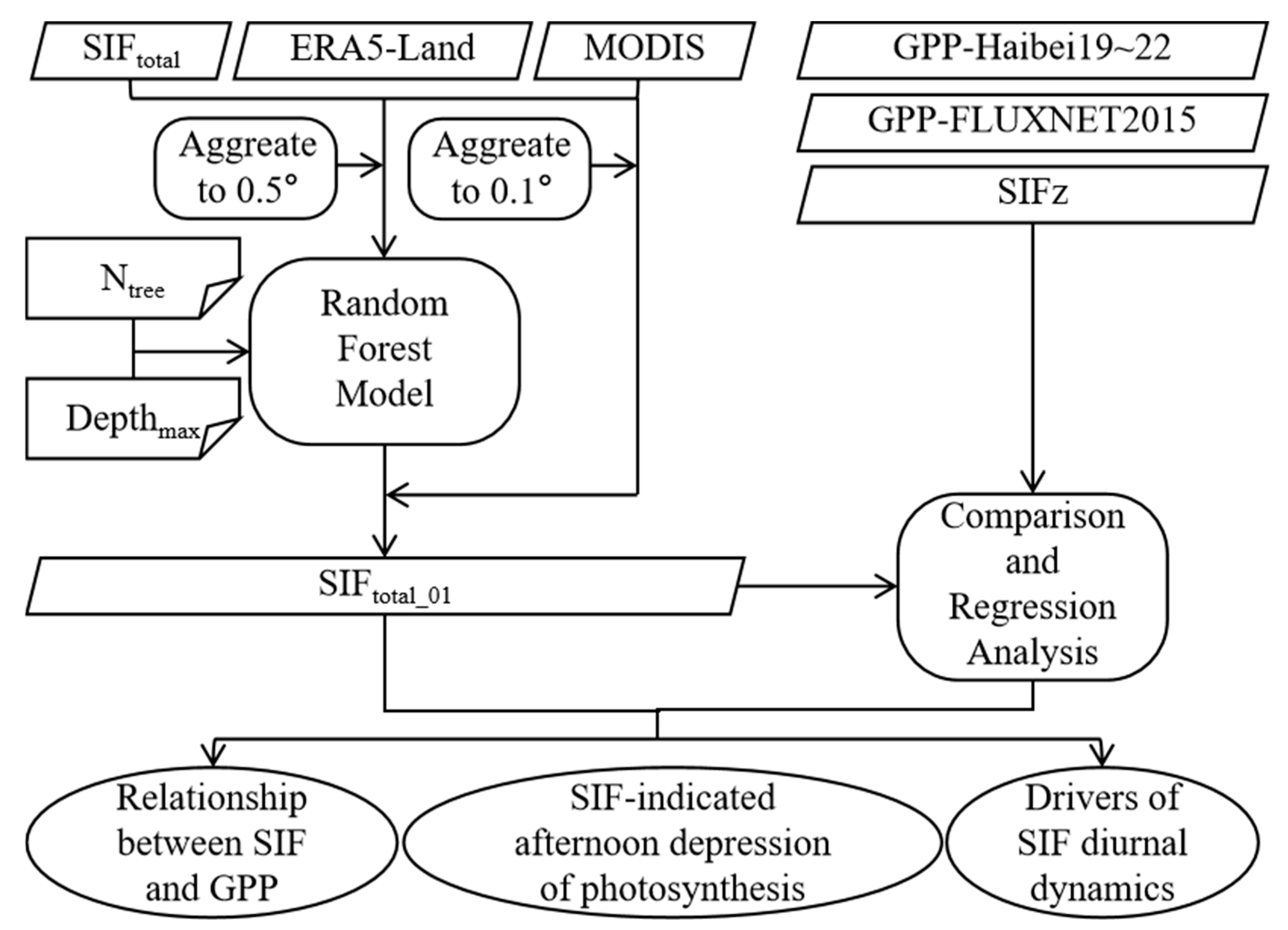
The overall workflow of this study, encompassing data processing, model development, and analysis, is summarized in Figure A1 of the Appendix A.

2.2.1. Model Description

Random Forest (RF) is an ensemble learning method based on the aggregation of multiple decision trees [44]. When using RF, the final prediction is obtained by averaging the outputs of all of the individual trees in the case of regression. In this study, RF was employed to model SIFtotal using 17 predictors at the spatial resolution of 0.5 degree, including ERA5-land data (SRdown, Tair, SM in four layers, SMmean, and VPD), MODIS data (NDVI, EVI, NIRv, LAI, and FPAR), and other auxiliary data (longitude, latitude, month, and hour). The collinearity of different predictors was obtained through the correlation coefficients between them (Figure A2). Subsequently, the trained model was applied to the predictors at a 0.1° resolution to generate the high-resolution SIFtotal_01 product.
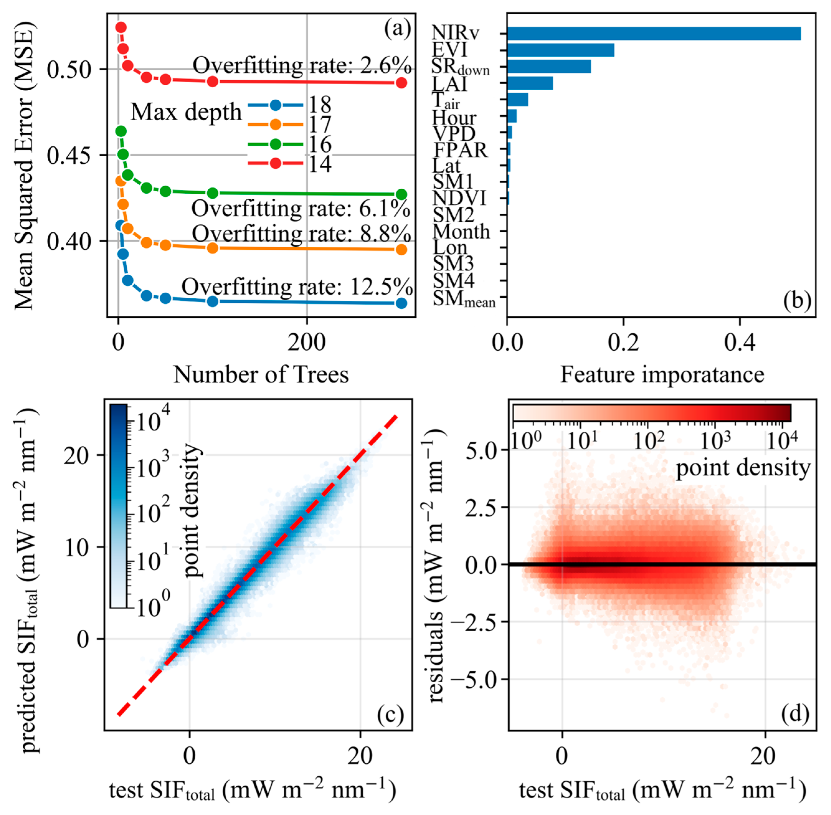
A hyperparameter tuning process was conducted using a grid search with 5-fold cross-validation. The search aimed to balance model complexity with predictive performance. The grid encompassed a wide range of values for each key parameter as follows: Ntree—values of (3, 5, 10, 30, 50, 100, 300) were tested to ensure model stability without excessive computational cost; Depthmax—values of (14, 16, 17, 18) were evaluated to control overfitting by limiting tree growth; and Maximum features—the search included values from 4 up to the total number of features. The optimal combination that yielded the best cross-validation score had 12 as the maximum number of features. The process of hyperparameter tuning (Ntree and Depthmax) and the resulting model performance during this phase are presented in Figure 2 because they are integral to the development of the method.
As Ntree increases, the mean squared error (MSE) of the model decreases exponentially, and when Ntree is greater than or equal to 100, its effect on the MSE becomes minimal (Figure 2a). Thus, Ntree in the final model was set as 100. As Depthmax increases, MSE decreases almost linearly, accompanied by a rapid increase in the rate of overfitting (Figure 2a). To avoid model overfitting, we limited the rate of overfitting to below 10%, and thus set the Depthmax of the final model to 17. The model with fixed hyperparameters showed that the top six predictors (specifically in order: NIRv, EVI, SRdown, LAI, Tair, and Hour) accounted for over 95% of the total importance (Figure 2b). We also compared the model using only the top six predictors with the model using all of the predictors in terms of performance and computational time. In terms of model performance, the former had an RMSE of 0.4951 and an R2 of 0.9822, while the latter had an RMSE of 0.43 and an R2 of 0.9869. In terms of computational time, the latter took 2.5 times longer than the former, though the total time for the latter was only about 10 h. Ultimately, considering that the model with all of the predictors demonstrated better performance and its computational time remained within an acceptable range, we decided to adopt the full-predictor model as the final model. The scatter plot between the test and predicted sets was distributed around the 1:1 line, with a coefficient of determination (R2) of 0.9869 (Figure 2c). The model errors were mainly distributed between −2 and 2 (mW m−2 nm−1; Figure 2d). To provide further evidence of the model’s robustness, a time-based cross-validation procedure was implemented. This involved withholding data from one complete year (2010) as an independent validation set to assess the model’s performance. The validation results for 2010 showed that the RMSE was 0.4491 and the R2 was 0.9847.

2.2.2. Comparison Between SIF Products and EC Flux GPP

Our product SIFtotal_01 and another hourly product, SIFz, were both compared with GPP from EC flux tower sites. We conducted a comparative analysis using linear regression, with the main evaluation metrics including MSE, mean absolute error (MAE), root mean squared error (RMSE), R2, as well as the slope and intercept of the linear model.

2.2.3. Analysis of the Afternoon Depression of Photosynthesis

The afternoon depression of photosynthesis can be reflected either by GPP in the afternoon being lower than in the morning, or by changes in the relationship between GPP and SIF between morning and afternoon [14]. At the site scale, the afternoon depression of photosynthesis for all of the vegetation types and for specific vegetation types was analyzed by comparing the linear slope of GPP-SIFtotal_01 between morning and afternoon. At the global scale, this study examined the afternoon depression of photosynthesis by using the difference in SIF between afternoon and morning, and analyzed its underlying causes by examining the differences in APAR and SIF yield (ΦSIF) between afternoon and morning.

3. Results

3.1. Relationship Between SIF and GPP

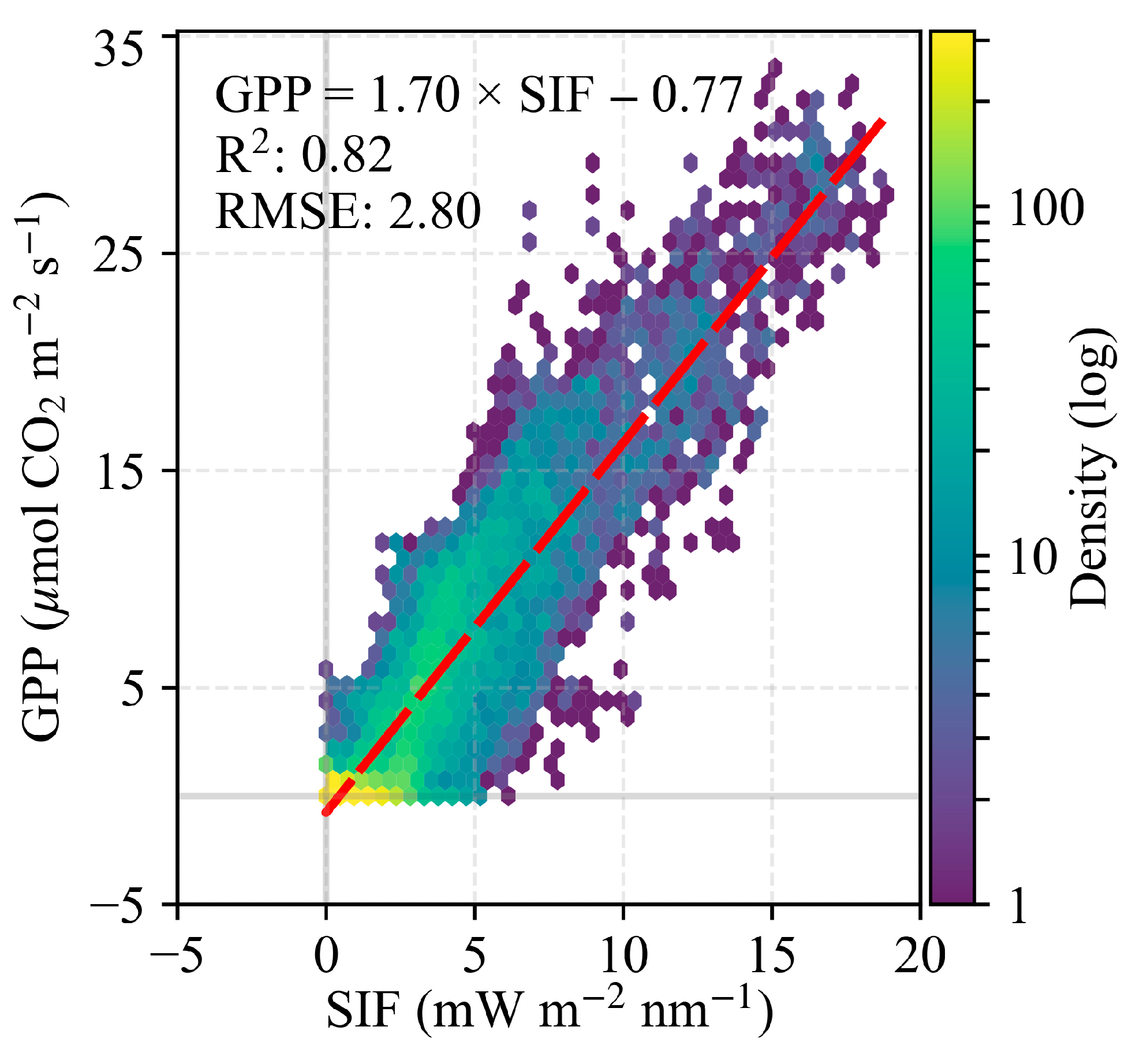
We first examined the relationship between SIFtotal_01 and the GPP in FLUXNET2015 for all 19 of the EC flux sites (Figure 3). In general, a strong linear relationship was observed between SIFtotal_01 and GPP. The regression analysis yielded a slope of 1.70 and an intercept of −0.77, with a R2 of 0.82 and a RMSE of 2.80 mW m−2 nm−1. The hexbin distribution further showed that the majority of data points were concentrated along the regression line, particularly at low-to-moderate values of GPP and SIFtotal_01, suggesting a consistent scaling relationship across different productivity levels. More statistical metrics are presented in Table 1. The MSE and MAE in the SIFtotal_01-GPP relationship were 7.83 and 2.12, respectively.
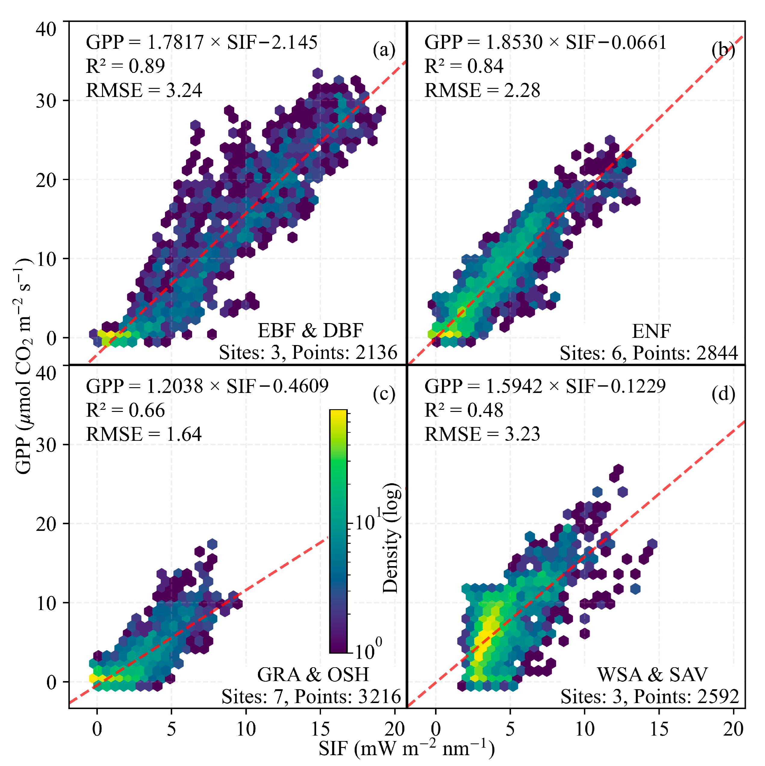
We also analyzed the differences in the relationship between SIFtotal_01 and GPP across different vegetation types (Figure 4). In the EBF and DBF land cover types (Figure 4a), GPP showed a strong positive correlation with SIF (GPP = 1.782 × SIF −2.145, R2 = 0.89, RMSE = 3.24; 3 sites, 2136 points). The ENF land cover type (Figure 4b) exhibited a similarly strong relationship (GPP = 1.853 × SIF −0.066, R2 = 0.84, RMSE = 2.28; six sites, 2844 points). In the GRA and OSH land cover types (Figure 4c), the correlation was moderate (GPP = 1.204 × SIF −0.461, R2 = 0.66, RMSE = 1.64; seven sites, 3216 points), while in the WSA and SAV land cover types (Figure 4d), the correlation was weaker (GPP = 1.594 × SIF −0.123, R2 = 0.48, RMSE = 3.23; three sites, 2592 points).
Compared with the original SIFtotal, our SIFtotal_01 product showed a closer relationship with FLUXNET2015 GPP across all of the land cover types, with the MSE, MAE, and RMSE decreasing by approximately 0.5, 0.13, and 0.1, respectively (Table 1). Further, the regression line of SIFtotal_01 versus GPP is closer to the coordinate origin. When examining specific biome groups, the differences between the two SIF products become more apparent. For the EBF and DBF land cover types, SIFtotal_01 demonstrated superior performance, with lower MSE (3.09 vs. 5.39), MAE (1.43 vs. 1.96), and RMSE (1.76 vs. 2.32), while also achieving a higher R2 (0.89 vs. 0.80). Similarly, for the GRA and OSH land cover types, SIFtotal_01 outperformed SIFtotal, showing lower errors (MSE: 2.7 vs. 3.05; MAE: 1.19 vs. 1.31; RMSE: 1.64 vs. 1.75) and a slightly higher R2 (0.66 vs. 0.64). For the WSA and SAV land cover types, SIFtotal_01 again showed a marginal advantage, with lower error values (MSE: 10.46 vs. 10.84; MAE: 2.58 vs. 2.65; RMSE: 3.23 vs. 3.29) and a slightly higher R2 (0.49 vs. 0.46). However, the intercept for SIFtotal was positive (0.28) when compared with −0.12 for SIFtotal_01. In contrast, for the ENF land cover types, both SIF metrics performed almost equally well, with nearly identical R2 (0.84), RMSE (2.28 vs. 2.24), and MAE (1.76 vs. 1.77). The slope of the regression is also very similar (~1.85), though SIFtotal shows a slightly more favorable intercept closer to zero.
The summer diurnal dynamics of the activity of vegetation in the Haibei-Steppe region were examined using normalized GPP and two SIF products (SIFz and SIFtotal_01, Figure 5). The time series analysis (Figure 5a) revealed that all three indicators exhibited similar diurnal and seasonal patterns, with higher values in July and August and lower values in June, indicating strong temporal synchrony exists between GPP and SIF. The SIFz displayed highly symmetric bell-shaped diurnal variations, whereas the shapes of GPP and SIFtotal_01 were more closely aligned. Scatter plot analyses quantified the relationships between normalized GPP and normalized SIF during morning and afternoon periods (Figure 5b–e). In the morning, GPP was strongly correlated with SIFz (GPP = 0.88 × SIFz + 0.01, R2 = 0.90, RMSE = 0.08; Figure 5b) and slightly less correlated with SIFtotal_01 (GPP = 0.87 × SIFtotal_01 −0.16, R2 = 0.78, RMSE = 0.12; Figure 5c). In the afternoon, the correlation between GPP and SIFz weakened substantially (GPP = 0.77 × SIFz + 0.19, R2 = 0.59, RMSE = 0.15; Figure 5d), whereas GPP-SIFtotal_01 relationships remained strong (GPP = 0.83 × SIFtotal_01 + 0.11, R2 = 0.77, RMSE = 0.11; Figure 5e). These results indicate that SIFtotal_01 provides a more consistent proxy of GPP across diurnal periods, while SIFz is more strongly coupled with morning GPP but less reliable in the afternoon.

3.2. SIF-Indicated Afternoon Depression of Photosynthesis

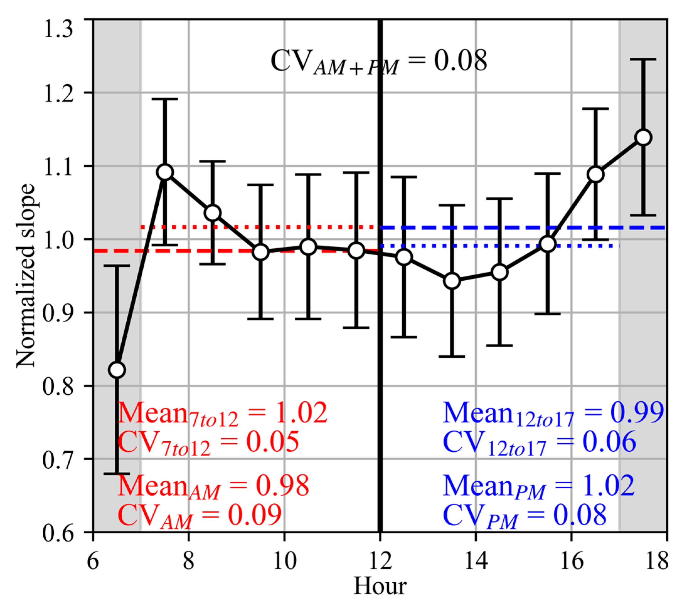
The diurnal variation in the normalized slope for all 19 EC flux sites exhibited clear temporal patterns (Figure 6). The combined AM+PM dataset yielded a coefficient of variation (CV) of 0.08. The values started relatively low at 6:00 (~0.82), increased sharply to a morning peak around 7:00–8:00 (~1.09), and then declined gradually to about 1.0 by midday. A trough was observed between 12:00–14:00 (~0.95), followed by a recovery toward a second peak near 18:00 (~1.13). This double-peak pattern suggests distinct morning and afternoon dynamics are occurring. Statistical metrics revealed distinct morning and afternoon differences. For the entire morning (6:00–12:00), the mean normalized slope was 0.98 with a CV of 0.09, while the afternoon (12:00–18:00) showed a slightly higher mean of 1.02 with a CV of 0.08. However, at the boundaries of daytime, the values were notably lower at 6:00–7:00 and higher again at 17:00–18:00, reflecting transitional conditions. Excluding the transitional periods at the beginning and end of the daytime, a focused comparison between 7:00–12:00 and 12:00–17:00 showed that the morning mean (1.02, CV = 0.05) consistently exceeded the afternoon mean (0.99, CV = 0.06). This asymmetric pattern, where slope values in the afternoon were consistently lower than those at the corresponding hours before noon, indicates the occurrence of an afternoon depression of photosynthesis.
The diurnal dynamics of the normalized slope exhibited distinct differences among land cover groups (Figure 7). All of the groups showed a double-peak pattern, but the relative magnitudes of morning and afternoon values varied. For the EBF and DBF land cover types (three sites, Figure 7a), the overall variability was moderate (CVAM+PM = 0.18). In this group, normalized slope values were consistently higher in the afternoon than in the morning, regardless of whether transitional periods were included. This pattern diverges from the expected afternoon depression of photosynthesis. For the ENF land cover (six sites, Figure 7b), the diurnal variability was lowest of all land cover types (CVAM+PM = 0.06). Here, morning values were consistently higher than afternoon values. The contrast became more pronounced when excluding transitional periods. For the GRA and OSH land cover types (seven sites, Figure 7c), the variability was intermediate (CVAM+PM = 0.13). Mean values for the full morning (6–12 h) and afternoon (12–18 h) were 0.97 and 1.03, respectively. When transitional periods were excluded, the morning mean (1.05) still slightly exceeded the afternoon mean (1.03), indicating a weaker but observable midday asymmetry. For the WSA and SAV land cover types (three sites, Figure 7d), the highest variability was observed among all land cover types (CVAM+PM = 0.25). In this group, normalized slope values were consistently higher in the morning than in the afternoon, regardless of period definition. The contrast was more evident after excluding transitional periods, providing strong evidence of an afternoon depression of photosynthesis.
Figure 8 shows the spatial distribution of SIFtotal_01 at 11:00–12:00 in July 2008, as well as the temporal variations of SIFtotal_01 and GPP at EC flux sites with available observations in 2008. In terms of spatial distribution, SIFtotal_01 was particularly high in low-latitude regions (30°S–30°N), including Central America, the Amazon basin of South America, the southern Sahel and the Congo basin in Africa, and in parts of Southeast Asia, as well as in parts of other mid-latitude regions (30°N–60°N), such as monsoon areas of the Pacific and Atlantic and boreal forests. The SIFtotal_01 exhibited moderate values in low-latitude tropical grasslands, temperate grasslands in the mid-latitudes, and high-latitude regions (>60°N). Meanwhile, SIFtotal_01 was relatively low in arid regions. The afternoon depression of photosynthesis and the seasonal dynamics of photosynthesis can be observed both from the GPP data at the sites shown at the bottom of Figure 8 and from the SIFtotal_01 data displayed at the top of Figure 8.

3.3. Drivers of the Diurnal Dynamics of SIF

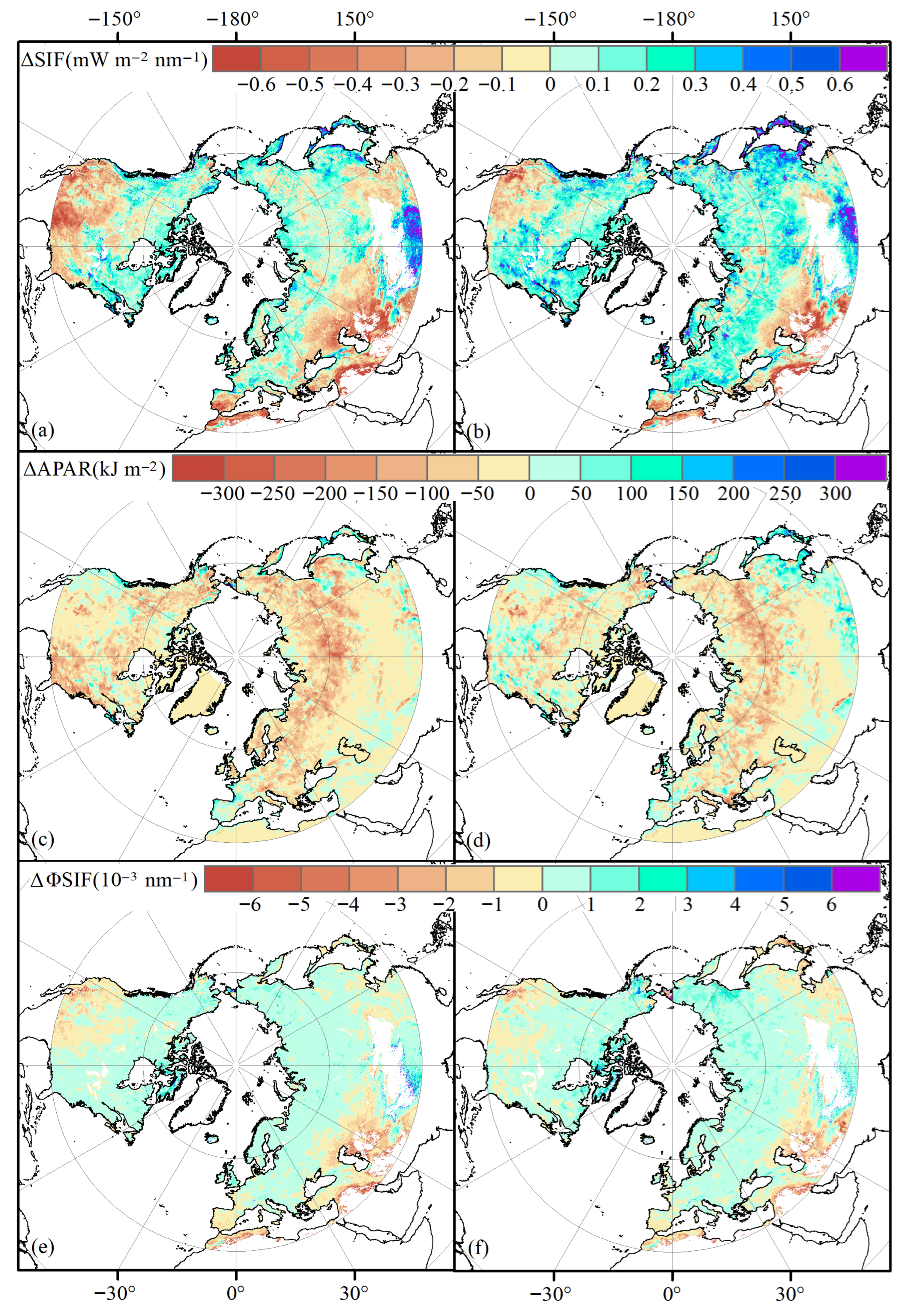
To quantify the influence of soil moisture, we contrasted the diurnal cycles of SIFtotal_01, APAR, and ΦSIF during the wettest and driest years on record for each grid in the mid- to high-latitudes of the Northern Hemisphere (MHNH, Figure 9). For the entire MHNH region, the mean afternoon–morning difference in SIFtotal_01 (ΔSIFtotal_01 = SIFtotal_01PM −SIFtotal_01AM) was about 0.015 (mW m−2 nm−1) in the driest years, whereas it increased to about 0.10 (mW m−2 nm−1) in the wettest years (Figure 9a,b). The ΔSIFtotal_01 exhibited a clear latitudinal pattern in both driest and wettest year; regions north of 50°N were dominated by a positive ΔSIFtotal_01, whereas regions south of 50°N were characterized by a negative ΔSIFtotal_01. In addition, higher values for the afternoon SIFtotal_01 relative to morning values was also observed in Northeast Asia and the Tibetan Plateau. It was also observed that the regions with the smallest ΔSIFtotal_01 (dark brown areas) were mainly located in temperate grasslands and deserts. We also partitioned ΔSIFtotal_01 into ΔAPAR and ΔΦSIF (where ΦSIF = SIFtotal_01/APAR) to highlight their impact on ΔSIFtotal_01. The average ΔAPAR of the entire MHNH region was approximately −323 (kJ m−2) in the driest year, whereas it was around −201 (kJ m−2) in the wettest year (Figure 9c,d). A consistent spatial pattern of ΔAPAR between the driest and wettest years was found; the APAR increased from morning to afternoon in low latitudes but decreased in high latitudes. We further found that the average ΔΦSIF over the entire MHNH region was approximately 0.17 × 10⁻³ nm−1 in the driest year and about 0.36 × 10⁻³ nm−1 in the wettest year (Figure 9e,f). The spatial pattern of ΔΦSIF was consistent with that of ΔSIFtotal_01, being positive mainly in regions north of 50°N, the Tibetan Plateau, and Northeast Asia, and negative primarily in temperate grasslands and desert areas south of 50°N.

4. Discussion

This study successfully downscaled the 0.5° SIFtotal product to a finer resolution of 0.1°, producing the SIFtotal_01 product. It was observed that SIFtotal_01 serves as a more robust indicator of GPP when compared with SIFtotal across various land cover types. Further, the research showed that a biome-dependent depression of photosynthesis exists during the afternoon. The study also demonstrated that factors such as SM, APAR, and ΦSIF collectively influence the diurnal dynamics of SIFtotal_01.

4.1. The Relationship Between GPP and SIFtotal_01, SIFtotal and SIFinstant

The superior performance of SIFtotal_01 when compared with SIFtotal emphasizes the significance of spatial resolution in characterizing the relationship between SIF and GPP. At a coarse resolution of 0.5°, grid cells often span multiple land cover types. This results in heterogeneous canopy structures and mixed signals within a single grid cell, thereby reducing the apparent correlation between SIF and GPP [22,23,24]. By downscaling to 0.1°, SIFtotal_01 better captures the characteristics of the local vegetation community characteristics and aligns more closely with the representative footprint of EC flux sites, thereby reducing scale mismatches and improving data comparability. This is consistent with the viewpoint proposed by previous studies, which suggests that the relationship between SIFtotal and GPP strengthens as the footprint of SIFtotal decreases, and the relationship is best when the footprints of SIFtotal and GPP are aligned [45].
When comparing SIFz with SIFtotal_01, the latter exhibited a more stable and robust relationship with GPP when the two were viewed at the same spatial resolution. This difference can be attributed to the fact that SIFz corresponds to the SIF signal as it is directly observed by the sensor. Sensor-observed SIF is inherently influenced by various factors such as canopy structural heterogeneity, observation geometry, and solar-target-viewing angles [33,46,47]. Thus, the relationship between the sensor-observed SIF and GPP depends on both illumination and observation geometry [48]. In contrast, SIFtotal_01 is derived from SIFtotal representing the total SIF emitted by the canopy. In addition, SIFtotal_01 undergoes corrections for solar viewing geometry and canopy structure effects based on spectral invariance theory [14,49]. Previous research has indicated that normalizing SIF to a standard viewing geometry or differentiating between the contributions of sunlit and shaded leaves enhances the accuracy of GPP estimation [50]. This aligns with our observation that SIFtotal_01 reduces structural and angular biases, yielding a regression line that is more proximate to the coordinate origin and demonstrates increased linearity with GPP. However, Liu et al. [51] considered that even after accounting for solar viewing geometry and canopy structure effects via spectral invariance theory, the relationship between GPP and SIFtotal remains dependent on the sensor’s viewing angle.
In addition, the slope of linear regression between SIFtotal_01 and GPP differed with land cover types, where ecosystems with a higher LAI had a steeper slope in the regression line. This indicated that canopy structure is significantly affected the SIFtotal_01-GPP relationship. Liu et al. [52] and Liu et al. [53] also found the non-linearity between SIFtotal and GPP varied across different biomes. Similarly, Liu et al. [51] further pointed out that canopy heterogeneity influenced the SIFtotal-GPP relationship, which was in line with our results regarding the impacts of LAI. On the contrary, Zhang et al. [54] argued the SIFtotal-GPP relationship converged into two separate models for C3 and C4 photosynthetic pathways, while we observed a continuous gradient dependent on land covers rather than a clear division. This apparent discrepancy may be reconciled by considering that the distribution of C3 and C4 plants, which is inherently tied to land cover type, serves as a fundamental driver of the SIF-GPP relationship. Unlike C3 plants, which often exhibit photosynthetic saturation under high light intensity, C4 plants maintain a strong linear relationship between GPP and SIF across a wide range of light conditions [55]. Furthermore, C4 plants typically demonstrate a higher GPP-SIF ratio than C3 plants. This difference can be attributed less to variations in fluorescence yield and more to the greater dynamic range in light use efficiency (LUE) inherent to the C4 pathway [56]. We therefore believe that the relative abundance of C3 and C4 vegetation within different land cover types creates the underlying biochemical gradient that manifests as the land-cover-dependent pattern in our analysis. Consequently, accurately quantifying global GPP from SIF requires integrating the fraction of C3 and C4 vegetation, because this factor critically influences the magnitude and spatial pattern of estimated carbon fluxes [57].

4.2. Afternoon Depression of Photosynthesis

A clear double-peak pattern was observed in the diurnal dynamics of the slope of SIFtotal_01-GPP, with morning slopes being higher than those in the afternoon. This illustrates that an afternoon depression in photosynthesis occurs across most ecosystems. Numerous site-level and satellite studies have reported this phenomenon, with SIFtotal or reconstructed SIF effectively capturing the afternoon depression in photosynthetic activity [14,31,58]. Some research suggests that this depression is more pronounced at noon when compared with depression of photosynthesis occurring the morning and afternoon [14,32,59,60,61]. Our land-cover-specific analysis revealed the ENF, GRA, OSH, WSA, and SAV land cover types consistently exhibited lower afternoon values when compared with morning ones, supporting the existence of photosynthetic afternoon depression under stress conditions. This agrees with previous observations that dryland and grassland ecosystems often show strong midday or afternoon depression that result from water and heat stress, leading to an underestimation of daily SIF and affecting its relationship with GPP [32,62,63]. In contrast, the EBF and DBF sites displayed higher afternoon slopes, diverging from the expected pattern. However, this finding aligns with the site-scale study by Cheng et al. [64], because the slope of the SIF-GPP relationship is driven by PAR [65].
Environmental stress has played a central role in shaping these diurnal patterns. Our results further emphasize the role of SM; ΔSIFtotal_01 values were larger in wet years than in dry years, and were also larger in wet regions than in dry regions. This aligns with previous studies demonstrating that water stress can decouple SIF and GPP [58,66], and proves that the sensitivity of vegetation to drought was higher in dry regions when compared with humid regions [67]. Moreover, the afternoon depression of SIF has been associated with enhanced non-photochemical quenching (NPQ) as plants dissipate excess energy, suggesting a complementary role between SIF and NPQ as indicators of alternative energy pathways [62]. Mechanistically, decompositing ΔSIF into ΔAPAR and ΔΦSIF revealed that both the absorption of radiation by the canopy and fluorescence yield contributed to ΔSIFtotal_01, with ΔΦSIF exhibiting particularly strong spatial correspondence. This agrees with earlier reports that ΦSIF is more responsive to environmental stress than raw SIF [14,31,32,58,59,60]. Besides this, the SIF-GPP link from morning to afternoon is also influenced by other environmental stresses, including excess light, high VPD, and heat stress [61,68]. For example, in Amazonian rainforests, high atmospheric moisture demand in the morning enhances SIF, but suppresses it in the afternoon [69]. The pronounced sensitivity of SIF to this suite of interacting stresses underscores its significant potential for use in detecting and monitoring the impacts of extreme events at sub-daily scales. Our SIFtotal_01 product offers SIF data with a temporal resolution of each hour within a month. This granularity adequately meets the requirements for monitoring various stressors to a certain extent.

4.3. Implications of Monthly Mean Hourly SIFtotal_01 and Future Prospects

Our SIFtotal_01 product has a monthly average hourly time resolution, which may smooth out the short-term physiological responses of ecosystems to environmental stressors such as rapid stomatal closure under high VPD or brief cloud cover. This kind of time averaging essentially reduces the ability of SIF to capture sub-diurnal extremes and instantaneous plant responses, which are crucial for understanding the rapid adjustment of ecosystems to environmental fluctuations.
However, the primary value of the SIFtotal_01 dataset lies in its ability to characterize recurrent diurnal patterns at a high spatial resolution (0.1°) over a multi-decadal period (2000–2022). By focusing on monthly composites, we mitigated the impacts of day-to-day noise, cloud contamination, and sparse satellite sampling, thereby enhancing the robustness of the inferred diurnal cycles for climatological and biogeochemical modeling. Our results demonstrate that even at this temporally aggregated scale, SIFtotal_01 reliably captures key physiological phenomena such as the afternoon depression of photosynthesis, which exhibits consistent patterns across ecosystems and moisture regimes (Figure 6, Figure 7, Figure 8 and Figure 9). This suggests that the dataset is well-suited for analyzing mean diurnal behavior and its seasonal to interannual variations, particularly in the context of long-term carbon cycle studies, model evaluation, and even ecological restoration evaluation [70]. Further, many critical types of environmental stress, such as drought, develop and persist over timescales of weeks to months [30]. The monthly mean hourly data are therefore particularly adept at capturing the sustained impact of such stresses on vegetation activity, because they effectively integrate the diurnal response patterns of ecosystems over the duration of the stress event, providing a more stable and representative signal than daily snapshots which can be highly variable.
Looking forward, the increasing availability of high-frequency SIF observations from OCO-3 and geostationary satellites (e.g., Geo Kompsat-2A, Geostationary Operational Environmental Satellite-R, Fengyun-4) opens promising avenues for downscaling to daily or even sub-daily resolutions [9,10,11,12]. Such an effort would require integrating SIF retrievals with concurrent meteorological drivers (e.g., from ERA5-Land), land surface properties, and deep learning techniques capable of resolving non-linear diurnal interactions [32]. For instance, a hybrid approach combining the multi-angle sampling of OCO-3 with the high temporal cadence of geostationary data could help reconstruct half-hourly SIF fields [31]. However, challenges remain, including the need for rigorous angular normalization, gap-filling under cloudy conditions, and reconciling spatial and spectral differences among sensors.

4.4. Limitations and Applications

Several limitations of this study should be acknowledged. First, despite the improvement in spatial resolution from 0.5° to 0.1°, the downscaled SIF product (SIFtotal_01) still does not perfectly match the footprint of eddy covariance flux towers, which may introduce uncertainties when validating site-level processes. Second, although we carefully filtered the FLUXNET2015 dataset, the selected flux sites do not represent all of the land-cover types, limiting the generalizability of the SIF–GPP relationship across ecosystems. Third, the mechanisms underlying the afternoon depression of photosynthesis remain incompletely understood, particularly regarding its interactions with multiple environmental stresses beyond water availability. Fourth, the limited availability of eddy covariance flux towers within C4-dominated ecosystems posed a significant challenge, preventing a robust explanation of how C4 photosynthesis modulates the SIF-GPP relationship. Finally, the current product has not explicitly accounted for the impact of clouds, which is a notable limitation. Cloud contamination can distort the diurnal SIF signal by attenuating the incoming solar radiation and consequently suppressing the observed magnitude of SIF. This effect is particularly pronounced in humid regions characterized by frequent and persistent cloud cover, potentially leading to an underestimation of daily photosynthetic activity and obscuring the true diurnal cycle. Future versions of the product could benefit significantly from incorporating a cloud-adjusted SIF retrieval, for instance, by leveraging concurrent meteorological data or radiative transfer models to correct for the radiative transfer effects under cloudy conditions.
Despite these limitations, the SIFtotal_01 dataset developed here provides several important applications. Its global coverage and long temporal span (2000–2022) make it a valuable resource for monitoring spatiotemporal variations in terrestrial photosynthesis and carbon fluxes. The dataset can support investigations of ecosystem productivity at regional to global scales, complementing flux tower observations and bridging the gap between site-level measurements and satellite-based assessments. Further, SIFtotal_01 can serve as a benchmark for evaluating dynamic global vegetation models and earth system models by providing observational constraints on photosynthetic efficiency and diurnal dynamics. The ability to analyze diurnal variations in photosynthesis, such as the afternoon depression of photosynthesis, also highlights its potential for improving our understanding of plant stress responses under changing climatic conditions. In addition, the dataset could inform applied domains, such as agricultural monitoring, drought early warning, and climate–carbon feedback assessments, offering insights into both short-term anomalies and long-term ecosystem trajectories.

5. Conclusions

In this study, we developed a random forest-based downscaling framework to generate a global 0.1° SIF dataset (SIFtotal_01) from the coarse-resolution (0.5°) SIFtotal product for the period 2000–2022. The SIFtotal_01 dataset was evaluated against eddy covariance GPP observations and demonstrated improved performance in representing site-level variations compared with existing satellite-based datasets. By analyzing the SIF-GPP relationships across different land-cover types, we showed that SIFtotal_01 captured a distinct double-peak pattern in the diurnal dynamics of the SIFtotal_01–GPP slope, with consistently higher slopes in the morning than in the afternoon, reflecting an afternoon depression of photosynthesis across most ecosystems. The SM was found to modulate the afternoon depression, and ΦSIF exhibited a stronger sensitivity than APAR, emphasizing its potential as a diagnostic indicator of water-stress-induced afternoon photosynthetic depression. While limitations remain regarding spatial resolution, flux tower representativeness, and the treatment of cloud contamination, SIFtotal_01 provides a long-term (2000–2022), global, monthly mean hourly SIF dataset at a 0.1° resolution. With its ability to capture both ecosystem-level photosynthetic processes and diurnal physiological dynamics, SIFtotal_01 offers new opportunities for evaluating earth system models, improving the large-scale assessments of vegetation stress responses, and supporting applications in agriculture, drought monitoring, and climate–carbon feedback research.

Author Contributions

Conceptualization, Y.L. and Z.Z.; methodology, Y.L.; software, Y.L.; validation, D.Z. and Y.Z.; formal analysis, Y.L.; investigation, D.Z.; resources, Y.Z.; data curation, Y.L.; writing—original draft preparation, Y.L.; writing—review and editing, Z.Z.; visualization, Y.L.; supervision, Z.Z.; project administration, Y.L.; funding acquisition, Y.L. All authors have read and agreed to the published version of the manuscript.

Funding

This research was funded by National Natural Science Foundation of China under Grants 42201398, the Startup Foundation for Introducing Talent of NUIST under Grant 2023r010. Natural Science Foundation of Jiangsu Province (BK20240068), and Scientific and Technological Innovation Foundation of Inner Mongolia Meteorological Bureau (nmqxkjcx202528).

Data Availability Statement

The Global 0.1-degree monthly mean hourly total canopy solar-induced chlorophyll fluorescence dataset (SIFtotal_01) generated in this study will be made publicly available upon publication through the [National Ecosystem Research Network of China] repository. The DOI link will be provided here once it is assigned. The website of our team on the National Ecosystem Research Network of China is https://www.nesdc.org.cn/otherProject/index?menuId=team&projectId=1328.

Acknowledgments

All authors approval this paper submission to Remote Sensing and declare no conflict of interest. This research is financially supported by the National Natural Science Foundation of China under Grant 42201398. The eddy covariance data used in this study was acquired and shared by the FLUXNET community, including the following networks: AmeriFlux, AfriFlux, AsiaFlux, CarboAfrica, CarboEuropeIP, CarboItaly, CarboMont, ChinaFlux, Fluxnet-Canada, GreenGrass, ICOS, KoFlux, LBA, NECC, OzFlux-TERN, TCOS-Siberia, and USCCC. The authors acknowledge all data producers. We would also like to thank Tommy Taylor, Nick Parazoo, and Abishek Chatterjee for making OCO-3 SIF data publicly available. We greatly appreciate the anonymous reviewers for their insightful and constructive comments that helped us to improve our manuscript. We thank LetPub (www.letpub.com.cn) for its linguistic assistance during the preparation of this manuscript.

Conflicts of Interest

The authors declare no conflicts of interest.

Abbreviations

The following abbreviations are used in this manuscript:
APARAbsorbed photosynthetic active radiation
CO2Carbon dioxide
CVCoefficient of variation
DBFDeciduous broadleaved forests
DepthmaxMax depth of a tree
EBFEvergreen broadleaved forests
ECEddy covariance
ENFEvergreen Needleleaf forests
ERA5The fifth generation of European reanalysis
EVIEnhanced vegetation index
FPARFraction of absorbed photosynthetic active radiation
GPPGross primary productivity
GRAGrasslands
LAILeaf area index
MAEMean absolute error
MHNHMid- to high-latitudes of the Northern Hemisphere
MODISModerate-resolution imaging spectroradiometer
MSEMean squared error
NDVINormalized difference vegetation index
NIRvNear-infrared reflectance of vegetation
NtreeNumber of trees
OCOOrbiting the Carbon Observatory
OSHOpen shrublands
PARPhotosynthetic active radiation
R2Goodness of fit
RFRandom forest
RMSERoot mean square error
RSRemote sensing
SAVSavannas
SDStandard deviation
SIFSolar-induced chlorophyll fluorescence
SIFinstantInstantaneous SIF
SIFnadirNadir-viewing SIF
SIFtotal_01Downscaled monthly mean diurnal SIFtotal product at 0.1° resolution produced in this study
SIFtotalTotal canopy SIF emission (dataset)
SIFzSIFinstant dataset produced by Dayang Zhao
SMSoil moisture
SMmeanThe mean values of the four-layer SM
SMnThe SM in the n layer (n = 1, 2, 3, 4)
SRdownSurface solar radiation downward
TairAir temperature
TdewDew point temperature
VPDVapor pressure deficit
WSAWoody Savannas
ΔAPARThe afternoon–morning APAR difference
ΔSIFtotal_01The afternoon–morning SIFtotal_01 difference
ΔΦSIFThe afternoon–morning ΦSIF difference
ΦSIFSIF yield

Appendix A

Appendix A.1

Table A1. List of the data used in this study.
Data NameDescriptionTemporal ResolutionSpatial ResolutionSourcePurpose in This Study
SIFtotalTotal canopy SIF emission retrieval from [14]Monthly mean hourly, 2000~20220.5 degreehttps://doi.org/10.12199/nesdc.ecodb.rs.2024.029 (accessed on 18 July 2025)Raw data used for downscaling
SIFzDiurnal SIF dataset produced by [32]Hourly, only in June–August of 2019~20220.05 degreeObtain from co-authorsCompare with our downscaled dataset SIFtotal_01
GPP from FLUXNET2015Reference GPP extracted from the half-hourly data of FLUXNET2015Half hourlySite scalehttps://fluxnet.org/ (accessed on 31 July 2025)Compare with our downscaled dataset SIFtotal_01
GPP from Haibei steppe EC flux stationReference GPP extracted from the half-hourly data of Haibei steppe EC flux station in ChinaFLUXHalf hourly, only in 2019–2020Site scalehttps://nesdc.org.cn/sdo/detail?id=64e6cd5e7e2817429fbc7afd (accessed on 31 July 2025)Compare with our downscaled dataset SIFtotal_01
ERA5-LandThe fifth generation of European reanalysis datasetHourly0.1 degreehttps://doi.org/10.24381/cds.e2161bac (accessed on 27 August 2025)Used for RF modeling, wet or dry year determine, and calculating ΦSIF
MODIS MOD13A3MODIS vegetation index dataset16 day1 kmhttps://doi.org/10.5067/MODIS/MOD13A3.061 (accessed on 18 July 2025)Used for RF modeling and Site data filter
MODIS MCD15A3HMODIS LAI and FPAR dataset4 day500 mhttps://doi.org/10.5067/MODIS/MCD15A3H.061 (accessed on 18 July 2025)Used for RF modeling
MODIS MCD12Q1MODIS land cover datasetyearly500 mhttps://doi.org/10.5067/MODIS/MCD12Q1.061 (accessed on 18 July 2025)Used for land cover classification and site filter

Appendix A.2

The overall workflow of this study, encompassing data processing, model development, and analysis, is summarized here.
Figure A1. Flowchart of this study.
Remotesensing 17 03429 g0a1

Appendix A.3

The collinearity of different predictors was obtained here through the correlation coefficients between them.
Figure A2. Correlation matrix heatmap of different predictors.
Remotesensing 17 03429 g0a2

References

  1. Fu, Z.; Stoy, P.; Poulter, B.; Gerken, T.; Zhang, Z.; Wakbulcho, G.; Niu, S. Maximum carbon uptake rate dominates the interannual variability of global net ecosystem exchange. Glob. Change Biol. 2019, 25, 3381–3394. [Google Scholar] [CrossRef]
  2. Sitch, S.; Friedlingstein, P.; Gruber, N.; Jones, S.; Murray-Tortarolo, G.; Ahlström, A.; Doney, S.; Graven, H.; Heinze, C.; Huntingford, C.; et al. Recent trends and drivers of regional sources and sinks of carbon dioxide. Biogeosciences 2015, 12, 653–679. [Google Scholar] [CrossRef]
  3. Lin, C.; Gentine, P.; Frankenberg, C.; Zhou, S.; Kennedy, D.; Li, X. Evaluation and mechanism exploration of the diurnal hysteresis of ecosystem fluxes. Agric. For. Meteorol. 2019, 278, 107642. [Google Scholar] [CrossRef]
  4. Xiao, J.; Fisher, J.; Hashimoto, H.; Ichii, K.; Parazoo, N. Emerging satellite observations for diurnal cycling of ecosystem processes. Nat. Plants 2021, 7, 877–887. [Google Scholar] [CrossRef]
  5. Lasslop, G.; Reichstein, M.; Papale, D.; Richardson, A.; Arneth, A.; Barr, A.; Stoy, P.; Wohlfahrt, G. Separation of net ecosystem exchange into assimilation and respiration using a light response curve approach: Critical issues and global evaluation. Glob. Change Biol. 2010, 16, 187–208. [Google Scholar] [CrossRef]
  6. Schimel, D.; Schneider, F.; Bloom, A.; Bowman, K.; Cawse-Nicholson, K.; Elder, C.; Ferraz, A.; Fisher, J.; Hulley, G.; Liu, J.; et al. Flux towers in the sky: Global ecology from space. New Phytol. 2019, 224, 570–584. [Google Scholar] [CrossRef]
  7. Bodesheim, P.; Jung, M.; Gans, F.; Mahecha, M.; Reichstein, M. Upscaled diurnal cycles of land-atmosphere fluxes: A new global half-hourly data product. Earth Syst. Sci. Data 2018, 10, 1327–1365. [Google Scholar] [CrossRef]
  8. Nelson, J.; Walther, S.; Gans, F.; Kraft, B.; Weber, U.; Novick, K.; Buchmann, N.; Migliavacca, M.; Wohlfahrt, G.; Sigut, L.; et al. X-BASE: The first terrestrial carbon and water flux products from an extended data-driven scaling framework, FLUXCOM-X. Biogeosciences 2024, 21, 5079–5115. [Google Scholar] [CrossRef]
  9. Jeong, S.; Ryu, Y.; Dechant, B.; Li, X.; Kong, J.; Choi, W.; Kang, M.; Yeom, J.; Lim, J.; Jang, K.; et al. Tracking diurnal to seasonal variations of gross primary productivity using a geostationary satellite, GK-2A advanced meteorological imager. Remote Sens. Environ. 2023, 284, 113365. [Google Scholar] [CrossRef]
  10. Khan, A.; Stoy, P.; Joiner, J.; Baldocchi, D.; Verfaillie, J.; Chen, M.; Otkin, J. The Diurnal Dynamics of Gross Primary Productivity Using Observations From the Advanced Baseline Imager on the Geostationary Operational Environmental Satellite-R Series at an Oak Savanna Ecosystem. J. Geophys. Res. Biogeosci. 2022, 127, e2021JG006701. [Google Scholar] [CrossRef]
  11. Li, X.; Ryu, Y.; Xiao, J.; Dechant, B.; Liu, J.; Li, B.; Jeong, S.; Gentine, P. New-generation geostationary satellite reveals widespread midday depression in dryland photosynthesis during 2020 western US heatwave. Sci. Adv. 2023, 9, eadi0775. [Google Scholar] [CrossRef] [PubMed]
  12. Yamamoto, Y.; Ichii, K.; Yang, W.; Shikakura, Y.; Ryu, Y.; Kang, M.; Murayama, S.; Kim, S.; Takao, Y.; Ueyama, M.; et al. Modeling diurnal gross primary production in East Asia using Himawari-8/9 geostationary satellite data. Remote Sens. Environ. 2025, 328, 114866. [Google Scholar] [CrossRef]
  13. Schmit, T.; Griffith, P.; Gunshor, M.; Daniels, J.; Goodman, S.; Lebair, W. A Closer Look at the ABI on the GOES-R Series. Bull. Am. Meteorol. Soc. 2017, 98, 681–698. [Google Scholar] [CrossRef]
  14. Zhang, Z.; Guanter, L.; Porcar-Castell, A.; Rossini, M.; Labrador, J.; Zhang, Y. Global modeling diurnal gross primary production from OCO-3 solar-induced chlorophyll fluorescence. Remote Sens. Environ. 2023, 285, 113383. [Google Scholar] [CrossRef]
  15. Guanter, L.; Zhang, Y.; Jung, M.; Joiner, J.; Voigt, M.; Berry, J.; Frankenberg, C.; Huete, A.; Zarco-Tejada, P.; Lee, J.; et al. Global and time-resolved monitoring of crop photosynthesis with chlorophyll fluorescence. Proc. Natl. Acad. Sci. USA 2014, 111, E1327–E1333. [Google Scholar] [CrossRef]
  16. Porcar-Castell, A.; Malenovsky, Z.; Magney, T.; Van Wittenberghe, S.; Fernández-Marín, B.; Maignan, F.; Zhang, Y.; Maseyk, K.; Atherton, J.; Albert, L.; et al. Chlorophyll a fluorescence illuminates a path connecting plant molecular biology to Earth-system science. Nat. Plants 2021, 7, 998–1009. [Google Scholar] [CrossRef]
  17. Porcar-Castell, A.; Tyystjärvi, E.; Atherton, J.; van der Tol, C.; Flexas, J.; Pfündel, E.; Moreno, J.; Frankenberg, C.; Berry, J. Linking chlorophyll a fluorescence to photosynthesis for remote sensing applications: Mechanisms and challenges. J. Exp. Bot. 2014, 65, 4065–4095. [Google Scholar] [CrossRef]
  18. van der Tol, C.; Berry, J.; Campbell, P.; Rascher, U. Models of fluorescence and photosynthesis for interpreting measurements of solar-induced chlorophyll fluorescence. J. Geophys. Res. Biogeosci. 2014, 119, 2312–2327. [Google Scholar] [CrossRef]
  19. Duveiller, G.; Cescatti, A. Spatially downscaling sun-induced chlorophyll fluorescence leads to an improved temporal correlation with gross primary productivity. Remote Sens. Environ. 2016, 182, 72–89. [Google Scholar] [CrossRef]
  20. Gentine, P.; Alemohammad, S. Reconstructed Solar-Induced Fluorescence: A Machine Learning Vegetation Product Based on MODIS Surface Reflectance to Reproduce GOME-2 Solar-Induced Fluorescence. Geophys. Res. Lett. 2018, 45, 3136–3146. [Google Scholar] [CrossRef]
  21. Zhang, Y.; Joiner, J.; Alemohammad, S.; Zhou, S.; Gentine, P. A global spatially contiguous solar-induced fluorescence (CSIF) dataset using neural networks. Biogeosciences 2018, 15, 5779–5800. [Google Scholar] [CrossRef]
  22. Li, X.; Xiao, J. A Global, 0.05-Degree Product of Solar-Induced Chlorophyll Fluorescence Derived from OCO-2, MODIS, and Reanalysis Data. Remote Sens. 2019, 11, 517. [Google Scholar] [CrossRef]
  23. Yu, L.; Wen, J.; Chang, C.; Frankenberg, C.; Sun, Y. High-Resolution Global Contiguous SIF of OCO-2. Geophys. Res. Lett. 2019, 46, 1449–1458. [Google Scholar] [CrossRef]
  24. Wen, J.; Köhler, P.; Duveiller, G.; Parazoo, N.; Magney, T.; Hooker, G.; Yu, L.; Chang, C.; Sun, Y. A framework for harmonizing multiple satellite instruments to generate a long-term global high spatial-resolution solar-induced chlorophyll fluorescence (SIF). Remote Sens. Environ. 2020, 239, 111644. [Google Scholar] [CrossRef]
  25. Doughty, R.; Köhler, P.; Frankenberg, C.; Magney, T.; Xiao, X.; Qin, Y.; Wu, X.; Moore, B. TROPOMI reveals dry-season increase of solar-induced chlorophyll fluorescence in the Amazon forest. Proc. Natl. Acad. Sci. USA 2019, 116, 22393–22398. [Google Scholar] [CrossRef]
  26. Sun, Y.; Frankenberg, C.; Wood, J.; Schimel, D.; Jung, M.; Guanter, L.; Drewry, D.; Verma, M.; Porcar-Castell, A.; Griffis, T.; et al. OCO-2 advances photosynthesis observation from space via solar-induced chlorophyll fluorescence. Science 2017, 358, eaam5747. [Google Scholar] [CrossRef]
  27. Zhang, Y.; Xiao, X.; Zhang, Y.; Wolf, S.; Zhou, S.; Joiner, J.; Guanter, L.; Verma, M.; Sun, Y.; Yang, X.; et al. On the relationship between sub-daily instantaneous and daily total gross primary production: Implications for interpreting satellite-based SIF retrievals. Remote Sens. Environ. 2018, 205, 276–289. [Google Scholar] [CrossRef]
  28. Doughty, R.; Kurosu, T.; Parazoo, N.; Köhler, P.; Wang, Y.; Sun, Y.; Frankenberg, C. Global GOSAT, OCO-2, and OCO-3 solar-induced chlorophyll fluorescence datasets. Earth Syst. Sci. Data 2022, 14, 1513–1529. [Google Scholar] [CrossRef]
  29. Stavros, E.; Schimel, D.; Pavlick, R.; Serbin, S.; Swann, A.; Duncanson, L.; Fisher, J.; Fassnacht, F.; Ustin, S.; Dubayah, R.; et al. ISS observations offer insights into plant function. Nat. Ecol. Evol. 2017, 1, 0194. [Google Scholar] [CrossRef]
  30. Zhang, Y.; Fang, J.; Smith, W.; Wang, X.; Gentine, P.; Scott, R.; Migliavacca, M.; Jeong, S.; Litvak, M.; Zhou, S. Satellite solar-induced chlorophyll fluorescence tracks physiological drought stress development during 2020 southwest US drought. Glob. Change Biol. 2023, 29, 3395–3408. [Google Scholar] [CrossRef]
  31. Jeong, S.; Ryu, Y.; Li, X.; Dechant, B.; Liu, J.; Kong, J.; Choi, W.; Fang, J.; Lian, X.; Gentine, P. GEOSIF: A continental-scale sub-daily reconstructed solar-induced fluorescence derived from OCO-3 and GK-2A over Eastern Asia and Oceania. Remote Sens. Environ. 2024, 311, 114284. [Google Scholar] [CrossRef]
  32. Zhao, D.; Zhang, Z.; Zhang, Y. Large-scale diurnal responses of solar-induced chlorophyll fluorescence (SIF) to varying heat and water stresses: Implications for monitoring SIF variations from satellite observations. Remote Sens. Environ. 2025, 324, 114748. [Google Scholar] [CrossRef]
  33. Zhang, Z.; Zhang, Y. Solar angle matters: Diurnal pattern of solar-induced chlorophyll fluorescence from OCO-3 and TROPOMI. Remote Sens. Environ. 2023, 285, 113380. [Google Scholar] [CrossRef]
  34. Yang, P.; van der Tol, C. Linking canopy scattering of far-red sun-induced chlorophyll fluorescence with reflectance. Remote Sens. Environ. 2018, 209, 456–467. [Google Scholar] [CrossRef]
  35. Zeng, Y.; Badgley, G.; Dechant, B.; Ryu, Y.; Chen, M.; Berry, J. A practical approach for estimating the escape ratio of near-infrared solar-induced chlorophyll fluorescence. Remote Sens. Environ. 2019, 232, 111209. [Google Scholar] [CrossRef]
  36. Pastorello, G.; Trotta, C.; Canfora, E.; Chu, H.; Christianson, D.; Cheah, Y.; Poindexter, C.; Chen, J.; Elbashandy, A.; Humphrey, M.; et al. The FLUXNET2015 dataset and the ONEFlux processing pipeline for eddy covariance data. Sci. Data 2020, 7, 225. [Google Scholar] [CrossRef]
  37. Chu, H.; Luo, X.; Ouyang, Z.; Chan, W.; Dengel, S.; Biraud, S.; Torn, M.; Metzger, S.; Kumar, J.; Arain, M.; et al. Representativeness of Eddy-Covariance flux footprints for areas surrounding AmeriFlux sites. Agric. For. Meteorol. 2021, 301, 108350. [Google Scholar] [CrossRef]
  38. Muñoz-Sabater, J.; Dutra, E.; Agustí-Panareda, A.; Albergel, C.; Arduini, G.; Balsamo, G.; Boussetta, S.; Choulga, M.; Harrigan, S.; Hersbach, H.; et al. ERA5-Land: A state-of-the-art global reanalysis dataset for land applications. Earth Syst. Sci. Data 2021, 13, 4349–4383. [Google Scholar] [CrossRef]
  39. Alduchov, O.A.; Eskridge, R.E. Improved Magnus form approximation of saturation vapor pressure. J. Appl. Meteorol. (1988–2005) 1996, 35, 601–609. [Google Scholar] [CrossRef]
  40. Didan, K. MODIS/Terra Vegetation Indices Monthly L3 Global 1 km SIN Grid V061 [Data set]; NASA Land Processes Distributed Active Archive Center: Sioux Falls, SD, USA, 2021. [Google Scholar] [CrossRef]
  41. Badgley, G.; Field, C.; Berry, J. Canopy near-infrared reflectance and terrestrial photosynthesis. Sci. Adv. 2017, 3, e1602244. [Google Scholar] [CrossRef] [PubMed]
  42. Myneni, R.; Knyazikhin, Y.; Park, T. MODIS/Terra+Aqua Leaf Area Index/FPAR 4-Day L4 Global 500 m SIN Grid V061 [Data set]; NASA Land Processes Distributed Active Archive Center: Sioux Falls, SD, USA, 2021. [Google Scholar] [CrossRef]
  43. Friedl, M.; Sulla-Menashe, D. MODIS/Terra+Aqua Land Cover Type Yearly L3 Global 500 m SIN Grid V061 [Data set]; NASA Land Processes Distributed Active Archive Center: Sioux Falls, SD, USA, 2022. [Google Scholar] [CrossRef]
  44. Breiman, L. Random Forests. In Machine Learning; Elsevier: Amsterdam, The Netherlands, 2001; Volume 45, pp. 5–32. [Google Scholar]
  45. Zhang, Z.; Zhang, Y.; Zhang, Y. Generating high-resolution total canopy SIF emission from TROPOMI data: Algorithm and application. Remote Sens. Environ. 2023, 295, 113699. [Google Scholar] [CrossRef]
  46. Morozumi, T.; Kato, T.; Kobayashi, H.; Sakai, Y.; Nakashima, N.; Buareal, K.; Nasahara, K.; Akitsu, T.; Murayama, S.; Noda, H.; et al. Contributions of the understory and midstory to total canopy solar-induced chlorophyll fluorescence in a ground-based study in conjunction with seasonal gross primary productivity in a cool-temperate deciduous broadleaf forest. Remote Sens. Environ. 2023, 284, 113340. [Google Scholar] [CrossRef]
  47. Zhang, Z.; Chen, J.; Guanter, L.; He, L.; Zhang, Y. From Canopy-Leaving to Total Canopy Far-Red Fluorescence Emission for Remote Sensing of Photosynthesis: First Results From TROPOMI. Geophys. Res. Lett. 2019, 46, 12030–12040. [Google Scholar] [CrossRef]
  48. Zhang, Z.; Zhang, Y.; Zhang, Q.; Chen, J.; Porcar-Castell, A.; Guanter, L.; Wu, Y.; Zhang, X.; Wang, H.; Ding, D.; et al. Assessing bi-directional effects on the diurnal cycle of measured solar-induced chlorophyll fluorescence in crop canopies. Agric. For. Meteorol. 2020, 295, 108147. [Google Scholar] [CrossRef]
  49. Liu, W.; Luo, S.; Lu, X.; Atherton, J.; Gastellu-Etchegorry, J. Simulation-Based Evaluation of the Estimation Methods of Far-Red Solar-Induced Chlorophyll Fluorescence Escape Probability in Discontinuous Forest Canopies. Remote Sens. 2020, 12, 3962. [Google Scholar] [CrossRef]
  50. Zhang, Z.; Chen, J.; Zhang, Y.; Li, M. Improving the ability of solar-induced chlorophyll fluorescence to track gross primary production through differentiating sunlit and shaded leaves. Agric. For. Meteorol. 2023, 341, 109658. [Google Scholar] [CrossRef]
  51. Liu, W.; Atherton, J.; Mottus, M.; Malenovsky, Z.; Luo, S.; Zhang, Y.; Gastellu-Etchegorry, J. Analysing far-red SIF directional anisotropy of three structurally contrasting forest canopies towards improved GPP estimation. Agric. For. Meteorol. 2023, 338, 109531. [Google Scholar] [CrossRef]
  52. Liu, Y.; Chen, J.; He, L.; Zhang, Z.; Wang, R.; Rogers, C.; Fan, W.; de Oliveira, G.; Xie, X. Non-linearity between gross primary productivity and far-red solar-induced chlorophyll fluorescence emitted from canopies of major biomes. Remote Sens. Environ. 2022, 271, 112896. [Google Scholar] [CrossRef]
  53. Liu, L.; Zhao, W.; Shen, Q.; Wu, J.; Teng, Y.; Yang, J.; Han, X.; Tian, F. Nonlinear Relationship Between the Yield of Solar-Induced Chlorophyll Fluorescence and Photosynthetic Efficiency in Senescent Crops. Remote Sens. 2020, 12, 1518. [Google Scholar] [CrossRef]
  54. Zhang, Z.; Zhang, Y.; Porcar-Castell, A.; Joiner, J.; Guanter, L.; Yang, X.; Migliavacca, M.; Ju, W.; Sun, Z.; Chen, S.; et al. Reduction of structural impacts and distinction of photosynthetic pathways in a global estimation of GPP from space-borne solar-induced chlorophyll fluorescence. Remote Sens. Environ. 2020, 240, 111722. [Google Scholar] [CrossRef]
  55. He, L.; Magney, T.; Dutta, D.; Yin, Y.; Köhler, P.; Grossmann, K.; Stutz, J.; Dold, C.; Hatfield, J.; Guan, K.; et al. From the Ground to Space: Using Solar-Induced Chlorophyll Fluorescence to Estimate Crop Productivity. Geophys. Res. Lett. 2020, 47, e2020GL087474. [Google Scholar] [CrossRef]
  56. Liu, L.; Guan, L.; Liu, X. Directly estimating diurnal changes in GPP for C3 and C4 crops using far-red sun-induced chlorophyll fluorescence. Agric. For. Meteorol. 2017, 232, 1–9. [Google Scholar] [CrossRef]
  57. MacBean, N.; Maignan, F.; Bacour, C.; Lewis, P.; Peylin, P.; Guanter, L.; Köhler, P.; Gómez-Dans, J.; Disney, M. Strong constraint on modelled global carbon uptake using solar-induced chlorophyll fluorescence data. Sci. Rep. 2018, 8, 1973. [Google Scholar] [CrossRef] [PubMed]
  58. Pan, Q.; Cheng, X.; Hu, M.; Liu, L.; Wang, X.; Zhang, J.; Li, Z.; Yuan, W.; Gao, X. The Afternoon/Morning Ratio of Tower-Based Solar-Induced Chlorophyll Fluorescence Can Be Used to Monitor Drought in a Chinese Cork Oak Plantation. Remote Sens. 2024, 16, 1897. [Google Scholar] [CrossRef]
  59. Lin, J.; Zhou, L.; Wu, J.; Han, X.; Zhao, B.; Chen, M.; Liu, L. Water stress significantly affects the diurnal variation of solar-induced chlorophyll fluorescence (SIF): A case study for winter wheat. Sci. Total Environ. 2024, 908, 168256. [Google Scholar] [CrossRef] [PubMed]
  60. Liu, Z.; He, X.; Yang, P.; Jiang, H.; Xu, S.; Zhao, H.; Ren, S.; Chen, M. Diurnal Pattern of Sun-Induced Chlorophyll Fluorescence as Reliable Indicators of Crop Water Stress. IEEE Geosci. Remote Sens. Lett. 2023, 20, 1–5. [Google Scholar] [CrossRef]
  61. Zhu, X.; Hou, Y.; Zhang, Y.; Lu, X.; Liu, Z.; Weng, Q. Potential of Sun-Induced Chlorophyll Fluorescence for Indicating Mangrove Canopy Photosynthesis. J. Geophys. Res. Biogeosci. 2021, 126, e2020JG006159. [Google Scholar] [CrossRef]
  62. Paul-Limoges, E.; Damm, A.; Hueni, A.; Liebisch, F.; Eugster, W.; Schaepman, M.; Buchmann, N. Effect of environmental conditions on sun-induced fluorescence in a mixed forest and a cropland. Remote Sens. Environ. 2018, 219, 310–323. [Google Scholar] [CrossRef]
  63. Qiu, R.; Han, G.; Li, X.; Xiao, J.; Liu, J.; Wang, S.; Li, S.; Gong, W. Contrasting responses of relationship between solar-induced fluorescence and gross primary production to drought across aridity gradients. Remote Sens. Environ. 2024, 302, 113984. [Google Scholar] [CrossRef]
  64. Cheng, X.; Hu, M.; Zhou, Y.; Wang, F.; Liu, L.; Wang, Y.; Huang, H.; Zhang, J. The divergence of micrometeorology sensitivity leads to changes in GPP/SIF between cork oak and poplar. Agric. For. Meteorol. 2022, 326, 109189. [Google Scholar] [CrossRef]
  65. Cheng, X.; Zhou, Y.; Hu, M.; Wang, F.; Huang, H.; Zhang, J. The Links between Canopy Solar-Induced Chlorophyll Fluorescence and Gross Primary Production Responses to Meteorological Factors in the Growing Season in Deciduous Broadleaf Forest. Remote Sens. 2021, 13, 2363. [Google Scholar] [CrossRef]
  66. Chen, J.; Wang, S.; Chen, B.; Li, Y.; Amir, M.; Ma, L.; Zhu, K.; Yang, F.; Wang, X.; Liu, Y.; et al. Comparative Analysis on the Estimation of Diurnal Solar-Induced Chlorophyll Fluorescence Dynamics for a Subtropical Evergreen Coniferous Forest. Remote Sens. 2021, 13, 3143. [Google Scholar] [CrossRef]
  67. Tang, J.; Niu, B.; Fu, G.; Peng, J.; Hu, Z.; Zhang, X. Shifted trend in drought sensitivity of vegetation productivity from 1982 to 2020. Agric. For. Meteorol. 2025, 362, 110388. [Google Scholar] [CrossRef]
  68. Wang, N.; Suomalainen, J.; Bartholomeus, H.; Kooistra, L.; Masiliunas, D.; Clevers, J. Diurnal variation of sun-induced chlorophyll fluorescence of agricultural crops observed from a point-based spectrometer on a UAV. Int. J. Appl. Earth Obs. Geoinf. 2021, 96, 102276. [Google Scholar] [CrossRef]
  69. Zhang, Z.; Cescatti, A.; Wang, Y.; Gentine, P.; Xiao, J.; Guanter, L.; Huete, A.; Wu, J.; Chen, J.; Ju, W.; et al. Large diurnal compensatory effects mitigate the response of Amazonian forests to atmospheric warming and drying. Sci. Adv. 2023, 9, eabq4974. [Google Scholar] [CrossRef] [PubMed]
  70. Xie, X.; Zhao, W.; Yin, G.; Fu, H.; Wang, X. Divergent Ecological Restoration Driven by Afforestation Along the North and South Banks of the Yarlung Zangbo Middle Reach. Land Degrad. Dev. 2025, 36, 521–532. [Google Scholar] [CrossRef]
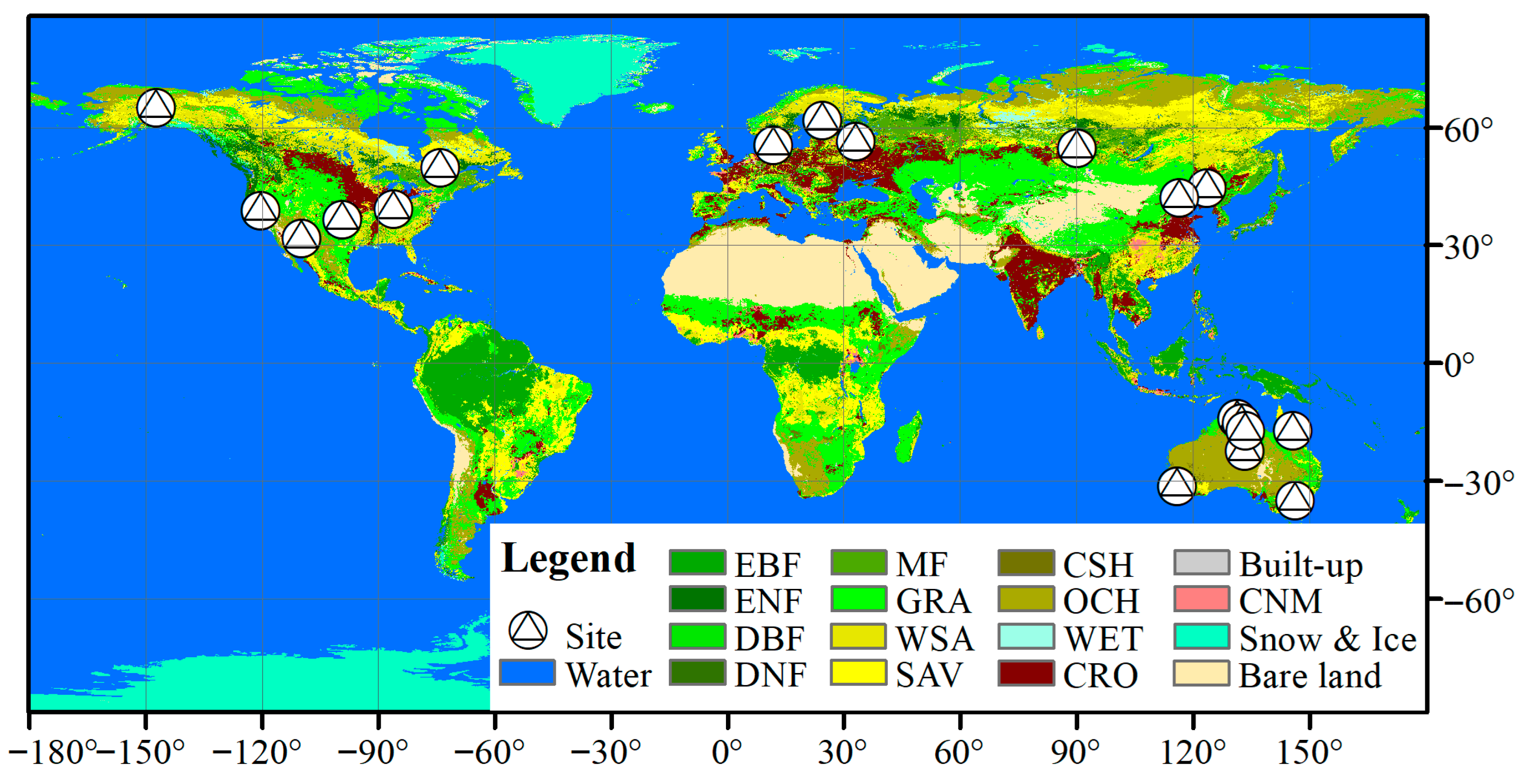
Figure 1. The spatial distribution map of flux tower sites that are representative at the 0.1° grid.
Remotesensing 17 03429 g001
Figure 2. The effects of Ntree and Depthmax on the model (a), the importance of predictor variables (b), the relationship between test SIFtotal and predicted SIFtotal (c) and the residuals of predicted SIFtotal in the final model (d). The red dashed line in (c) represents the regression line of the scatter points.
Remotesensing 17 03429 g002
Figure 3. Relationship between SIFtotal_01 and FLUXNET2015 GPP for all 19 EC flux sites. The red dashed line represents the linear regression fit (GPP = 1.70 × SIF −0.77, R2 = 0.81, RMSE = 2.80). The background hexagons indicate the data density on a logarithmic scale. The red dashed line represents the regression line.
Remotesensing 17 03429 g003
Figure 4. Relationship between GPP and SIFtotal_01 across different land cover types. (a) EBF and DBF, (b) Evergreen Needleleaf Forests (ENF), (c) GRA and OSH, and (d) WSA and SAV. The color gradient represents the logarithmic scale of data point density. The red dashed lines indicate the best-fit linear regression lines for each ecosystem type. The red dashed line represents the regression line.
Remotesensing 17 03429 g004
Figure 5. Temporal dynamics and diurnal correlations of GPP and SIF in the Haibei Steppe EC flux site. (a) Normalized time series of GPP, SIFz, and SIFtotal_01 in the daytime from June to August in 2019 and 2020. (be) Scatter plots showing relationships between normalized GPP and normalized SIF (SIFz in (b,d)), SIFtotal_01 in (c,e) during morning (b,c) and afternoon (d,e) periods. A black dot represents the average data for a specific hour within a month. The black solid line represents the regression line.
Remotesensing 17 03429 g005
Figure 6. Diurnal variation in normalized slope for all 19 EC flux sites with statistical comparisons between morning and afternoon periods. The black line with open circles shows the hourly normalized slope (mean ± SD) from 6:00 to 18:00. Gray shading denotes transitional periods at the beginning (6–7 h) and end (17–18 h) of the day. Red and blue dashed (and dotted) lines, together with corresponding labels, represent mean values and CV for the morning (AM, 6:00–12:00 or 7:00–12:00) and afternoon (PM, 12:00–18:00 or 12:00–17:00) periods, respectively. CVAM+PM denotes the overall CV for the combined daytime period.
Remotesensing 17 03429 g006
Figure 7. Diurnal variation in normalized slope for four different land cover groups with statistical comparisons between morning and afternoon periods. (a) EBF and DBF, (b) ENF, (c) GRA and OSH, and (d) WSA and SAV. The description of this figure is consistent with that of Figure 6.
Remotesensing 17 03429 g007
Figure 8. Global maps of estimated hourly SIFtotal_01 at 11:00–12:00 local solar time averaged over July 2008. In addition, fingerprints for selected flux tower sites are used to visualize hourly SIFtotal_01 (top) and GPP (bottom) for each month of 2008.
Remotesensing 17 03429 g008
Figure 9. Spatial maps of the difference of SIFtotal_01, APAR, and ΦSIF between morning and afternoon (ΔSIFtotal_01 = SIFtotal_01PM −SIFtotal_01AM, ΔAPAR = APARPM −APARAM, and ΔΦSIF = ΦSIFPM −ΦSIFAM) in July averaged over driest (a,c,e) and wettest (b,d,f) years for the period 2000–2022 in the MHNH region. For each pixel, the driest and wettest years were set as the years with the lowest and highest ERA5 SMmean from 2000 to 2022.
Remotesensing 17 03429 g009
Table 1. Statistical comparison of the relationships between GPP and different SIF products (SIFtotal_01 and SIFtotal) across different IGBP vegetation types.
ComparisonMSEMAERMSER2SlopeIntercept
GPP v.s. SIFtotal_01
in all IGBP types
7.812.112.80.821.7−0.77
EBF and DEF3.091.431.760.891.6−3.88
ENF5.211.762.280.841.85−0.07
GRA and OSH2.71.191.640.661.2−0.46
WSA and SAV10.462.583.230.481.59−0.12
GPP v.s. SIFtotal
in all IGBP types
8.322.242.890.811.81−0.97
EBF and DEF5.391.962.320.81.42−1.53
ENF51.772.240.841.880.01
GRA and OSH3.051.311.750.641.27−0.73
WSA and SAV10.842.653.290.461.580.28
Disclaimer/Publisher’s Note: The statements, opinions and data contained in all publications are solely those of the individual author(s) and contributor(s) and not of MDPI and/or the editor(s). MDPI and/or the editor(s) disclaim responsibility for any injury to people or property resulting from any ideas, methods, instructions or products referred to in the content.