Article

Assessment of the Effectiveness of Spectral Indices Derived from EnMAP Hyperspectral Imageries Using Machine Learning and Deep Learning Models for Winter Wheat Yield Prediction

1
Department of Atmospheric and Geospatial Data Science, University of Szeged, Egyetem Str. 2, H-6722 Szeged, Hungary
2
Lajtamag Ltd., Bereki Str. 1, H-9246 Mosonmagyaróvár, Hungary
3
Nemzeti Ménesbirtok és Tangazdaság Zrt., Jung József Sq. 1, H-5820 Mezőhegyes, Hungary
4
Laboratory for Climatology and Remote Sensing, Department of Geography, Philipps-Universität Marburg, Deutschhausstr. 12, 35032 Marburg, Germany
5
Department of Geology, Faculty of Science, Cairo University, Giza P.O. Box 12613, Egypt
6
Doctoral School of Geosciences, University of Szeged, Egyetem Str. 2, H-6722 Szeged, Hungary
*
Author to whom correspondence should be addressed.
Remote Sens. 2025, 17(20), 3426; https://doi.org/10.3390/rs17203426
Submission received: 11 August 2025 / Revised: 21 September 2025 / Accepted: 8 October 2025 / Published: 13 October 2025

Abstract

Highlights

What are the main findings?
  • Multi-temporal EnMAP hyperspectral data combined with machine learning and deep learning models significantly improved the accuracy of winter wheat yield prediction (R2 up to 0.79).
  • SWIR indices were particularly important for early-season estimation, whereas VNIR indices became dominant during later growth stages.
What are the implications of the main findings?
  • Integrating hyperspectral observations across phenological stages enables more robust and reliable yield forecasts for precision agriculture.
  • Future missions, such as ESA’s CHIME, will further enhance large-scale, operational crop yield monitoring by providing frequent, high-resolution hyperspectral data.

Abstract

Accurate and timely crop yield estimation is essential for effective agricultural management and global food security, particularly for winter wheat. This study aimed to assess the effectiveness of EnMAP hyperspectral imagery in combination with machine learning and deep learning models for winter wheat yield prediction in Hungary. Using EnMAP images from February and May 2023, along with ground truth yield data from four fields, we derived 10 distinct vegetation indices. Random Forest, Gradient Boosting, and Multilayer Perceptron algorithms were employed, and model performance was evaluated using Mean Absolute Error (MAE) and Coefficient of Determination (R2) values. The results consistently demonstrated that integrating multi-temporal data significantly enhanced predictive accuracy, with the MLP model achieving an R2 of 0.79 and an MAE of 0.27, notably outperforming single-date predictions. Shortwave infrared (SWIR) indices were particularly critical for early-season yield estimations. This research highlights the substantial potential of hyperspectral data and advanced machine learning techniques in precision agriculture, emphasizing the promising role of future missions such as CHIME in further refining and expanding yield estimation capabilities.

1. Introduction

Accurate and timely crop yield estimation is critical for agricultural management and global food security, especially for staple crops such as winter wheat [1,2]. Traditional methods are often costly and spatially limited, making advanced remote sensing technologies essential for non-invasive crop monitoring. The field has evolved from multispectral to hyperspectral imaging, with hyperspectral sensors offering superior detail through hundreds of contiguous, narrow spectral bands [3,4]. This fine resolution allows for the detection of subtle biophysical changes, which are crucial for assessing crop health and predicting yield [5,6,7].
In recent decades, significant advancements in crop yield prediction have been achieved using remote sensing and spectral vegetation indices, which are vital for precision agriculture [8,9]. Indices such as the NDVI and EVI, alongside red-edge-based indices, are widely used to quantify plant physiological status, with their temporal trajectories serving as reliable yield predictors for major crops [10,11]. Machine learning (e.g., Random Forest (RF), Gradient Boosting (GB)) and deep learning (e.g., CNN, LSTM) algorithms effectively capture nonlinear relationships in high-dimensional satellite data [12,13,14]. The efficacy of these models is significantly enhanced by higher spatial and temporal data resolution, with a growing trend towards SAR–optical fusion for improved biomass estimation, even under cloudy conditions [14,15]. Recent advancements also integrate hyperspectral data, time series analysis, and AI-based preprocessing for pixel-level yield prediction [16,17].
Launched in 2022, the Environmental Mapping and Analysis Program (EnMAP) is a pivotal German experimental hyperspectral mission that acquired 224 contiguous spectral bands from 400 nm to 2450 nm at a 30 m spatial resolution [3,18]. As a demonstration mission, EnMAP’s imagery availability is currently limited, posing a challenge for continuous, large-scale agricultural monitoring [19]. However, the upcoming European Space Agency’s (ESA) Copernicus Hyperspectral Imaging Mission for the Environment (CHIME), slated for 2028–2030, is expected to provide systematic global hyperspectral observations with more frequent revisit times, overcoming current issues relating to data scarcity and enabling more dependable multi-temporal yield estimation [20].
Given the complexity of hyperspectral data, machine and deep learning algorithms such as RF, GB, and CNN are well-suited to model the nonlinear relationships between spectral responses and crop yield [21,22,23,24]. At the same time, rapid advances in machine learning and deep learning have transformed the analysis of high-dimensional remote sensing datasets. Traditional regression models, while valuable, often struggle with the nonlinearities and collinearity inherent in hyperspectral and multi-temporal data. In contrast, ensemble learning methods such as RF and GB have been widely adopted for crop modeling because of their resilience to overfitting, ability to handle large predictor spaces, and strong predictive accuracy across diverse environmental conditions [21]. These algorithms have already shown promise for vegetation studies, biophysical parameter retrieval, and yield estimation.
In parallel, neural network-based methods, including Multilayer Perceptron (MLP) and more advanced deep architectures, have emerged as powerful alternatives for remote sensing data exploitation. Neural networks can learn hierarchical and nonlinear feature representations directly from raw or minimally processed input data, making them particularly suitable for complex spectral–temporal information. Deep learning approaches such as convolutional and recurrent neural networks have been successfully applied to tasks including land cover classification, biomass estimation, and crop yield forecasting [25]. However, despite this promise, their application to spaceborne hyperspectral datasets—particularly EnMAP’s unique multi-temporal data streams—remains relatively underexplored. This gap provides a valuable opportunity to evaluate the comparative performance of classical ensemble learners and neural networks in the context of winter wheat yield prediction.
Another critical aspect of crop yield modeling is the integration of multi-temporal information. Yield formation is inherently dynamic, reflecting processes that unfold from emergence to maturity. Single-date imagery often fails to capture the complexity of these temporal dynamics, whereas multi-temporal hyperspectral data enable the monitoring of growth trajectories, stress responses, and phenological transitions. By exploiting EnMAP’s revisit cycle, researchers can identify the most informative time windows for yield prediction and design models that incorporate cumulative effects of environmental conditions across the growing season. Recent studies using multispectral data have demonstrated the value of temporal information; for example, Peng et al. [26] combined Sentinel-2 and weather forecast data with deep learning (PyTorch 3.8) to improve in-season yield prediction of winter wheat in China, while Li et al. [27] fused convolutional neural networks with multi-attention LSTMs to capture temporal dependencies in crop growth. Similar approaches using hyperspectral multi-temporal data, such as those provided by EnMAP, are expected to further enhance prediction accuracy and generalizability.
The present study systematically evaluates the potential of spaceborne hyperspectral remote sensing for winter wheat yield prediction by exploiting multi-temporal EnMAP data and comparing the performance of state-of-the-art ML and DL algorithms. Specifically, we assess the predictive capacity of RF regression (RFR), GB regression, and MLP neural networks using spectral–temporal features derived from EnMAP imagery across key phenological stages. By benchmarking these approaches against one another, we aim to identify both the strengths and limitations of classical ensemble learners and neural networks when applied to operational hyperspectral data.
The present study builds upon a series of prior investigations by the authors that focused on crop yield estimation using multisource satellite data and advanced machine learning and deep learning techniques. Our previous works [28,29,30,31] demonstrated the potential of combining high-resolution satellite imagery (e.g., PlanetScope, Sentinel-2, Landsat 8, and DESIS) with environmental and topographic data for improving within-field yield estimation and crop type classification (ERDAS IMAGINE 2020, QGIS 3.16, Python 3.10). These studies explored various methodological approaches, including data fusion techniques, vegetation index time series, and machine learning algorithms, such as Random Forest and deep neural networks, to predict soybean and wheat yields with high accuracy. The findings highlighted the value of integrating satellite imagery with ancillary data and the effectiveness of fusion-based and hyperspectral approaches in enhancing yield predictions. The current research extends this body of work by further refining the models and applying them in a new context, thus contributing to the ongoing efforts in precision agriculture and remote sensing-based crop monitoring.
The main goal of this study is to evaluate the efficacy of EnMAP hyperspectral imagery combined with machine learning and deep learning regression models for winter wheat yield estimation in Hungary. A key focus of this investigation is to determine how the broader spectral range of single and multiple EnMAP imageries—particularly through the application of SWIR indices—contributes to yield estimation. This research lays the groundwork for future applications with more abundant hyperspectral data from missions such as CHIME, which is expected to have parameters similar to EnMAP [20].

2. Materials and Methods

2.1. Study Area

The study area, as shown in Figure 1, is located in southeastern Hungary, near the Romanian border, within the administrative boundaries of Mezőhegyes, Békés County (46°19′N, 20°49′E). Mezőhegyes encompasses approximately 15,544 hectares (ha) and has a population of around 4950. The region is characterized by fertile chernozem soils, particularly in its meadow and lowland areas, which are rich in calcium carbonate and highly suitable for cultivating cereals and oilseeds. The area is home to Nemzeti Ménesbirtok és Tangazdaság Zrt., a major agricultural enterprise operating on nearly 9862 hectares, which also influences agricultural activity in neighboring settlements. For this study, four agricultural fields within the area were selected. Each field was sown with winter wheat in 2023.
All four agricultural plots shown in Figure 1 were sown with the winter wheat variety Avenue in 2023, using a no-tillage cultivation system. Importantly, all plots were fertilized 7–10 days after sowing, and no additional fertilization was applied in spring. Furthermore, the same agricultural treatments were applied across the fields, including foliar fungicides, stem-strengthening agents, and fungicidal applications during heading. The first plot (Figure 1) covers an area of 33.74 ha, with a field-level yield of 7.63 t/ha in 2023. The second plot spans 115 hectares and produced 5.97 t/ha. The third plot measures 56.5 hectares, with a yield of 6.95 t/ha, while the fourth plot covers 63 hectares and yields 6.38 t/ha.

2.2. Cultivar Characteristics

Avenue is a medium-maturing winter wheat cultivar (Triticum aestivum L.) suitable for both conventional and high-input farming systems. Originally bred in Western Europe, it has become increasingly widespread across Central and Eastern Europe in recent years [32,33]. The variety shows strong adaptability to continental climatic conditions, supported by its reliable winter hardiness and balanced vernalization requirements. With a medium plant height (85–95 cm) and sturdy stem strength, Avenue exhibits good lodging resistance, making it well-suited for intensive management [32]. One of its key agronomic traits is its excellent tillering capacity, which promotes rapid early canopy development, favoring biomass accumulation and efficient nutrient uptake during the initial growth period [6]. The cultivar demonstrates high resistance to powdery mildew (Blumeria graminis) and yellow rust (Puccinia striiformis), along with moderate tolerance to other foliar diseases [7,33]. Phenologically, the cultivar typically reaches heading in early May (BBCH 51–59), followed by a short flowering phase, aligning well with Central European harvesting calendars [34]. Its grain quality is consistently good, and under adequate nitrogen management, it can reach milling standards, characterized by medium to high protein content and stable gluten performance [35]. Overall, Avenue offers a favorable combination of yield potential, disease resistance, and agronomic flexibility, making it a reliable option under variable climatic and market conditions.

2.3. Study Period and Phenological Context

2.3.1. Agro–Climatic Conditions During the 2023 Growing Season

In the 2023 growing season, the phenological development of winter wheat (Triticum aestivum L.) was significantly influenced by drought at sowing, which strongly affected the spectral characteristics observable via remote sensing. During sowing (October 2022), monthly precipitation was minimal (11.7 mm), indicating suboptimal starting conditions. Moderate rainfall in winter—especially in December and January (58.4 mm and 51.5 mm in monthly totals)—partially restored soil moisture. February saw relatively dry conditions (18.5 mm in monthly total) at the onset of spring regrowth. In contrast, May recorded the highest precipitation (96.5 mm in monthly total), which likely benefited flowering and grain filling. These trends demonstrate that crop development depended not only on the satellite observation dates but also on overall precipitation distribution throughout the period.
At sowing time (October 2022), the average temperature of 13.3 °C provided favorable conditions for early crop growth. During the winter months, temperatures gradually declined, reaching 2.84 °C in February, marking the crop’s dormancy phase. From March onward, rising temperatures (peaking at 15.92 °C in May) supported active spring development, including stem elongation, heading, and flowering.
The February and May satellite images thus captured two distinct growth stages (tillering and heading), and understanding this temperature dynamic is important for interpreting spectral indices and improving yield estimation accuracy.

2.3.2. Phenological Development and Spectral Characteristics in 2023

In February, corresponding to the end of tillering and the onset of stem elongation (BBCH 29–31), the weather was characterized by cooler and wetter weather than average, resulting in increased spatial heterogeneity of plant development. This heterogeneity was reflected in the spectral variance, particularly in the red-edge and near-infrared (NIR) bands, which are sensitive to changes in chlorophyll content and the leaf area index (LAI) [6,34]. On the NDVI time series, it can be clearly observed that in February, the values of the vegetation indices gradually increased as the wheat emerged from its winter dormancy and growth became more intense. This upward trend continued towards the May period, indicating rapid biomass accumulation and canopy closure. By May, during the heading (BBCH 51–59) and flowering (BBCH 60–69) stages, the canopy reached its maximum biomass and photosynthetic activity, leading to more stable spectral signatures, which typically results in a plateau in NDVI values (Figure 2). These later phenological stages provided optimal conditions for yield prediction models, especially when using hyperspectral data [7,23]. Recent studies confirm that early-season hyperspectral observations, such as those from February, can already offer relevant predictive information; however, data acquisition in May remains superior in their predictive accuracy due to the phenological maturity and spectral stability of the crop [2,16]. Therefore, precise timing and data acquisition timed to crop phenology were found to be crucial for pixel-level yield estimation in 2023, even under the year’s challenging agro–climatic conditions [19].

2.4. Preprocessing of the Study Fields and Yield Data

Hyperspectral Dataset

The EnMAP hyperspectral sensor was designed to monitor and analyze Earth’s surface with high spectral fidelity [3,36]. EnMAP provides hyperspectral imagery in the visible, near-infrared (VNIR: 420–1000 nm), and shortwave infrared (SWIR: 900–2450 nm) regions, capturing data in a total of 224 contiguous spectral bands [36,37]. The satellite offers a spatial resolution of 30 m and a swath width of approximately 30 km, making it well-suited for large-scale environmental and land surface monitoring [38].
EnMAP’s high spectral resolution allows for the discrimination of subtle differences in surface materials, vegetation types, and land cover characteristics [4]. EnMAP’s data are particularly valuable for applications in agriculture, forestry, geology, water quality assessment, and urban studies [18,39]. The imagery used in this study was atmospherically corrected and georeferenced, enabling accurate integration with ground-based and ancillary geospatial datasets for advanced modeling and analysis [3].
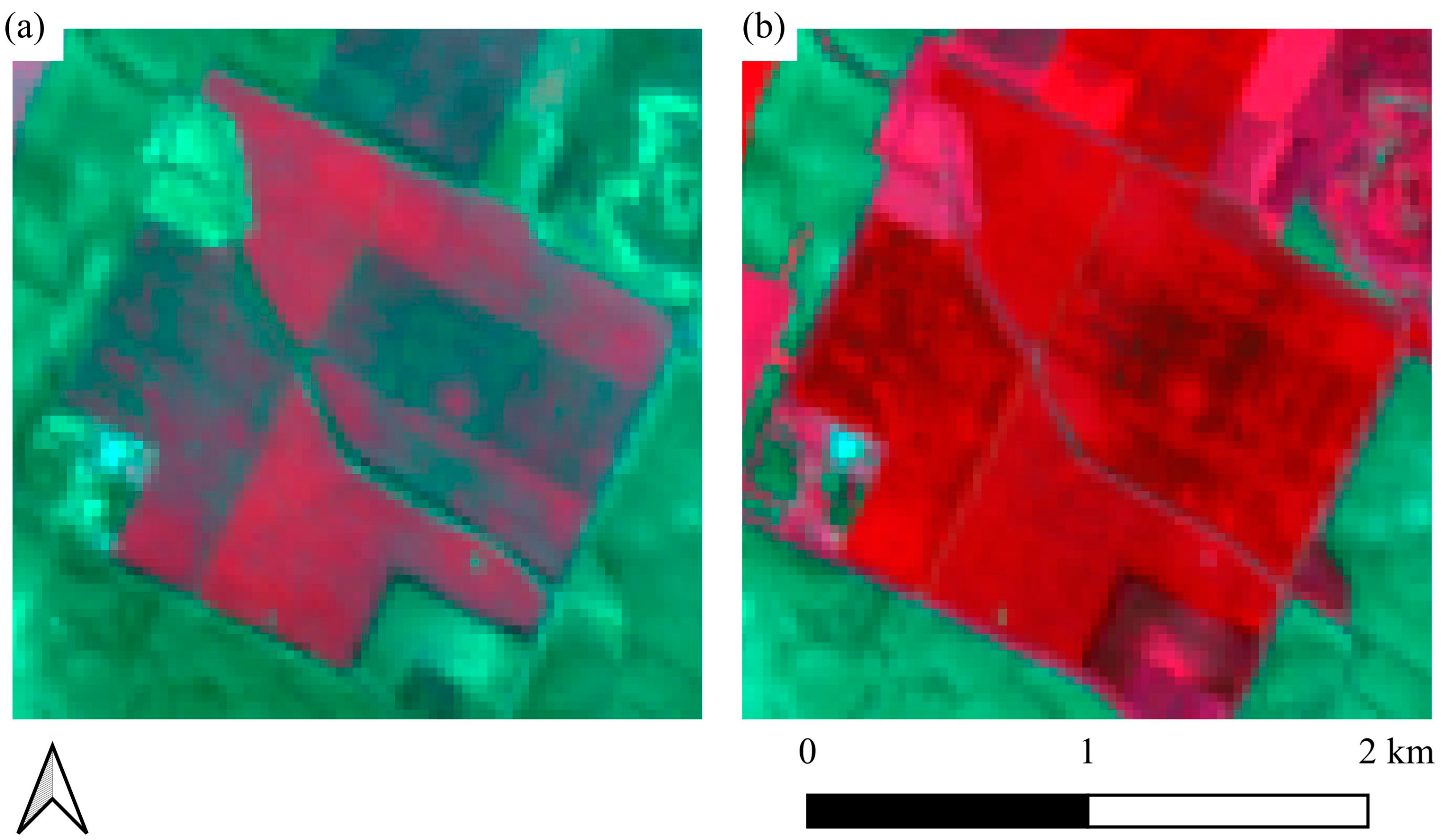
In the research, four agricultural parcels were selected within the study area. Each of these fields was cultivated with winter wheat in 2023. Satellite imagery was acquired on 23 February and 8 May 2023 (Figure 3). To ensure spatial alignment, the two images were geometrically co-registered with each other using ground control points and image-matching techniques.

2.5. Yield Data

The analyzed pixels were selected based on a buffer applied to the parcel boundaries. This buffer was used to exclude edge areas where spectrally mixed pixels are more likely to occur. Only the pixels fully enclosed within the buffered parcels were considered in the analysis to ensure data homogeneity and accuracy. Yield data for the 2023 season were provided by Nemzeti Ménesbirtok és Tangazdaság Zrt., based on measurements obtained using precision agricultural combine harvesters. Prior to analysis, the raw yield data were cleaned to remove outliers and inconsistencies, and values were capped at 11 tons per hectare to remove extreme outliers and non-representative measurements, and to facilitate consistent comparison across the parcels. Following the data cleaning and normalization process, the yield point data were spatially aggregated to match the resolution and grid structure of the hyperspectral satellite imagery. Specifically, yield measurements were aggregated within each pixel-sized grid cell defined by the satellite imagery. On average, each cell contained 68 measurements, and their mean value was used to represent the cell’s yield. This rasterization step ensured that the ground-based yield values were spatially aligned with the satellite-derived data on a per-pixel basis, enabling direct pixel-wise comparison and subsequent modeling. The result was a gridded yield dataset with the same spatial geometry as the hyperspectral imagery, facilitating accurate integration of ground truth and remote sensing observations.
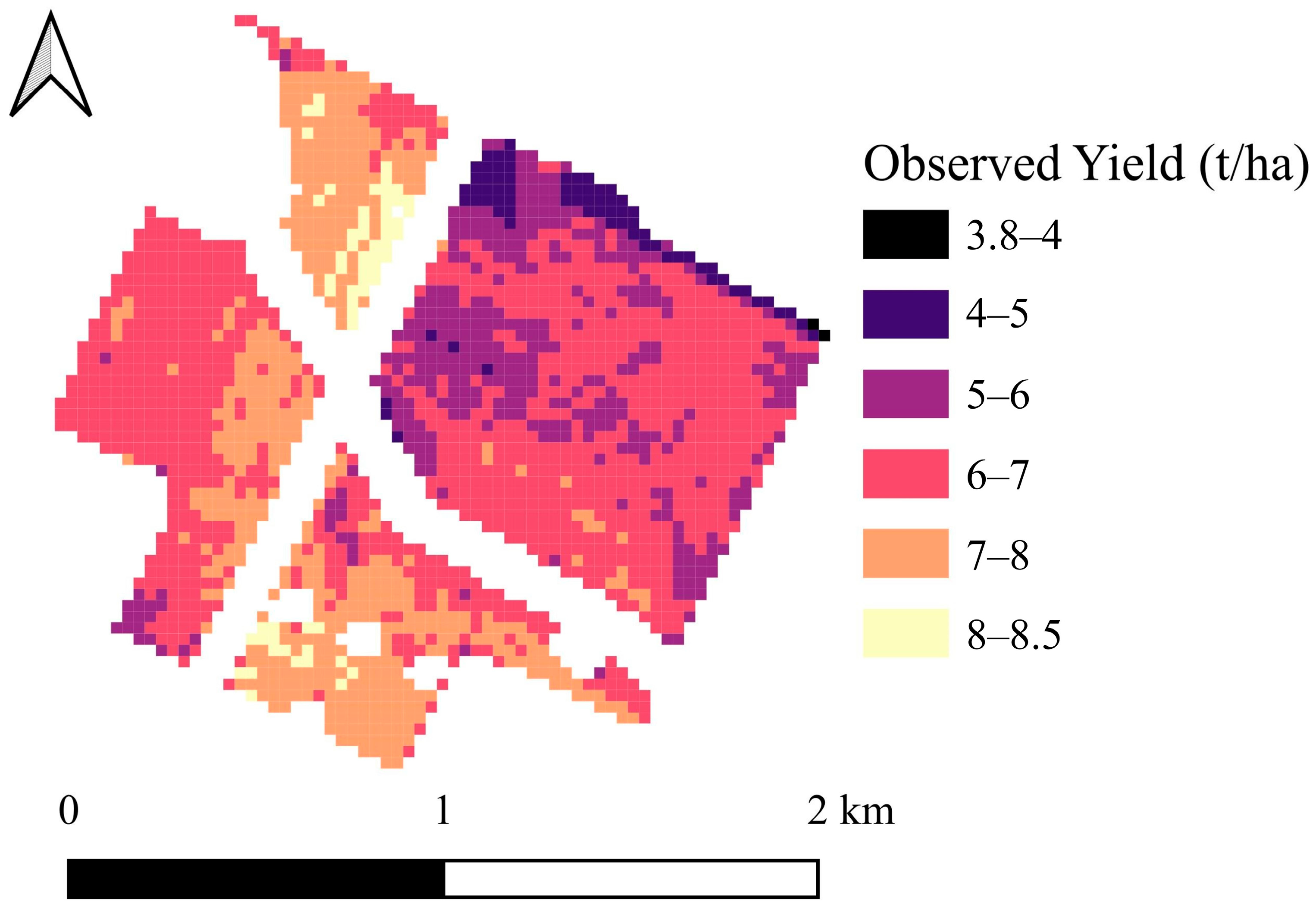
The observed yield values ranged between 3.8 and 8.5 t/ha, with variability between the individual fields reflecting differences in soil conditions, management practices, and microclimatic factors. The study area includes four agricultural fields of varying sizes and yield data densities. Following data cleaning and filtering, the first field covers an area of 21.35 ha, with approximately 16,700 yield measurement points. The second field spans 94.57 hectares and contains around 67,200 points. The third field covers 34.4 hectares with about 25,800 points, while the fourth field encompasses 45.58 hectares, with roughly 37,900 yield measurements (Figure 4).

2.6. Spectral Characteristics of Yield Extremes

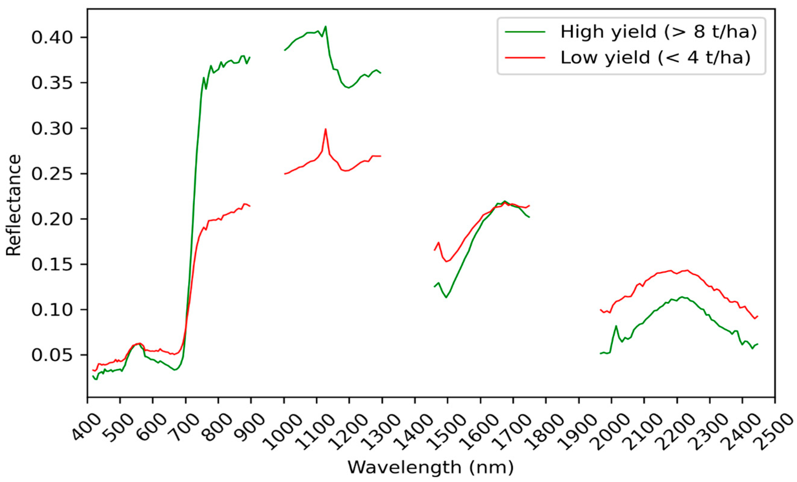
The spectral reflectance curves from the EnMAP acquisition in February (Figure 5) reveal distinct differences between low (<4 t/ha) and high (>8 t/ha) yield winter wheat pixels, providing early insights into potential yield variations. Notably, the high-yield pixels consistently exhibit significantly higher reflectance in the NIR region (approx. 700–1300 nm) compared with their low-yield counterparts. This pronounced difference in NIR reflectance in early February is indicative of healthier, more vigorous vegetation with a greater biomass accumulation and/or higher plant density, reflecting superior cellular structure and overall plant vitality after the winter period. While subtle variations are also observable in the visible spectrum, where high-yield areas show slightly lower red and higher green reflectance, suggesting improved chlorophyll content, the strong divergence in the NIR band serves as an essential early-season indicator of the crop’s condition and its future yield potential, which is highly valuable for remote sensing-based yield forecasting.
The May spectral reflectance curves for winter wheat pixels exhibit strong differentiation between high (>8 t/ha) and low (<4 t/ha) yield areas during a critical growth stage (Figure 6). High-yield pixels show notably lower reflectance in the red visible spectrum and significantly higher reflectance across the NIR. This significant divergence in the NIR band directly indicates healthier biomass accumulation, higher LAI, and a more vigorous canopy structure in the high-yielding fields. Furthermore, slight differences in the SWIR region related to water content and dry matter further support the characterization of healthier, more productive plant stands. These pronounced spectral distinctions in May provide key data for precise in-season yield estimation.

2.7. Calculation of Vegetation Indices

Vegetation-related spectral indices were derived using the Spectral Index Creator toolbox within the EnMAP-Box 3 plugin in QGIS. In total, 10 vegetation indices were selected for further analysis, based on their correlation with observed yield values and their representation of key physiological and structural vegetation traits. At least one index was chosen from each of the major spectral indicator categories: Structural characteristics, chlorophyll content, carotenoids and anthocyanins, leaf water content, and dry matter. This selection ensured a comprehensive description of crop biophysical status relevant to yield estimation. During the selection process, we aimed to include indices incorporating reflectance in the SWIR region, as these are particularly sensitive to water and dry matter content, which are important for yield prediction. All possible VNIR and SWIR indices were generated from the EnMAP-Box, and the regression models were run for each index individually. Only those indices that achieved an R2 value of at least 0.2–0.3 were selected for further analysis. From the selected indices, we identified those whose exclusion did not affect or even improved the model’s performance. While redundant input VI layers were present, omitting them would have significantly reduced the model’s predictive accuracy. This process ensured that the selected indices provided optimal performance for the yield prediction models, capturing the most relevant biophysical characteristics without introducing unnecessary complexity.
The Anthocyanin Reflectance Index 1 (ARI1) is sensitive to anthocyanin concentration in vegetation, which is often associated with plant stress, senescence, or nutrient deficiency. The ARI1 is particularly useful in detecting early stress signals in crops; it uses reflectance in the red (around 550 nm) and near-infrared (around 700 nm) regions (Table 1). Increased anthocyanin content leads to higher absorption in the green and red regions, which the ARI1 captures effectively [5].
The Hyperspectral NDVI (hNDVI) extends the traditional NDVI by dynamically selecting optimal narrow red (around 670–680 nm) and NIR (750–800 nm) wavelengths from hyperspectral data, improving sensitivity to vegetation chlorophyll content and reducing saturation in dense canopies [40].
The Carotenoid Reflectance Index 2 (CRI2) is a spectral index sensitive to carotenoid pigment content in vegetation, which plays a crucial role in photoprotection and stress responses. The CRI2 is calculated using reflectance values typically around 510 nm and 550 nm wavelengths, capturing variations in carotenoid concentration that often indicate plant stress or senescence. This index is useful for early detection of vegetation health and stress status in precision agriculture and ecological monitoring [41].
The Transformed Chlorophyll Absorption in Reflectance Index (TCARI) is designed to minimize the influence of leaf background and soil reflectance effects, focusing on chlorophyll content in vegetation. The TCARI uses reflectance bands around 670 nm, 700 nm, and 550 nm to better isolate chlorophyll absorption features, improving sensitivity especially in areas with sparse vegetation or mixed backgrounds [42].
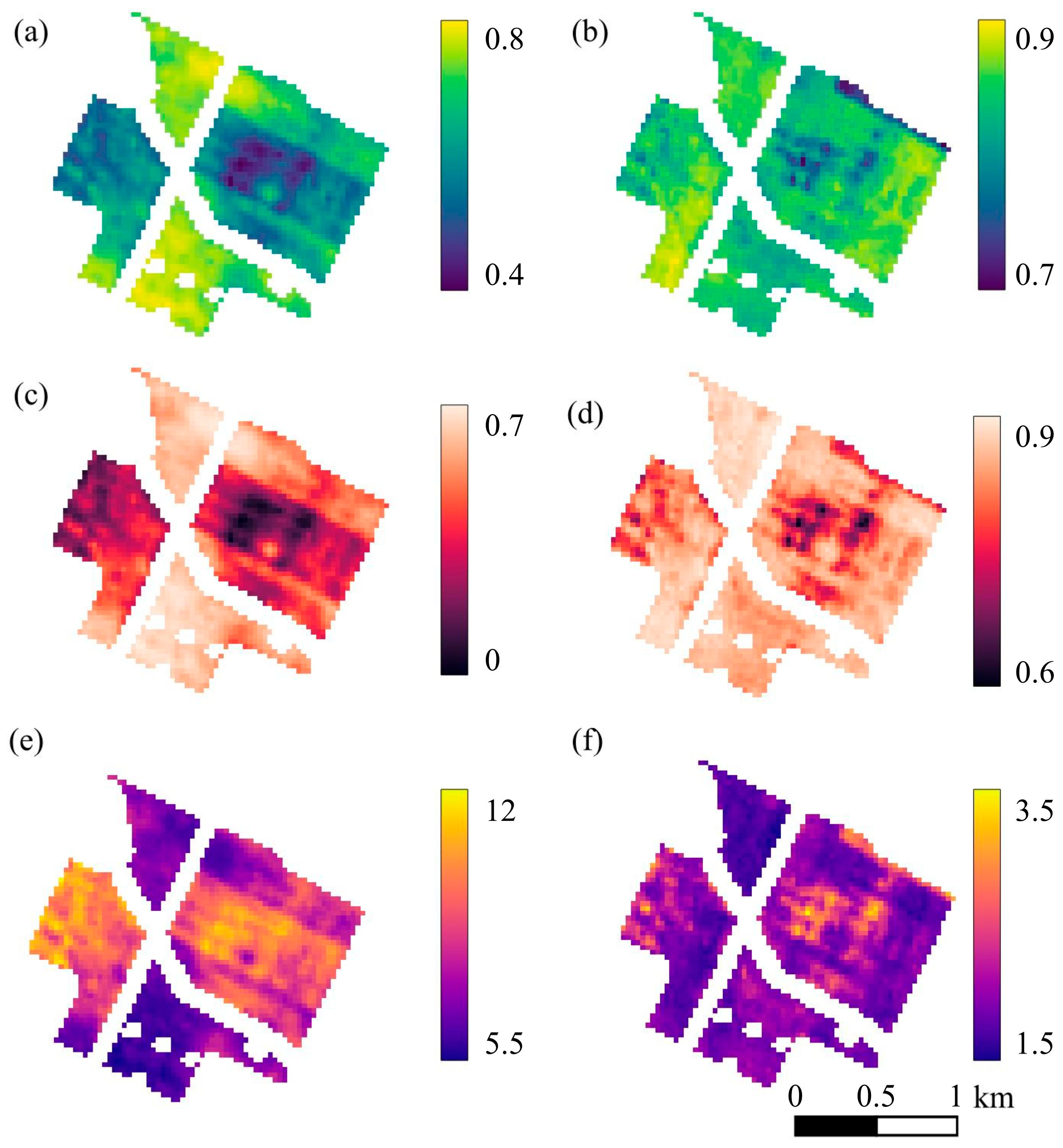
The Green Normalized Difference Vegetation Index (gNDVI) is a vegetation index similar to the traditional NDVI but uses the green spectral band instead of the red band to better capture variations in chlorophyll content and plant health. By comparing reflectance in the green (~550 nm) and near-infrared (~800 nm) regions, the gNDVI can be more sensitive to early stress detection and subtle changes in canopy structure, especially in dense vegetation. This makes it particularly useful for precision agriculture and monitoring crop vigor [43] (Figure 7).
The Transformed Vegetation Index (TVI) is a nonlinear modification of the NDVI that is calculated as the square root of (NDVI + 0.5). This transformation helps reduce the saturation effect common in the NDVI under dense vegetation and improves sensitivity in areas with medium biomass. The TVI has been shown to better separate vegetated and non-vegetated areas, particularly during periods of active growth. In this study, the TVI was included in the May dataset, when vegetation cover was more developed and traditional indices such as the NDVI may become less effective due to signal saturation [44].
The Two-band Enhanced Vegetation Index (EVI2) is an improved vegetation index developed to overcome some limitations of the NDVI, such as saturation in dense vegetation areas and sensitivity to soil background and atmospheric effects [45].
The Global Vegetation Moisture Index (GVMI) is used to estimate vegetation water content by combining reflectance in the near-infrared (around 860 nm) and shortwave infrared (around 1240 nm) bands (Table 2). The GVMI is sensitive to changes in leaf moisture and can indicate plant water stress, making it valuable for drought monitoring and precision agriculture applications [5] (Figure 7).
The Moisture Stress Index (MSI) is designed to detect moisture stress in vegetation by comparing reflectance in the NIR and SWIR regions. The MDI is calculated using bands around 820 nm (NIR) and 1600 nm (SWIR). An increase in MSI values generally indicates a reduction in leaf water content, making it a reliable indicator of drought stress or irrigation deficiency in crops [5].
The Normalized Difference Water Index (NDWI) is used to monitor vegetation water content and soil moisture by comparing reflectance in the green (~860 nm) and near-infrared (~1240 nm) spectral bands. Higher NDWI values indicate greater water content, making it especially useful for early detection of plant water stress and drought conditions [46].
The Shortwave Infrared Vegetation Index (SWIRVI) utilizes reflectance in specific shortwave infrared wavelengths to provide detailed insights into vegetation structure and water content. By focusing on bands around 2090 nm, 2208 nm, and 2210 nm, the SWIRVI is particularly sensitive to biomass and moisture variations, making it an effective tool for precision agriculture and monitoring vegetation stress [1] (Figure 7).

2.8. Model Training

In this study, crop yield estimation was performed using the Forest-based Classification and Regression tool available in ArcGIS Pro. This tool implements two ensemble learning algorithms, RF and GB, both of which are based on decision tree structures. The RF algorithm creates multiple decision trees using random subsets of the training data and input variables (bagging) and aggregates their outputs to improve accuracy and reduce overfitting. In contrast, GB builds trees sequentially, where each tree attempts to correct the residual errors of the previous ones, enhancing model performance in complex data environments. These methods are well-suited for remote sensing applications due to their ability to handle nonlinear relationships, high-dimensional input (such as multispectral or hyperspectral data), and missing values, while also providing interpretable feature importance scores.
In the training process, both the Random Forest and Gradient Boosting models were configured with 500 trees to ensure consistency in ensemble size (Table 3). However, their internal tree structures differed to reflect the unique learning strategies of each algorithm. For the Random Forest, we used a maximum tree depth of 15 and a minimum leaf size of 5, allowing for deeper, more granular splits that capture complex interactions in the feature space. In contrast, the Gradient Boosting model employed shallower trees with a maximum depth of 10 and a larger minimum leaf size of 10. This setup aimed to balance predictive power and regularization, minimizing overfitting while preserving model sensitivity to important spectral features.
In addition to tree-based ensembles, an MLP neural network was implemented to provide a complementary, non-tree-based perspective on yield prediction. The MLP was developed in Python 3.8 using the MLPRegressor implementation from the scikit-learn 0.24.2 library. The model was configured with three hidden layers of decreasing size (128, 64, and 32 neurons), each using rectified linear unit (ReLU) activation functions to capture nonlinear feature interactions (Table 3). The network was trained with the Adam optimizer, an initial learning rate of 0.001, and an L2 regularization term (α = 0.001) to improve generalization. A maximum of 500 iterations was allowed for convergence, with training driven by the minimization of mean squared error loss. To ensure reproducibility, a fixed random seed (42) was applied. This configuration provided a balance between model complexity and computational efficiency, enabling the MLP to approximate complex relationships in the input data while maintaining stability during training.

2.9. Validation

To ensure independence between training and validation, 30% to 50% of the samples were randomly withheld from the training data for validation purposes. This random partitioning was conducted separately within each of the four datasets. As a result, the validation pixels were completely excluded from the model training process, allowing for an unbiased evaluation of model performance on unseen data. Model performance was assessed using metrics including the Mean Absolute Error (MAE) and the Coefficient of Determination (R2), providing quantitative measures of prediction accuracy and goodness of fit.
The Mean Absolute Error (MAE) was calculated as follows:
M A E = 1 n i = 1 n y i y i ^
where n is the number of samples; yi is the observed (true) value; and y i ^ is the predicted value.
The Coefficient of Determination (R2) was calculated as follows:
R 2 = 1 i = 1 n y i y i ^ 2 i = 1 n y i y _ 2
where y _ = 1 n i = 1 n y i is the mean of the observed values.

2.10. Feature Importance

In this study, feature importance values were derived and compared across the RF, GB, and MLP models. For the ensemble tree-based algorithms (RF and GB), importance was quantified through impurity reduction and expressed as the mean decrease in variance contributed by each predictor variable across the trees. Since MLP does not inherently provide feature importance, we employed a permutation-based approach, where each predictor was randomly shuffled and the resulting decrease in model performance (R2, MAE) was recorded as an indicator of its relevance. To ensure comparability between the different modeling frameworks, all feature importance values were normalized to percentages summing to 100%. This consistent scaling enabled a direct evaluation of the relative contribution of explanatory variables across fundamentally different machine learning methods.

3. Results

3.1. Spectral Predictor Variables and Feature Importance

In this study, a wide range of indices derived from multiple EnMAP scenes was initially included in the training process for both acquisition dates. However, the use of several indices did not lead to performance improvements and, in some cases, even significantly reduced model accuracy. For the May acquisition, we ultimately identified a subset of relevant indices (10), although not all of them proved suitable for the February dataset (6). In the multi-temporal model, the indices selected for each acquisition date were combined into a unified feature set.
In the February dataset, the forest-based models (RF and GB) exhibited a clear preference for VIS indices, particularly the ARI1 (RF: 23%, GB: 22%) and gNDVI (RF: 20%, GB: 16%), which were the most influential predictors for crop yield (Figure 8). SWIR indices such as the SWIRVI (RF: 15%, GB: 19%), NDWI (RF: 13%, GB: 15%), MSI (RF: 14%, GB: 14%), and GVMI (RF: 16%, GB: 14%) also contributed, indicating that RF and GB integrate both vegetation greenness and water- or moisture-sensitive information. Random Forest relied more heavily on VIS/VNIR indices compared with SWIR, while Gradient Boosting showed a somewhat more balanced distribution across VIS/VNIR and SWIR indices, with the SWIRVI and NDWI gaining relatively higher importance (Figure 8).
In contrast, the MLP model displayed a markedly different pattern. The MLP model’s predictions were dominated by SWIR indices, with the NDWI (29%), MSI (22%), and SWIRVI (16%) contributing the largest shares, while VIS indices such as the ARI1 (6%) and gNDVI (21%) had comparatively minor influence. This suggests that MLP captures nonlinear relationships associated with water content and soil or crop moisture, rather than relying primarily on visible-range vegetation signals.
For the May acquisition, both the RF and GB single-date models identified a diverse set of important vegetation indices. In the RF model, the ARI1 (17%) and gNDVI (16%) were the most influential, while in the GB model, the gNDVI (18%) and SWIRVI (15%) ranked highest (Figure 9). Notably, indices based on SWIR bands (SWIRVI, MSI, GVMI, and NDWI) accounted for approximately 33% of the total relative importance in the RF model and about 37% in the GB model, highlighting that SWIR information remains important but slightly less dominant in May compared with February. Other influential indices, such as the TVI, hNDVI, and EVI2, reflect visible and near-infrared signals associated with pigment content and canopy structure (Figure 9).
In contrast, the MLP model showed a markedly different pattern. The MLP model’s predictions were dominated by SWIR indices, with the MSI (43%) and TVI (23%) contributing the largest shares, while VIS/VNIR indices such as the hNDVI (14%) and EVI2 (5%) had a lower influence. The other VIS/VNIR indices had negligible impact. This indicates that MLP emphasizes canopy moisture and water-related properties, capturing nonlinear relationships not fully exploited by the forest-based models.
Overall, while RF and GB integrate information from both VNIR and SWIR regions, ensuring a balance between chlorophyll- and moisture-sensitive features, MLP relies primarily on SWIR bands, reflecting a different spectral sensitivity. The comparison underscores the complementary strengths of forest-based and neural network approaches in estimating winter wheat yield during the mid-growing season.
In the multi-temporal models combining spectral indices from February and May, the distribution of feature importance shows notable differences across model types. For the RF model, indices derived from the May acquisition contributed approximately 59%, while February indices accounted for about 41%, indicating a stronger reliance on May data, with a slight bias towards early-season information. In contrast, the GB model placed slightly more emphasis on May data (57%) compared with February (43%) (Figure 10).
Among the most important features for both forest-based models were the ARI1 and gNDVI. In the RF model, the ARI1 (May, 14%) and gNDVI (May, 13%) were the top contributors, followed closely by the gNDVI (February, 11%) and ARI1 (February, 10%). For GB, the gNDVI (May, 12%) and ARI1 (February, 11%) ranked highest, highlighting minor differences in emphasis between model types. These indices are sensitive to chlorophyll and pigment content, with the ARI1 responsive to anthocyanin concentration and the GNDVI reflecting canopy greenness and nitrogen status.
SWIR indices contributed a significant fraction to both forest-based models, particularly in February. In RF, SWIR bands accounted for approximately 32% of total importance (February: 20%, May: 11%), while in GB, they represented around 35% (February: 21%, May: 14%), underscoring their relevance for water content and canopy moisture early in the season.
By contrast, the MLP model displayed a distinctly different pattern, with the VNIR index TVI (May, 33.6%) being the most important index, while the SWIR-sensitive MSI (February, 24%) also played a significant role in the predictions. In contrast, the remaining VIS indices had minimal influence. Indices such as ARI1 (May, 1.18%) and gNDVI (May, 3.31%), which were important in the forest-based models, proved to be completely negligible here. This indicates that MLP primarily captures nonlinear relationships associated with canopy moisture and water content, while still incorporating some visible-range information through the TVI, in contrast to the forest-based models, which balance information from both VIS/VNIR and SWIR indices to account for vegetation vigor and pigment content.
In summary, both forest-based multi-temporal data models highlight the dominance of VIS/VNIR indices related to chlorophyll, canopy structure, and pigment concentration, while also demonstrating that SWIR-based indices add meaningful predictive power, especially in early-season conditions. However, the MLP multi-temporal model relies to a lesser extent on most VIS indices, underlining differences in feature utilization across modeling approaches and the benefit of including a wide spectral range and multiple phenological stages in crop yield estimation workflows.

3.2. Yield Prediction Validation

The model validation was conducted under two data partitioning schemes: a 70% training and 30% validation split, and an equal 50–50% split. To ensure robustness and minimize the influence of random variation in the training–validation separation, each scenario was run five independent times. The performance metrics reported in this study represent the averaged results across these repetitions, providing a more reliable and stable assessment of model accuracy.
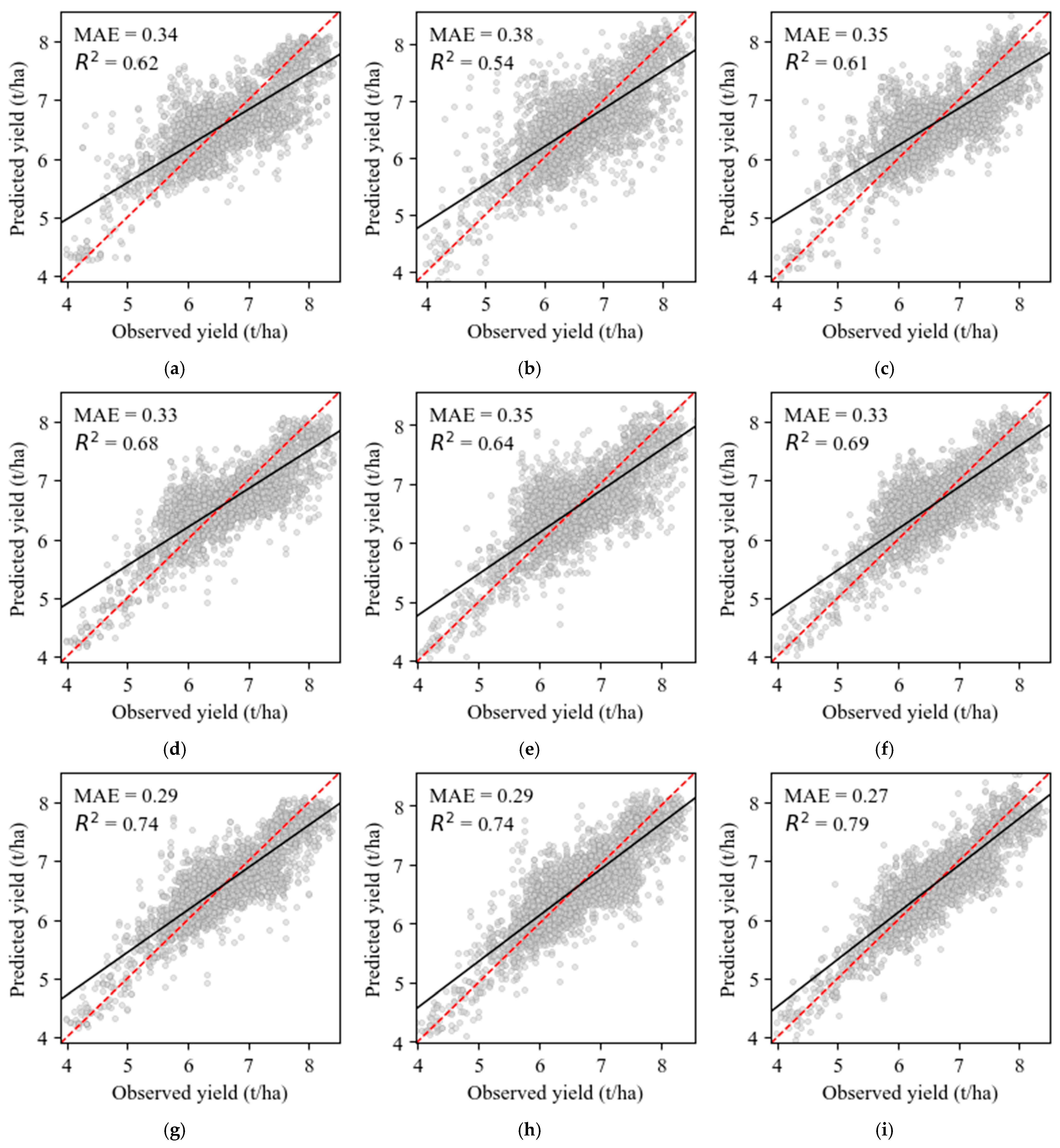
Figure 11 illustrates the performance of RF, GB, and MLP models for winter wheat yield prediction, where a 70% training and 30% validation split was employed for model development and evaluation. Across all temporal scenarios (February, May, and multi-temporal), the RF, GB, and MLP models exhibited comparable and robust predictive capabilities, with their respective MAE and R2 values remaining remarkably close. This suggests that for the given dataset and feature set, both ensemble learning approaches are similarly effective in modeling the complex, nonlinear relationships between spectral data and final yield.
Temporally, early-season predictions utilizing February indices yielded respectable performance (R2 ≈ 0.62, MAE ≈ 0.34), showing the value of crop vigor data captured even during early growth stages. Predictions based solely on May indices showed a marginal improvement (May GB: R2 = 0.69, MAE = 0.33), consistent with this period representing peak biomass and physiological activity. Significantly, the integration of both February and May spectral information into a multi-temporal framework resulted in a significant enhancement of predictive accuracy (R2 = 0.79, MAE = 0.27 for MLP; R2 = 0.74, MAE = 0.29 for both RF and GB). This improvement highlights the added benefit of capturing phenological development across distinct growth phases, providing a more comprehensive and reliable foundation for remote sensing-based yield forecasting by accounting for temporal dynamics in crop health and structure.
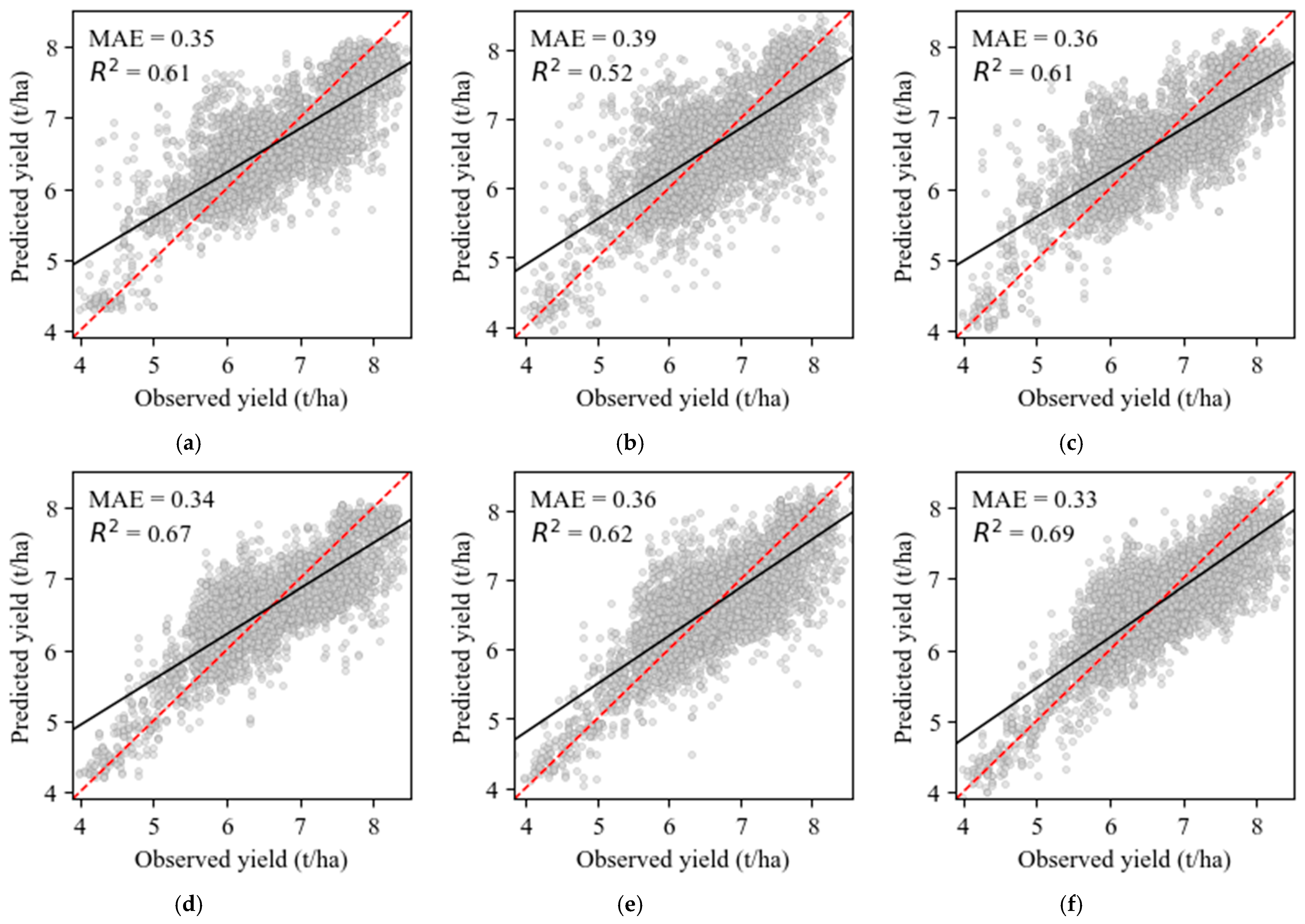
Figure 12 presents the winter wheat yield prediction performance of the RF, GB, and MLP models, evaluated using a more rigorous 50% training and 50% validation data split to better assess their potential real-world applicability. For single-date estimations, GB lagged behind RF and MLP, which achieved nearly identical results. However, with multi-temporal data, GB outperformed the other forest-based model, while MLP delivered the best performance overall (R2 = 0.79, MAE = 0.27), showing a clear advantage over the others. Notably, the MLP model produced virtually identical results under both the 70–30 and 50–50 data splits, highlighting its robustness to different training–validation partitions.
This consistent performance under a demanding 50% validation scenario strongly validates the practical utility of leveraging phenological development across distinct growth phases for precise and reliable remote sensing-based yield forecasting. Across all models and scenarios, a consistent bias was observed where lower yield values tended to be overestimated, while higher yield values were underestimated, indicating a tendency of the models to regress towards the mean.

4. Discussion

This study evaluates the efficacy of EnMAP hyperspectral imagery for winter wheat yield estimation in southeastern Hungary, using machine learning and deep learning models across various temporal frameworks. Our findings consistently highlight the effective predictive capabilities of these models, with strong and comparable performances observed across single-date (February, May) and multi-temporal scenarios.
In the February acquisition, early-season indicators differed in terms of their contribution to model performance. While the forest-based models (RF and GB) emphasized the importance of VIS indices, particularly the ARI1 and gNDVI, the MLP model placed greater importance on SWIR-based indices, such as the NDWI and MSI. Among these, Random Forest (RF) provided the best performance, with an R2 of 0.62 and an MAE of 0.34. However, the MLP model also performed competitively, suggesting that both models were able to capture early crop vigor and moisture conditions, which are critical for estimating yield potential during the early growth phases.
For the May acquisition, corresponding to the heading and flowering stages, the models shifted their focus towards capturing peak biomass and photosynthetic activity. In this scenario, MLP slightly outperformed the other models, achieving an R2 of 0.69 and an MAE of 0.33, indicating its strong ability to integrate both VIS and SWIR indices for more accurate mid-season yield prediction. The MLP model primarily relied on the MSI and TVI indices, while the forest-based models still placed considerable weight on the ARI1, gNDVI, and SWIRVI.
The true breakthrough in prediction accuracy came with the multi-temporal models, which combined spectral indices from both February and May acquisitions. This approach significantly enhanced predictive power, with MLP emerging as the top performer, achieving an R2 of 0.79 and an MAE of 0.27, significantly outperforming the forest-based models. The ability of MLP to capture complex, nonlinear relationships between spectral features and crop yield across multiple phenological stages was a key factor contributing to this improvement.
Overall, our results underscore the importance of incorporating both early- and mid-season data for more accurate yield forecasting, with MLP proving to be the most effective model when multi-temporal data is used. This study highlights the potential of combining machine learning and deep learning approaches to advance remote sensing-based crop yield estimation.

5. Conclusions

The findings of this study emphasize the advantage of integrating data from multiple acquisition dates to improve yield prediction. While RF and GB models performed well individually at different times, the MLP model demonstrated the best overall performance, highlighting the value of multi-temporal data in enhancing yield forecasting accuracy. Despite these promising results, it is imperative to acknowledge the inherent limitations of the validation process. This study was exclusively based on 2023 data derived from only four winter wheat (Avenue variety) fields. Consequently, the models were not validated on independent fields, implying that their direct transferability to other, previously unobserved agricultural areas necessitates further rigorous verification.
Future research endeavors should aim to build upon these foundational findings by expanding the scope and applicability of the developed models. This includes leveraging the current model for yield estimation on the same fields in subsequent growing seasons, provided winter wheat remains the cultivated crop. Furthermore, exploring the applicability of these methodologies to other major agricultural crops, such as maize and sunflower, is warranted. Investigating the potential for integrating additional regression techniques, including advanced deep learning algorithms, could further augment predictive capabilities. Incorporating independent ancillary datasets, such as Digital Elevation Models (DEMs) and critical soil parameters (e.g., nutrient content), is also envisioned to enhance model accuracy and robustness. Finally, the ESA’s forthcoming CHIME, with its global coverage and frequent revisit times, promises to provide an exceptional basis for advanced multi-temporal yield estimation, thereby facilitating broader applicability and continued refinement of these models.

Author Contributions

Conceptualization, L.M. and M.S.; methodology, L.M. and N.F.; software, M.S.; validation, M.S. and D.L.-K.; formal analysis, L.M. and M.S.; investigation, M.S., D.L.-K., L.A. and A.E.; resources, K.B.; data curation, K.B.; writing—original draft preparation, L.M., M.S. and D.L.-K.; visualization, M.S.; supervision, L.M.; project administration, L.M.; and funding acquisition, L.M. All authors have read and agreed to the published version of the manuscript.

Funding

This research was funded by the NKFIH-National Research and Innovation Office (NKFI-1 ADVANCED), grant no. 149686. Project title: Definition and Geospatial Big Data Analysis of Spectral Fingerprints of Healthy and Unhealthy Crops Using Fused Hyperspectral Multi-temporal Satellite and Field Remotely Sensed Data and Deep Learning Methods.

Data Availability Statement

The ENMAP images were acquired according to the accepted scientific proposal of Laszlo Mucsi and Nizom Farmonov (Proposal No. A00002-P00007). All used ENMAP images available for download at the EOC Geoservice are accessible using a unified Geoservice Account. The point yield data are owned by Nemzeti Ménesbirtok és Tangazdaság Zrt., based on measurements obtained using precision agricultural combine harvesters.

Conflicts of Interest

Author D.L.-K. was employed by the company Lajtamag Ltd. and Author K.B. was employed by the company of Nemzeti Ménesbirtok és Tangazdaság Zrt. The remaining authors declare that the research was conducted in the absence of any commercial or financial relationships that could be construed as a potential conflict of interest.

Abbreviations

The following abbreviations are used in this manuscript:
ARIAnthocyanin Reflectance Index
DEMDigital Elevation Models
CHIMECopernicus Hyperspectral Imaging Mission for the Environment
CNNConvolutional Neural Network
CRI2Carotenoid Reflectance Index 2
ESAEuropean Space Agency
EVIEnhanced Vegetation Index
EVI2Two-band Enhanced Vegetation Index
GBGradient Boosting
gNDVIGreen Normalized Difference Vegetation Index
GVMIGlobal Vegetation Moisture Index
hNDVIHyperspectral NDVI
LAILeaf Area Index
MAEMean Absolute Error
MLPMultilayer Perceptron
MSIMoisture Stress Index
NDWINormalized Difference Water Index
NDVINormalized Difference Vegetation Index
NIRNear-Infrared
R2Coefficient of Determination
RFRandom Forest
RFRRandom Forest Regression
SARSynthetic Aperture Radar
SWIRShortwave Infrared
SWIRVIShortwave Infrared Vegetation Index
TCARITransformed Chlorophyll Absorption in Reflectance Index
TVITransformed Vegetation Index
VISVisible
VNIRVisible and Near-Infrared

References

  1. Lobell, D.B.; Ortiz-Monasterio, J.I.; Addams, C.L.; Asner, G.P. Soil, climate, and management impacts on regional wheat productivity in Mexico from remote sensing. Agric. For. Meteorol. 2002, 114, 31–43. [Google Scholar] [CrossRef]
  2. Fu, H.; Lu, J.; Li, J.; Zou, W.; Tang, X.; Ning, X.; Sun, Y. Winter Wheat Yield Prediction Using Satellite Remote Sensing Data and Deep Learning Models. Agronomy 2025, 15, 205. [Google Scholar] [CrossRef]
  3. Guanter, L.; Kaufmann, H.; Segl, K.; Foerster, S.; Rogass, C.; Chabrillat, S.; Fischer, C. The EnMAP Spaceborne Imaging Spectroscopy Mission for Earth Observation. Remote Sens. 2015, 7, 8830–8857. [Google Scholar] [CrossRef]
  4. Stuffler, T.; Kaufmann, C.; Hofer, S.; Förster, K.P.; Schreier, G.; Mueller, A.; Eckardt, A.; Bach, H.; Penné, B.; Benz, U.; et al. The EnMAP hyperspectral imager—An advanced optical payload for future applications in Earth observation programmes. Acta Astronaut. 2007, 61, 115–120. [Google Scholar] [CrossRef]
  5. Gitelson, A.A.; Merzlyak, M.N.; Chivkunova, O.B. Optical Properties and Nondestructive Estimation of Anthocyanin Content in Plant Leaves. Photochem. Photobiol. 2001, 74, 38–45. [Google Scholar] [CrossRef]
  6. Ceccato, P.; Flasse, S.; Tarantola, S.; Jacquemoud, S.; Grégoire, J.-M. Detecting Vegetation Leaf Water Content Using Reflectance in the Optical Domain. Remote Sens. Environ. 2001, 77, 22–33. [Google Scholar] [CrossRef]
  7. Kganyago, M.; Adjorlolo, C.; Mhangara, P.; Tsoeleng, L. Optical Remote Sensing of Crop Biophysical and Biochemical Parameters: An Overview of Advances in Sensor Technologies and Machine Learning Algorithms for Precision Agriculture. Comput. Electron. Agric. 2024, 218, 108730. [Google Scholar] [CrossRef]
  8. Mateo-Sanchis, A.; Piles, M.; Muñoz-Marí, J.; Adsuara, J.E.; Pérez-Suay, A.; Camps-Valls, G. Synergistic Integration of Optical and Microwave Satellite Data for Crop Yield Estimation. Remote Sens. Environ. 2019, 234, 111460. [Google Scholar] [CrossRef]
  9. Cheng, E.; Zhang, B.; Peng, D.; Zhong, L.; Yu, L.; Liu, Y.; Xiao, C.; Li, C.; Li, X.; Chen, Y.; et al. Wheat Yield Estimation Using Remote Sensing Data Based on Machine Learning Approaches. Front. Plant Sci. 2022, 13, 1090970. [Google Scholar] [CrossRef]
  10. Johnson, D.M.; Rosales, A.; Mueller, R.; Reynolds, C.; Frantz, R.; Anyamba, A.; Pak, E.; Tucker, C. USA Crop Yield Estimation with MODIS NDVI: Are Remotely Sensed Models Better than Simple Trend Analyses? Remote Sens. 2021, 13, 4227. [Google Scholar] [CrossRef]
  11. Tian, H.; Wang, P.; Tansey, K.; Zhang, J.; Zhang, S.; Li, H. An LSTM Neural Network for Improving Wheat Yield Estimates by Integrating Remote Sensing Data and Meteorological Data in the Guanzhong Plain, PR China. Agric. For. Meteorol. 2021, 310, 108629. [Google Scholar] [CrossRef]
  12. Huber, F.; Yushchenko, A.; Stratmann, B.; Steinhage, V. Extreme Gradient Boosting for Yield Estimation Compared with Deep Learning Approaches. Comput. Electron. Agric. 2022, 202, 107346. [Google Scholar] [CrossRef]
  13. Victor, B.; Nibali, A.; He, Z. A Systematic Review of the Use of Deep Learning in Satellite Imagery for Agriculture. IEEE J. Sel. Top. Appl. Earth Obs. Remote Sens. 2025, 18, 2297–2316. [Google Scholar] [CrossRef]
  14. Mesas-Carrascosa, F.-J.; Arosemena-Jované, J.T.; Cantón-Martínez, S.; Pérez-Porras, F.; Torres-Sánchez, J. Enhancing Crop Yield Estimation in Spinach Crops Using Synthetic Aperture Radar-Derived Normalized Difference Vegetation Index: A Sentinel-1 and Sentinel-2 Fusion Approach. Remote Sens. 2025, 17, 1412. [Google Scholar] [CrossRef]
  15. Roznik, M.; Boyd, M.; Porth, L. Improving Crop Yield Estimation by Applying Higher Resolution Satellite NDVI Imagery and High-Resolution Cropland Masks. Remote Sens. Appl. Soc. Environ. 2022, 25, 100693. [Google Scholar] [CrossRef]
  16. Perich, G.; Turkoglu, M.O.; Graf, L.V.; Wegner, J.D.; Aasen, H.; Walter, A.; Liebisch, F. Pixel-Based Yield Mapping and Prediction from Sentinel-2 Using Spectral Indices and Neural Networks. Field Crops Res. 2023, 292, 108824. [Google Scholar] [CrossRef]
  17. Sharma, K.; Patil, P. Enhancing Crop Yield Estimation from Remote Sensing Data Using Quartile-Based Filtering and ViT Architecture. SN Appl. Sci. 2024, 6, 329. [Google Scholar] [CrossRef]
  18. Schwieder, M.; Leitão, P.J.; Suess, S.; Senf, C.; Hostert, P. Estimating Fractional Shrub Cover Using Simulated EnMAP Data: A Comparison of Three Machine Learning Regression Techniques. Remote Sens. 2014, 6, 3427–3445. [Google Scholar] [CrossRef]
  19. Goswami, J.; Murry, O.V.; Boruah, P.; Aggarwal, S.P. Exploring the Potential of EnMAP Hyperspectral Data for Crop Classification: Technique and Performance Evaluation. ISPRS Ann. Photogramm. Remote Sens. Spatial Inf. Sci. 2025, X-G-2025, 291–297. [Google Scholar] [CrossRef]
  20. ESA. (n.d.). CHIME Satellite Mission. Sentinel Online–Copernicus. Available online: https://sentinels.copernicus.eu/copernicus/chime (accessed on 29 July 2025).
  21. Breiman, L. Random Forests. Mach. Learn. 2001, 45, 5–32. [Google Scholar] [CrossRef]
  22. Friedman, J.H. Greedy function approximation: A gradient boosting machine. Ann. Stat. 2001, 29, 1189–1232. [Google Scholar] [CrossRef]
  23. Casas, A.; Riaño, D.; Ustin, S.L.; Dennison, P.; Salas, J. Estimation of water-related biochemical and biophysical vegetation properties using multitemporal airborne hyperspectral data and its comparison to MODIS spectral response. Remote Sens. Environ. 2014, 148, 28–41. [Google Scholar] [CrossRef]
  24. Bhandari, M.; Baker, S.; Rudd, J.C.; Ibrahim, A.M.H.; Chang, A.; Xue, Q.; Jung, J.; Landivar, J.; Auvermann, B. Assessing the Effect of Drought on Winter Wheat Growth Using Unmanned Aerial System (UAS)-Based Phenotyping. Remote Sens. 2021, 13, 1144. [Google Scholar] [CrossRef]
  25. LeCun, Y.; Bengio, Y.; Hinton, G. Deep learning. Nature 2015, 521, 436–444. [Google Scholar] [CrossRef] [PubMed]
  26. Peng, D.; Cheng, E.; Feng, X.; Hu, J.; Lou, Z.; Zhang, H.; Zhao, B.; Lv, Y.; Peng, H.; Zhang, B. A Deep–Learning Network for Wheat Yield Prediction Combining Weather Forecasts and Remote Sensing Data. Remote Sens. 2024, 16, 3613. [Google Scholar] [CrossRef]
  27. Li, C.; Zhang, L.; Wu, X.; Chai, H.; Xiang, H.; Jiao, Y. Winter Wheat Yield Estimation by Fusing CNN–MALSTM Deep Learning with Remote Sensing Indices. Agriculture 2024, 14, 1961. [Google Scholar] [CrossRef]
  28. Amankulova, K.; Farmonov, N.; Akramova, P.; Tursunov, I.; Mucsi, L. Comparison of PlanetScope, Sentinel-2, and Landsat 8 Data in Soybean Yield Estimation within-Field Variability with Random Forest Regression. Heliyon 2023, 9, e17432. [Google Scholar] [CrossRef]
  29. Amankulova, K.; Farmonov, N.; Abdelsamei, E.; Szatmári, J.; Khan, W.; Zhran, M.; Rustamov, J.; Akhmedov, S.; Sarimsakov, A.; Mucsi, L. A Novel Fusion Method for Soybean Yield Prediction Using Sentinel-2 and PlanetScope Imagery. IEEE J. Sel. Top. Appl. Earth Obs. Remote Sens. 2024, 17, 13694–13707. [Google Scholar] [CrossRef]
  30. Farmonov, N.; Amankulova, K.; Szatmári, J.; Urinov, J.; Narmanov, Z.; Nosirov, J.; Mucsi, L. Combining PlanetScope and Sentinel-2 Images with Environmental Data for Improved Wheat Yield Estimation. Int. J. Digit. Earth 2023, 16, 847–867. [Google Scholar] [CrossRef]
  31. Farmonov, N.; Amankulova, K.; Szatmári, J.; Sharifi, A.; Abbasi-Moghadam, D.; Nejad, S.M.M.; Mucsi, L. Crop Type Classification by DESIS Hyperspectral Imagery and Machine Learning Algorithms. IEEE J. Sel. Top. Appl. Earth Obs. Remote Sens. 2023, 16, 1576–1588. [Google Scholar] [CrossRef]
  32. Limagrain. LG Avenue Winter Wheat. Available online: https://lgseeds.md/catalog/avenue/ (accessed on 29 July 2025).
  33. Saaten-Union. Avenue Fajtaismertető. Available online: https://www.saaten-union.hu/fajtak/buza/avenue (accessed on 29 July 2025).
  34. Dallinger, H.G.; Löschenberger, F.; Azrak, N.; Ametz, C.; Michel, S.; Bürstmayr, H. Genome-wide association mapping for pre-harvest sprouting in European winter wheat detects novel resistance QTL, pleiotropic effects, and structural variation in multiple genomes. Plant Genome 2023, 16, e20301. [Google Scholar] [CrossRef]
  35. KITE Zrt. Fajtakatalógusok és Technológiai Ajánlások. Available online: https://www.kite.hu (accessed on 29 July 2025).
  36. Storch, T.; Honold, H.-P.; Chabrillat, S.; Habermeyer, M.; Tucker, P.; Brell, M.; Ohndorf, A.; Wirth, K.; Betz, M.; Kuchler, M.; et al. The EnMAP imaging spectroscopy mission towards operations. Remote Sens. Environ. 2023, 294, 113632. [Google Scholar] [CrossRef]
  37. Pascual-Venteo, A.B.; Portalés, E.; Berger, K.; Tagliabue, G.; Garcia, J.L.; Pérez-Suay, A.; Rivera-Caicedo, J.P.; Verrelst, J. Prototyping Crop Traits Retrieval Models for CHIME: Dimensionality Reduction Strategies Applied to PRISMA Data. Remote Sens. 2022, 14, 2448. [Google Scholar] [CrossRef] [PubMed]
  38. Segl, K.; Guanter, L.; Rogass, C.; Kaufmann, H.; Schmid, T.; Chabrillat, S.; Kaiser, S.; Sang, B.; Hofer, S.; Doerffer, R. EeteS—The EnMAP End-to-End Simulation Tool. IEEE J. Sel. Top. Appl. Earth Obs. Remote Sens. 2012, 5, 522–530. [Google Scholar] [CrossRef]
  39. Chabrillat, S.; Foerster, S.; Segl, K.; Beamish, A.; Brell, M.; Asadzadeh, S.; Milewski, R.; Ward, K.J.; Brosinsky, A.; Koch, K.; et al. The EnMAP Spaceborne Imaging Spectroscopy Mission: Initial Scientific Results Two Years after Launch. Remote Sens. Environ. 2024, 315, 114379. [Google Scholar] [CrossRef]
  40. Oppelt, N. Monitoring Plant Chlorophyll and Nitrogen Status Using the Airborne Imaging Spectrometer AVIS. Ph.D. Thesis, Ludwig-Maximilians-University Munich, Munich, Germany, 2002. [Google Scholar] [CrossRef]
  41. Gitelson, A.A.; Zur, Y.; Chivkunova, O.B.; Merzlyak, M.N. Assessing carotenoid content in plant leaves with reflectance spectroscopy. Photochem. Photobiol. 2002, 75, 272–281. [Google Scholar] [CrossRef]
  42. Haboudane, D.; Miller, J.R.; Tremblay, N.; Zarco-Tejada, P.J.; Dextraze, L. Integrated narrow-band vegetation indices for prediction of crop chlorophyll content for application to precision agriculture. Remote Sens. Environ. 2002, 81, 416–426. [Google Scholar] [CrossRef]
  43. Datt, B. Remote sensing of chlorophyll a, chlorophyll b, chlorophyll a+b, and total carotenoid content in Eucalyptus leaves. Remote Sens. Environ. 1998, 66, 111–121. [Google Scholar] [CrossRef]
  44. Bannari, A.; Morin, D.; Bonn, F.; Huete, A.R. A review of vegetation indices. Remote Sens. Rev. 1995, 13, 95–120. [Google Scholar] [CrossRef]
  45. Jiang, Z.; Huete, A.R.; Didan, K.; Miura, T. Development of a two-band enhanced vegetation index without a blue band. Remote Sens. Environ. 2008, 112, 3833–3845. [Google Scholar] [CrossRef]
  46. Gao, B.-C. NDWI—A normalized difference water index for remote sensing of vegetation liquid water from space. Remote Sens. Environ. 1996, 58, 257–266. [Google Scholar] [CrossRef]
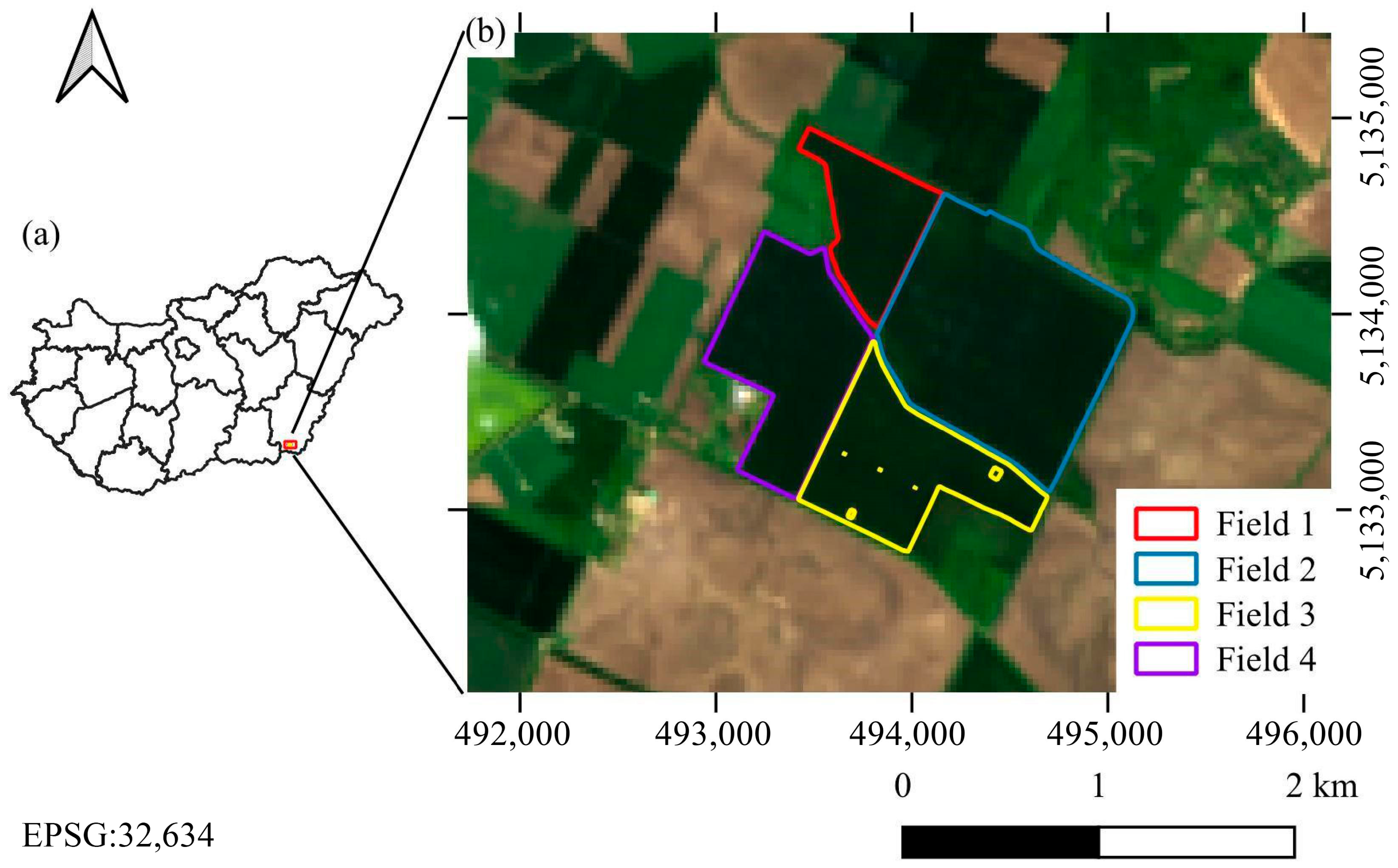
Figure 1. Study area: (a) Administrative boundary of Hungary and (b) true color composite from EnMAP hyperspectral sensor, acquired on 8 May 2023.
Remotesensing 17 03426 g001
Figure 2. Temporal dynamics of NDVI values (Sentinel-2) within the study area from October 2022 to May 2023.
Remotesensing 17 03426 g002
Figure 3. False color composite of the study area sown with winter wheat, based on EnMAP imagery acquired on (a) 23 February 2023 and (b) 8 May 2023. RGB channels correspond to R = 832 nm, G = 660 nm, and B = 560 nm.
Remotesensing 17 03426 g003
Figure 4. Observed yield data points aggregated to the EnMAP pixel grid for selected study fields. The yield measurements were averaged within each 30 m EnMAP pixel, providing spatially consistent estimates aligned with the hyperspectral imagery for subsequent analysis.
Remotesensing 17 03426 g004
Figure 5. Spectral signatures of high- and low-yield winter wheat EnMAP pixels in February.
Remotesensing 17 03426 g005
Figure 6. Spectral signatures of high- and low-yield winter wheat EnMAP pixels in May.
Remotesensing 17 03426 g006
Figure 7. Spatial variation in the narrow-band spectral indices on the study area: (a) gNDVI February; (b) gNDVI May; (c) GVMI February; (d) GVMI May; (e) SWIRVI February; and (f) SWIRVI May.
Remotesensing 17 03426 g007
Figure 8. Relative importance of vegetation indices for winter wheat yield estimation in February (single-date models).
Remotesensing 17 03426 g008
Figure 9. Relative importance of vegetation indices for winter wheat yield estimation in May (single-date models).
Remotesensing 17 03426 g009
Figure 10. Relative importance of vegetation indices for winter wheat yield estimation in multi-temporal data models (February and May).
Remotesensing 17 03426 g010
Figure 11. Scatter plots of predicted yield vs. observed yield from 30% validation. (a) February RF, (b) February GB, (c) February MLP, (d) May RF, (e) May GB, (f) May MLP, (g) multi-temporal RF, (h) multi-temporal GB, and (i) multi-temporal MLP. Performance metrics (MAE, R2), the 1:1 line (red), and the fitted line (black) are shown.
Remotesensing 17 03426 g011
Figure 12. Scatter plots of predicted yield vs. observed yield from 50% validation. (a) February RF, (b) February GB, (c) February MLP, (d) May RF, (e) May GB, (f) May MLP, (g) multi-temporal RF, (h) multi-temporal GB, and (i) multi-temporal MLP. Performance metrics (MAE, R2), the 1:1 line (red), and the fitted line (black) are shown.
Remotesensing 17 03426 g012aRemotesensing 17 03426 g012b
Table 1. Characteristics and spectral formulas of VIS/VNIR vegetation indices used in this study.
Index NameMain CategoryFormula
Anthocyanin Reflectance Index (ARI1)Carotenoids and anthocyanins(1/550 nm) − (1/700 nm)
Carotenoid Reflectance Index 2 (CRI2)Carotenoid content/plant stress(1/510 nm) − (1/700 nm)
Green Normalized Difference Vegetation Index (gNDVI)Vegetation chlorophyll content(550 nm − 800 nm)/(550 nm + 800 nm)
Hyperspectral NDVI (hNDVI)Chlorophyll content and structure(750 nm − 670 nm)/(750 nm + 670 nm) (with dynamically selected wavelengths)
Transformed Chlorophyll Absorption in Reflectance Index (TCARI)Chlorophyll content3 × ((700 nm − 670 nm) − 0.2 × (700 nm − 550 nm)) × (700 nm/670 nm)
Transformed Vegetation Index (TVI)Vegetation vigor√[(800 nm − 550 nm)/(800 nm + 550 nm) + 0.5]
Two-band Enhanced Vegetation Index (EVI2)Vegetation vigor2.5 × (800 nm − 650 nm)/(800 nm + 2.4 × 650 nm) + 1
Table 2. Characteristics and spectral formulas of SWIR-based vegetation indices used in this study.
Index NameMain CategoryFormula
Global Vegetation Moisture Index (GVMI)Vegetation moisture content((860 nm + 0.1) − (1240 nm + 0.02))/((860 nm + 0.1) + (1240 nm + 0.02))
Moisture Stress Index (MSI)Leaf water content1600 nm/820 nm
Normalized Difference Water Index (NDWI)Vegetation water content(860 nm − 1240 nm)/(860 nm + 1240 nm)
Shortwave Infrared Vegetation Index (SWIRVI)Dry matter/biomass37.27 × (2210 nm + 2090 nm) + 26.2
×(2208 nm − 2090 nm) − 0.57
Table 3. Model hyperparameters and configuration settings for RF, GB, and MLP algorithms.
ModelParameterValue/Type
Random Forest (RF)Number of trees500
Maximum depth15
Minimum leaf size5
Sampling strategyBagging
Random state42
Gradient Boosting (GB)Number of trees500
Maximum depth10
Minimum leaf size10
Learning rate0.3
Regularization (λ)1
Boosting strategySequential residual correction
Random state42
Multilayer Perceptron (MLP)Hidden layers(128, 64, 32) neurons
Activation functionReLU
OptimizerAdam
Learning rate0.001
Regularization (α, L2)0.001
Loss functionMean squared error
Maximum iterations500
Random state42
Disclaimer/Publisher’s Note: The statements, opinions and data contained in all publications are solely those of the individual author(s) and contributor(s) and not of MDPI and/or the editor(s). MDPI and/or the editor(s) disclaim responsibility for any injury to people or property resulting from any ideas, methods, instructions or products referred to in the content.