A Dual-Branch Framework Integrating the Segment Anything Model and Semantic-Aware Network for High-Resolution Cropland Extraction

Highlights

What are the main findings?

• A dual-branch framework (SAM-SANet) was proposed for high-resolution cropland extraction, integrating the Segment Anything Model with a Semantic-Aware Network to jointly capture global semantics and boundary details.
• The framework introduces the Boundary-aware Feature Fusion Module (BFFM) and the Prompt Generation and Selection Module (PGSM), which significantly improve boundary localization and segmentation accuracy across complex agricultural patterns.

What is the implication of the main finding?

• The proposed SAM-SANet extends the applicability of vision foundation models to high-resolution remote sensing segmentation, offering a general strategy for domain adaptation beyond natural images.
• By effectively combining semantic and boundary information, the framework enhances fine-scale cropland mapping and regional agricultural monitoring, contributing to precision agriculture and land resource management.

Abstract

Accurate spatial information of cropland is crucial for precision agricultural management and ensuring national food security. High-resolution remote sensing imagery combined with deep learning algorithms provides a promising approach for extracting detailed cropland information. However, due to the diverse morphological characteristics of croplands across different agricultural landscapes, existing deep learning methods encounter challenges in precise boundary localization. The advancement of large-scale vision models has led to the emergence of the Segment Anything Model (SAM), which has demonstrated remarkable performance on natural images and attracted considerable attention in the field of remote sensing image segmentation. However, when applied to high-resolution cropland extraction, SAM faces limitations in semantic expressiveness and cross-domain adaptability. To address these issues, this study proposes a dual-branch framework integrating SAM and a semantically aware network (SAM-SANet) for high-resolution cropland extraction. Specifically, a semantically aware branch based on a semantic segmentation network is applied to identify cropland areas, complemented by a boundary-constrained SAM branch that directs the model’s attention to boundary information and enhances cropland extraction performance. Additionally, a boundary-aware feature fusion module and a prompt generation and selection module are incorporated into the SAM branch for precise cropland boundary localization. The former aggregates multi-scale edge information to enhance boundary representation, while the latter generates prompts with high relevance to the boundary. To evaluate the effectiveness of the proposed approach, we construct three cropland datasets named GID-CD, JY-CD and QX-CD. Experimental results on these datasets demonstrated that SAM-SANet achieved mIoU scores of 87.58%, 91.17% and 71.39%, along with mF1 scores of 93.54%, 95.35% and 82.21%, respectively. Comparative experiments with mainstream semantic segmentation models further confirmed the superior performance of SAM-SANet in high-resolution cropland extraction.

1. Introduction

Efficient agricultural practices are a foundational pillar of national food security [1] and long-term ecological sustainability [2]. As the essential asset of agricultural production, cropland is vital not only for ensuring grain production [3] but also for supporting ecosystem services [4]. Therefore, obtaining timely and accurate information on the coverage and distribution of cropland is crucial for agricultural resource assessment and food security [5,6,7]. Remote sensing (RS) plays a key role in cropland mapping due to its capability of providing large-scale spatial coverage, high temporal resolution, and objective data acquisition [8,9]. Recent advances in high-resolution remote sensing (HRRS) imaging enabled the creation of important data sources for cropland mapping with a high level of thematic detail. However, despite the richness of information present in HRRS images, the high intraclass differences and low interclass diversity often encountered [10] make high-resolution cropland extraction challenging.

Traditional high-resolution cropland extraction methods rely heavily on image segmentation and hand-crafted features. They can be broadly categorized in object-based and region-based image analysis methods [11,12,13]. The object-based random forest method initially employs traditional image segmentation algorithms to isolate homogeneous objects, from which spectral, texture, and geometric features are then extracted. Finally, predefined classification rules based on these features are applied to identify cropland [11,12]. Region-based methods adopt an iterative aggregation strategy to group homogeneous pixels into objects, thereby producing highly continuous cropland boundaries [13]. Although the above methods are interpretable and adaptable through rule design, they are sensitive to image quality and scene complexity, which often leads to limited accuracy and generalization, particularly in high-resolution and heterogeneous cropland landscapes [14,15]. Moreover, their dependence on manual feature engineering and parameter tuning hinders scalability for large-scale, high-precision extraction tasks [16,17].

Due to its robust automatic feature extraction capabilities, deep learning has been widely applied in high-resolution cropland extraction [5,9,18]. Early deep learning models primarily adopted convolutional neural networks (CNNs), such as fully convolutional networks (FCNs), to achieve end-to-end pixel-level classification. The subsequent introduction of encoder–decoder architectures, incorporating dilated convolution modules and pyramid pooling modules, facilitated the development of classic semantic segmentation models like UNet and DeepLabV3+ [19,20]. These architectures significantly enhanced the models’ multi-scale feature representation and contextual reasoning capabilities. Through global context modeling, Transformer leveraging the self-attention mechanism have overcome the limitations of local receptive fields in traditional convolution operations [21]. This allows them to captures long-range pixel dependencies effectively and enhance discrimination of complex backgrounds and boundary details [22], further advancing the development of semantic segmentation models. Additionally, researchers have combined the local feature extraction advantages of CNN with the global relationship modeling capabilities of Transformer to develop remote sensing semantic segmentation models based on hybrid CNN-Transformer architectures. For example, Wang et al. [23] proposed UNetformer as a combination of a Transformer-based decoder with a lightweight CNN-based encoder for the efficient semantic segmentation of urban RS images. Wu et al. [24] proposed CMTFNet, which integrates CNNs with multiscale transformers to derive and unify local details and global-scale contextual information from HRRS imagery. Despite their strong performance in semantic segmentation tasks, these models face challenges in precise boundary delineation, particularly when capturing the irregular and intricate geometric features of cropland boundaries.

The Segment Anything Model (SAM), proposed by Meta AI in 2023 [25], represents a significant breakthrough in universal segmentation models. Trained on over millions of annotated images, SAM is exceptional in that it enables zero-shot segmentation of new visual objects without prior exposure. Although originally developed for natural images, SAM is being increasingly applied in the RS domain. However, since SAM’s segmentation results do not include class information, researchers typically use its raw mask predictions directly as priors for downstream semantic segmentation or boundary refinement, without altering SAM’s base architecture. For example, Sun et al. [26] employed SAM-generated masks combined with phenological feature recognition of crop outcomes to delineate crop boundaries. Ma et al. [27] developed a SAM-Assisted auxiliary semantic segmentation strategy, which employed an object consistency loss and boundary preservation loss based on SAM’s segmentation outputs, thus enhancing semantic segmentation performance. Nevertheless these methods rely heavily on SAM’s original outputs and lack adaptability for RS-specific tasks.

Recent studies have thus shifted toward adapting SAM for domain-specific tasks. For example, in the medical field, Lin et al. [28], introduced a CNN branch with cross-attention mechanisms in parallel with a Vision Transformer (ViT), along with feature and positional adapters, enabling the modified SAM to adapt to structured anatomical features like organs and lesions. However, HRRS imagery differs significantly from medical data in terms of object morphology and scene variability, as it typically exhibits large-scale variation, class heterogeneity, and irregular boundaries. To address these challenges, Chen et al. proposed RSPrompter [29], which learns the generation of prompt inputs for SAM, thereby enabling it to autonomously obtain semantic instance-level masks. Luo et al. [30] introduced an adapter to adapt a pretrained ViT backbone of SAM to RS images, and fine-tune the mask decoder by integrating bounding box information with multiscale features from the adapter to mitigate the significant domain shift from natural images. Sultan et al. [31] fine-tuned SAM using dense visual prompts from zero-shot learning and sparse visual prompts from a pre-trained CNN segmentation model, thus enabling the segmentation of mobility infrastructure including roads, sidewalks, and crosswalks. Wang et al. introduced SAMPolyBuild [32], a model that integrates an Auto Bbox Prompter for automatic object localization and extends the SAM decoder with multi-task learning capabilities to simultaneously predict segmentation masks, vertex maps, and boundary maps. Chen et al. presented ESAM [33], an edge-enhanced SAM variant specifically designed for photovoltaic (PV) power plant extraction. ESAM incorporates an edge detection module and a learning-based fusion strategy to effectively combine semantic and edge features, substantially improving segmentation accuracy. Ma et al. proposed a unified multimodal fine-tuning framework that leverages SAM’s generalizable image encoder and enhances it with Adapter and LoRA modules to process multimodal remote sensing data for semantic segmentation effectively [34]. Additionally, it is noteworthy that SAM’s fixed input size (1024 × 1024 pixels) leads to excessive computational resource consumption during training and low inference efficiency. To address this issue, Kato et al. proposed Generalized SAM [35], which supports variable input image sizes during fine-tuning through a positional encoding generator and introduces a spatial-multiscale AdaptFormer to enhance spatial feature modeling, reducing computational costs while maintaining segmentation performance. Specifically, GSAM leverages a learnable positional encoding generator composed of a convolution-based absolute positional embedding module and optional relative positional embeddings integrated into the attention blocks. These mechanisms enable GSAM to support variable input sizes during fine-tuning, but they introduce additional trainable parameters and rely on task-specific adaptation. Despite advancements in prompt design and architectural adaptation, research on SAM-based high-resolution cropland extraction remains limited. The aforementioned methods often focus on semantic or instance modeling, rarely addressing issues related to shape preservation and boundary continuity.

In summary, although current semantic segmentation models for high-resolution cropland extraction have achieved notable progress, they still suffer from insufficient accuracy in boundary localization. SAM is limited to generating segmentation results without class information, and directly applying the model to HRRS imagery semantic segmentation tasks may lead to poor adaptability. Therefore, in this study a dual-branch framework integrating SAM and a semantic-aware network (SAM-SANet) is proposed for high-resolution cropland extraction. The network utilizes a semantically aware branch based on semantic segmentation networks to recognize cropland regions, while a SAM-based branch incorporating boundary constraints is utilized to enhance the performance of cropland extraction. To tailor SAM for high-resolution cropland extraction, several modifications were made to its architecture. Specifically, a position embedding adapter (PEA) module is designed for the SAM-based branch, so that the network can accommodate image inputs of size, alleviating the computational overhead caused by SAM’s fixed input size. Additionally, a boundary-aware feature fusion module (BFFM) and a prompt generation and selection module (PGSM) are introduced into the SAM-based branch to enhance boundary accuracy and segmentation robustness. Furthermore, the images of a large-scale land-cover classification dataset, namely the Gaofen image dataset (GID) [36] are processed and reclassified into cropland and non-cropland, to construct the GID Cropland Dataset (GID-CD). Two study areas with distinct agricultural landscapes, namely Juye County and Qixia City in Shandong Province, were selected to create two cropland datasets, namely JY-CD and QX-CD. The effectiveness of the proposed SAM-SANet is evaluated comprehensively on these three datasets.

2. Datasets

This study employs three cropland datasets to assess the performance of the proposed approach in extracting high-resolution cropland regions. The first dataset is the GID Cropland Dataset (GID-CD), which is a reclassified version of the high-resolution land cover Gaofen Image Dataset (GID), released by Wuhan University. The other two datasets were constructed from study areas with distinct agricultural landscapes in Shandong Province, namely Juye County and Qixia City, and are referred to as the Juye Cropland Dataset (JY-CD) and the Qixia Cropland Dataset (QX-CD), respectively. These datasets provide a comprehensive basis for assessing the robustness of the proposed method across varying real-world scenarios. All datasets consisted of RS imagery and pixel-level cropland annotations, supporting training and evaluation for semantic segmentation tasks.

2.1. GID-CD

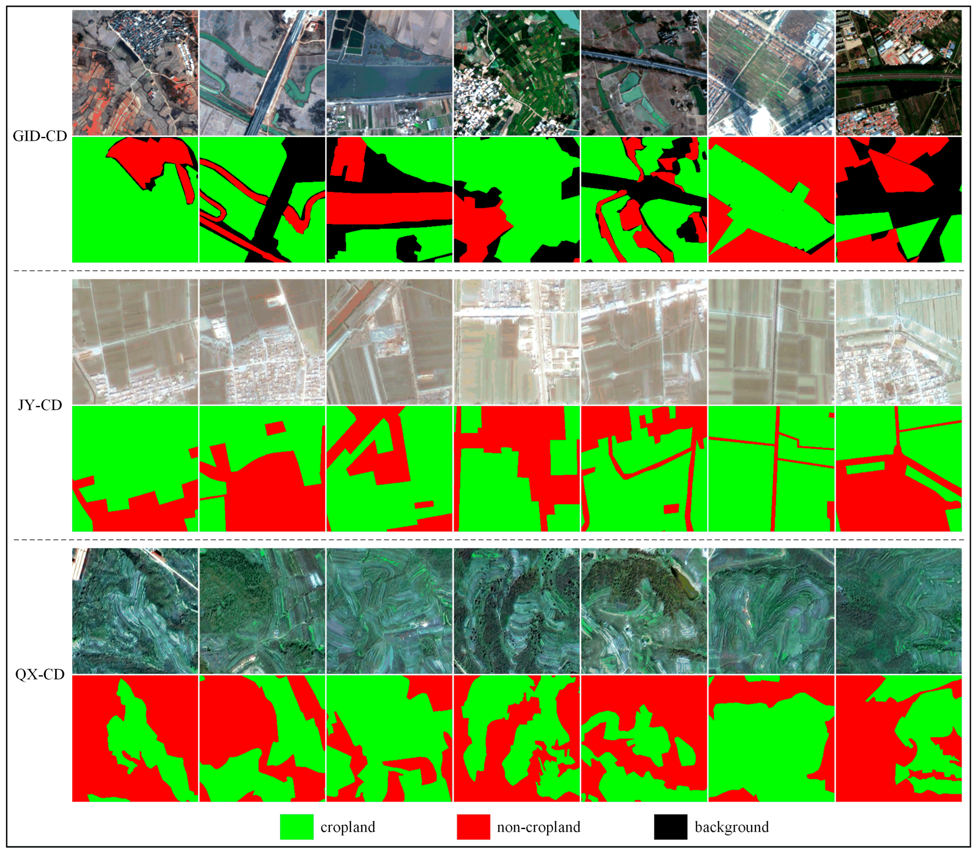
The original GID consists of 150 Gaofen-2 satellite images, each with a spatial resolution of 4 m and a size of 6800 × 7200 pixels, collectively covering more than 50,000 km² across over 60 cities in China. Each image covers approximately 506 km², and the geographic distribution of these scenes is detailed in the original GID publication [36]. The dataset included pixel-level annotations for five types of land cover, namely built-up, cropland, forest, grassland, and water, with areas not belonging to the above five classes and clutter regions are labeled as background. To facilitate cropland extraction, in this study the categories of the original dataset were redefined and integrated to construct the GID Cropland Dataset (GID-CD). Specifically, the “Cropland” and “background” categories from the original dataset are retained, while the other categories (i.e., “built-up”, “forest”, “grassland” and “water”) were merged into a single “non-cropland” category. After processing, a three-class dataset was formed, consisting of background (class 0), cropland (class 1), and non-cropland (class 2). To ensure the dataset contained valid cropland information, only satellite images with cropland area proportions greater than 15% were selected for the final GID-CD. Subsequently, the GID-CD dataset was split into non-overlapping patches of size 256 × 256, and samples with background proportions exceeding 50% were excluded. Ultimately, 46,994 samples were obtained in total and divided into training, validation, and test sets at a ratio of 8:1:1. These samples were drawn from the 150 Gaofen-2 scenes distributed over more than 60 cities in China, thus preserving the spatial diversity of the original GID and covering a wide range of geographic and cropland patterns. The GID-CD constructed in this study not only retains spatial details and texture characteristics of the initial high-resolution images, but also simplifies the classification process to enable models to focus on distinguishing cropland from non-cropland. It is therefore well-suited for the high-resolution cropland extraction tasks.

2.2. JY-CD and QX-CD

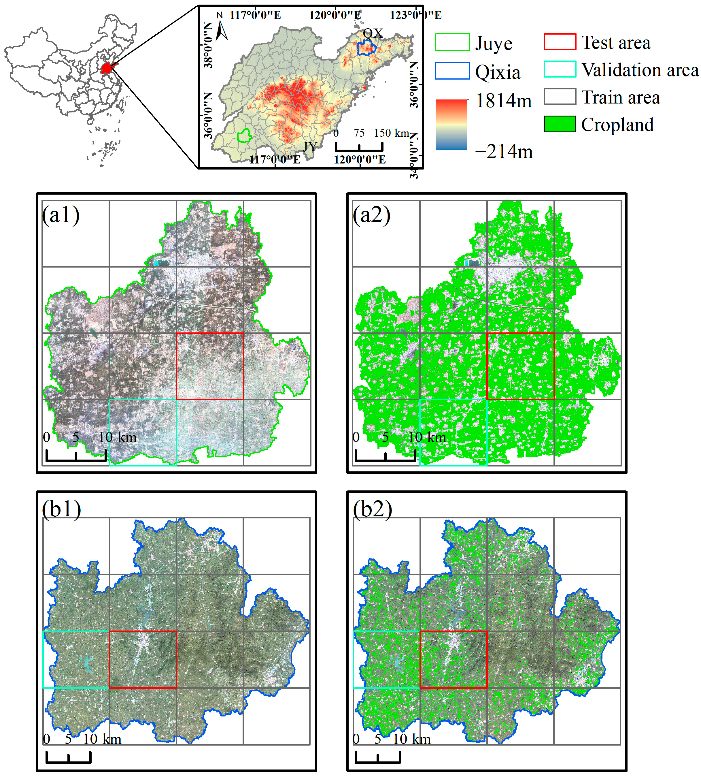
In addition to the GID-CD, which was constructed using a publicly available high-resolution land cover dataset, in this study two additional cropland datasets were constructed to validate the proposed method. Two study areas with distinct agricultural landscape characteristics were selected, namely Juye County (115°46′13″E–116°16′59″E, 35°6′13″N–35°29′38″N) and Qixia City (120°32′45″E–121°16′8″E, 37°5′5″N–37°32′57″N) in Shandong Province. The geographic locations of the study areas are shown in Figure 1.

Covering 1302 km², Juye County lies on the southwestern plain of Shandong Province, and is characterized by high agricultural productivity. It has a temperate continental monsoon climate with an average annual temperature of 13.8 °C and annual precipitation of 658 mm, concentrated from late June to September. Most of the land is dedicated to agriculture, while residential, grassland, forested, and water areas are also present to a lesser extent. The cropland parcels in the study area are relatively large and compact, making them suitable for intensive agricultural production. The crop calendar starts from early October to early or mid-June of the following year for winter wheat, and from April to October for spring and summer crops, which include maize, rice, soybean, millet, and cotton.

Qixia City is located in the northeastern Shandong Province, with an area of 1793 km². The climate is similar to that of Juye, with an average annual temperature of 11.7 °C and annual precipitation of 693 mm. The major land use/land cover types are forestry, agriculture, water, and residential. Hilly and mountainous terrain almost dominates the landscape, with irregularly distributed and fragmented agricultural fields. The typical crop rotation is winter wheat followed by spring and summer crops, which include maize, soybean, and peanut. Winter wheat is sown in early October and harvested in early or mid-June of the following year. Spring and summer crops are sown in late April and harvested from mid-September to early October.

This study used Gaofen-1 (GF-1) satellite images provided by the Land Satellite Remote Sensing Application Center (LASAC), Ministry of Natural Resources of the People’s Republic of China, as the remote sensing data source for cropland dataset construction. The spatial resolution of the satellite imagery is 2 m panchromatic (PAN)/8 m multispectral (MS). Then, the remotely sensed images were processed as composites with red, green, and blue bands at 2 m resolution through the fusion of the MS and corresponding PAN images using the Gram-Schmidt transformation, followed by applying the Albers Conical Equal Area projection. For Juye, GF-1 images acquired on 1 April 2016, were used, corresponding to the jointing stage of winter wheat, a period characterized by vigorous growth and significantly high vegetation coverage in the cropland areas (Figure 1(a1)). For Qixia, GF-1 images acquired on 22 August 2016, were used, corresponding to the silking stage of summer maize, which is a vigorous growth period where both forested and cropland areas demonstrate high vegetation coverage (Figure 1(b1)).

The cropland labels were constructed through visual inspection of the GF-1 composite data by professionals with RS experience. In Juye, non-cropland encompasses built-up, forest, water, road, meadow, greenhouse, and bare land, with built-up areas constituting the predominant non-cropland cover. Similarly, in Qixia, non-cropland included the same categories, with forests being the primary type of cover. A total of 19,147 (Juye) and 19,549 (Qixia) cropland parcels were delineated in the two study areas as ground truth data. The cropland parcel data were converted into raster format, setting “cropland” pixels to 1, “non-cropland” pixels to 2, and pixels without RS imagery coverage to 0—“background”. The GF-1 composite images and labeling results constituted the final cropland sample dataset. Consequently, two cropland datasets were created: the Juye Cropland Dataset (JY-CD) and the Qixia Cropland Dataset (QX-CD). Compared with the widely used GID-CD dataset, JY-CD and QX-CD were specifically constructed to represent two distinct and typical agricultural landscapes within Shandong Province. JY-CD corresponds to a flat plain region with concentrated and geometrically regular cropland parcels. In contrast, QX-CD is situated in a hilly and mountainous area, where cropland is fragmented, irregularly distributed, and surrounded by dense forest and complex terrain. These distinctions contribute to a broader representation of real-world scenarios and provide a more rigorous basis for evaluating the robustness of cropland extraction models under diverse geographic and agricultural conditions. A macro-grid-based splitting strategy was adopted based on the 16-sub-region grid illustrated in Figure 1. Entire grid cells were reserved as independent test regions (highlighted by red squares in Figure 1), thereby ensuring that no spatial overlap occurred between the training/validation regions and the test regions. Within the training and validation regions, a sliding-window approach with a 50% overlap and a patch size of 256 × 256 pixels was applied to generate a sufficient number of samples. Ultimately, 17,364 and 26,704 training sample blocks were obtained for JY-CD and QX-CD, and 1780 and 2659 validation sample blocks, respectively. Figure 2 shows some typical samples of the three high-resolution cropland datasets GID-CD, JY-CD, and QX-CD.

3. Methodology

3.1. Proposed SAM-SANet Architecture

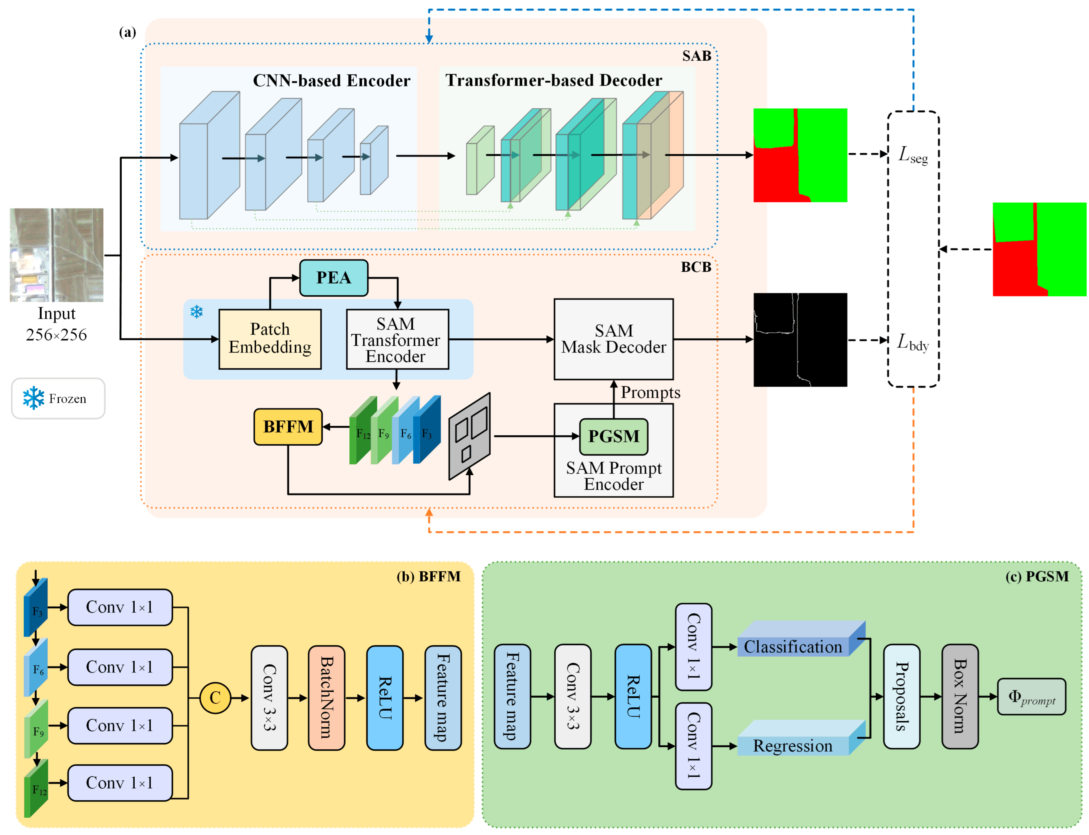
The overall architecture of SAM-SANet, shown in Figure 3, is mainly composed of two components: the semantically aware branch (SAB) and the SAM-based boundary-constrained branch (BCB). The SAB utilizes the UNetFormer architecture for semantic segmentation to precisely recognize cropland regions, while the BCB refines the SAM framework to enhance its suitability for locating cropland boundaries. Within the BCB, a position-embedding adapter (PEA) is integrated into the image encoder to address the input size mismatch caused by the fixed positional encoding in SAM. To fully leverage the general visual representation capability of the SAM pretrained encoder, the encoder parameters are frozen during training and shallow and intermediate multi-scale features from the Transformer are fused through the boundary-aware feature fusion module (BFFM), thereby enhancing boundary representations and improving the model’s suitability for RS-based cropland boundary extraction. In the prompt encoder of SAM, the prompt generation and selection module (PGSM) generates high-quality box prompts, which help the decoder focus more effectively on boundary structures and improves the precision of cropland boundary delineation. Finally, class tokens are also incorporated into the SAM decoder to enable semantic information modeling, thereby achieving more precise boundary localization at the cropland region level. Notably, the UNetFormer architecture used in the SAB can be replaced by other mainstream semantic segmentation networks. Since the optimization of the SAB is not the primary focus of this study, the analysis focuses on the adaptation of the SAM structure, with particular emphasis on the design and function of the BCB sub-modules for boundary perception.

In summary, the proposed SAM-SANet incorporates the SAM-based BCB on top of the semantic segmentation network to enhance cropland extraction performance. A dual-loss mechanism is employed during training to jointly optimize the outputs of both branches, while the final cropland extraction results are produced by the SAB based on the semantic segmentation network during the inference phase.

3.2. Boundary-Constrained Branch (BCB)

3.2.1. Position Embedding Adapter

The image encoder in SAM is based on the Vision Transformer (ViT) architecture, which employs a set of learnable absolute positional embeddings that are tightly coupled with a fixed input size. The positional embeddings are typically trained on a fixed size (e.g., 1024 × 1024), thereby restricting the original SAM to fixed-size image inputs. This limitation becomes particularly pronounced in the domain of RS image segmentation, especially in fine-grained tasks such as cropland boundary extraction, where precise spatial representation is essential. The fixed size can impose an excessive computational burden, and this constraint significantly hinders the model’s multi-scale adaptability and practicality during deployment.

To address this issue, in this study, the addition of a position embedding adapter (PEA) is proposed during the positional encoding injection stage. The goal of PEA is to adapt the fixed-size absolute positional embeddings to input sizes without requiring the modification of the pre-trained embedding structure or additional training. The core idea is to treat the original positional embedding matrix as a two-dimensional feature map and apply bilinear interpolation to rescale it spatially. This operation preserves the continuity and semantic consistency of the positional embeddings, while increasing practicality due to the flexible input sizes. Notably, the PEA module does not involve any learnable parameters and performs a single interpolation operation prior to encoding. By interpreting the absolute positional embedding as a two-dimensional spatial feature map and applying bilinear interpolation, the spatial relationships and alignment patterns embedded in the original matrix are preserved across varying input sizes, ensuring semantic continuity in downstream feature encoding.

Let the original position embedding tensor be denoted as $E_{\mathrm{ori}}\in {ℝ}^{L_{\mathrm{ori}}\times C}$. The PEA module first reshapes it into a four-dimensional tensor of shape [1, C, H_ori, W_ori], applies bilinear interpolation to resize it to (H_new, W_new), and then flattens the result to [L_new, C]:

$$E_{\mathrm{new}}=\mathrm{Ft} (\mathrm{Intp}(\mathrm{R}(E_{\mathrm{ori}}),H_{\mathrm{new}},W_{\mathrm{new}}))$$

(1)

where L_ori = H_ori × W_ori and L_new = H_new × W_new represent the sequence lengths of the original and target input sizes, respectively. C is the embedding dimension, R(·) denotes the reshaping operation, Intp(·) represents bilinear interpolation, and Ft(·) denotes the flattening operation.

The proposed PEA module allows high-resolution remote sensing images to be directly input into the SAM image encoder at sizes adapted to the target dataset (e.g., 256 × 256 in our case). This effectively allows transferring the pre-trained ViT-based encoder to input scenarios specific to cropland boundary extraction, enhancing the model’s flexibility and adaptability in remote sensing applications.

3.2.2. Boundary-Aware Feature Fusion Module

The outputs of different Transformer layers in the ViT-based encoder of SAM exhibit varying levels of semantic abstraction. Shallow Transformer layers tend to capture local structures and fine-grained details, particularly the textures and contours of cropland boundaries. Although these layers are sensitive to edge cues, they lack semantic and contextual constraints, which makes them prone to noisy or fragmented boundary responses, especially in complex cropland scenes with shadows, texture overlaps, or background clutter. In contrast, deeper Transformer layers focus more on global semantic modeling, enabling the perception of the overall structure and contextual semantics of cropland regions. These intermediate and deep layers encode larger receptive fields and stronger semantic priors, which help suppress false boundary activations and enhance region-level consistency. Therefore, fusing multi-level features allows the model to construct boundary representations that are both fine-grained and semantically coherent, effectively enhancing its ability to extract complex cropland boundaries [37,38]. To address this, the boundary-aware feature fusion module (BFFM) (Figure 3b) is proposed, which explicitly integrates shallow, intermediate and deep multi-scale Transformer features to construct a fused representation with strong boundary sensitivity, thereby improving the model’s capability to detect detailed cropland edges.

Specifically, let the output feature maps from different Transformer layers be denoted as

$${\left\{F_i\right\}}_{i=3,6,9,12}^n,F_i\in {ℝ}^{C\times H\times W}$$

(2)

where i = 3, 6, 9, 12 correspond to the shallow, intermediate, and deep layers of the ViT-b encoder, which are selected to capture complementary information: fine-grained textures (3rd), regional semantics (6th and 9th), and global contextual information (12th). C is the channel dimension and H, W denote the spatial resolution. Each feature map F_i comes from a specific Transformer layer, capturing features at distinct levels of semantic granularity.

First, 1 × 1 convolution layers are applied to individually project the extracted shallow and middle-layer feature maps into the same channel dimension, achieving the initial alignment and unification of the features.

$$F_i^{\prime }={\mathrm{Conv}}_{1\times 1}(F_i)$$

(3)

Subsequently, the dimension-reduced feature maps from the different layers are concatenated along the channel dimension to fuse boundary and semantic information across levels. This results in the multi-level fused feature map F_c, which incorporates rich cropland boundary textures from shallow to middle layers, and can therefore significantly enhancing its capability to represent complex cropland boundaries. To further integrate the fused features and smooth the spatial representations, a 3 × 3 convolution is applied, followed by a Batch Normalization layer to stabilize training and accelerate convergence. A ReLU activation is then employed to introduce non-linearity. The final fused feature map is denoted as F_b, where

$$F_{\mathrm{c}}=\mathrm{Concat}(\{F_i^{\prime }\})$$

(4)

$$F_{\mathrm{b}}=\mathrm{ReLU}(\mathrm{BN}({\mathrm{Conv}}_{3\times 3}(F_{\mathrm{c}})))$$

(5)

The boundary-aware feature fusion module integrates cropland information at different levels of abstraction, with a particular emphasis on accurate boundary representation. This multi-level fusion strategy lays an important foundation for the subsequent PGSM, which is used to generate high-quality object prompt embeddings.

3.2.3. Prompt Generation and Selection Module

In RS imagery, cropland boundaries typically exhibit regular or semi-regular spatial structures. When a foundation model like SAM is employed, the accuracy of the segmented images’ boundaries depends largely on the quality of prompts fed into the prompt encoder. Low-quality prompts often fail to cover complex boundary regions, resulting in segmentation errors and significantly reducing the effectiveness of boundary guidance. To address this issue, in this paper, the prompt generation and selection module (PGSM) is proposed, as illustrated in Figure 3c. This module is designed to select high-quality boundary-aware prompts from candidate regions, thereby enhancing SAM’s capability to perceive fine-grained boundary details and reinforcing its boundary attention within the mask decoder. Structurally, the PGSM draws inspiration from classical region proposal networks (RPN) used in object detection. The Region Proposal Network (RPN) is a fully convolutional module widely used in object detection frameworks that simultaneously predict objectness scores and bounding box coordinates at each sliding-window location on the feature map. The extracted features are fed into two sibling layers: a classification layer that predicts the objectness score and a regression layer that outputs the bounding box coordinates [39]. Typically, the proposals generated by the RPN are processed by RoI pooling (or RoIAlign) to produce fixed-size feature representations, which are then forwarded to subsequent layers for classification and bounding-box regression [40]. In contrast, the proposed PGSM focuses solely on producing sparse, high-confidence proposals to guide the segmentation model, without coupling with downstream region classification or detection heads.

Specifically, in PGSM, anchors are initialized on a regular grid over the feature map Fb, with one center-aligned square anchor per spatial location. The anchor size is set equal to the feature-map stride, yielding a one-to-one correspondence between each anchor and the receptive field of a feature-map location. This design ensures dense and uniform spatial coverage without overlap gaps and allows the model to fully exploit the local boundary information encoded in Fb. These anchors are subsequently refined via classification and regression branches, whose parameters are indirectly optimized during the overall model backpropagation process, thereby receiving implicit supervision without relying on explicit ground-truth bounding boxes.

Specifically, a 3 × 3 convolution is applied on the boundary-aware feature map F_b to extract local spatial features, followed by a ReLU activation function to obtain the intermediate feature representation F_r. Subsequently, two separate 1 × 1 convolutional heads are employed to predict the foreground probability distribution of anchors and the corresponding bounding box offsets. The outputs of these operations are those obtained by the foreground classification and the bounding box regression branches, respectively, and formally defined as follows:

$$F_{\mathrm{r}}=\mathrm{ReLU}{\mathrm{Conv}}_{3\times 3}\left(F_{\mathrm{b}}\right)$$

(6)

$$P_{\mathrm{obj}}=\mathrm{Softmax}({\mathrm{Conv}}_{1\times 1}^{\mathrm{cls}}(F_{\mathrm{r}}))$$

(7)

$${\Delta }_{bbox}={\mathrm{Conv}}_{1\times 1}^{\mathrm{reg}}(F_{\mathrm{r}})$$

(8)

where P_obj denotes the probability distribution indicating the likelihood of each anchor belonging to the foreground, while ${\Delta }_{bbox}$ represents the bounding box regression offsets relative to the initial position of the anchor.

To reduce redundancy, only the highest foreground scores are retained as the final set of high-confidence proposal boxes. Their coordinates are then normalized to the range [0, 1], and the normalized boxes are passed into the prompt head ${\mathrm{\Phi }}_{prompt}$ to generate the corresponding prompt embedding vectors. Instead of applying a fixed probability threshold, we rank all anchors by their predicted foreground probabilities and retain the top-K per image (set to 32 in our experiments). This ranking-based selection ensures that each image contributes a consistent number of high-confidence prompts, preventing sample imbalance in sparse cropland scenes and suppressing noisy low-confidence anchors.

Compared with conventional RPNs and other prompt generation strategies, PGSM is more lightweight and is specifically tailored for prompt generation rather than object detection. Furthermore, unlike random or grid-based prompt sampling methods commonly used in SAM, PGSM adaptively selects proposals guided by boundary-aware features, and as a result, the high-response foreground regions generated by this module effectively capture the contextual structure of cropland boundaries, which are subsequently transformed into sparse prompt embeddings and fed into the SAM mask decoder.

3.3. Semantically Aware Branch (SAB)

In the SAB, a UNetFormer [23] architecture is incorporated for large-scale semantic representation and extraction of cropland regions. This architecture is chosen for its ability to effectively combine local and global contextual information. The architecture adopts an encoder–decoder structure. The encoder consists of multiple convolutional layers that perform progressive downsampling to capture both shallow texture and deep semantic features effectively, and is thus able to process the morphological complexity and scale variability of cropland regions. The decoder is formed through the stacking of transformer blocks, integrating local-global self-attention mechanisms to model long-range pixel dependencies. Finally, skip connections are established between corresponding encoder and decoder layers to fuse their features, preserving fine-grained local details and enhancing the segmentation accuracy of cropland regions.

3.4. Loss Function

To jointly optimize semantic segmentation accuracy and boundary localization capability, a composite loss function composed of both segmentation and boundary loss was adopted. The segmentation loss focuses on pixel-wise classification between cropland and non-cropland regions, while the boundary loss improves the model’s ability to perceive and delineate edge structures. Through this dual-branch collaborative optimization, regional semantics and high-precision boundaries are unified effectively.

3.4.1. Segmentation Loss

The SAB is optimized using cross-entropy loss, which guides the model to learn accurate pixel-level classification. Let $\widehat{y}$ denote the predicted output and y the corresponding ground truth label. The segmentation loss is defined as

$$L_{\mathrm{seg}}=-\sum _{i=1}^{H\times W}\sum _{c=1}^L{y}_{i,c}\log {\widehat{y}}_{i,c}$$

(9)

where $y_{i,c}$ represents the ground truth label of pixel i for class c, and ${\widehat{y}}_{i,c}$ denotes the predicted probability for the same class.

3.4.2. Boundary Loss

To improve the accuracy of boundary localization, a boundary-aware loss function is introduced for the BCB based on the boundary F1-score (BF1). To ensure the differentiability of this loss during gradient-based optimization, the predicted soft boundary map P_b is obtained through the application of a boundary extraction operator to the soft segmentation probability output, while the ground truth boundary map G_b is derived via the extraction of the boundary from the binarized ground truth label. The soft boundary precision $\mathcal{P}$, recall $\mathcal{R}$, boundary F1-score, and boundary loss are defined as follows:

$$\mathcal{P}={\displaystyle \frac{\sum (P_b\cdot G_b)}{\sum P_b+\epsilon }},\mathcal{R}={\displaystyle \frac{\sum (P_b\cdot G_b)}{\sum G_b+\epsilon }}$$

(10)

$$\mathrm{BF}1={\displaystyle \frac{2\cdot \mathcal{P}\cdot \mathcal{R}}{\mathcal{P}+\mathcal{R}+\epsilon }}$$

(11)

$$L_{\mathrm{bdy}}=1-\mathrm{BF}1$$

(12)

where $\mathcal{P}$ denotes the ratio of predicted boundary pixels that overlap with the ground truth boundary pixels correctly, and $\mathcal{R}$ represents the ratio of ground truth boundary pixels that are successfully captured by the predicted boundary. A greater boundary F1-score implies improved consistency between the predicted and reference boundaries, thereby facilitating more accurate contour delineation. The term $\epsilon$ is a small constant added to prevent division by zero.

3.4.3. Total Loss

Finally, the total loss optimized during model training is formulated as a weighted combination of the semantic segmentation loss and the boundary loss:

$$L_{\mathrm{total}}=L_{\mathrm{seg}}+\lambda \cdot L_{\mathrm{bdy}}$$

(13)

where λ is a weighting coefficient for the boundary loss, treated as a tunable hyperparameter in this study, which controls the relative contribution of the boundary loss to the overall segmentation objective.

This dual-branch supervision strategy facilitates the simultaneous optimization of both semantic expression and boundary alignment, thereby improving segmentation accuracy and edge integrity in cropland extraction tasks.

3.5. Comparison Methods

To assess the performance of the proposed approach in cropland extraction comprehensively, two popular general semantic segmentation models (UNet [19] and DeepLabV3+ [20]) and three representative RS semantic segmentation models (UNetFormer, FTUNetFormer [23], CMTFNet [24] and DFormerv2 [41]) were selected as baseline comparisons. These methods span a diverse range from conventional CNN architectures to hybrid models incorporating Transformer modules. UNet, a classical symmetric convolutional network, leverages skip connections to preserve spatial details effectively, making it well-suited for segmentation tasks with regular structural patterns. On the other hand, DeepLabV3+ adopts a dilated spatial pyramid pooling structure to gather multi-level contextual cues, thus improving segmentation performance in scale-variant regions. UNetFormer and FTUNetFormer integrate the complementary strengths of CNNs and Transformer. The former employs convolutional encoders for local texture extraction with Transformer-based decoders, whereas the latter further enhances this framework with fine-tuning strategies to improve domain adaptability in remote sensing. CMTFNet incorporates multi-scale Transformer modules to capture long-range dependencies and achieve unified modeling of global and local features. DFormerv2 leverages depth as a geometric prior to guide a geometry self-attention mechanism, thereby enhancing context modeling and improving segmentation performance. In addition, SAM [25] and its fine-tuned variants, GSAM [35] and SAMUS [28], are included, which adapt the Segment Anything framework to specific semantic segmentation tasks. GSAM improves training efficiency by enabling variable input image sizes, while SAMUS integrates a parallel CNN branch with cross-attention and adapter modules to improve adaptation to structured and fine-grained objects. All baseline models have demonstrated strong general performance in segmentation tasks and serve as a solid reference for assessing the strengths of the proposed method.

3.6. Model Implementation

All experiments were conducted using the PyTorch 2.2.2 deep learning framework (CUDA 12.1). To maintain hardware consistency and training stability, all models were trained and evaluated on a system equipped with dual NVIDIA RTX 4070 Ti GPUs. The optimization process utilized stochastic gradient descent with a starting learning rate of 0.01, momentum of 0.9, and a weight decay parameter of 0.0005. A multi-step learning rate scheduler progressively decayed the learning rate by a factor of γ = 0.1 at the 25th, 35th, and 45th epochs. Training was conducted for a total of 50 epochs, with a fixed batch size of 4. The boundary loss weight λ was tuned separately for each dataset based on boundary sensitivity analysis to better accommodate terrain-specific boundary refinement. After each epoch, the mean Intersection over Union (mIoU) was calculated on the validation dataset. The model that obtained the best validation mIoU was chosen for subsequent evaluation to ensure optimal performance.

3.7. Evaluation Metrics

To comprehensively evaluate the model’s performance in semantic segmentation, the assessment involved four widely adopted metrics, namely IoU, F1-score, Kappa, and overall accuracy (OA). Their specific definitions are as follows:

$$\mathrm{IoU}={\displaystyle \frac{TP}{TP+FP+FN}}$$

(14)

$$\mathrm{F}1={\displaystyle \frac{2TP}{2TP+FP+FN}}$$

(15)

$${\mathrm{p}}_{\mathrm{e}}={\displaystyle \frac{(TP+FP)\times (TP+FN)\times (TN+FP)\times (TN+FN)}{{(TP+FP+TN+FN)}^2}}$$

(16)

$$\mathrm{Kappa}={\displaystyle \frac{\mathrm{OA}-{\mathrm{p}}_{\mathrm{e}}}{1-{\mathrm{p}}_{\mathrm{e}}}}$$

(17)

$$\mathrm{OA}={\displaystyle \frac{TP+TN}{TP+TN+FP+FN}}$$

(18)

where true positives (TP) and true negatives (TN) denote the number of pixels correctly classified as positive and negative categories, respectively, while false positives (FP) and false negatives (FN) indicate the number of non-target pixels that are erroneously assigned to the positive or negative classes. The p_e denotes the expected accuracy, computed as the sum of the products of actual and predicted pixel counts across all categories, divided by the square of the total number of pixels.

To characterize the geometric complexity of cropland boundaries, this study introduced the indicator “boundary tortuosity” [42,43,44] which quantifies the degree of irregularity or twisting in a region’s boundary. It is defined as

$$\mathrm{Tortuosity}={\displaystyle \frac{\mathrm{P}}{2\mathrm{\pi }\sqrt{\mathrm{A}/\mathrm{\pi }}}}$$

(19)

where P is the actual perimeter of the region, and A is the region area. The denominator is the circumference of a circle with the same area, representing the most compact possible shape. A tortuosity value of 1 indicates a perfectly circular region, while values greater than 1 reflect increasing boundary irregularity.

To further assess the model’s complexity and computational efficiency, we introduce two supplementary indicators: the number of model parameters (Params) and giga floating-point operations (GFLOPs) [45]. Params quantifies the total number of learnable weights, while GFLOPs measures the number of arithmetic operations required to process a single input, reflecting the model’s inference cost. Lower GFLOPs generally indicate faster inference and reduced resource consumption. Both metrics are calculated using the THOP library, which profiles PyTorch models by analyzing their structure during a single forward pass.

4. Results

4.1. Cropland Extraction Results

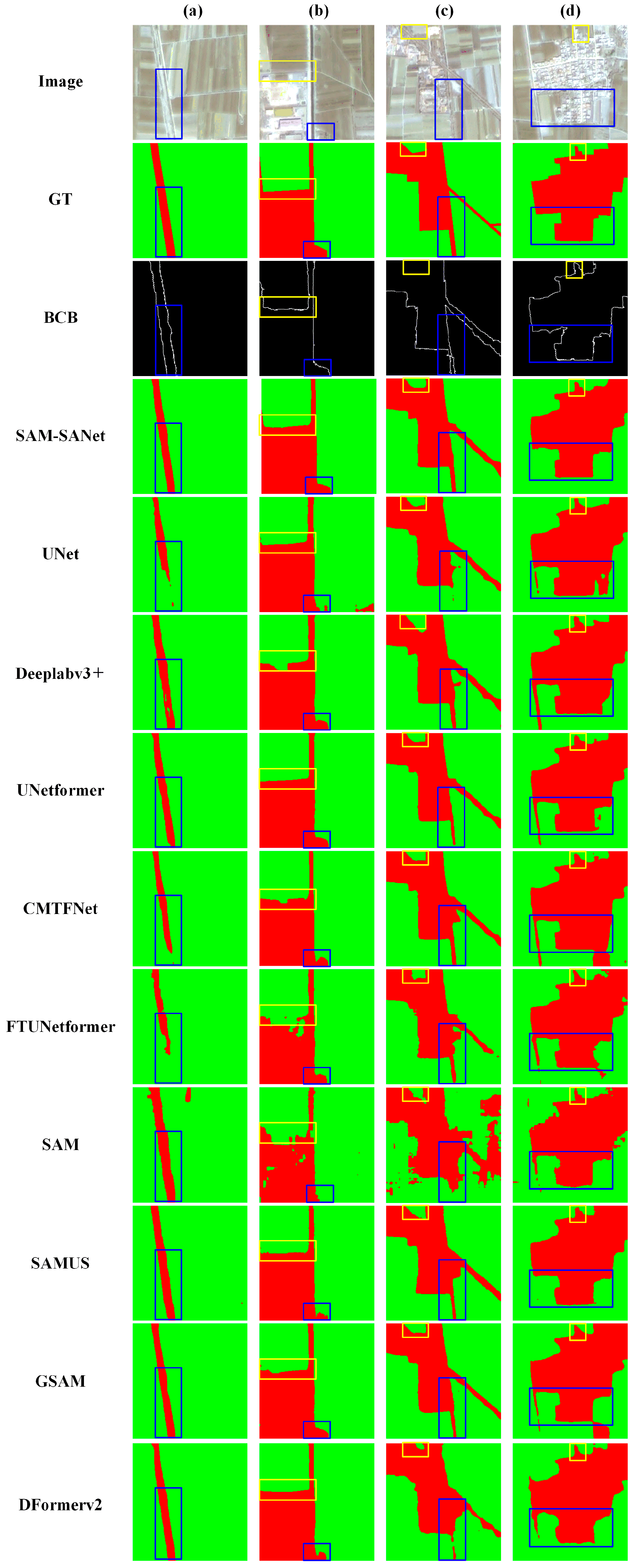
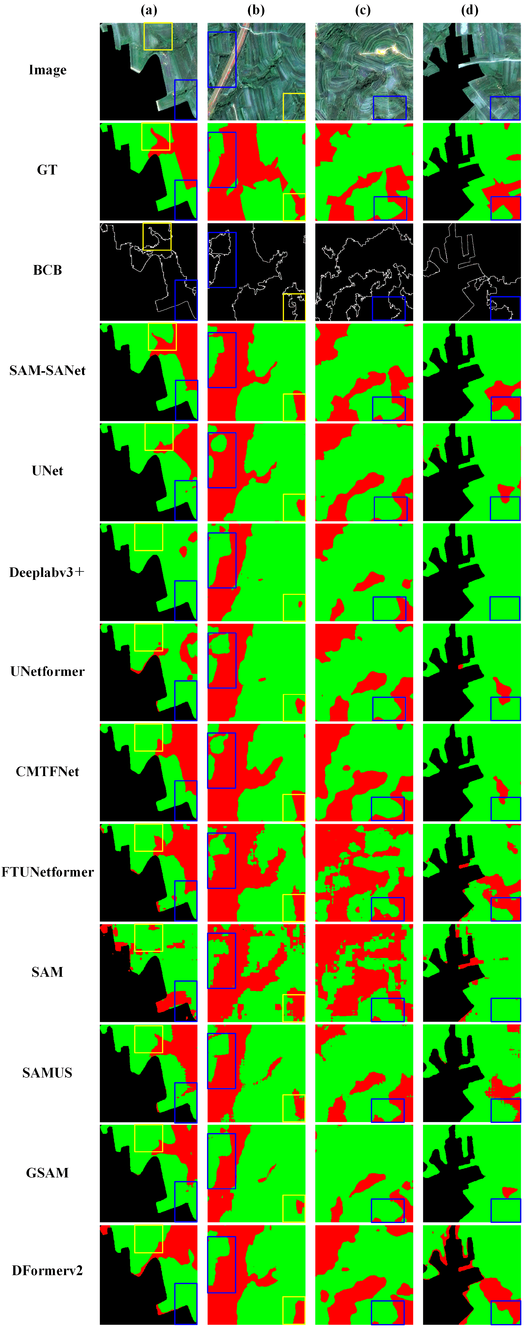
To evaluate the segmentation performance of the proposed method across diverse terrain types and image complexities, qualitative visual comparisons between the proposed model and the other comparison were conducted using the three representative datasets discussed in Section 2, namely GID-CD, JY-CD, and QX-CD. For each dataset, representative samples were selected to assess model performance in terms of boundary preservation, object integrity, and detail recovery. Figure 4, Figure 5 and Figure 6 show the segmentation results of various comparison models, along with the intermediate boundary maps generated by the boundary-constrained BCB of SAM-SANet and its final segmentation outputs.

Figure 4 shows the prediction results for representative samples of GID-CD (The blue and yellow boxes mark representative regions that were manually selected to facilitate the visual comparison of segmentation performance across different models). In Figure 4a, SAM-SANet demonstrated strong cropland boundary extraction in regions where water bodies, roads, and cropland intersect, while avoiding misclassification effectively. In contrast, other methods produced blurred or ambiguous segmentation along riverbanks. Notably, although SAM and its variants, SAMUS and GSAM, partially preserved boundary shapes in complex transition zones, they still exhibited fragmented or noisy edges, especially around river boundaries. In Figure 4b, the elongated cropland boundaries exhibited varying degrees of overflow or blurring in UNet and DeepLabV3+. SAM and its variants still struggled to maintain spatial continuity in long narrow plots compared to SAM-SANet, whereas SAM-SANet restored the cropland boundary shapes precisely and delineated the cropland regions accurately. In Figure 4c, extensive cropland regions are interlaced with grassland and forest regions, the BCB captured cropland boundaries effectively, thereby assisting the semantic segmentation network in generating clearer cropland segmentation results. In Figure 4d, large cropland regions are distributed within a heterogeneous background. SAM-SANet effectively preserves fine-grained boundary contours and accurately delineates adjacent cropland and non-cropland regions, thereby avoiding over-merging. In contrast, UNet and CMTFNet tend to merge spatially adjacent but semantically different regions, DeepLabV3+ and UNetFormer additionally exhibit misclassification of non-cropland and background regions. While SAMUS and GSAM incorporate structural improvements over the original SAM, they still fail to maintain boundary integrity in large and heterogeneous cropland clusters, resulting in partial over-segmentation or class confusion. Compared with these methods, SAM-SANet yields segmentation results that better match the ground truth in preserving intra-class structural separation. Overall, with the constraint of the BCB, SAM-SANet exhibited enhanced boundary preservation and spatial consistency in HRRS imagery with complex and heterogeneous backgrounds. These results highlight the model’s strong adaptability in real-world cropland extraction tasks.

Figure 5 shows the prediction results for representative samples of JY-CD. In Figure 5a, the blue box highlights a narrow and relatively regular non-cropland strip. SAM-SANet accurately reconstructed its boundary morphology, maintaining clear and continuous boundaries. In contrast, UNet and DeepLabV3+ exhibited boundary breaks and blurred expansion. While UNetFormer and CMTFNet yielded more coherent shape predictions, their segmentation boundaries were still spatially misaligned with actual object edges and tended to slightly over-extend in narrow non-cropland regions. In Figure 5b, many methods of the comparison showed over-segmentation or boundary swelling, whereas SAM-SANet successfully distinguishes narrow gaps between cropland and adjacent roads or buildings, thereby avoiding over-expansion of predicted cropland regions. In Figure 5b,c, compared with these methods, the original SAM produced fragmented and noisy responses, whereas SAMUS and GSAM partially alleviated these issues and achieved fine-grained edge alignment comparable to SAM-SANet. In Figure 5c,d, SAM-SANet exhibited precise separation of adjacent cropland and non-cropland regions with sharp and continuous cropland boundaries. Other methods tended to blend boundary regions or produce broken and distorted cropland region shapes. In Figure 5d, the SAM-derived variants achieved partial improvements in boundary clarity but remained inferior to SAM-SANet in maintaining consistent cropland shapes. In summary, these results indicate that the BCB is capable of accurately delineating cropland boundaries in flat plain areas with relatively simple cropland morphology. It effectively captured subtle structural changes between cropland and non-cropland regions, thereby enabling SAM-SANet to produce more accurate cropland segmentation results.

Figure 6 shows the prediction results for a representative sample of QX-CD. In Figure 6a, SAM-SANet accurately predicted continuous and clear boundaries on these complex and curved mountainous cropland regions, whereas most comparison methods produced fuzzy or misclassified boundaries in the same area. In Figure 6b, conventional semantic segmentation networks exhibited varying degrees of over-segmentation and spatial ambiguity. Among them, CMTFNet and SAM-SANet achieved slightly more accurate boundary localization in the highlighted regions, particularly in delineating narrow forest margins. A comparison with UNetFormer further demonstrates that the integration of BCBs and SABs enables SAM-SANet to achieve clearer separation between cropland and surrounding forest areas across most regions. In Figure 6a–c, the original SAM struggled to adapt to the fragmented terrain, yielding broken or noisy boundary predictions. SAMUS and GSAM alleviated some of these errors and generated more regular shapes, but their boundary delineation remained less precise than that of SAM-SANet. In Figure 6d, SAM-derived variants showed partial improvements but still misclassified narrow forest margins as cropland, whereas SAM-SANet maintained clearer distinctions. As further shown in Figure 6c,d, the performance of the BCB in delineating cropland boundaries was significantly affected by the complex forest interference in this dataset, resulting in a notably lower accuracy compared to more regular and flat cropland terrain, such as in the GID-CD and JY-CD datasets. Nevertheless, SAM-SANet still demonstrated better boundary localization than other models, indicating that the BCB provided a certain degree of boundary constraint ability. Overall, under conditions of severe natural boundary variation and diverse terrains, the BCB provided limited yet beneficial guidance, enabling SAM-SANet to achieve relatively improved cropland segmentation performance.

4.2. Accuracy Assessment

To evaluate the adaptability of the proposed method comprehensively across different types of RS scenarios, a comparative accuracy analysis was conducted on the three datasets—GID-CD, JY-CD, and QX-CD—to assess the model’s cropland extraction performance under conditions of complex backgrounds, regular parcels, and fragmented terrain.

The GID-CD dataset was employed to assess the cropland extraction capability of SAM-SANet under large-scale and complex interference conditions. As shown in

Table 1. Accuracy comparison of different models on GID-CD. All evaluation metrics are presented in percentage format (%).

Method		Cropland-IOU/F1	Non-Cropland-IOU/F1	MIOU	MF1	Kappa	OA
CNN/Transformer-based	Unet	88.70/94.01	84.79/91.77	86.74	92.89	81.39	89.54
	Deeplabv3+	88.50/93.89	84.48/91.58	86.49	92.73	80.89	89.28
	UNetformer	88.64/93.98	84.95/91.86	86.79	92.92	81.49	89.56
	CMTFNet	88.51/93.90	84.80/91.78	86.65	92.84	81.31	89.44
	FTUNetformer	87.54/93.35	83.67/91.11	85.61	92.23	79.47	88.54
	DFormerv2	88.81/93.93	85.19/91.88	87.00	92.91	82.39	89.93
SAM-based	SAM	83.40/90.94	75.93/86.32	79.67	88.63	72.71	84.79
	SAMUS	89.49/94.45	85.13/91.97	87.31	93.21	82.47	90.15
	GSAM	89.57/94.50	85.35/92.09	87.46	93.29	82.54	90.22
	SAM-SANet	89.31/94.53	85.85/92.55	87.58	93.54	82.37	90.25

(optimal scores highlighted in bold), SAM-SANet achieved an IoU of 89.31% and an F1-score of 94.53% for the cropland category, maintaining excellent accuracy in cropland extraction even on large HRRS images. For the non-cropland category, SAM-SANet obtained an IoU of 85.85% and an F1-score of 92.55%, further demonstrating its strong capability in discriminating heterogeneous targets such as buildings, grassland and water bodies from cropland. Regarding overall metrics, SAM-SANet achieved a mean IoU (mIoU) of 87.58%, a mean F1 score (mF1) of 93.54%, a Kappa of 82.37%, and an OA of 90.25%, with respective improvements of approximately 0.79–1.09 percentage points (pp) for mIoU, 0.62–0.81 pp for MF1, 0.88–1.48 pp for Kappa, and 0.69–0.97 pp for OA over the conventional CNN/Transformer-based methods, including UNet, Deeplabv3+, UNetformer, CMTFNet, and FTUNetformer. The original SAM exhibited weak adaptability in this dataset (mIoU = 79.67%, OA = 86.33%), indicating its limited applicability to complex HRRS imagery without task-specific adaptation. In contrast, SAMUS and GSAM achieved improved boundary delineation compared to SAM, reaching mIoU values of 87.31% and 87.46%, respectively, which are comparable to that of SAM-SANet.

Overall, although SAM-derived variants provided incremental gains over conventional baselines, only the proposed SAM-SANet consistently delivered superior performance across nearly all metrics, validating the effectiveness of its boundary-constrained dual-branch design in structurally diverse geospatial environments.

Table 2. Accuracy comparison of different models on JY-CD. All evaluation metrics are presented in percentage format (%).

Method		Cropland-IOU/F1	Non-Cropland-IOU/F1	MIOU	MF1	Kappa	OA
CNN/Transformer-based	Unet	95.53/97.72	86.12/92.54	90.82	95.13	90.38	96.43
	Deeplabv3+	95.37/97.68	85.58/92.23	90.47	94.95	89.91	96.32
	UNetformer	95.61/97.75	85.60/92.24	90.60	94.98	90.01	96.22
	CMTFNet	95.59/97.69	85.85/92.39	90.72	95.04	90.19	96.51
	FTUNetformer	95.12/97.50	84.01/91.31	89.57	94.41	88.81	96.12
	DFormerv2	95.78/97.79	86.56/92.75	91.17	95.27	90.65	96.65
SAM-based	SAM	92.28/95.98	75.84/86.26	84.06	91.12	82.25	93.79
	SAMUS	95.73/97.81	85.99/92.47	90.86	95.14	90.29	96.61
	GSAM	95.83/97.87	86.42/92.71	91.13	95.29	90.59	96.71
	SAM-SANet	95.88/97.96	86.47/92.74	91.17	95.35	90.77	96.78

presents the quantitative results on the JY-CD dataset, a flat plain region characterized by a regular and homogeneous distribution of cropland, making it inherently easier to extract in cropland extraction tasks. Nevertheless, the SAM-SANet model demonstrated a slight improvement in performance over the conventional CNN/Transformer-based models of the comparison. For the cropland category, SAM-SANet achieved an IoU of 95.88% and an F1 score of 97.96%, with improvements of approximately 0.27–0.51 pp for IoU and 0.21–0.28 pp for F1 compared to the conventional CNN/Transformer-based methods. For the non-cropland category, SAM-SANet achieved an IoU of 86.47% and an F1 score of 92.74%, with improvements of approximately 0.35–0.89 pp for IoU and 0.2–0.51 pp for F1, respectively. These results indicate enhanced capability of SAM-SANet in recognizing both cropland and non-cropland targets, such as buildings and roads. Overall, SAM-SANet achieved an mIoU of 91.17% and an MF1 of 95.35%, representing improvements of 0.57 and 0.37 pp over UNetFormer, respectively. Among the additional baselines, the original SAM showed clear limitations (mIoU = 84.06%, mF1= 91.12%). Although SAMUS and GSAM partially alleviated these deficiencies, their performance across all four overall metrics (mIoU, mF1, Kappa, and OA) remained slightly lower than that of SAM-SANet.

These results underscore the effectiveness of the joint optimization strategy between the semantic and boundary branches. Additionally, SAM-SANet attained a Kappa of 90.77% and an OA of 96.78%, confirming the model’s superior stability.

To further validate the model’s boundary modeling capability under complex terrain and fragmented conditions, evaluations were conducted on the QX-CD dataset, which features large elevation variations and irregular cropland boundaries. As shown in

Table 3. Accuracy comparison of different models on QX-CD. All evaluation metrics are presented in percentage format (%).

Method		Cropland-IOU/F1	Non-Cropland-IOU/F1	MIOU	MF1	Kappa	OA
CNN/Transformer-based	Unet	52.54/68.89	88.02/93.63	70.28	81.26	62.59	89.02
	Deeplabv3+	53.54/69.74	84.80/91.77	69.17	80.755	61.68	87.06
	UNetformer	52.87/69.17	87.15/93.13	70.01	81.15	62.31	88.77
	CMTFNet	54.04/70.16	86.26/92.62	70.15	81.39	62.82	88.17
	FTUNetformer	50.07/66.73	87.34/93.24	68.70	79.98	60.05	88.77
	DFormerv2	54.80/70.63	86.12/92.54	70.46	81.59	63.78	88.09
SAM-based	SAM	17.44/29.69	82.98/90.70	50.21	60.19	23.94	83.57
	SAMUS	54.35/70.43	88.35/93.81	71.35	82.12	64.29	89.76
	GSAM	54.70/70.63	87.79/93.50	71.24	82.06	64.03	89.19
	SAM-SANet	54.81/70.81	87.97/93.60	71.39	82.21	64.14	89.49

, SAM-SANet achieved an IoU of 54.81% and an F1-score of 70.81% for the cropland category, all higher than those of the conventional CNN/Transformer-based comparison methods. Notably, the F1-score was improved by 0.65–1.92 pp over methods of the comparison, indicating that SAM-SANet extracts coherent cropland regions in fragmented mountainous regions better, and there are fewer omissions and misdetections. For the non-cropland category, the model achieved an IoU of 87.97%, again outperforming all conventional CNN/Transformer-based comparison methods. Among the additional baselines, the original SAM showed severely poor performance (cropland IoU/F1 = 17.44%/29.69%). This primarily attributed to SAM’s limited adaptability to fragmented cropland boundaries in mountainous terrain, which hampers its ability to capture irregular and fine-grained structures. SAMUS demonstrates superior performance in non-cropland regions, whereas GSAM achieves segmentation accuracy comparable to that of SAM-SANet in cropland regions. Nevertheless, regarding overall mIoU and mF1 metrics, both models still fell short compared to SAM-SANet.

These results indicate that although SAM-based variants achieved partial improvements in certain metrics, only SAM-SANet consistently maintained superior balance between cropland and non-cropland accuracy, confirming its adaptability to fragmented mountainous conditions.

To further evaluate the model’s applicability to small-area cropland regions, experiments were conducted under four different area thresholds (0.5 ha, 1.0 ha, 1.5 ha, and 2.0 ha). As observed in Figure 7, both IoU and F1 Score consistently improve with increasing cropland area across all three datasets. This indicates that accurately extracting small-area cropland remains challenging, particularly in the QX-CD dataset, which is characterized by highly fragmented cropland patterns. These suggest that enhancing the model’s capability in recognizing small, fragmented cropland remains a valuable direction for future research.

5. Discussion

5.1. Sensitivity Analysis of the Boundary Coefficient

The sensitivity analysis primarily examined the hyperparameter λ, which denotes the weight coefficient of the boundary loss and controls the contribution strength of boundary-guided supervision. To assess the impact of the boundary loss weight λ on segmentation performance, we conducted sensitivity experiments on three datasets: GID-CD, JY-CD, and QX-CD. Additionally, we introduced a quantitative complexity indicator—boundary tortuosity (Equation (19) in Section 3.7)—to explore the underlying reason for variation in optimal λ values across different terrains.

Figure 8 illustrates the histogram-based distributions of boundary tortuosity values for cropland objects in the three datasets, overlaid with kernel density estimation (KDE) curves. These results reveal that the GID-CD and JY-CD datasets exhibit tortuosity values predominantly concentrated within the range of 1.2 to 1.8, suggesting that cropland boundaries in these regions are relatively regular and compact. In contrast, the QX-CD dataset presents a broader distribution with generally higher tortuosity values. Specifically, most samples fall within the range of 1.4 to 2.0, with a significant portion extending into the high-tortuosity interval of 2.2 to 2.8, reflecting more fragmented and complex boundary structures.

Figure 9 provides violin plots that further illustrate both the distribution and dispersion of tortuosity values. Compared to the other datasets, QX-CD exhibits not only a higher median tortuosity but also a greater upper quartile and a wider overall range. This quantitatively confirms that QX-CD has the highest boundary complexity in terms of geometric morphology among the three datasets.

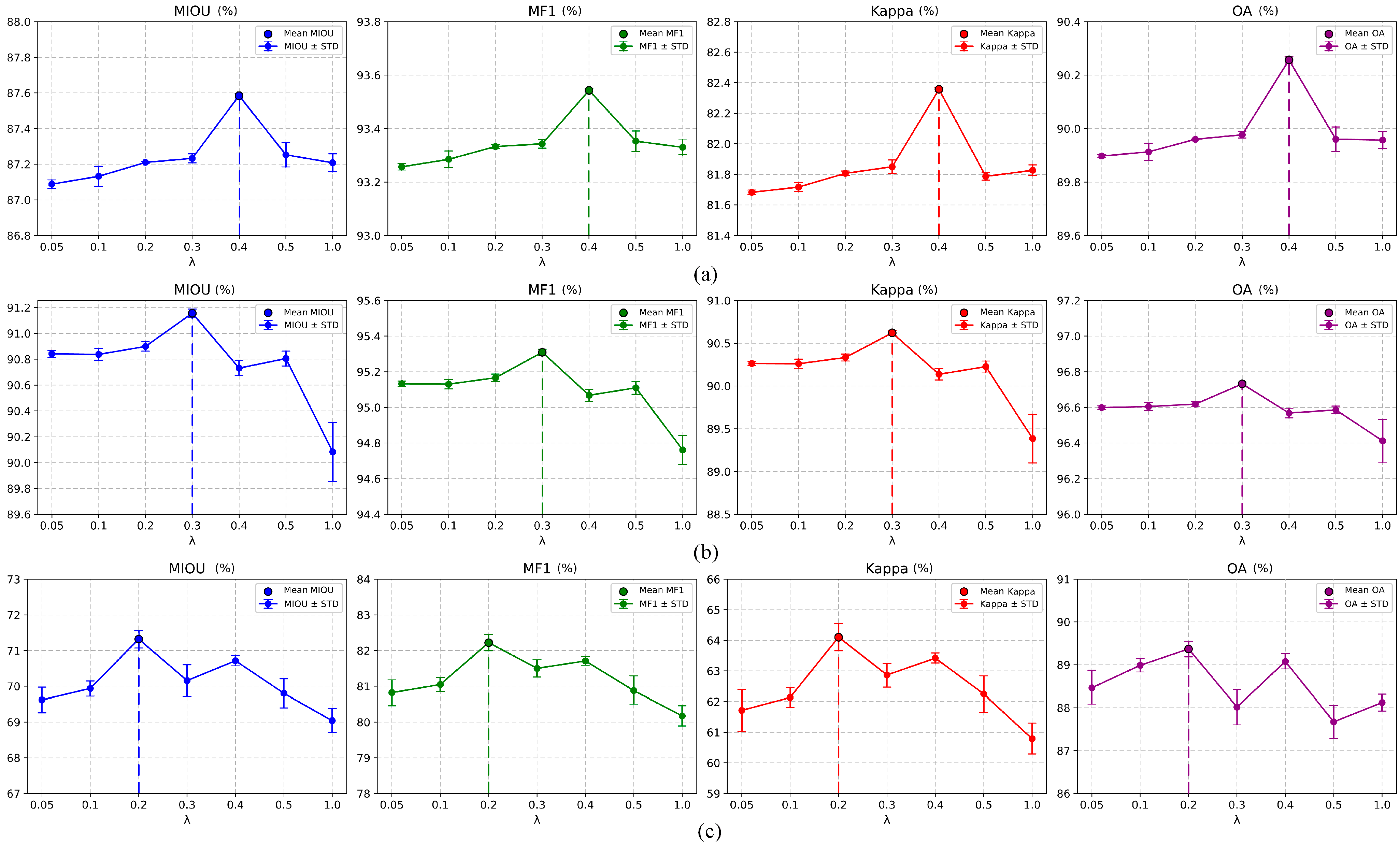
To investigate the influence of different λ values on model performance, each λ experiment was independently repeated three times, and the mean and standard deviation of MIoU, MF1, Kappa, and OA were reported.

The variations in these metrics with respect to λ are summarized in Figure 10, where the error bars denote the standard deviation across trials, providing a measure of performance stability. Figure 10a–c indicate that the optimal λ values are 0.4, 0.3, and 0.2 for the GID-CD, JY-CD, and QX-CD datasets, respectively. By synthesizing the boundary complexity distributions in Figure 8 with the segmentation performance variations under different λ values in Figure 10, a clear negative correlation can be observed—datasets with higher boundary tortuosity tend to achieve optimal performance at smaller λ values. For example, QX-CD exhibits the highest mean tortuosity, reflecting more fragmented and geometrically complex boundaries, and correspondingly achieves optimal performance at λ = 0.2. In contrast, GID-CD and JY-CD have relatively lower boundary complexity and perform best at larger λ values (0.4 and 0.3, respectively).

In summary, the optimal value of the boundary weight λ varies across different terrain types. For datasets with clear and regular boundaries, such as GID-CD and JY-CD, the model exhibits relatively stable performance when λ ranges from 0.2 to 0.5. However, in the mountainous QX-CD dataset, which is characterized by blurry boundaries and complex geometries, performance metrics fluctuate significantly with changes in λ, indicating that fragmented boundaries are more sensitive to boundary supervision. In this case, a smaller λ achieves better results. Overall, all three datasets exhibit a common trend where accuracy initially improves with increasing λ, reaches a peak, and then gradually declines. This suggests that overly strong boundary supervision may interfere with region-level semantic representation in the segmentation branch, particularly in terrain with ambiguous or inconsistently labeled boundaries. In such cases, the model benefits more from semantic features directly extracted from the image, rather than from boundary priors that may reflect human annotation preferences. Therefore, boundary weighting should be carefully balanced to harmonize semantic region representation and edge guidance.

5.2. Ablation Study

To verify the effectiveness of SAM-SANet, ablation experiments were conducted on the three datasets with the aim of assessing the specific impact of each module to the overall segmentation performance. The ablation mainly focused on the SAB, the SAM branch that perceives cropland boundaries (BCB_SAM), and the BFFM and PGSM incorporated to enhance cropland boundary representation. For the BFFM and PGSM in particular, a more fine-grained ablation was performed. In addition to the cumulative ablation setting, the parameters of either BFFM or PGSM were frozen during training, while the remaining network components were kept trainable. By freezing BFFM, the PGSM branch remains learnable, and the performance difference reflects the independent contribution of BFFM. By freezing PGSM, the BFFM branch remains learnable, and the performance difference reflects the independent contribution of PGSM. This strategy preserves the original network architecture, avoids side effects caused by physically removing modules, and isolates the effect of BFFM and PGSM by quantifying the performance change when their learning ability is disabled.

All ablation settings adopt the optimal λ values identified in the sensitivity analysis of Section 5.1 to ensure consistency across comparisons. The results of the effect of each component on the segmentation performance are shown in

Table 4. Ablation study on GID-CD. All evaluation metrics are presented in percentage format (%). The values in parentheses indicate the accuracy improvements achieved over the SAB alone.

SAB	BCBSAM			Cropland-IOU/F1	Non-Cropland-IOU/F1	MIOU	MF1	Kappa	OA
	PEA	PGSM	BFFM
✓				88.64/93.98	84.95/91.86	86.79	92.92	81.39	89.56
✓	✓			88.72/94.02	85.16/91.98	86.94 (+0.15)	93.00 (+0.08)	81.46 (+0.07)	89.62 (+0.06)
✓	✓	✓		88.97/94.34	85.00/92.06	86.99 (+0.20)	93.20 (+0.28)	81.58 (+0.19)	89.67 (+0.11)
✓	✓		✓	89.12/94.43	85.51/92.36	87.32 (+0.53)	93.40 (+0.48)	81.99 (+0.60)	89.93 (+0.37)
✓	✓	✓	✓	89.31/94.53	85.85/92.55	87.58 (+0.79)	93.54 (+0.62)	82.37 (+0.98)	90.25 (+0.69)

,

Table 5. Ablation study on JY-CD. All evaluation metrics are presented in percentage format (%). The values in parentheses indicate the accuracy improvements achieved over the SAB alone.

SAB	BCB			Cropland-IOU/F1	Non-Cropland-IOU/F1	MIOU	MF1	Kappa	OA
	PEA	PGSM	BFFM
✓				95.61/97.75	85.60/92.24	90.60	94.98	90.01	96.22
✓	✓			95.59/97.75	85.63/92.26	90.61 (+0.01)	95.01 (+0.03)	90.12 (+0.11)	96.51 (+0.29)
✓	✓	✓		95.68/97.79	85.72/92.31	90.70 (+0.10)	95.05 (+0.07)	90.10 (+0.09)	96.57 (+0.35)
✓	✓		✓	95.81/97.86	86.32/92.66	91.07 (+0.47)	95.26 (+0.28)	90.52 (+0.51)	96.69 (+0.47)
✓	✓	✓	✓	95.88/97.96	86.47/92.74	91.17 (+0.57)	95.35 (+0.37)	90.74 (+0.73)	96.78 (+0.56)

and

Table 6. Ablation study on QX-CD. All evaluation metrics are presented in percentage format (%). The values in parentheses indicate the accuracy improvements achieved over the SAB alone.

SAB	BCB			Cropland-IOU/F1	Non-Cropland-IOU/F1	MIOU	MF1	Kappa	OA
	PEA	PGSM	BFFM
✓				52.87/69.17	87.15/93.13	70.01	81.15	62.31	88.77
✓	✓			54.13/70.24	87.53/93.35	70.83 (+0.82)	81.79 (+0.64)	63.61 (+1.30)	89.14 (+0.37)
✓	✓	✓		54.23/70.33	87.32/93.25	70.77 (+0.76)	81.79 (+0.64)	63.53 (+1.22)	88.98 (+0.21)
✓	✓		✓	54.47/70.52	87.82/93.45	71.15 (+1.14)	81.99 (+0.84)	63.99 (+1.68)	89.34 (+0.57)
✓	✓	✓	✓	54.81/70.81	87.97/93.60	71.39 (+1.38)	82.21 (+1.06)	64.14 (+1.83)	89.49 (+0.72)

. The values in parentheses indicate the performance improvement compared to the SAB baseline.

5.2.1. Synergistic Effect of SAB and BCB

The introduction of the BCB_SAM branch results in consistent, performance gains across all three datasets, suggesting the beneficial effect of boundary supervision on the model’s structural representation. Compared to the results of the model with only the SAB, the metrics on the GID-CD show that mIoU increased from 86.79% to 86.94% (+0.15 pp), with mF1 and Kappa improving by +0.08 and +0.07 pp, respectively. These results indicate that BCB_SAM improved the model’s ability to preserve the spatial coherence and shape consistency of large-scale cropland boundaries. On JY-CD, the addition of BCB_SAM yielded an mIoU gain of +0.01 pp and mF1 of +0.03 pp, with Kappa and OA increasing by +0.11 pp and +0.29, respectively. Although the performance gains were modest on JY-CD, they are still meaningful given the regular and contiguous nature of cropland boundaries in flat terrain. This indicates that the BCB_SAM primarily serves to enhance the SAB by refining fine-grained edge details and correcting minor boundary localization errors. On the QX-CD mountainous dataset, the improvements are more substantial: mIoU is increased by +0.82 pp, mF1 by +0.64 pp, and Kappa by +1.30 pp, OA by +0.37%, demonstrating BCB_SAM ’s improved capability in capturing irregular and fragmented cropland boundaries. This enhancement mitigates common issues such as broken or blurred boundaries effectively in terraced landscapes.

Overall, incorporating the BCB_SAM in parallel with SAB improves the edge localization outcomes substantially and compensates for SAB’s limitations in capturing fine-grained boundary details—particularly in rugged or low-contrast environments.

5.2.2. Effectiveness of BFFM and PGSM

To further isolate the independent contributions of BFFM and PGSM, complementary experiments were conducted by freezing the parameters of one module at a time while keeping the other trainable. The results reveal that both BFFM-only and PGSM-only settings outperform the configuration without either module, yet remain inferior to the fully trainable combination. By further integrating BFFM and PGSM into the BCB_SAM branch, the model achieves substantial performance gains across all datasets, validating the importance of boundary-aware feature fusion and prompt-driven guidance in boundary modeling. On the GID-CD dataset, compared to the BCB_SAM branch, mIoU increased by +0.64 pp, mF1 by +0.54 pp, Kappa by +0.91 pp, and OA by +0.63 pp. This indicates that BFFM strengthens the aggregation of multi-level boundary features under large-scale scenarios, while PGSM guides the model to focus on critical boundary regions through appropriate prompts, thereby achieving more accurate object localization and refined boundary reconstruction. On the JY-CD dataset, mIoU improved from 90.61% to 91.17% (+0.56 pp), mF1 by +0.34 pp, Kappa by +0.62 pp, and OA by +0.27 pp. BFFM compensated for the ViT encoder’s limited local boundary detail extraction capability by aggregating multi-scale edge features, while PGSM reinforced boundary localization by concentrating on uncertain boundary zones, enhancing boundary closure and continuity. On the QX-CD mountainous dataset, the effect was even more significant: mIoU, mF1, Kappa and OA increased by +0.56 pp, +0.42 pp, +1.53 pp and +0.35 pp, respectively. These results indicate that BFFM provided robust structural continuity under complex terrains, and that the PGSM generated effective sparse prompts to guide the model in correcting broken or curved edges, leading to refined segmentation along irregular boundaries.

By visualizing the intermediate feature maps of the BFFM and PGSM (as shown in Figure 11), distinct activation patterns emerge across different stages of feature processing. The shallow feature maps (F_shallow), derived from early layers of the backbone, primarily capture low-level spatial structures such as textures and color variations, often exhibiting noisy and disordered responses. As the features deepen (F_deep), the feature representations become more semantically enriched, revealing clearer object contours and structural patterns. The fused feature map from the BFFM (F_BFFM) exhibits enhanced activation along object boundaries, highlights boundary regions more prominently. In the PGSM, these boundary-focused fused features are further refined to generate the final prompt-related feature map (F_PGSM), where high-response regions are densely concentrated in the foreground. These salient activations are subsequently transformed into sparse prompt boxes, which guide the input to the SAM mask decoder.

In conclusion, the joint use of BFFM and PGSM guided the model to focus on critical boundaries effectively, improving both structural awareness and prompt responsiveness. This synergy significantly enhanced boundary representation quality and overall robustness in diverse and challenging cropland landscapes.

5.2.3. Effectiveness of the PEA

To further evaluate the practical effectiveness of the proposed PEA module, a comparative experiment was conducted on the JY-CD dataset. Specifically, the full SAM-SANet model (SAB+BCB_{SAM+PEA+BFFM+PGSM}) integrating the PEA module was compared with its counterpart without the PEA module (SAB+BCB_{SAM+BFFM+PGSM}). As presented in

Table 7. Impact of the PEA module on SAM-SANet performance and efficiency.

Model	Input_Size	MIOU (%)	MF1 (%)	Params (M)	GFLOPs
SAB+BCBSAM+BFFM+PGSM	1024 × 1024	90.10	94.71	106.95	3524.08
SAB+BCBSAM+PEA+BFFM+PGSM	256 × 256	91.17	95.35	106.95	303.22

, the PEA-enabled SAM-SANet achieves comparable segmentation accuracy while substantially reducing computational cost (in terms of GFLOPs), without introducing additional model parameters. The results highlight the critical role of the PEA module in enabling support for smaller input sizes (256 × 256), thereby improving facilitating practical deployment.

5.3. Running Efficiency

To further evaluate the computational efficiency of the proposed method, we compared different model configurations in terms of computational cost and model size. Specifically, we analyze the impact of each module, including the semantically aware branch (SAB), the boundary-constrained branch based on SAM (BCB), the position embedding adapter (PEA), as well as the BFFM and PGSM, on the overall resource consumption.

As shown in

Table 8. Comparison of different model parameters and computational efficiency.

SAB	BCB	PEA	BFFM+PGSM	Params (M)	GFLOPs
✓				11.68	23.48
	✓			90.35	2976.10
✓	✓			102.03	3351.74
✓	✓	✓		102.03	281.95
✓	✓	✓	✓	106.95	303.22

, the SAB is lightweight with low parameter count and computational cost. In contrast, the original SAM branch (BCB) has high computational cost due to its Vit backbone and large input size. Incorporating the PEA module enables SAM to process 256 × 256 inputs, which substantially reduces the computational cost. Adding BFFM and PGSM introduces only slight overhead while providing moderate improvements in segmentation accuracy. Overall, the full model maintains a good balance between accuracy and efficiency, making it suitable for practical deployment.

6. Conclusions

In this study, the challenges of cropland extraction accuracy and boundary preservation in high-resolution remote sensing imagery were addressed through the proposal of a novel dual-branch network architecture named SAM-SANet. The objective is to jointly enhance semantic perception and boundary refinement for cropland extraction under complex terrain conditions, where field shapes may be irregular, boundaries are often blurred, and class confusion is prevalent. Specifically, SAM-SANet integrates a semantically aware branch (SAB)and a boundary-constrained SAM branch (BCB) to handle region-level semantic recognition and contour-level boundary modeling separately. These two branches are jointly optimized through a combination of segmentation and boundary loss functions to achieve collaborative learning between regional semantics and edge precision. To improve SAM’s adaptability and representational power in RS scenarios, the boundary branch incorporates three key modules: The PEA addresses the incompatibility between SAM’s fixed input size and the dimensions of cropland images, thereby enhancing spatial alignment and the expressiveness of positional embeddings. The BFFM and the PGSM jointly enhance the accuracy of prompt-driven segmentation for complex cropland boundary representation by aggregating multi-scale edge features and generating prompt embeddings associated with cropland boundaries. In extensive experiments and ablation studies conducted on three RS cropland datasets, each with distinct topographical characteristics, SAM-SANet achieved superior performance in preserving cropland integrity, ensuring boundary clarity, and maintaining spatial consistency. Overall, the proposed model outperformed existing mainstream methods across multiple evaluation metrics.

Despite its promising performance, SAM-SANet still faces certain limitations in its effectively integration of semantic and boundary information under complex agricultural landscapes. In particular, scenarios involving fragmented plots or small irregular fields reveal localized inconsistencies between branches, highlighting the need for improved joint modeling strategies. Future research will focus on two key directions: (1) exploring deep collaborative optimization between the prompt mechanism and semantic–boundary feature fusion to improve the model’s ability to diverse cropland morphologies and (2) incorporating multi-temporal RS data to better capture seasonal variations and crop rotation patterns, thereby improving the model’s capability and practical applicability in high-resolution cropland extraction.

References

1. Fei, L.; Shuang, M.; Xiaolin, L. Changing multi-scale spatiotemporal patterns in food security risk in China. J. Clean. Prod. 2023, 384, 135618. [Google Scholar] [CrossRef]
2. Li, Y.; Liu, W.; Feng, Q.; Zhu, M.; Yang, L.; Zhang, J.; Yin, X. The role of land use change in affecting ecosystem services and the ecological security pattern of the Hexi Regions, Northwest China. Sci. Total Environ. 2023, 855, 158940. [Google Scholar] [CrossRef]
3. Castaldi, F.; Halil Koparan, M.; Wetterlind, J.; Žydelis, R.; Vinci, I.; Özge Savaş, A.; Kıvrak, C.; Tunçay, T.; Volungevičius, J.; Obber, S.; et al. Assessing the capability of Sentinel-2 time-series to estimate soil organic carbon and clay content at local scale in croplands. ISPRS J. Photogramm. Remote Sens. 2023, 199, 40–60. [Google Scholar] [CrossRef]
4. Huang, X.; Reba, M.; Coffin, A.; Runkle, B.R.K.; Huang, Y.; Chapman, B.; Ziniti, B.; Skakun, S.; Kraatz, S.; Siqueira, P.; et al. Cropland mapping with L-band UAVSAR and development of NISAR products. Remote Sens. Environ. 2021, 253, 112180. [Google Scholar] [CrossRef]
5. Zhang, D.; Pan, Y.; Zhang, J.; Hu, T.; Zhao, J.; Li, N.; Chen, Q. A generalized approach based on convolutional neural networks for large area cropland mapping at very high resolution. Remote Sens. Environ. 2020, 247, 111912. [Google Scholar] [CrossRef]
6. Zhang, W.; Qie, R. Spatiotemporal change of cultivated land in China during 2000–2020. PLoS ONE 2024, 19, e0293082. [Google Scholar] [CrossRef]
7. Yang, G.; Li, X.; Liu, P.; Yao, X.; Zhu, Y.; Cao, W.; Cheng, T. Automated in-season mapping of winter wheat in China with training data generation and model transfer. ISPRS J. Photogramm. Remote Sens. 2023, 202, 422–438. [Google Scholar] [CrossRef]
8. Waldner, F.; Canto, G.S.; Defourny, P. Automated annual cropland mapping using knowledge-based temporal features. ISPRS J. Photogramm. Remote Sens. 2015, 110, 1–13. [Google Scholar] [CrossRef]
9. Zhang, W.; Guo, S.; Zhang, P.; Xia, Z.; Zhang, X.; Lin, C.; Tang, P.; Fang, H.; Du, P. A Novel Knowledge-Driven Automated Solution for High-Resolution Cropland Extraction by Cross-Scale Sample Transfer. IEEE Trans. Geosci. Remote Sens. 2023, 61, 4406816. [Google Scholar] [CrossRef]
10. Bruzzone, L.; Carlin, L. A Multilevel Context-Based System for Classification of Very High Spatial Resolution Images. IEEE Trans. Geosci. Remote Sens. 2006, 44, 2587–2600. [Google Scholar] [CrossRef]
11. Graesser, J.; Ramankutty, N. Detection of cropland field parcels from Landsat imagery. Remote Sens. Environ. 2017, 201, 165–180. [Google Scholar] [CrossRef]
12. Johansen, K.; Lopez, O.; Tu, Y.-H.; Li, T.; McCabe, M.F. Center pivot field delineation and mapping: A satellite-driven object-based image analysis approach for national scale accounting. ISPRS J. Photogramm. Remote Sens. 2021, 175, 1–19. [Google Scholar] [CrossRef]
13. Cai, Z.; Hu, Q.; Zhang, X.; Yang, J.; Wei, H.; He, Z.; Song, Q.; Wang, C.; Yin, G.; Xu, B. An Adaptive Image Segmentation Method with Automatic Selection of Optimal Scale for Extracting Cropland Parcels in Smallholder Farming Systems. Remote Sens. 2022, 14, 3067. [Google Scholar] [CrossRef]
14. Lu, H.; Liu, C.; Li, N.; Fu, X.; Li, L. Optimal segmentation scale selection and evaluation of cultivated land objects based on high-resolution remote sensing images with spectral and texture features. Environ. Sci. Pollut. Res. Int. 2021, 28, 27067–27083. [Google Scholar] [CrossRef] [PubMed]
15. Cheng, T.; Ji, X.; Yang, G.; Zheng, H.; Ma, J.; Yao, X.; Zhu, Y.; Cao, W. DESTIN: A new method for delineating the boundaries of crop fields by fusing spatial and temporal information from WorldView and Planet satellite imagery. Comput. Electron. Agric. 2020, 178, 105787. [Google Scholar] [CrossRef]
16. Wagner, M.P.; Oppelt, N. Extracting Agricultural Fields from Remote Sensing Imagery Using Graph-Based Growing Contours. Remote Sens. 2020, 12, 1205. [Google Scholar] [CrossRef]
17. Tetteh, G.O.; Gocht, A.; Conrad, C. Optimal parameters for delineating agricultural parcels from satellite images based on supervised Bayesian optimization. Comput. Electron. Agric. 2020, 178, 105696. [Google Scholar] [CrossRef]
18. Li, J.; Wei, Y.; Wei, T.; He, W. A Comprehensive Deep-Learning Framework for Fine-Grained Farmland Mapping from High-Resolution Images. IEEE Trans. Geosci. Remote Sens. 2025, 63, 5601215. [Google Scholar] [CrossRef]
19. Ronneberger, O.; Fischer, P.; Brox, T. U-Net: Convolutional Networks for Biomedical Image Segmentation. In Proceedings of the International Conference on Medical Image Computing and Computer-Assisted Intervention (MICCAI), Munich, Germany, 5–9 October 2015; pp. 234–241. [Google Scholar]
20. Chen, L.-C.; Zhu, Y.; Papandreou, G.; Schroff, F.; Adam, H. Encoder-Decoder with Atrous Separable Convolution for Semantic Image Segmentation. In Proceedings of the European Conference on Computer Vision (ECCV), Munich, Germany, 8–14 September 2018; pp. 833–851. [Google Scholar]
21. Dosovitskiy, A.; Beyer, L.; Kolesnikov, A.; Weissenborn, D.; Zhai, X.; Unterthiner, T.; Dehghani, M.; Minderer, M.; Heigold, G.; Gelly, S.; et al. An Image is Worth 16×16 Words: Transformers for Image Recognition at Scale. arXiv 2020, arXiv:2010.11929. [Google Scholar] [CrossRef]
22. Zheng, S.; Lu, J.; Zhao, H.; Zhu, X.; Luo, Z.; Wang, Y.; Fu, Y.; Feng, J.; Xiang, T.; Torr, P.H.S.; et al. Rethinking Semantic Segmentation from a Sequence-to-Sequence Perspective with Transformers. In Proceedings of the 2021 IEEE/CVF Conference on Computer Vision and Pattern Recognition (CVPR), Nashville, TN, USA, 20–25 June 2021; pp. 6877–6886. [Google Scholar] [CrossRef]
23. Wang, L.; Li, R.; Zhang, C.; Fang, S.; Duan, C.; Meng, X.; Atkinson, P.M. UNetFormer: A UNet-like transformer for efficient semantic segmentation of remote sensing urban scene imagery. ISPRS J. Photogramm. Remote Sens. 2022, 190, 196–214. [Google Scholar] [CrossRef]
24. Wu, H.; Huang, P.; Zhang, M.; Tang, W.; Yu, X. CMTFNet: CNN and Multiscale Transformer Fusion Network for Remote-Sensing Image Semantic Segmentation. IEEE Trans. Geosci. Remote Sens. 2023, 61, 2004612. [Google Scholar] [CrossRef]
25. Kirillov, A.; Mintun, E.; Ravi, N.; Mao, H.; Rolland, C.; Gustafson, L.; Xiao, T.; Whitehead, S.; Berg, A.C.; Lo, W.-Y.; et al. Segment Anything. In Proceedings of the IEEE/CVF International Conference on Computer Vision (ICCV 2023), Paris, France, 1–6 October 2023; IEEE: New York, NY, USA, 2023; pp. 4015–4026. [Google Scholar] [CrossRef]
26. Sun, H.; Wei, Z.; Yu, W.; Yang, G.; She, J.; Zheng, H.; Jiang, C.; Yao, X.; Zhu, Y.; Cao, W.; et al. SIDEST: A sample-free framework for crop field boundary delineation by integrating super-resolution image reconstruction and dual edge-corrected Segment Anything model. Comput. Electron. Agric. 2025, 230, 109897. [Google Scholar] [CrossRef]
27. Ma, X.; Wu, Q.; Zhao, X.; Zhang, X.; Pun, M.-O.; Huang, B. SAM-Assisted Remote Sensing Imagery Semantic Segmentation with Object and Boundary Constraints. IEEE Trans. Geosci. Remote Sens. 2024, 62, 5636916. [Google Scholar] [CrossRef]
28. Lin, X.; Xiang, Y.; Zhang, L.; Yang, X.; Yan, Z.; Yu, L. SAMUS: Adapting Segment Anything Model for Clinically-Friendly and Generalizable Ultrasound Image Segmentation. arXiv 2023, arXiv:2309.06824. [Google Scholar] [CrossRef]
29. Chen, K.; Liu, C.; Chen, H.; Zhang, H.; Li, W.; Zou, Z.; Shi, Z. RSPrompter: Learning to Prompt for Remote Sensing Instance Segmentation Based on Visual Foundation Model. IEEE Trans. Geosci. Remote Sens. 2024, 62, 4701117. [Google Scholar] [CrossRef]
30. Luo, M.; Zhang, T.; Wei, S.; Ji, S. SAM-RSIS: Progressively Adapting SAM With Box Prompting to Remote Sensing Image Instance Segmentation. IEEE Trans. Geosci. Remote Sens. 2024, 62, 4413814. [Google Scholar] [CrossRef]
31. Sultan, R.I.; Li, C.; Zhu, H.; Khanduri, P.; Brocanelli, M.; Zhu, D. GeoSAM: Fine-Tuning SAM with Sparse and Dense Visual Prompting for Automated Segmentation of Mobility Infrastructure. arXiv 2023, arXiv:2311.11319. [Google Scholar] [CrossRef]
32. Wang, C.; Chen, J.; Meng, Y.; Deng, Y.; Li, K.; Kong, Y. SAMPolyBuild: Adapting the Segment Anything Model for polygonal building extraction. ISPRS J. Photogramm. Remote Sens. 2024, 218, 707–720. [Google Scholar] [CrossRef]
33. Chen, Y.; Zhou, J.; Chen, Y.; Wang, J.; Zhang, X.; Ge, Y.; Ma, H. Edge-enhanced SAM for extracting photovoltaic power plants from remote sensing imagery. Int. J. Appl. Earth Obs. Geoinf. 2025, 140, 104580. [Google Scholar] [CrossRef]
34. Ma, X.; Zhang, X.; Pun, M.-O.; Huang, B. A Unified Framework with Multimodal Fine-Tuning for Remote Sensing Semantic Segmentation. IEEE Trans. Geosci. Remote Sens. 2025, 63, 5405015. [Google Scholar] [CrossRef]
35. Kato, S.; Mitsuoka, H.; Hotta, K. Generalized SAM: Efficient Fine-Tuning of SAM for Variable Input Image Sizes. In Proceedings of the European Conference on Computer Vision (ECCV) Workshops, Milan, Italy, 29 September–4 October 2024; Lecture Notes in Computer Science. Springer: Cham, Switzerland, 2025; Volume 15633. [Google Scholar] [CrossRef]
36. Tong, X.-Y.; Xia, G.-S.; Lu, Q.; Shen, H.; Li, S.; You, S.; Zhang, L. Land-cover classification with high-resolution remote sensing images using transferable deep models. Remote Sens. Environ. 2020, 237, 111322. [Google Scholar] [CrossRef]
37. Tai, A.; Huang, W.; Xu, D.; Lou, Y.; Hu, J.; He, Q. A Deep Learning Framework for Boundary-Aware Semantic Segmentation. In Proceedings of the 2025 5th International Conference on Artificial Intelligence and Industrial Technology Applications (AIITA), Xi’an, China, 28–30 March 2025; IEEE: New York, NY, USA, 2025. [Google Scholar] [CrossRef]
38. Liu, J.; Gu, H.; Li, Z.; Chen, H.; Chen, H. Multi-Scale Feature Fusion Attention Network for Building Extraction in Remote Sensing Images. Electronics 2024, 13, 923. [Google Scholar] [CrossRef]
39. Girshick, R. Fast R-CNN. In Proceedings of the IEEE International Conference on Computer Vision (ICCV), Santiago, Chile, 7–13 December 2015; pp. 1440–1448. [Google Scholar] [CrossRef]
40. He, K.; Gkioxari, G.; Dollar, P.; Girshick, R. Mask R-CNN. In Proceedings of the IEEE International Conference on Computer Vision (ICCV), Venice, Italy, 22–29 October 2017; pp. 2961–2969. [Google Scholar] [CrossRef]
41. Yin, B.W.; Cao, J.L.; Cheng, M.M.; Hou, Q. DFormerv2: Geometry Self-Attention for RGB-D Semantic Segmentation. In Proceedings of the IEEE/CVF Conference on Computer Vision and Pattern Recognition (CVPR), Nashville, TN, USA, 10–17 June 2025. [Google Scholar] [CrossRef]
42. Zhao, C.; Li, Y.; Weng, M. A Fractal Approach to Urban Boundary Delineation Based on Raster Land Use Maps: A Case of Shanghai, China. Land 2021, 10, 941. [Google Scholar] [CrossRef]
43. Fu, J.; Thomas, H.R.; Li, C. Tortuosity of porous media: Image analysis and physical simulation. Earth-Sci. Rev. 2021, 212, 103439. [Google Scholar] [CrossRef]
44. Wang, W.; Jiao, L.; Zhang, W.; Jia, Q.; Su, F.; Xu, G.; Ma, S. Delineating urban growth boundaries under multi-objective and constraints. Sustain. Cities Soc. 2020, 61, 102279. [Google Scholar] [CrossRef]
45. Ge, J.; Zhang, H.; Zuo, L.; Xu, L.; Jiang, J.; Song, M.; Ding, Y.; Xie, Y.; Wu, F.; Wang, C.; et al. Large-scale rice mapping under spatiotemporal heterogeneity using multi-temporal SAR images and explainable deep learning. ISPRS J. Photogramm. Remote Sens. 2025, 220, 395–412. [Google Scholar] [CrossRef]
Figure 1. Maps of the two study areas: (a1) Juye (1 April 2016) and (b1) Qixia (22 August 2016). Each study area is divided into training (black), validation (cyan), and test (red) areas. (a1,b1) show the GF-1 satellite images for Juye and Qixia, respectively, while (a2,b2) show the corresponding ground truth results of cropland in the two study areas.
Remotesensing 17 03424 g001
Figure 2. Sample display diagram of a portion of the dataset.
Remotesensing 17 03424 g002
Figure 3. Network architecture of SAM-SANet. (a) The overall dual-branch framework consists of a semantically aware branch (SAB) and a boundary-constrained branch (BCB), in which modules labeled as “Frozen” have their parameters fixed to retain pre-trained features. “PEA” is the position embedding adapter. (b) Boundary-aware feature fusion module (BFFM). (c) Prompt generation and selection module (PGSM).
Remotesensing 17 03424 g003
Figure 4. High-resolution cropland extraction results of different models on GID-CD. The yellow and blue boxes indicate regions where differences among models are most visually significant. Subfigures (ad) show four representative regions with varying boundary complexity, texture patterns, and background interference.
Remotesensing 17 03424 g004
Figure 5. High-resolution cropland extraction results of different models on JY-CD. The yellow and blue boxes indicate regions where differences among models are most visually significant. Subfigures (ad) show four representative JY-CD regions with different boundary characteristics.
Remotesensing 17 03424 g005
Figure 6. High-resolution cropland extraction results of different models on QX-CD. The yellow and blue boxes indicate regions where differences among models are most visually significant. Subfigures (ad) show four representative QX-CD regions with complex terrain, irregular parcel boundaries, and strong texture variation.
Remotesensing 17 03424 g006
Figure 7. Performance of the proposed method under different area thresholds across the GID-CD, JY-CD, and QX-CD datasets. Subfigures (ac) correspond to the GID-CD, JY-CD, and QX-CD datasets, respectively.
Remotesensing 17 03424 g007
Figure 8. Histogram-based distributions of cropland boundary tortuosity for the GID-CD, JY-CD, and QX-CD datasets.
Remotesensing 17 03424 g008
Figure 9. Violin plots of cropland boundary tortuosity for the GID-CD, JY-CD, and QX-CD datasets.
Remotesensing 17 03424 g009
Figure 10. Boundary sensitivity analysis on the three datasets. Subfigures (ac) correspond to the results on GID-CD, JY-CD, and QX-CD, respectively, showing the impact of different λ values on MIoU, MF1, Kappa, and OA.
Remotesensing 17 03424 g010
Figure 11. Visualization of intermediate feature maps in the BFFM and PGSM. Warmer colors (red/yellow) indicate higher activation responses, while cooler colors (blue) denote lower responses.
Remotesensing 17 03424 g011