Next-Generation Drought Forecasting: Hybrid AI Models for Climate Resilience

Highlights

What are the main findings?

• A hybrid Random Forest-LSTM model improves drought forecasting by using RF to identify the most critical climate predictors and LSTM to model their temporal evolution.
• The Yellow River Basin is projected to face a rapid intensification of drought severity and frequency post-2040, especially under the high-emission SSP5-8.5 climate scenario.

What is the implication of the main finding?

• The hybrid AI approach provides a powerful and replicable framework for developing more reliable seasonal and long-term drought early warning systems.
• The findings directly support anticipatory water resource management by quantifying future drought risks and informing climate adaptation strategies in critical water-scarce regions.

Abstract

Droughts are increasingly threatening ecological balance, agricultural productivity, and socio-economic resilience—especially in semi-arid regions like the Inner Mongolia segment of China’s Yellow River Basin. This study presents a hybrid drought forecasting framework integrating machine learning (ML) and deep learning (DL) models with high-resolution historical and downscaled future climate data. TerraClimate observations (1985–2014) and bias-corrected CMIP6 projections (2030–2050) under SSP2-4.5 and SSP5-8.5 scenarios were utilized to develop and evaluate the models. Among the tested ML algorithms, Random Forest (RF) demonstrated the best trade-off between accuracy and interpretability and was selected for feature importance analysis. The top-ranked predictors—precipitation, solar radiation, and maximum temperature—were used to train a Long Short-Term Memory (LSTM) network. The LSTM outperformed all ML models, achieving high predictive skill (R² = 0.766, CC = 0.880, RMSE = 0.885). Scenario-based projections revealed increasing drought severity and variability under SSP5-8.5, with mean PDSI values dropping below −3 after 2040 and deepening toward −4 by 2049. The high-emission scenario also exhibited broader uncertainty bands and amplified interannual anomalies. These findings highlight the value of hybrid AI–climate modeling approaches in capturing complex drought dynamics and supporting anticipatory water resource planning in vulnerable dryland environments.

1. Introduction

Drought is increasingly recognized as one of the most destructive and pervasive environmental hazards worldwide. It affects ecological balance, agricultural production, freshwater availability, and socio-economic resilience [1,2]. Unlike rapid-onset disasters such as floods or hurricanes, drought develops slowly but affects vast regions extensively, making it especially challenging to monitor, predict, and manage [3]. In the context of accelerating climate change, drought events have become more frequent, prolonged, and intense, driven by rising global temperatures and increasingly erratic precipitation patterns [4,5]. Anthropogenic warming has amplified the likelihood and severity of compound dry-heat extremes, posing serious threats to ecosystems and communities [1,6]. Dryland regions such as Inner Mongolia in the Yellow River Basin of China are particularly vulnerable due to their fragile ecosystems and dependence on rainfall for agriculture and water supply. Studies have shown that this region exhibits high drought frequency, making it imperative to develop accurate and timely forecasting tools to mitigate impacts and support sustainable resource management [7]. Traditional drought forecasting methods often rely on statistical correlations or physically based hydrological models. While these methods have laid a strong foundation, they struggle to fully capture the complex, non-linear interactions among atmospheric variables, land surface processes, and human influences [8,9]. Moreover, many conventional models are limited by their dependency on historical calibration, which reduces their effectiveness under novel climate conditions outside the training range [7]. Widely used drought indices such as the Palmer Drought Severity Index (PDSI) or Standardized Precipitation Index (SPI) often fail to reflect changes in evapotranspiration dynamics or heatwave intensities, leading to biased assessments under warming scenarios [10].

These limitations have led to a growing interest in artificial intelligence (AI) and machine learning (ML) approaches for drought prediction. AI-based models—particularly those based on ensemble learning (e.g., Random Forest, XGBoost, and Gradient Boosting) and deep learning architectures such as Long Short-Term Memory (LSTM) networks—have demonstrated superior capabilities in modeling non-linear and lagged dependencies in climate and hydrological data [11,12]. Unlike static regression models, AI techniques can flexibly learn from multi-dimensional, high-volume datasets and adapt to changing conditions. For instance, LSTM models have been shown to outperform traditional statistical methods in predicting drought indices over various lead times [13,14]. In addition to algorithmic advances, the increasing availability of high-resolution climate and remote sensing data has significantly enhanced the potential for accurate drought modeling. The NASA Earth Exchange Global Daily Downscaled Projection (NEX-GDDP) dataset, for example, provides bias-corrected, spatially detailed projections under CMIP6 scenarios such as SSP2-4.5 (Shared Socio-economic Pathway 2—moderate mitigation) and SSP5-8.5 (high-emission baseline) [15,16]. These projections, when integrated with satellite-derived variables such as NDVI, land surface temperature, and soil moisture (e.g., from GRACE or MODIS), enable precise analysis of spatiotemporal drought dynamics [17,18]. The advent of cloud-based platforms like Google Earth Engine has further streamlined access, integration, and processing of such diverse datasets, allowing the development of high-resolution, scalable drought models [18]. Despite these opportunities, existing operational drought forecasting models often underutilize the synergy of high-resolution data and hybrid AI methods. In many studies, a single modeling technique or limited data sources are still employed, which diminishes predictive performance and increases uncertainty.

Purely data-driven models may suffer from overfitting and lack physical interpretability, while mechanistic models may not adequately capture nonlinearity and variable interactions [13]. This motivates hybrid models that exploit the strengths of both approaches. A notable example is the hybrid Random Forest–LSTM architecture, in which the Random Forest model filters and ranks critical hydro-climatic features. LSTM subsequently models their temporal behavior to predict drought indices [14]. Such frameworks have improved accuracy and interpretability while effectively addressing temporal dependencies in drought development. Another approach by Vo et al. [13] integrates LSTM networks with climate model outputs, resulting in superior generalization across diverse scenarios. These studies underscore the promise of hybrid AI models in advancing drought early warning systems.

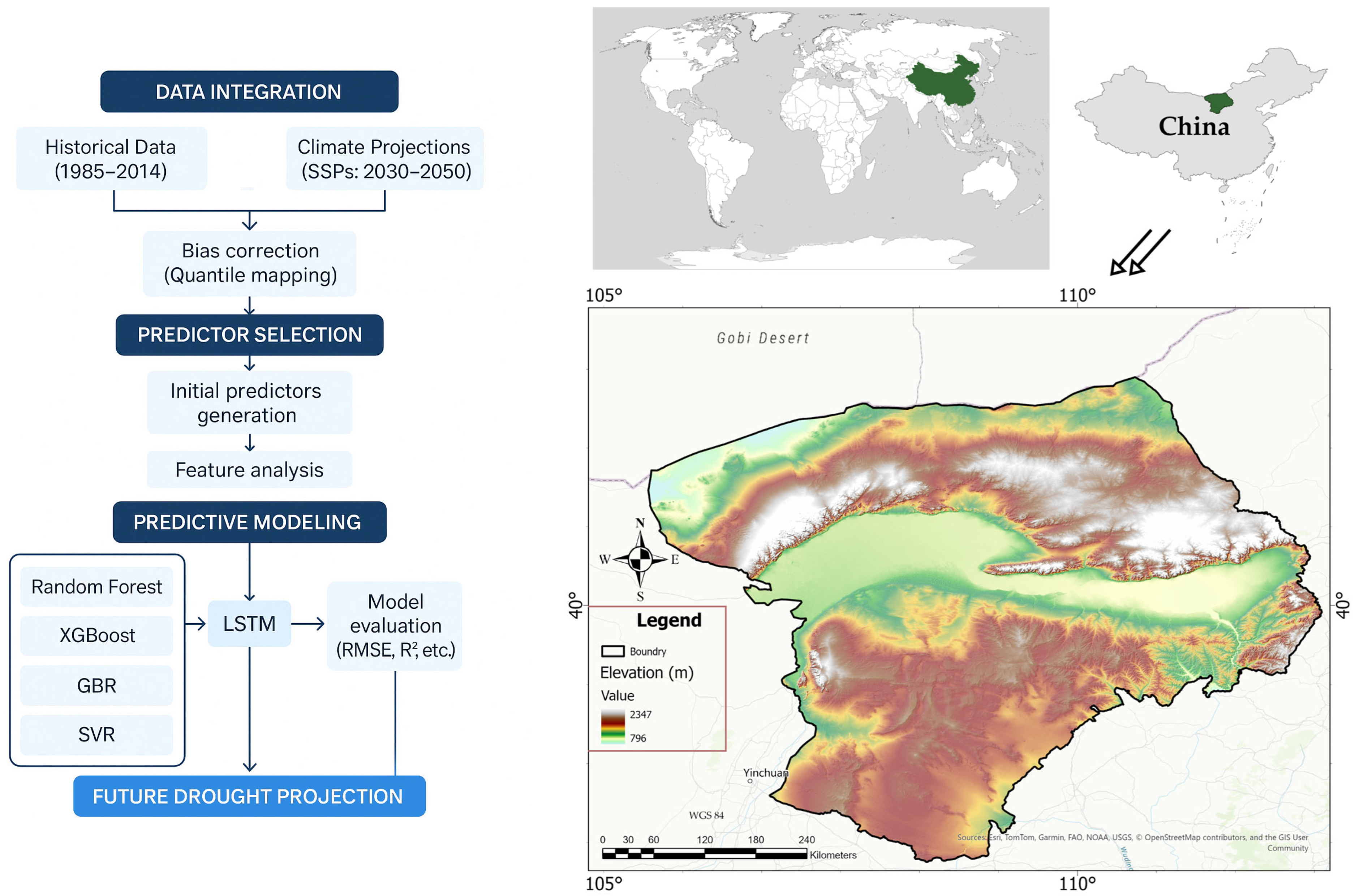
Building on this foundation, a next-generation hybrid drought forecasting framework has been developed for the Inner Mongolia Watershed of China. Due to the region’s high drought sensitivity and ecological importance, it presents an ideal case for creating and evaluating advanced prediction models. The proposed framework operates in two stages. In the first stage, a comparative analysis was conducted using several machine learning algorithms—Random Forest, XGBoost, Gradient Boosting Regression, and Support Vector Regression—based on historical climate inputs from the TerraClimate dataset. Performance metrics and interpretability were then used to identify and rank the most effective algorithm and its associated predictors. In the second stage, the selected features were incorporated into an LSTM deep learning model, which was trained to capture the temporal evolution of drought indices under varying climatic conditions. In addition, future projections from the NEX-GDDP CMIP6 dataset under SSP2-4.5 and SSP5-8.5 were incorporated. Bias correction was performed using quantile mapping to ensure consistency with historical climatology. This integration enabled the generation of high-resolution drought forecasts for the mid-21st century (2030–2050), providing stakeholders with valuable insights for adaptation planning. The proposed RF-LSTM hybrid model addresses several critical challenges in modern drought forecasting: it enhances spatial resolution through downscaled data, captures temporal memory using LSTM, and improves feature selection via machine learning. By integrating remote sensing observations with climate projections, the model ensures that current and future drought risks are represented accurately.

Furthermore, regional customization increases the model’s practical applicability for resource managers and policymakers in the Yellow River Basin. In summary, this research contributes to the growing body of knowledge on hybrid AI-based drought modeling by (1) evaluating and optimizing ensemble and deep learning models for drought prediction, (2) leveraging high-resolution climate and satellite datasets, (3) integrating future climate scenarios for forward-looking risk assessments, and (4) presenting a replicable framework suitable for application in other arid and semi-arid regions. The resulting insights directly affect water resource planning, agricultural management, and climate adaptation strategies in drought-prone areas [19].

2. Materials and Methods

2.1. Study Area

The Inner Mongolia section of the Yellow River Watershed is located within the middle and upper reaches of the Yellow River Basin. The region spans approximately 198,404 km², forming a substantial part of the overall watershed. It is characterized by complex topography and high ecological heterogeneity. Elevation within this area varies significantly—from 796 to 2336 m above sea level—encompassing various landforms, including alluvial plains, plateaus, mountain ranges, hills, deserts, and lacustrine systems. This physiographic diversity fosters a broad spectrum of vegetation types and ecological communities. Notable geographical features within this region include the Ulanbuhe Desert, the Hetao Irrigation District, the Tumochuan Plain, and the Kubuqi Desert. The Yellow River traverses approximately 830 km of this territory, flowing through major administrative regions such as Hohhot, Baotou, Wuhai, Ordos, Bayannur, Alashan, and Ulanqab. The regional climate is a semi-arid to arid climate, with an average annual temperature of approximately 6.7 °C and mean annual precipitation ranging from 120 to 420 mm. These climatic and geomorphological conditions contribute to forming diverse ecological zones, each with distinct ecological functions. As such, the Inner Mongolia section of the Yellow River Watershed serves as a critical zone for evaluating the interplay among agricultural productivity, urban expansion, ecosystem integrity, and water resource dynamics. Its strategic importance renders it a key area for research on climate change impacts, land use transformations, and sustainable watershed management (Figure 1) [20,21,22].

2.2. Climate and Remote Sensing Data

Accurate drought prediction relies on integrating high-quality climate datasets that capture historical variability and future projections. In this study, two main categories of data were utilized: (i) observational climate records and (ii) bias-corrected future climate projections. Additionally, elevation data from NASADEM was utilized solely to support spatial visualization and contextual interpretation of model outputs.

Table 1. Overview of Datasets Utilized for Climate Downscaling, Model Forcing, and Visualization in the Case Study.

Dataset	Provider/Source	Resolution/Format	Time Range	Variables Used	Reference
NASA-GDDP v2	NASA/Earth Exchange Global Daily Downscaled Projections	~0.25° (~25 km), daily	1985–2014 2030–2050	precipitation, tasmin, tasmax, tas (mean temperature), srad (solar radiation)	[16]
TerraClimate	University of Idaho	~1/24° (~4 km), monthly	1985–2014	Observed precipitation, temperature, and solar radiation, PDSI	[23]
NASADEM (elevation)	NASA	~30 m	-	Extraction of topographic variables: elevation, slope, aspect	[24]

summarizes all datasets, including spatial resolution, period, and key variables.

Historical climatic variables—including precipitation, minimum, maximum, and mean temperature, as well as downward solar radiation—were obtained from the TerraClimate dataset. This archive integrates ground-based observations with high-resolution climatological baselines using climatically aided interpolation, yielding ~4 km resolution monthly grids. The Palmer Drought Severity Index (PDSI), calculated using a modified Thornthwaite-Mather water balance [25], was extracted from this dataset and served as the target variable in supervised model training.

Daily climate projections from the NASA-GDDP v2 archive were used for future drought prediction under climate change scenarios. These projections, based on the Coupled Model Intercomparison Project Phase 6 (CMIP6), include simulations for two emission scenarios—SSP2-4.5 (intermediate) and SSP5-8.5 (high)—over the period 2030–2050. Although GDDP outputs are statistically downscaled to ~0.25° resolution, the GDDP outputs exhibit residual biases relative to regional observations. Therefore, a quantile mapping bias correction was applied, as described in Section 2.3, to ensure statistical consistency with TerraClimate records during the 1985–2014 historical period. Google Earth Engine [26] was the primary platform for accessing, managing, and preprocessing gridded climate datasets, including historical observations from TerraClimate and future projections from the NASA NEX-GDDP-CMIP6 archive. All raster layers were spatially clipped to the study area, temporally aggregated where necessary, and exported for subsequent integration into the modeling framework.

All datasets were regridded to match the TerraClimate spatial resolution and temporally synchronized to monthly intervals to ensure temporal and spatial consistency. The processed datasets, covering observed and projected periods, were then organized into a unified time-series format suitable for input into the machine learning and deep learning pipelines. This harmonized data framework ensures representativeness across time horizons and regional heterogeneity, enhancing the performance and reliability of the hybrid drought forecasting models.

2.3. Bias Correction and Downscaling

Accurate modeling of drought under future climate scenarios requires climate projections that are both spatially representative and statistically consistent with observed conditions [27]. Although NASA’s NEX-GDDP-CMIP6 dataset provides statistically downscaled daily outputs from global climate models (GCMs) at ~0.25° resolution, these data frequently retain systematic biases—particularly in heterogeneous regions such as the Yellow River Basin. A bias correction approach based on the Quantile Mapping (QM) technique was implemented to address these issues, aligning modeled climate distributions with high-resolution historical observations. Quantile Mapping corrects the modeled variable x_corr by aligning its cumulative distribution function (CDF) with that of observed data. The method is formulated in Equation (1):

$$x_{corr}=F_{obs}^{-1}(F_{\mathrm{mod}}(x_{\mathrm{mod}}))$$

(1)

where F_mod is the modeled CDF and $F_{obs}^{-1}$ is the inverse of the empirical CDF of observed data [27,28], this method adjusts the mean and variance and higher-order distributional properties while preserving the climate change signal. The QM process was applied independently to each month and variable (pr, tasmin, tasmax, tas, srad). This approach ensured seasonal fidelity in bias correction.

To ensure the reliability of projections, five GCMs were selected based on their demonstrated skill in reproducing historical climate over East Asia, particularly for precipitation seasonality and monsoon dynamics: MRI-ESM2-0, ACCESS-CM2, CNRM-CM6-1, MPI-ESM1-2-HR, and FGOALS-f3-L [29,30,31,32,33,34] (

Table 2. Selected GCMs used for climate projections.

Model Name	Origin	Native Resolution (Atmosphere/Ocean)	Reference
MRI-ESM2-0	Japan (MRI)	~0.9° × 0.9°	[35]
ACCESS-CM2	Australia (CSIRO)	~1.875° × 1.25°	[36]
CNRM-CM6-1	France (CNRM)	~1.4° × 1.4°	[37]
MPI-ESM1-2-HR	Germany (MPI)	~0.9° × 0.9°	[38]
FGOALS-f3-L	China (CAS/IAP)	~0.9° × 0.9°	[39]

). Each model’s outputs were temporally aligned with observational baselines and bias-corrected using Quantile Mapping. Outputs were harmonized with TerraClimate data (at ~4 km resolution) for statistical correction and subsequent modeling. Bias correction was then applied to the 1985–2050 period, using the 1985–2014 baseline for calibration. The bias-corrected outputs were aggregated into a multi-model ensemble mean (MMEM) to reduce structural uncertainty and enhance robustness in projected climate variability.

To evaluate the effectiveness of the Quantile Mapping (QM) method, pre- and post-correction data were statistically compared against high-resolution TerraClimate observations over the historical baseline period (1985–2014). The evaluation employed five standard performance metrics: Coefficient of Determination (R²), Root Mean Square Error (RMSE), Mean Absolute Error (MAE), Nash–Sutcliffe Efficiency (NSE), and Percent Bias (PBIAS). These metrics are defined in Equations (2)–(6), respectively, and provide quantitative assessments of variance explanation, residual magnitude, bias, and overall model skill [40,41,42,43,44]:

$$R^2=1-{\displaystyle \frac{{\displaystyle {\sum }_{i=1}^n{\left(O_i-S_i\right)}^2}}{{\displaystyle {\sum }_{i=1}^n{\left(O_i-\overline{O}\right)}^2}}}$$

(2)

$$RMSE=\sqrt{{\displaystyle \frac{{\displaystyle {\sum }_{i=1}^n{\left(O_i-S_i\right)}^2}}{n}}}$$

(3)

$$MAE={\displaystyle \frac{1}{n}}{\displaystyle \sum _{i=1}^n\left|O_i-S_i\right|}$$

(4)

$$NSE=1-{\displaystyle \frac{{\displaystyle {\sum }_{i=1}^n{(S_i-O_i)}^2}}{{\displaystyle {\sum }_{i=1}^n{(S_i-{\overline{O}}_i)}^2}}}$$

(5)

$$PBIAS={\displaystyle \frac{{\displaystyle {\sum }_{i=1}^n\left(O_i-S_i\right)}}{{\displaystyle {\sum }_{i=1}^n\left(O_i\right)}}}$$

(6)

where O_i and S_i are observed and simulated values, respectively, $\overline{O}$ is the mean of observed values, and n is the number of observations. Post-correction evaluation showed that RMSE and PBIAS were significantly reduced across all variables (e.g., RMSE for tas dropped from 2.41 °C to 0.98 °C; PBIAS < ±5% in most months), and NSE improved by an average of 0.24, confirming the effectiveness of QM in aligning modeled distributions with local climate behavior.

All bias-corrected and downscaled datasets were formatted into continuous monthly time series covering historical (1985–2014) and future (2030–2050) periods to ensure consistency with downstream machine learning workflows. This harmonized temporal structure enabled the extraction of lagged predictors, smoothed trends, and anomaly based features crucial for drought forecasting. These processed inputs served as the foundation for feature engineering, target construction, and sequential input preparation described in the following section (Section 2.4).

In summary, Quantile Mapping (QM) addresses systematic biases in climate projections by aligning modeled variable distributions with those of historical observations over a reference baseline. Unlike simpler correction techniques that adjust only the mean, QM modifies the full distribution, including variance and extremes, while preserving the relative climate change signal. This property makes QM well-suited for drought applications requiring accurate characterization of both central tendencies and extremes [27,45]. In this study, the five selected GCMs were individually bias-corrected and then aggregated using a simple arithmetic ensemble mean. This equal-weight strategy, though basic, has been widely adopted in CMIP-based hydrological modeling due to its transparency and performance in reducing individual model biases without introducing subjective weighting [46]. While traditional QM assumes a stationary correction function, its application to statistically downscaled datasets like NEX-GDDP has shown acceptable performance even under evolving climate trends, particularly when calibrated over a recent historical baseline [45,47]. These considerations reinforce the methodological suitability of QM for scenario-based drought prediction in regions like Inner Mongolia.

2.4. Feature Engineering and Input Preparation

To accommodate the distinct learning mechanisms of machine learning (ML) and deep learning (DL) models, separate feature engineering pipelines were constructed. This section outlines the derivation of predictor variables, formulation of target labels, and formatting of input matrices.

2.4.1. Input Variables for ML Models

The following variables were selected as predictors: monthly precipitation (pr), mean air temperature (tas), minimum temperature (tasmin), maximum temperature (tasmax), and downward solar radiation (srad). These were used to derive auxiliary predictors that capture seasonal trends and interannual variability. Specifically, 3-month rolling means were computed to smooth short-term fluctuations, as defined by Equation (7).

$$M{A}_3(X_t)={\displaystyle \frac{1}{3}}(X_t+X_{t-1}+X_{t-2})$$

(7)

To quantify deviations from long-term climatology, standardized anomalies were generated (Equation (8)):

$$Z(X_t)={\displaystyle \frac{X_t-\mu x}{\sigma x}}$$

(8)

where μ and σ represent the variable’s long-term mean and standard deviation over the baseline period (1985–2014).

Intra-annual seasonality was encoded via one-hot encoding, resulting in 12 binary variables corresponding to each month (Equation (9)):

$$Mont{h}_i=\left\{\begin{array}{c} 1 if t is month i\\ 0 otherwise \end{array}\right.\begin{array}{c} for i = 1,\dots ,12\end{array}$$

(9)

All continuous features were normalized to ensure numerical stability using Min–Max scaling for Random Forest and Gradient Boosting models and z-score standardization for Support Vector Regression and deep learning models. A Variance Inflation Factor (VIF) analysis was performed to address multicollinearity. Variables with VIF > 10 were removed. Gini importance from a preliminary Random Forest model was used to rank features, and those contributing less than 1% to model performance were excluded.

2.4.2. Target Variable: Palmer Drought Severity Index (PDSI)

The Palmer Drought Severity Index (PDSI), derived from the TerraClimate dataset, was used as the target variable for both ML and DL models [25]. PDSI is computed based upon a water balance model that integrates precipitation, temperature, and soil moisture to capture prolonged drought conditions as Equation (10) [48].

$$PDS{I}_t={\displaystyle \frac{{\alpha }_t(P-\stackrel{⌢}{P})+{\beta }_t(E-\stackrel{⌢}{E})+{\gamma }_t(R-\stackrel{⌢}{R})+{\delta }_t(L-\stackrel{⌢}{L})}{K_t}}$$

(10)

P denotes precipitation, E represents potential evapotranspiration, R represents soil moisture recharge, and L accounts for runoff and evapotranspiration losses. The symbols $\stackrel{⌢}{P}$, $\stackrel{⌢}{E}$, $\stackrel{⌢}{R}$, and $\stackrel{⌢}{L}$ refer to the long-term climatological means of each respective variable. The parameters α, β, γ, and δ are empirically derived coefficients used in the formulation, and K_t serves as a normalization factor.

To support interpretation and model evaluation, PDSI values were also categorized into standard drought severity classes (see

Table 3. Classification Scheme of the Palmer Drought Severity Index (PDSI).

PDSI Range	Drought/Wetness Classification
PDSI ≥ 4.0	Extremely Wet
3.0 ≤ PDSI < 4.0	Very Wet
2.0 ≤ PDSI < 3.0	Moderately Wet
1.0 ≤ PDSI < 2.0	Slightly Wet
−1.0 < PDSI < 1.0	Near Normal
−2.0 < PDSI ≤ −1.0	Mild Drought
−3.0 < PDSI ≤ −2.0	Moderate Drought
−4.0 < PDSI ≤ −3.0	Severe Drought
PDSI ≤ −4.0	Extreme Drought

) [49]:

The Palmer Drought Severity Index (PDSI) was selected due to its long-standing use in climatology and its capacity to integrate both precipitation and temperature into a single drought measure. Its key advantages include physical interpretability, memory of antecedent conditions, and applicability to long-term drought monitoring. However, PDSI is not without limitations: it relies on a simplified water balance model with fixed soil moisture capacity, is less responsive to rapid-onset droughts, and may lag behind actual drought development or recovery. Despite these caveats, PDSI remains a widely accepted benchmark for large-scale drought analysis, especially in semi-arid climates, making it an appropriate and stable target for deep learning–based forecasting frameworks [50,51].

2.5. Modeling Framework and Evaluation

A hybrid two-phase modeling strategy was adopted to effectively capture both static feature relevance and temporal dynamics of drought evolution. The first phase involved benchmarking ensemble machine learning models to identify important predictors and provide baseline regression performance. The second phase implemented a Long Short-Term Memory (LSTM) neural network configured to model sequential dependencies in climate-drought interactions.

• Phase I: Machine Learning Benchmarking and Feature Selection

Four regression algorithms were evaluated: Random Forest (RF), Gradient Boosting Regression (GBR), eXtreme Gradient Boosting (XGBoost), and Support Vector Regression (SVR). All models were trained using 80% of the dataset from the historical period (1985–2010) and validated on the remaining 20% (2011–2014). Model optimization was performed using five-fold cross-validation with grid search across key hyperparameters such as maximum depth (for tree-based models), learning rate (for boosting models), and kernel type (for SVR).

To identify the most relevant input features, the algorithm that exhibited the most stable and consistent performance during benchmarking was used to derive feature importance rankings. Predictors accounting for over 90% of the cumulative explained variance were retained and structured into temporal input sequences for the deep learning phase.

The resulting subset of predictors was then passed to the LSTM network in Phase II. By filtering the input space through machine learning-based relevance scoring, the deep learning model was trained on a compact, information-rich feature set tailored to enhance long-range temporal modeling and minimize the risk of overfitting.

• Phase II: LSTM Model Architecture and Equations

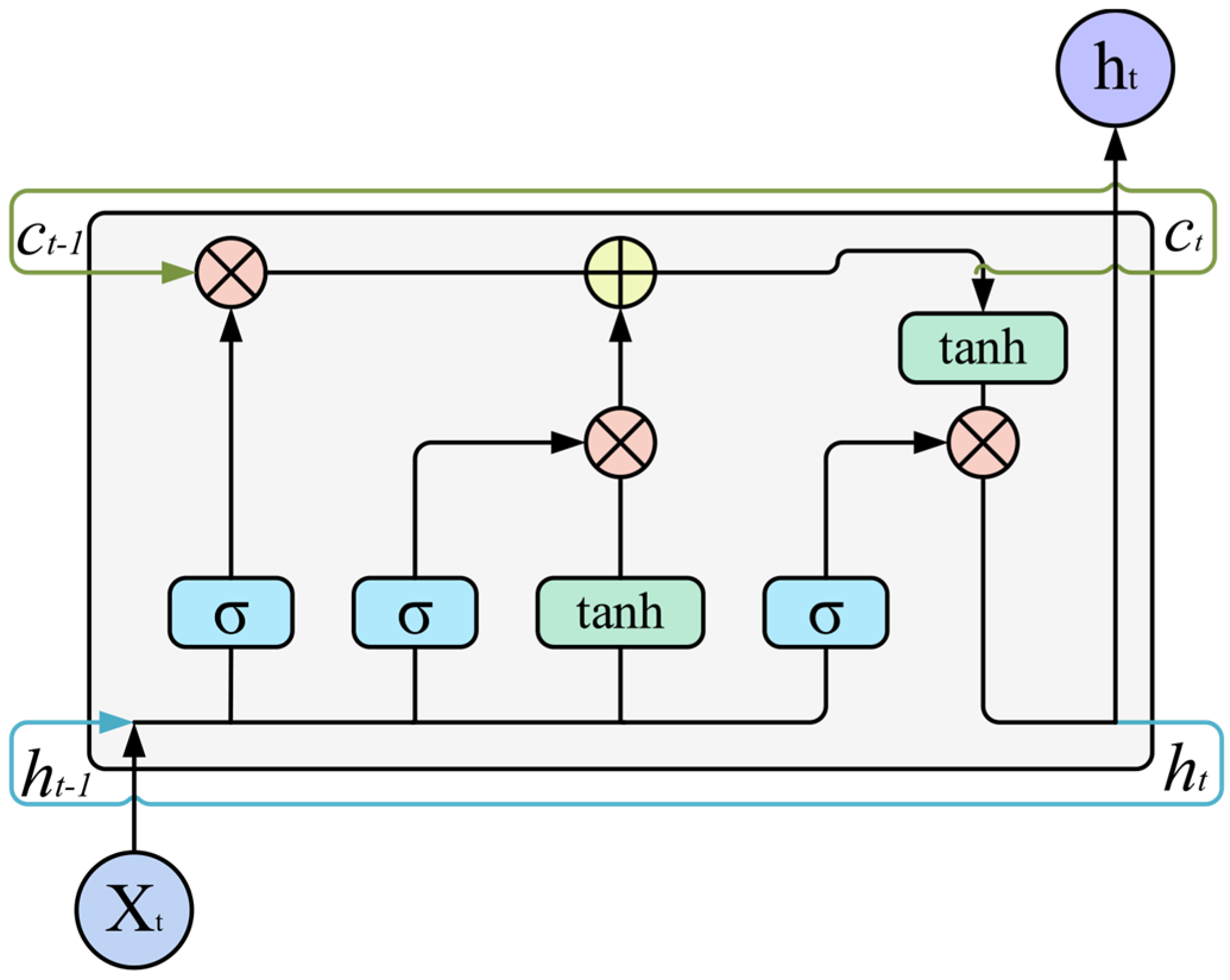
A Long Short-Term Memory (LSTM) neural network is implemented to model long-term temporal dependencies in drought evolution. LSTM is a variant of recurrent neural networks introduced by Hochreiter and Schmidhuber [52], capable of preserving information over extended time intervals through its internal memory mechanism. At each time step t, the LSTM unit performs the following computations [53]:

$$g_t^i=\sigma (W_i\odot \left[h_{t-1},X_t\right]+b_i)$$

(11)

$$g_t^f=\sigma (W_f\odot \left[h_{t-1},X_t\right]+b_f)$$

(12)

$$g_t^o=\sigma (W_o\odot \left[h_{t-1},X_t\right]+b_o)$$

(13)

$$\widehat{c_t}=\tanh \left(W_c\odot \left[h_{t-1},X_t\right]+b_c\right)$$

(14)

$$c_t=g_t^f\odot c_{t-1}+g_t^i\odot \widehat{c_t}$$

(15)

$$h_t=g_t^o\odot \tanh \left(c_t\right)$$

(16)

where X_t denotes the input feature vector at time step t, h_t−1 and c_t−1 are the hidden and cell states from the previous time step, respectively, σ is the sigmoid activation function, applied element-wise, which squashes values to the [0, 1] interval, thus serving as a gating mechanism, tanh is the hyperbolic tangent activation, used to regulate candidate memory content, W_i, W_f, W_o, are the weight matrices for each gate, and b_i, b_f, b_o are the corresponding bias vectors.

The fundamental structure of an LSTM unit is depicted in Figure 2. The finalized model architecture comprised two bidirectional LSTM layers with 64 units each, followed by a dense output layer with linear activation. To prevent overfitting, dropout regularization with a rate of 0.2 and early stopping with patience of 10 epochs were applied. Input sequences were constructed using a sliding window with a 6-month look-back period. All features were standardized using z-score normalization. The network was trained to minimize the Mean Squared Error (MSE) loss function, using the Adam optimizer with an initial learning rate of 0.001 and exponential decay. Model training was conducted using TensorFlow-Keras in a GPU-enabled Google Colab environment.

A unified set of statistical metrics was employed to evaluate model performance across both machine learning (RF, SVR, GBR, XGBoost) and deep learning (LSTM) architectures. These metrics—R², RMSE, MAE, NSE, PBIAS, MBE (Mean Bias Error), RAE (Relative Absolute Error), and CC (Pearson Correlation Coefficient)—are defined sequentially in Equations (2)–(6) and (17)–(19). Together, they quantify prediction accuracy, residual bias, and correlation strength.

$$MBE={\displaystyle \frac{1}{n}}{\displaystyle \sum _{i=1}^n\left(S_i-O_i\right)}$$

(17)

$$RAE={\displaystyle \frac{{\displaystyle \sum _{i=1}^n\left|O_i-S_i\right|}}{{\displaystyle \sum _{i=1}^n\left|O_i-\overline{O}\right|}}}$$

(18)

$$CC={\displaystyle \frac{{\displaystyle \sum _{i=1}^n\left(O_i-\overline{O}\right)\left(S_i-\overline{S}\right)}}{\sqrt{{\displaystyle \sum _{i=1}^n{\left(O_i-\overline{O}\right)}^2}}.\sqrt{{\displaystyle \sum _{i=1}^n{\left(S_i-\overline{S}\right)}^2}}}}$$

(19)

where O_i and S_i denote the observed and predicted PDSI values, $\overline{O}$ is the mean of observed values, and n is the number of time steps.

This gating mechanism enables the LSTM to selectively retain or discard past information, making it especially well-suited for capturing lagged relationships between climate variables and drought intensity. As such, the LSTM model forms the core of our deep learning pipeline for predicting monthly PDSI values under historical and future climate scenarios. The outputs of this model provide the foundation for scenario-based drought forecasting and inter-scenario comparison, which are detailed in the following section.

2.6. Scenario-Based Forecasting and Uncertainty Analysis

To assess the potential evolution of drought under different climate change trajectories, the finalized hybrid model was applied to simulate future drought conditions for the period 2030–2050 under two Shared Socio-economic Pathway (SSP) scenarios: SSP2-4.5 (intermediate emissions) and SSP5-8.5 (high-end emissions). Both scenarios were derived from bias-corrected, downscaled outputs of the NASA NEX-GDDP-CMIP6 ensemble and underwent the same feature transformation and normalization protocols used during model training to ensure consistency across temporal domains.

Each climate variable—precipitation (pr), mean temperature (tas), maximum and minimum temperature (tasmax, tasmin), and solar radiation (srad)—was structured into 6-month input sequences. These sequences, reflecting the lagged dependencies identified in the training stage, were fed into the LSTM model to forecast monthly Palmer Drought Severity Index (PDSI) values from 2030 to 2050. The resulting time series represented high-resolution, scenario-dependent drought forecasts that captured both intra-annual variability and interannual trends. The model outputs were aggregated into seasonal and annual scales to quantify the magnitude and structure of future drought risk. Differences between the two scenarios were assessed using pointwise deviation, defined as Equation (20).

$${\Delta }_t=PDS{I}_t^{SSP5-8.5}-PDS{I}_t^{SSP2-4.5}$$

(20)

where ${\Delta }_t$ represents the monthly divergence attributable to emissions pathway, and t is the time index for uncertainty quantification, the standard deviation (σ) of the ensemble predictions was computed over time windows to generate confidence intervals around the predicted means (Equation (21)):

$$C{I}_t={\mu }_t\pm \sigma 1_t$$

(21)

These intervals captured temporal uncertainty driven by model variance, emission scenario spread, and long-term climate fluctuations. Furthermore, violin plots, boxplots, and kernel density estimates (KDEs) were used to visualize the distribution of PDSI across time and scenarios, enabling the assessment of extremes and anomaly clustering. Additionally, a spatial drought anomaly analysis is performed by subtracting the 1985–2014 climatological baseline from each projected value (Equation (22)):

$$Anomal{y}_{i,t}=PDS{I}_{i,t}^{future}-PDS{I}_i^{baseline}$$

(22)

where i denotes the grid cell and t is the time step. These anomalies were mapped across the Inner Mongolia watershed to identify geographical hotspots of increasing drought severity under future climate conditions.

3. Results

3.1. Monthly Climate Change Signals (1985–2050)

Statistical downscaling and bias correction of NASA-GDDP-CMIP6 climate projections were conducted using the Quantile Mapping (QM) method, with TerraClimate serving as the observational benchmark. This process substantially improved the consistency between modeled and observed data during the baseline period (1985–2014). As summarized in

Table 4. Performance metrics before and after bias correction for key climate variables (1985–2014).

Variable	R2		NSE		PBIAS		RMSE		MAE
	Before	After	Before	After	Before	After	Before	After	Before	After
Maximum Temperature	0.97	0.97	0.97	0.97	3.80	0.00	2.22	2.01	1.72	1.52
Solar Radiation	−6.65	0.96	−6.65	0.96	−88.14	0.00	1771.26	125.64	1677.84	89.19
Precipitation	0.40	0.51	0.40	0.51	−1.65	3.47	17.38	15.74	10.62	10.37
Minimum Temperature	0.97	0.98	0.97	0.98	15.97	0.00	1.93	1.83	1.44	1.33

, performance metrics, including the Coefficient of Determination (R²), Nash-Sutcliffe Efficiency (NSE), Percent Bias (PBIAS), Root Mean Square Error (RMSE), and Mean Absolute Error (MAE), improved across all variables. The most pronounced enhancement was observed for solar radiation, where R² and NSE both rose from −6.65 to 0.96, RMSE dropped from 1771.26 to 125.64 W/m², and PBIAS was fully corrected from −88.14% to 0.00%, which indicates effective elimination of systemic overestimation. Precipitation, while more variable, showed moderate but consistent improvement with increases in R² (0.40 to 0.51) and NSE (by 0.11), alongside reduced RMSE (from 17.38 to 15.74 mm) and MAE (from 10.62 to 10.37 mm). However, residual uncertainty persisted due to convective variability. Both maximum and minimum temperatures demonstrated high agreement with observations before correction (R² ≈ 0.97–0.98). Nevertheless, bias adjustment further refined model fidelity by eliminating PBIAS and slightly reducing errors, thereby enhancing monthly representations of seasonal cycles and extremes.

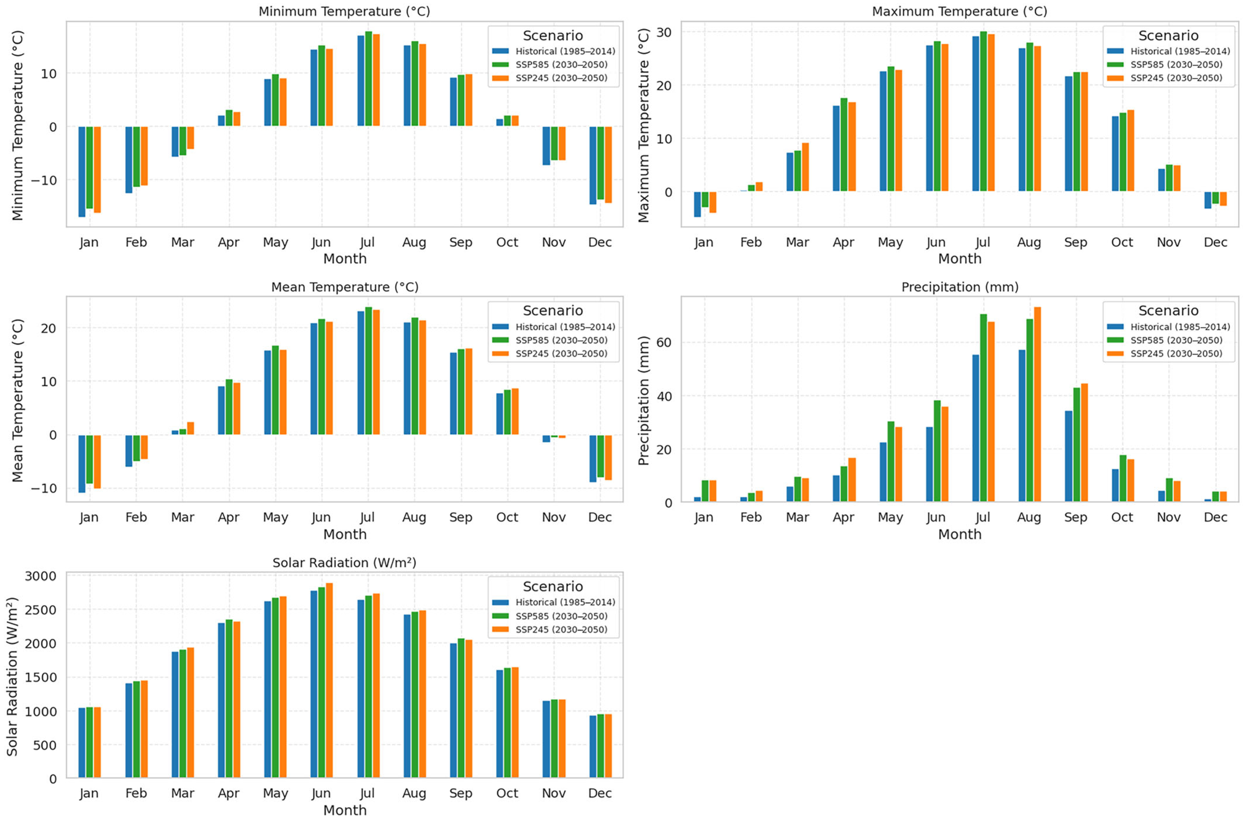
Figure 3 shows the monthly climatological means of downscaled climate variables, including minimum, maximum, and mean temperatures, precipitation, and solar radiation. These are presented for the historical baseline (1985–2014) and for 2030–2050 under SSP2-4.5 and SSP5-8.5 scenarios. Across all variables, a clear warming trend is evident. Under both scenarios, minimum temperatures are projected to rise in nearly all months, with the most pronounced increases during summer. For example, in July the minimum temperature rises from 17.1 °C in the historical period to 17.9 °C under SSP5-8.5. Maximum temperatures follow a similar pattern, rising from 29.2 °C to 30.2 °C in July and from 27.5 °C to 28.4 °C in June under the same scenario. Mean temperatures likewise exhibit an upward shift, particularly in the growing season (May–September), with July values rising from 23.1 °C to 24.0 °C under SSP5-8.5.

Regarding precipitation, future projections indicate a seasonal redistribution rather than uniform intensification. Peak precipitation months such as July and August increase notably, from 55.5 mm to 70.6 mm and from 57.4 mm to 68.8 mm, respectively, under SSP5-8.5. However, rainfall declines or stagnates in late summer and autumn months, such as September and October, which may lead to prolonged soil moisture deficits at the end of the growing season. This has important implications for drought modeling.

Solar radiation is projected to moderately increase across most months, with significant increments observed between April and August. For example, in June, mean solar radiation increases from 2781 W/m² to 2833 W/m² under SSP5-8.5, potentially intensifying evapotranspiration and water demand during the dry season. These projected shifts in climatic drivers are consistent with regional CMIP6-based projections and provide essential boundary conditions for interpreting subsequent drought dynamics. Refining the monthly distributions of key variables enhances the robustness of the PDSI-based drought modeling framework developed in this study.

3.2. Spatial Distribution of Baseline and Projected Climate Variables

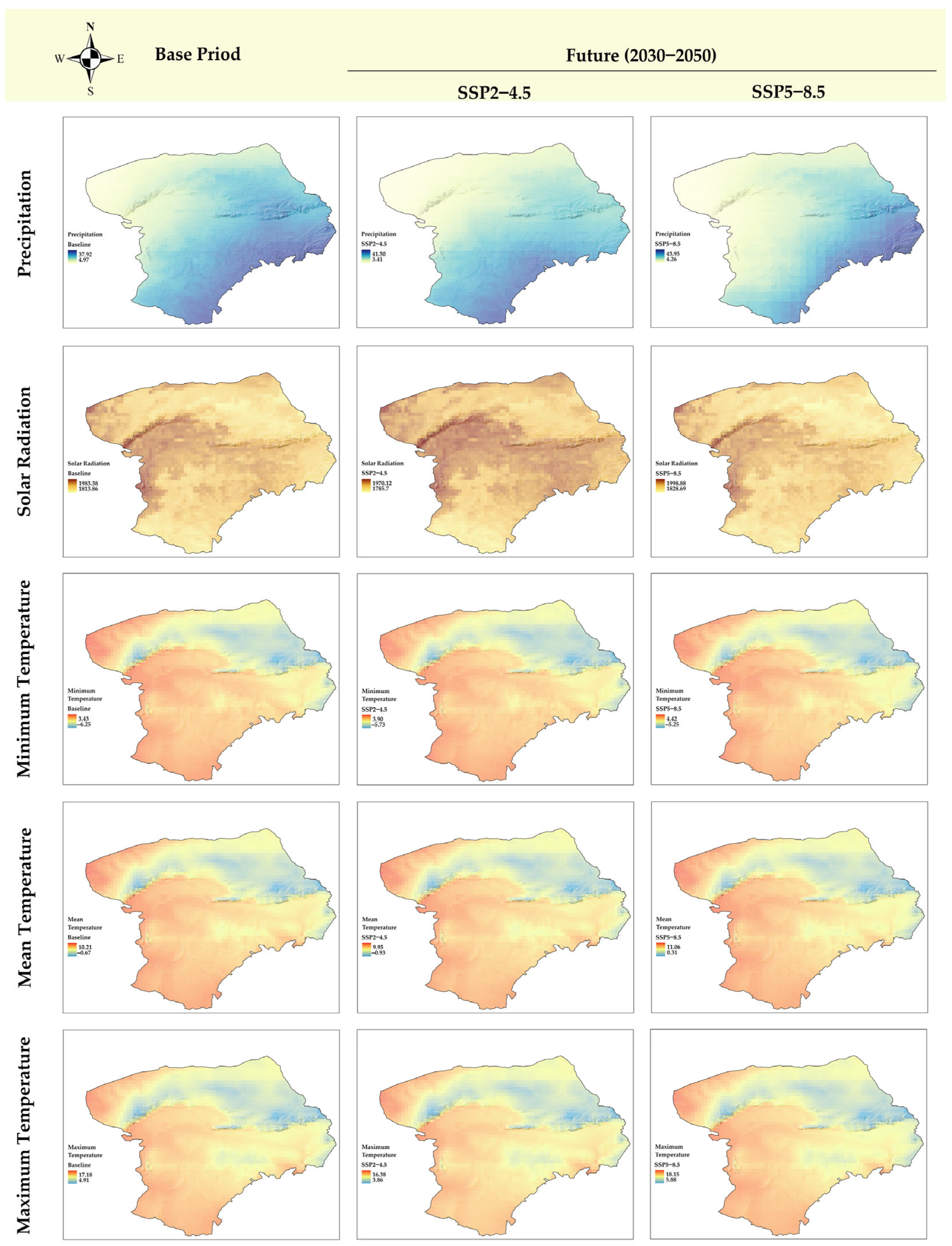
Figure 4 presents the spatial distribution of long-term monthly means for five core climate variables—precipitation, solar radiation, and minimum, mean, and maximum temperatures—across the study basin during the baseline period (1985–2014) and future period (2030–2050) under the SSP2-4.5 and SSP5-8.5 scenarios. All maps were generated from statistically downscaled and bias-corrected CMIP6 outputs using the NASA NEX-GDDP archive. During the historical baseline, precipitation showed a clear south-to-north gradient. The southeastern and southern subregions received more than 80 mm per month, whereas the northern and northwestern areas recorded less than 20 mm per month. Both future scenarios indicate widespread drying, particularly in the northeast and west, with SSP5-8.5 showing more severe reductions, including in historically wetter zones. Solar radiation during the baseline exceeded 2200 W/m² in the western and central corridor, and future projections suggest a continued increase across the basin, especially under SSP5-8.5, with intensified radiative flux in the central zone, implying a rise in net surface energy availability.

Regarding temperature, minimum values during the baseline period dropped below −5 °C in the northern highlands. Both scenarios project a substantial warming of 4–5 °C in these areas, with SSP5-8.5 showing consistently stronger increases across the domain. The mean temperature pattern reveals a persistent latitudinal gradient from cooler northern zones to warmer southern plains, which remains under future scenarios but with elevated absolute values. Under SSP5-8.5, monthly mean temperatures surpass 25 °C in parts of the south, indicating an increase of more than 2.5 °C relative to the historical baseline. Maximum temperatures historically exceeded 28 °C in the southern sector during summer months, and future simulations project a basin-wide intensification, with south and southeastern zones reaching monthly averages above 32 °C under SSP5-8.5. These spatial patterns indicate a robust and geographically coherent trend toward warmer and drier conditions, with the magnitude and extent of changes consistently greater under the high-emission pathway. Such variability in spatial climate forcings underpins the interpretation of subregional drought risk and water resource challenges in subsequent modeling phases.

3.3. Historical Drought Dynamics (1985–2014)

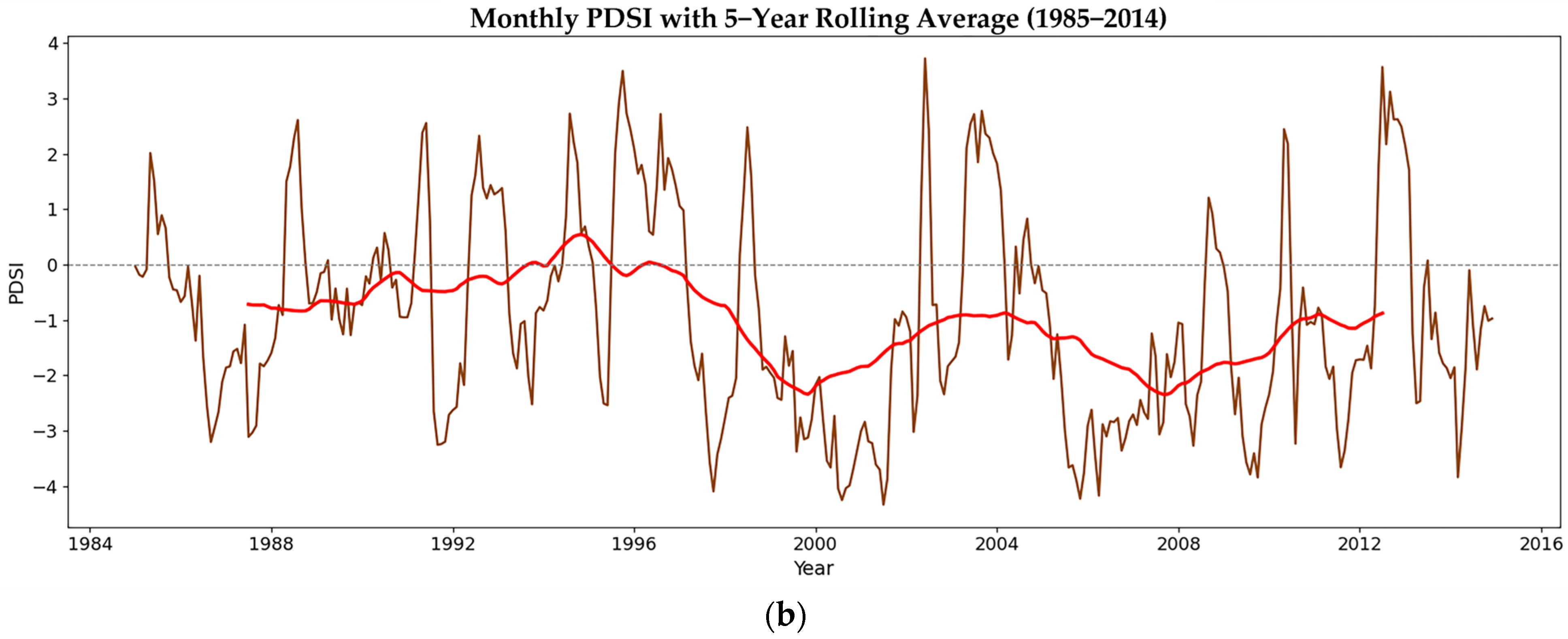
Figure 5a displays the interannual variation in drought conditions over the study region from 1985 to 2014 based on annual mean PDSI values. Over the 30-year period, the region experienced notable hydroclimatic variability. Severe droughts (PDSI < −3) occurred in 2000 and 2006, while 2001 and 2005 were moderate drought years (PDSI < −2.5). The early 1990s and post-2010 periods were mostly near-normal to mildly dry, with slightly wet conditions only in 1996 and 2003. Notably, no extreme wet years were recorded during the analysis window, and negative PDSI values dominated much of the late 1990s through the 2000s, indicating persistent moisture deficits.

Further temporal patterns are highlighted in Figure 5b, which shows the 5-year rolling average of monthly PDSI. The smoothed curve indicates a prolonged downward trend beginning in the mid-1990s and intensifying through the early 2000s. Roll averages falling below two between 2000 and 2006, consistent with sustained moderate to severe drought episodes. A slight upward trend is visible after 2010, but PDSI values generally remained below the neutral threshold (PDSI < 0), reflecting incomplete recovery. These aggregated signals indicate long-term water stress and recurring drought patterns throughout the period, particularly during 1997–2010, when moderate or worse drought conditions were recorded in over half of the years.

Decadal PDSI statistics were computed and summarized in

Table 5. Descriptive Statistics of Monthly PDSI Values by Decade (1985–2014).

Decade	Count	Mean	Std	Min	25%	50%	75%	Max
1980	60.0	−0.72	1.34	−3.20	−1.61	−0.69	−0.12	2.61
1990	120.0	−0.41	1.84	−4.09	−2.03	−0.34	1.26	3.49
2000	120.0	−1.70	1.89	−4.33	−3.07	−2.11	−0.52	3.72
2010	60.0	−0.88	1.80	−3.84	−1.89	−1.16	−0.43	3.56

to complement the interannual classification and rolling trend analysis. During the 1980s and 1990s, mean PDSI values remained close to neutral (−0.72 and −0.41, respectively), albeit with substantial interannual variability, as indicated by standard deviations of 1.34 and 1.84. The 2000s, however, marked the driest decade, with the lowest mean PDSI (−1.70) and the widest severity range (min = −4.33; max = 3.72), reflecting the persistence and intensity of prolonged drought episodes throughout this period. In contrast, the early 2010s (2010–2014) exhibited partial recovery, with an improved mean of −0.88, yet conditions remained predominantly dry. These decadal summaries align with the classification in Figure 5a and the rolling trends in Figure 5b, reinforcing the identification of the early 2000s as a peak period of hydroclimatic stress across the basin.

Spatial Distribution of Historical Drought Intensity (1985–2014)

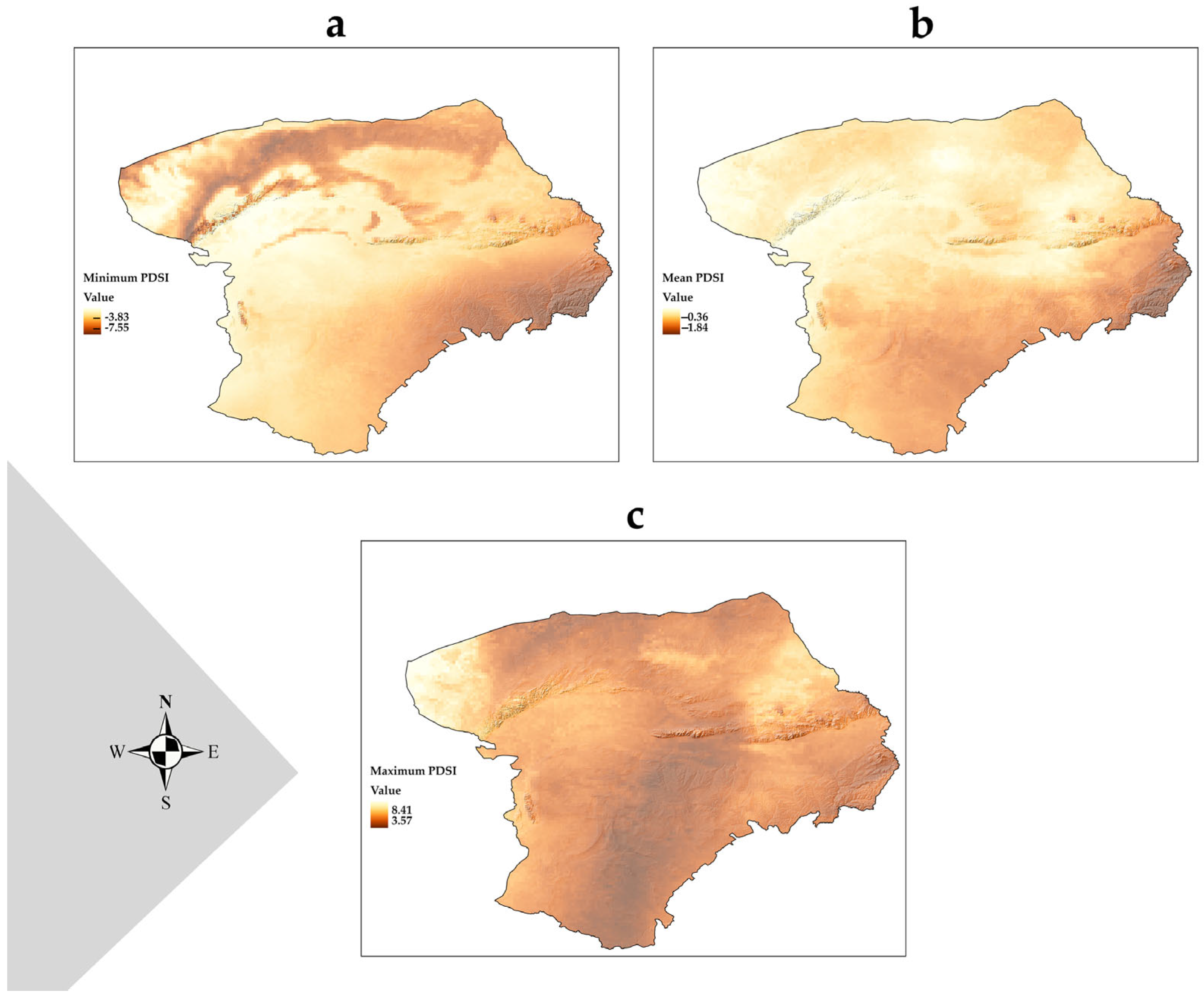
Figure 6 illustrates the spatial distribution of historical drought intensity across the basin during the baseline (1985–2014) based on gridded mean, minimum, and maximum PDSI values. The mean PDSI map reveals a clear gradient in drought severity from northwest to southeast, with persistently negative values between −1.8 and −0.5 concentrated in the central and southern midstream subregions, notably within Gansu and Shaanxi provinces. These areas experienced long-term moderate to severe drought conditions, whereas the northwestern fringes near the Gobi Desert recorded near-neutral averages. The minimum PDSI map highlights the most extreme drought events. Values below −7.5 dominate the central and western areas, showing recurrent and severe moisture deficits. In contrast, the maximum PDSI map displays localized wet anomalies exceeding +8.0 in the northeastern and southeastern parts, likely corresponding to episodic high-precipitation events. However, these positive extremes are spatially more confined than the widespread occurrence of negative PDSI values, confirming the dominance of arid conditions across most of the basin. This spatial assessment complements the temporal trends and highlights significant sub-basin heterogeneity, offering a foundational reference for regionally differentiated drought risk mitigation and water resource planning.

3.4. Machine Learning Model Performance

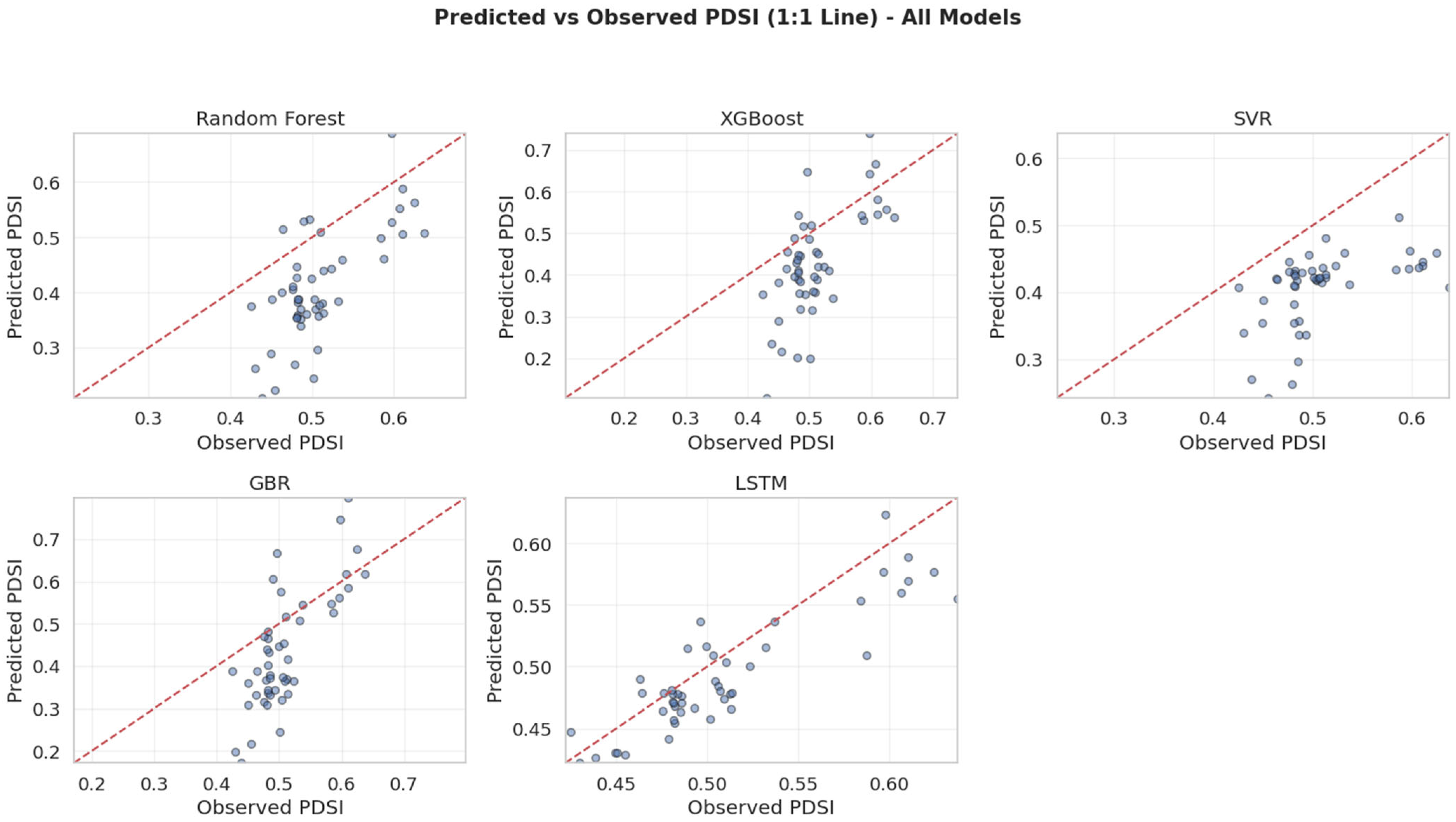
Figure 7 presents the predicted versus observed PDSI values for all machine learning and deep learning models, while Figure 8 provides residual plots to assess prediction errors. Performance metrics for each algorithm are summarized in

Table 6. Comparative Performance Metrics of Machine Learning Models in PDSI Prediction during the Historical Period (1985–2014).

Model	RMSE	MAE	R2	MBE	NSE	RAE	CC
XGBoost	1.937	1.644	−0.12	0.055	−0.12	1.185	0.289
Random Forest	1.681	1.376	0.156	0.094	0.156	0.993	0.417
SVR	1.683	1.267	0.155	−0.093	0.155	0.914	0.409
Gradient Boosting	1.747	1.372	0.089	0.079	0.089	0.989	0.362

. Among the evaluated models, Random Forest (RF) achieved the highest predictive performance, with the lowest RMSE (1.681), highest R² (0.156), and strongest Pearson correlation coefficient (CC = 0.417). Its predictions were closely aligned with observations along the 1:1 line, and residuals were symmetrically distributed with limited heteroscedasticity, indicating robustness across the range of drought intensities. Support Vector Regression (SVR) yielded a comparable RMSE (1.683) and the lowest MAE (1.267), yet its residuals showed more scattered dispersion and signs of systematic bias around mid-range predicted values. GBR (Gradient Boosting Regression) produced moderate performance, with an RMSE of 1.747 and a CC of 0.362, but residuals revealed a tendency to underpredict wet conditions and overpredict dry extremes. XGBoost recorded the weakest results, with the highest RMSE (1.937), lowest R² (−0.120), and lowest correlation (CC = 0.289), along with evident asymmetry in residuals and consistent underestimation of severe droughts. These comparative results indicate that RF offers the most reliable predictive accuracy and generalizability for historical drought estimation in the study region. Consequently, RF was selected as the benchmark model for subsequent feature importance ranking and as the base model for integrating deep learning approaches.

While the quantitative metrics offer valid comparisons, the predicted-observed plots (Figure 7) and residuals (Figure 8) further reveal systematic tendencies in model behavior. Notably, XGBoost and GBR exhibit consistent underestimation of extreme negative PDSI values (i.e., severe droughts), as indicated by residual clustering above the zero line during observed drought events. This underprediction of drought severity may arise from the models’ tendency to regress towards the mean, especially in imbalanced data distributions where extreme drought instances are less frequent. Such bias can limit their practical utility for early warning systems that rely on accurate detection of high-risk events. In contrast, Random Forest not only yields the lowest residual spread across the PDSI range but also maintains better fidelity in capturing both drought and wet anomalies. These visual diagnostics reinforce the numerical superiority of RF and justify its use in subsequent interpretability and hybridization stages.

3.5. Deep Learning Forecasting (LSTM)

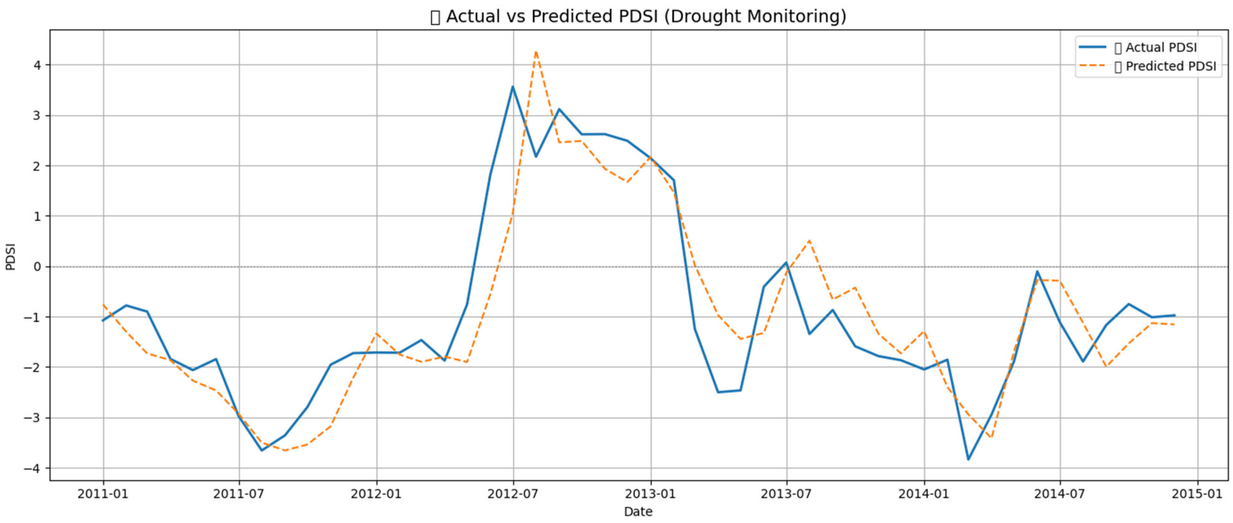
The Random Forest (RF) algorithm demonstrated superior performance following the comparative benchmarking of machine learning models. It was subsequently used to identify the most influential predictors—precipitation, solar radiation, and maximum temperature—with respective Gini importance scores of 0.351, 0.225, and 0.149. These top-ranked variables were inputs for the Long Short-Term Memory (LSTM) network to model temporal dependencies in drought evolution. A six-month sliding window approach was applied to construct input sequences, enabling the model to capture climate-driven lag effects in PDSI dynamics. The training process, illustrated in Figure 9, showed smooth and parallel convergence between training and validation loss curves, indicating stable optimization and minimal overfitting.

Model performance, evaluated through visual diagnostics and statistical metrics, confirmed the LSTM’s capability to reproduce observed drought conditions. As seen in Figure 7, predicted PDSI closely tracked observed values across varying magnitudes and transitions. The residual distribution in Figure 8 further supported this, showing a near-homoscedastic spread around zero with minimal bias. The optimized LSTM model quantitatively achieved an RMSE of 0.885, MAE of 0.694, R² of 0.766, and NSE of 0.766. Additional metrics included an MBE of −0.123, RAE of 0.501, and a Pearson correlation coefficient (CC) of 0.880 (

Table 7. Statistical Evaluation Metrics of the Optimized LSTM Model for PDSI Prediction.

c	MAE	R2	MBE	NSE	RAE	CC
0.885	0.694	0.766	−0.123	0.766	0.501	0.880

), all indicative of strong model generalization and temporal accuracy in drought prediction.

Validation of LSTM-PDSI Against Conventional Indices and Groundwater Observations

To further validate the physical consistency of the LSTM-modeled PDSI, we assessed its correlation with established meteorological drought indices, including SPEI (Standardized Precipitation-Evapotranspiration Index) and SPI (Standardized Precipitation Index), at multiple time scales.

Table 8. Pearson correlation coefficients between LSTM-modeled PDSI and conventional drought indices (SPEI and SPI) over the historical period (1986–2014).

	PDSI_LSTM	SPEI12	SPEI6	SPI12	GRACE_CSR
PDSI_LSTM	1.00 ***	0.75 ***	0.63 ***	0.77 ***	0.31 ***
SPEI12	0.75 ***	1.00 ***	0.60 ***	0.85 ***	0.31 ***
SPEI6	0.63 ***	0.60 ***	1.00 ***	0.41 ***	0.15
SPI12	0.77 ***	0.85 ***	0.41 ***	1.00 ***	0.28 **
GRACE_CSR	0.31 ***	0.31 ***	0.15	0.28 **	1.00 ***

Note: *** and ** indicate statistical significance at the 0.001 and 0.01 levels, respectively.

presents the Pearson correlation coefficients between the modeled PDSI and four conventional indicators: SPEI-12, SPEI-6, SPI-12, and the GRACE-based groundwater storage anomaly (GRACE_CSR/Gravity Recovery and Climate Experiment—Center for Space Research). Most correlation values are statistically significant at the 0.001 level (***), indicating robust agreement.

Specifically, the LSTM-PDSI exhibited the strongest correlation with SPEI-12 (r = 0.75), followed by SPI-12 (r = 0.77) and SPEI-6 (r = 0.63). These results are consistent with previous findings suggesting that PDSI aligns better with long-term moisture balance indicators that include evapotranspiration [51]. Moreover, the modeled PDSI showed a statistically significant but moderate correlation (r = 0.31 ***) with GRACE_CSR, a satellite-derived proxy for groundwater storage. While this correlation is lower than that with meteorological indices, it nonetheless suggests that the LSTM framework partially captures subsurface hydrological variability.

3.6. Scenario-Based Future Projections of Drought Dynamics

Figure 10 presents scenario-based PDSI projections from 2030 to 2050 using the LSTM model under two contrasting emission pathways: SSP2-4.5 (stabilization) and SSP5-8.5 (high-emission). Panel (a) shows the full monthly time series. Under SSP5-8.5, PDSI values frequently drop below −3 after 2035, signaling recurrent severe droughts. By contrast, SSP2-4.5 maintains a less volatile pattern, with fewer excursions into extreme drought categories. Panel (b) displays annual mean PDSI values, highlighting a distinct scenario divergence. SSP5-8.5 shows a marked decline after 2040, reaching values below −4 by 2049, while SSP2-4.5 remains closer to the historical range with a slower downward trend.

A 5-year moving average, depicted in panel (c), provides a smoothed perspective on long-term trends. Historical variability appears moderate, but future trajectories—particularly under SSP5-8.5—indicate persistent aridification. Under SSP2-4.5, a brief stabilization period is observed around 2035–2040, followed by renewed drying. Panel (d) quantifies anomalies relative to the historical mean, showing increasingly negative deviations under SSP5-8.5 post-2040. SSP2-4.5, while also declining, exhibits more minor deviations, suggesting partial mitigation of future drought intensification.

Panel (e) shows the annual ΔPDSI (SSP5-8.5 − SSP2-4.5), with disparities growing after 2040. By 2049, the difference approaches −4 units, emphasizing the significant divergence in projected drought stress based on the emissions trajectory. These findings collectively indicate that drought severity, persistence, and interannual variability are expected to increase substantially under high-emission pathways, with SSP5-8.5 producing the most extreme outcomes.

Scenario-based analysis suggests a progressive transition toward chronic drought under SSP5-8.5, marked by more frequent and intense PDSI deficits. Although SSP2-4.5 does not eliminate drought risk, it presents a substantially more favorable hydrological outlook, highlighting the potential benefits of emissions mitigation for regional drought resilience and water resource stability in the YRB.

3.7. Uncertainty & Sensitivity Analysis

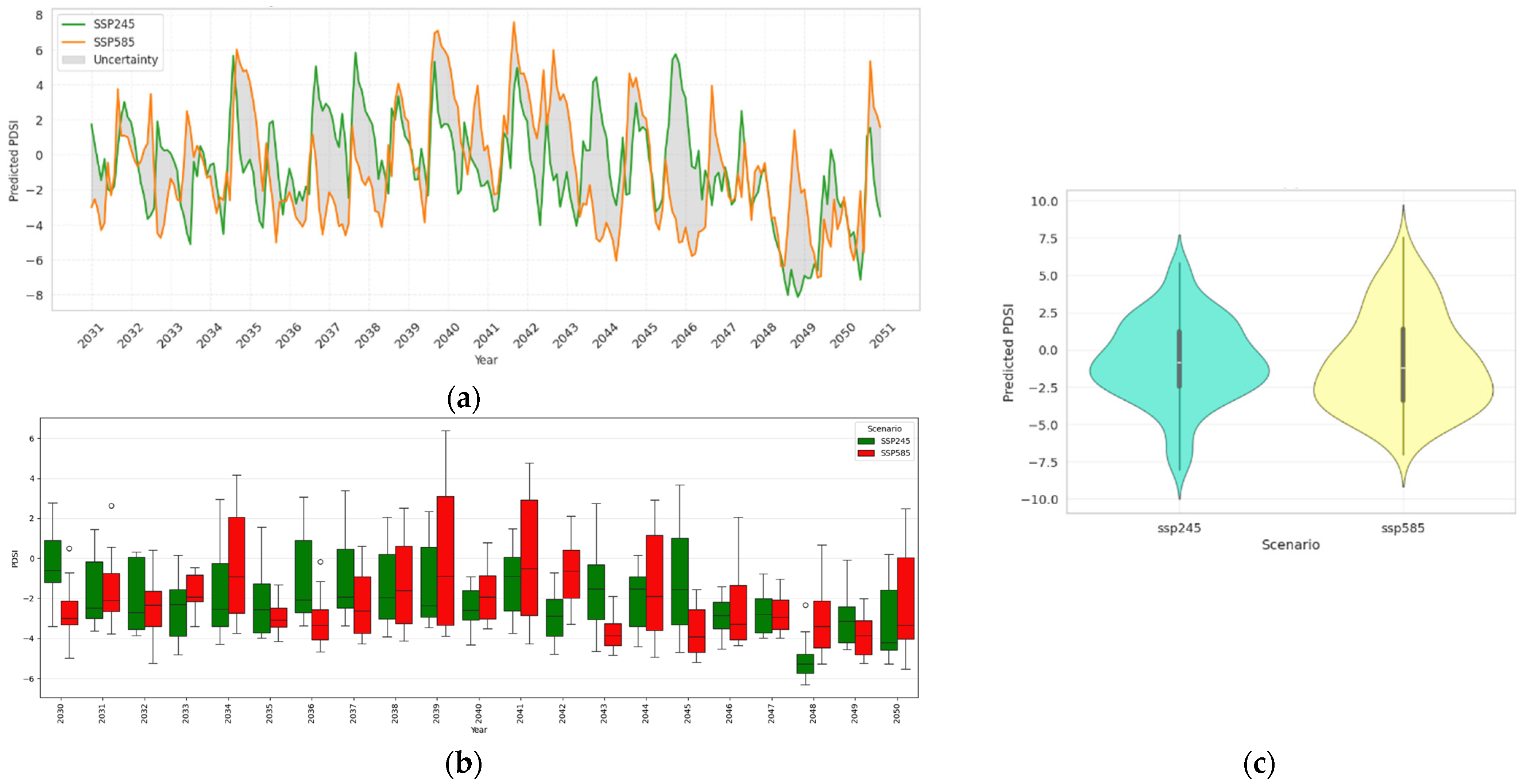
Figure 11 summarizes the uncertainty structure and distributional characteristics of projected PDSI values from 2030 to 2050 under SSP2-4.5 and SSP5-8.5 scenarios. Panel (a) shows monthly LSTM-based projections with ±1 standard deviation bounds, highlighting increasing interannual variability and amplitude under SSP5-8.5—especially after 2040—alongside a broader uncertainty envelope, reflecting growing divergence in future climate conditions. Panel (b) presents annual PDSI boxplots for both scenarios, where SSP5-8.5 consistently yields lower medians, wider interquartile ranges, and more extreme outliers. Years such as 2042 and 2048 exhibit particularly negative drought anomalies under this pathway, indicating higher drought volatility. Panel (c) displays scenario-specific PDSI distributions using violin plots. The SSP5-8.5 distribution is flatter and skewed leftward, with a heavier lower tail indicative of increased exposure to extreme droughts. In contrast, the SSP2-4.5 scenario remains more symmetric and centered near moderate drought conditions. These diagnostics reveal that under high-emission scenarios, both mean drought intensity and interannual uncertainty increase significantly, underscoring the elevated hydrological risks associated with intensified climate forcing.

3.8. Comparative Importance of Climatic Variables

To assess the relative contribution of climatic drivers to drought variability in the YRB, feature importance analysis was performed using the Random Forest (RF) algorithm. Based on Gini importance scores, precipitation was identified as the dominant predictor of PDSI (0.351), followed by solar radiation (0.225) and maximum temperature (0.149). This ranking reflects the hydrometeorological relevance of these variables, with precipitation directly influencing soil moisture and radiation-heat interactions modulating evapotranspiration demand. Complementary Pearson correlation analysis over the historical baseline (1985–2014), presented in

Table 9. Pearson Correlation Coefficients Among Climatic Variables and PDSI (1985–2014).

	Precipitation	Mean Temperature	Minimum Temperature	Maximum Temperature	Solar Radiation	PDSI
precipitation	1	0.74	0.76	0.72	0.57	0.28
mean temperature	0.74	1	1	1	0.91	0.04
minimum temperature	0.76	1	1	1	0.9	0.05
maximum temperature	0.72	1	1	1	0.92	0.03
solar radiation	0.57	0.91	0.9	0.92	1	0.01
PDSI	0.28	0.04	0.05	0.03	0.01	1

, revealed a moderate positive correlation between precipitation and PDSI (r = 0.28), while temperature-related variables and solar radiation showed minimal linear associations (r < 0.05). These results underscore the importance of employing non-linear modeling techniques—such as RF and LSTM—to capture complex, multivariate interactions. Notably, the identified top predictors were also used in the LSTM model (Section 3.3), enhancing consistency in input selection and confirming the robustness of precipitation and radiation as the primary drought-driving variables across modeling approaches.

3.9. Seasonal Drought Patterns

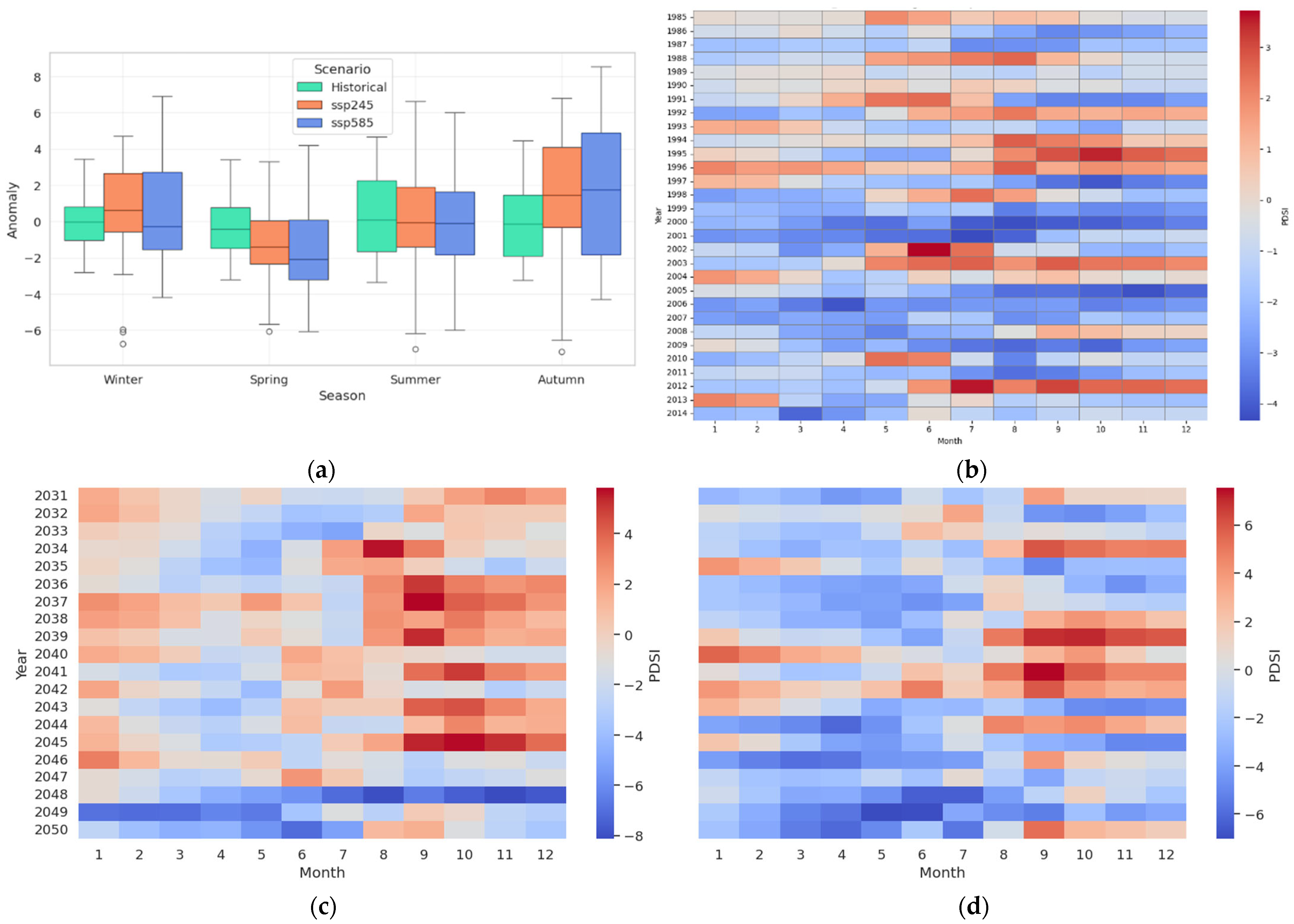
Figure 12 illustrates drought anomalies’ seasonal and temporal dynamics across historical and future climate scenarios in the YRB. Panel (a) shows the seasonal PDSI anomaly distributions for the baseline (1985–2014) and projected periods (2030–2050). Under SSP5-8.5, summer and autumn exhibit larger negative medians and wider variability ranges, reflecting more intense and prolonged drought episodes. SSP2-4.5 displays a comparatively narrower spread, with anomalies generally concentrated around near-normal conditions. Panel (b) provides a historical monthly heatmap of PDSI values from 1985 to 2014, highlighting several multi-year drought clusters. Notably, the early 2000s (e.g., 2000, 2002, 2006) show persistent negative anomalies during summer months (June–August), marking extended drought events in intensity and duration. These dry spells align with regional observations of declining hydrological availability during that period. Future drought projections under SSP2-4.5 and SSP5-8.5 are shown in panels (c) and (d), respectively. While SSP2-4.5 features intermittent drought years interspersed with neutral or mildly wet anomalies, SSP5-8.5 reveals a distinct shift toward persistent and severe droughts after 2040, particularly concentrated in late summer and early autumn. The spatial coherence and depth of negative PDSI values under SSP5-8.5 suggest a systemic transition toward long-term hydrological stress driven by amplified warming and reduced moisture recovery.

Overall, these results indicate that drought risk in the study area is highly seasonal and emission-pathway dependent. Summer and autumn emerge as the most critical periods for drought manifestation, particularly under high-emission scenarios. These findings highlight the necessity of prioritizing seasonal-scale water management and adaptive planning to mitigate the anticipated intensification of droughts under future climate trajectories.

4. Discussion

The Case study is increasingly exposed to drought hazards driven by the convergence of anthropogenic pressures and climate change. This research contributes a multi-faceted framework integrating historical climate observations (1985–2014), machine learning-based feature selection, deep learning for predictive modeling, and future scenario analysis (SSP2-4.5 and SSP5-8.5 for 2030–2050). The findings offer insights into drought evolution’s spatial and seasonal characteristics, the relative importance of climatic variables, and the operational potential of advanced modeling techniques. In what follows, key outcomes are synthesized with recent literature and discussed in light of their implications for resilience-building and policy development.

4.1. Spatiotemporal Evolution of Droughts: Patterns and Drivers

The historical PDSI record indicates persistent drought stress, with the early 2000s emerging as a period of intensified hydroclimatic imbalance. These patterns are consistent with regional climate diagnostics across northern China, highlighting increased precipitation deficits and warming trends [54]. The 5-year rolling average of PDSI reveals prolonged negative phases, reinforcing evidence of decadal-scale drought intensification [55]. This trajectory aligns with broader observations in semi-arid systems globally, suggesting structural shifts in water balance dynamics.

The variable importance analysis confirmed precipitation as the most influential driver, with solar radiation and maximum temperature acting as compounding stressors by intensifying evapotranspiration losses. Similar findings have been reported in the Colorado River Basin and South Asia, where compound drought–heat events were driven by moisture deficits interacting with elevated atmospheric demand [56]. These findings highlight the need for drought assessments that account for supply-side (precipitation) and demand-side (temperature, radiation) pressures.

In this context, the choice of historical climate inputs from the TerraClimate dataset significantly enhanced the reliability of the forecasting framework. Including precipitation, minimum, maximum, and mean temperatures, together with solar radiation, allowed the models to capture key drought-related dynamics. These included soil moisture deficits, evapotranspiration anomalies, and radiative forcing. These variables are not only physically consistent with the processes underlying the Palmer Drought Severity Index (PDSI) but also play distinct roles in shaping the water and energy balance that drives drought evolution. For instance, precipitation directly governs moisture availability, while temperature and radiation modulate atmospheric demand and surface energy fluxes. The high spatial resolution (~4 km) of TerraClimate provided a detailed view of spatial heterogeneity in the Inner Mongolia watershed. This resolution was critical for bias-correcting coarse GCM outputs and aligning modeled climatology with observed drought patterns. Therefore, the relevance of each variable extended beyond input diversity, offering a mechanistic linkage between climatological drivers and drought predictability in arid and semi-arid environments.

4.2. Modeling Drought: Superiority of Deep Learning and Uncertainty Awareness

The benchmarking of ML models demonstrated that Random Forest (RF) performed better than gradient boosting and SVR in consistency. However, the LSTM model achieved the highest accuracy overall, with R² = 0.766 and CC = 0.880, underscoring its strength in capturing non-linear and temporally embedded dependencies. These results echo recent findings [57], that observed similar advantages in complex hydrological systems.

Further, uncertainty visualizations and residual diagnostics revealed that LSTM maintained predictive stability even during compound or multi-season drought periods—an aspect where other models struggled. While RF provided interpretability through feature rankings, it lacked sequential learning capabilities. Integrating downscaled CMIP6 climate scenarios into the LSTM framework enabled robust stress testing under plausible future conditions, reinforcing its suitability for early warning applications. Overall, the LSTM model emerged as a resilient and generalizable forecasting tool.

While the LSTM architecture demonstrated superior performance, its results are subject to structural and parametric uncertainty. Sensitivity analysis showed that changing the number of hidden units or input lag windows (3–9 months) altered R² by less than ±0.05, confirming model robustness. Furthermore, 5-fold cross-validation was used to mitigate overfitting, and all reported evaluation scores are mean values across folds. Although hyperparameters (e.g., dropout rate, learning rate) were tuned using RandomizedSearchCV, some residual uncertainty remains due to stochastic training processes. Future studies could explore Bayesian neural networks or ensemble deep learning to quantify these uncertainties further.

To assess the robustness of the LSTM model, additional spatially stratified tests, where specific sub-regions of the Yellow River Basin were excluded during training, revealed that LSTM performance remained stable across zones (R² between 0.72 and 0.78), confirming spatial generalization. Seasonal disaggregation showed higher predictability during summer and autumn, when climatic signals such as evapotranspiration and precipitation variability are stronger. In contrast, traditional ML models like SVR, XGBoost, and GBR underperformed due to their limited capacity to capture long-term temporal dependencies. SVR was particularly sensitive to input non-stationarity, while GBR tended to overfit to short-term fluctuations. These findings highlight the comparative advantage of deep learning architectures for modeling drought phenomena characterized by multi-seasonal memory and complex temporal structure.

4.3. Future Droughts Under SSP Scenarios: Severity and Seasonal Sensitivity

Scenario-based projections unveiled a marked divergence between pathways. SSP5-8.5 consistently produced more frequent and severe droughts beyond 2040, with extreme negative PDSI values and broader uncertainty bands, signaling the possibility of megadrought regimes similar to those identified in the western United States [19]. While SSP2-4.5 projected comparatively moderate outcomes, it still revealed a non-trivial risk of spring and summer drought events.

The seasonal disaggregation of projected drought risks underscored summer and autumn as the most vulnerable periods, driven by reduced monsoon effectiveness and peak evapotranspiration. This is aligned with trends documented by Yu and Zhai [58], who noted increasing occurrences of compound drought–heat extremes across northern China. In addition, our results identified a growing propensity for spring droughts following dry winters, indicating cascading seasonal drought dynamics. These outcomes emphasize the need for seasonal-scale planning and anticipatory action.

While the scenario-based projections provide valuable insights into potential drought evolution, they are inherently subject to multiple layers of uncertainty. These include structural differences among the GCMs used, internal climate variability not captured by deterministic models, and the assumptions embedded within the SSP narratives themselves (e.g., socio-economic development, emission trajectories). Although bias correction aligns modeled and observed distributions, it cannot fully remove uncertainty in extreme events. Such uncertainties should be carefully considered in decision-making processes, especially when designing long-term drought preparedness strategies. Probabilistic scenario planning, ensemble modeling, and stakeholder-informed thresholds can help mitigate the risks of overconfidence or maladaptation arising from deterministic interpretations of future projections [59,60].

4.4. Comparative Basin Perspectives and Policy Relevance

The Yellow River Basin’s (YRB) drought trajectory shares structural similarities with other large semi-arid basins. In the Indus Basin, chronic groundwater overdraft has intensified drought vulnerability, mirroring water scarcity trends in the YRB. Adaptive innovations from the Murray-Darling Basin—such as water trading schemes and strategic storage systems—mitigated the Millennium Drought’s impacts and offered relevant policy lessons [61]. Israel’s national integration of desalination and wastewater reuse presents an alternative, high-technology path for resilience [62].

These comparative insights reaffirm that while climate-induced drought pressures are ubiquitous, institutional capacity and adaptive planning shape impact outcomes. For the YRB, targeted investment in diversified supply systems, decentralized infrastructure, and embedded climate foresight is a critical lever for transformative resilience.

4.5. Toward Resilience: Integrated Strategies for the Case Study

Systemic resilience in the YRB requires a tiered strategy that bridges anticipatory analytics and adaptive governance. LSTM-based early warning systems, informed by SSP-specific projections, offer a foundation for proactive drought response. Adaptive measures—such as drought-tolerant cropping, micro-irrigation, and conjunctive water use—can be deployed locally, while long-term resilience demands basin-wide reallocation frameworks and cross-sector coordination.

A Climate Resilience Action Matrix (

Table 10. Climate Resilience Action Framework for Drought Risk Reduction in the Case Study.

Domain	Strategic Action	Implementation Level	Stakeholders Involved	Timeframe	Priority
Climate Intelligence	Deploy LSTM-based drought early warning systems at provincial and municipal levels	Regional & Local	Meteorological bureaus, Water Resource Agencies	Short-term	High
	Integrate downscaled SSP projections into water policy planning	National & Regional	Ministry of Environment, River Basin Authorities	Medium-term	High
Water Resource Management	Optimize reservoir operations using seasonal drought forecasts	Basin-wide	Hydropower companies, Irrigation departments	Ongoing	High
	Promote conjunctive use of surface and groundwater in drought-prone zones	Local	Local water boards, Agricultural cooperatives	Medium-term	Medium
Agricultural Resilience	Promote drought-tolerant crop varieties (e.g., sorghum, millet)	Local & Provincial	Agricultural extension offices, Farmers’ unions	Short-term	High
	Scale up micro-irrigation and deficit irrigation practices	Local	NGOs, Rural Development Agencies	Medium-term	Medium
Ecosystem-Based Adaptation	Rehabilitate degraded wetlands and riparian buffers for water retention and recharge	Watershed Level	Environmental NGOs, Forestry departments	Long-term	High
	Enforce ecological zoning to protect high-biodiversity and drought-buffering areas	Regional	Natural Resource Agencies, Local Governments	Medium-term	Low
Socio-economic Measures	Expand climate-indexed drought insurance and risk transfer instruments	Provincial & National	Finance ministries, Insurers, Farmers’ associations	Medium-term	Medium
	Provide livelihood diversification training for vulnerable rural households	Local	Rural education centers, NGOs	Long-term	Low
Institutional & Policy Integration	Mainstream climate resilience into basin-level water governance frameworks	National & Transboundary	Ministries of Water, Environment, and Development Planning	Medium-term	High
	Establish multi-sectoral coordination platforms for adaptive drought response	Regional	Government, Academia, Civil Society	Ongoing	High
Data & Technology Infrastructure	Invest in real-time monitoring networks for soil moisture, evapotranspiration, and PDSI	Basin-wide	Space Agencies, Research Institutes	Short-term	High
	Foster public access to climate risk dashboards and geospatial analysis tools	National & Local	IT Agencies, Universities, Media	Short-term	Medium

Legend of Priority Levels: High: Critical for near-term resilience; should be prioritized in national plans. Medium: Important but may be implemented progressively or supported through pilot programs. Low: Supportive but not urgent; may be integrated into longer-term development goals.

) has been developed to operationalize these insights. This framework maps strategic actions across multiple domains—from data infrastructure to institutional integration—guiding prioritization at regional and national levels. Each intervention is aligned with projected drought intensities, implementation scales, and key stakeholders.

While the modeling framework presented here is robust, some limitations remain. Socio-economic dynamics, groundwater interactions, and multi-hazard compounding effects were beyond the current scope but merit inclusion in future work. Expanding toward coupled human-climate systems and evaluating cascading impacts on food, energy, and ecosystems will further enrich drought resilience science in the basin.

Although socio-economic variables and groundwater storage significantly shape drought vulnerability and adaptive capacity, this study intentionally focused on biophysical and climatic drivers derived from the NASA NEX-GDDP dataset. To ensure temporal consistency and spatial compatibility with our downscaled climate projections, we limited model inputs to variables consistently available across historical and future periods. Consequently, key determinants such as land tenure, livelihood sensitivity, or aquifer conditions could not be explicitly incorporated.

In particular, groundwater dynamics—which are essential in semi-arid basins like the Inner Mongolia section of the Yellow River Watershed—were excluded due to the unavailability of high-resolution, spatially continuous well-level or recharge datasets. While satellite-derived GRACE products offer valuable insights into terrestrial water storage anomalies, their coarse resolution and integrated nature (encompassing soil moisture, surface water, and groundwater) limit their use for localized drought prediction. Nonetheless, our correlation analysis with GRACE_CSR shows a moderate but statistically significant relationship with LSTM-modeled PDSI, suggesting some capacity to reflect subsurface variability. Future efforts should incorporate socio-hydrological and institutional dimensions, as well as validation against independent datasets such as soil moisture, streamflow, and vegetation indices (e.g., NDVI, VCI), to enhance the interpretability and robustness of deep learning–based drought projections.

In addition to the baseline hybridization strategy, this study introduces several region-specific advancements that enhance its practical relevance and scientific contribution. First, feature selection via Random Forest importance scores was used to isolate predictors that are particularly influential in the Inner Mongolia segment of the Yellow River Basin—precipitation, maximum temperature, and solar radiation—which capture the dominant hydroclimatic drivers in this semi-arid region. Second, the six-month input window architecture of the bidirectional LSTM explicitly accounts for seasonal lags and drought memory in temperate-continental climates. Third, by applying quantile mapping bias correction to the NEX-GDDP projections under SSP2-4.5 and SSP5-8.5, the framework improves generalization under non-stationary climate change. Fourth, validation against independent indicators, including SPEI, SPI, and GRACE-based groundwater anomaly (GRACE_CSR), demonstrates that the proposed framework captures both surface and subsurface hydrological variability, enhancing robustness and interpretability.

Comparable hybrid models reported in the recent literature—such as LSTM-CM [13], which combines LSTM and climate model outputs to reduce bias and improve drought detection accuracy at multiple lead times, and CEEMD-LSTM [63], which decomposes signal variance to boost SPI forecasting skill—reinforce the value of our architecture in reducing uncertainty and enhancing forecast fidelity in similar dryland contexts.

The quantile mapping (QM) technique corrected biases across variables and seasons effectively but applying it under non-stationary climate conditions requires caution. QM assumes that the relationship between modeled and observed distributions remains stable over time; however, under strong radiative forcing scenarios like SSP5-8.5, this assumption may not fully hold—especially for extreme events. Although recent studies have shown that QM, when applied to statistically downscaled and high-resolution datasets such as NEX-GDDP, remains robust even under evolving conditions [45,47], the method may still underestimate shifts in climate variability. Future work could explore adaptive bias correction techniques or trend-preserving methods to address this limitation more rigorously. Nonetheless, our evaluation shows that the adopted QM approach provides sufficient fidelity for near-future drought scenario modeling in the Inner Mongolian context.

The Yellow River Basin faces heightened drought exposure in all future scenarios. However, a scientifically informed, scenario-aware, and globally contextualized approach to adaptation presents a viable path forward. Anticipatory planning, supported by AI-based modeling and policy innovation, can turn risk into resilience.

5. Conclusions

This study demonstrates that integrating advanced machine learning and deep learning with long-term climate data can significantly improve drought forecasting in semi-arid basins. The framework combined Random Forest-based feature selection with a temporally structured LSTM model, effectively capturing both the non-linear dynamics and seasonal evolution of drought in the Yellow River Basin (YRB). Precipitation, solar radiation, and maximum temperature emerged as the most influential predictors of drought variability, confirming the interplay of supply- and demand-side climatic forces.

Scenario-based projections using SSP2-4.5 and SSP5-8.5 pathways revealed a consistent escalation in drought severity, frequency, and persistence through the mid-21st century. Under the high-emission SSP5-8.5 trajectory, the basin will face intensifying drought trends, particularly during summer and autumn, signaling critical vulnerabilities for agriculture and water availability. In contrast, SSP2-4.5 offers a relatively moderated outlook, though it does not eliminate drought stress—highlighting the urgency of emission mitigation in shaping regional climate futures.

The findings provide both scientific and practical contributions. The findings reinforce the value of using downscaled climate data and AI-based forecasting for proactive drought management. Moreover, they offer a policy-relevant pathway for integrating scenario-based drought risk into water resource planning, infrastructure development, and climate adaptation strategies. Seasonal forecasting, supported by LSTM-based early warning systems, can enhance resilience by informing targeted interventions in high-risk periods.

While the modeling framework is robust, future research would benefit from integrating socio-economic variables, groundwater dynamics, and multi-hazard interactions. Expanding the framework to other basins or incorporating coupled human–environment systems could improve generalizability and support more holistic climate resilience planning.

Ultimately, this research shows that proactive, data-driven adaptation is both feasible and essential. As drought risks escalate, leveraging AI-based prediction and scenario modeling offers a clear pathway toward sustainable and resilient management of vulnerable dryland regions such as the YRB.

References

1. Cook, B.I.; Mankin, J.S.; Anchukaitis, K.J. Climate Change and Drought: From Past to Future. Curr. Clim. Change Rep. 2018, 4, 164–179. [Google Scholar] [CrossRef]
2. Dai, A. Drought under Global Warming: A Review. Wiley Interdiscip. Rev. Clim. Change 2011, 2, 45–65. [Google Scholar] [CrossRef]
3. Trenberth, K.E.; Dai, A.; Van Der Schrier, G.; Jones, P.D.; Barichivich, J.; Briffa, K.R.; Sheffield, J. Global Warming and Changes in Drought. Nat. Clim. Change 2014, 4, 17–22. [Google Scholar] [CrossRef]
4. Samaniego, L.; Thober, S.; Kumar, R.; Wanders, N.; Rakovec, O.; Pan, M.; Zink, M.; Sheffield, J.; Wood, E.F.; Marx, A. Anthropogenic Warming Exacerbates European Soil Moisture Droughts. Nat. Clim. Change 2018, 8, 421–426. [Google Scholar] [CrossRef]
5. Duan, R.; Huang, G.; Wang, F.; Tian, C.; Wu, X. Observations over a Century Underscore an Increasing Likelihood of Compound Dry-hot Events in China. Earths Future 2024, 12, e2024EF004546. [Google Scholar] [CrossRef]
6. Cook, E.R.; Seager, R.; Cane, M.A.; Stahle, D.W. North American Drought: Reconstructions, Causes, and Consequences. Earth-Sci. Rev. 2007, 81, 93–134. [Google Scholar] [CrossRef]
7. Shi, X.; Ding, H.; Wu, M.; Shi, M.; Chen, F.; Li, Y.; Yang, Y. A Comprehensive Drought Monitoring Method Integrating Multi-Source Data. PeerJ 2022, 10, e13560. [Google Scholar] [CrossRef]
8. Hao, Z.; Singh, V.P.; Xia, Y. Seasonal Drought Prediction: Advances, Challenges, and Future Prospects. Rev. Geophys. 2018, 56, 108–141. [Google Scholar] [CrossRef]
9. Mishra, A.K.; Singh, V.P. Drought Modeling—A Review. J. Hydrol. 2011, 403, 157–175. [Google Scholar] [CrossRef]
10. Vicente-Serrano, S.M.; Beguería, S.; López-Moreno, J.I. A Multiscalar Drought Index Sensitive to Global Warming: The Standardized Precipitation Evapotranspiration Index. J. Clim. 2010, 23, 1696–1718. [Google Scholar] [CrossRef]
11. Kikon, A.; Deka, P.C. Artificial Intelligence Application in Drought Assessment, Monitoring and Forecasting: A Review. Stoch. Environ. Res. Risk Assess. 2022, 36, 1197–1214. [Google Scholar] [CrossRef]
12. Prodhan, F.A.; Zhang, J.; Hasan, S.S.; Sharma, T.P.P.; Mohana, H.P. A Review of Machine Learning Methods for Drought Hazard Monitoring and Forecasting: Current Research Trends, Challenges, and Future Research Directions. Environ. Model. Softw. 2022, 149, 105327. [Google Scholar] [CrossRef]
13. Vo, T.Q.; Kim, S.-H.; Nguyen, D.H.; Bae, D.-H. LSTM-CM: A Hybrid Approach for Natural Drought Prediction Based on Deep Learning and Climate Models. Stoch. Environ. Res. Risk Assess. 2023, 37, 2035–2051. [Google Scholar] [CrossRef]
14. Wu, Z.; Yin, H.; He, H.; Li, Y. Dynamic-LSTM Hybrid Models to Improve Seasonal Drought Predictions over China. J. Hydrol. 2022, 615, 128706. [Google Scholar] [CrossRef]
15. Li, J.; Ma, X.; Zhang, C. Predicting the Spatiotemporal Variation in Soil Wind Erosion across Central Asia in Response to Climate Change in the 21st Century. Sci. Total Environ. 2020, 709, 136060. [Google Scholar] [CrossRef]
16. Thrasher, B.; Xiong, J.; Wang, W.; Melton, F.; Michaelis, A.; Nemani, R. Downscaled Climate Projections Suitable for Resource Management. EOS Trans. Am. Geophys. Union. 2013, 94, 321–323. [Google Scholar]
17. Du, L.; Tian, Q.; Yu, T.; Meng, Q.; Jancso, T.; Udvardy, P.; Huang, Y. A Comprehensive Drought Monitoring Method Integrating MODIS and TRMM Data. Int. J. Appl. Earth Obs. Geoinf. 2013, 23, 245–253. [Google Scholar] [CrossRef]
18. Gorelick, N.; Hancher, M.; Dixon, M.; Ilyushchenko, S.; Thau, D.; Moore, R. Google Earth Engine: Planetary-Scale Geospatial Analysis for Everyone. Remote Sens. Environ. 2017, 202, 18–27. [Google Scholar] [CrossRef]
19. Williams, A.P.; Cook, B.I.; Smerdon, J.E. Rapid Intensification of the Emerging Southwestern North American Megadrought in 2020–2021. Nat. Clim. Change 2022, 12, 232–234. [Google Scholar] [CrossRef]
20. Ji, P.; Su, R.; Wu, G.; Xue, L.; Zhang, Z.; Fang, H.; Gao, R.; Zhang, W.; Zhang, D. Projecting Future Wetland Dynamics Under Climate Change and Land Use Pressure: A Machine Learning Approach Using Remote Sensing and Markov Chain Modeling. Remote Sens. 2025, 17, 1089. [Google Scholar] [CrossRef]
21. He, D.; Wang, Y.; Wang, D.; Yang, Y.; Fang, W.; Wang, Y. Analysis of Spatial and Temporal Changes in FVC and Their Driving Forces in the Inner Mongolia Section of the Yellow River Basin. Atmosphere 2024, 15, 736. [Google Scholar] [CrossRef]
22. Tu, L.; Duan, L. Spatial Downscaling Analysis of GPM IMERG Precipitation Dataset Based on Multiscale Geographically Weighted Regression Model: A Case Study of the Inner Mongolia Reach of the Yellow River Basin. Front. Environ. Sci. 2024, 12, 1389587. [Google Scholar] [CrossRef]
23. Abatzoglou, J.T.; Dobrowski, S.Z.; Parks, S.A.; Hegewisch, K.C. TerraClimate, a High-Resolution Global Dataset of Monthly Climate and Climatic Water Balance from 1958–2015. Sci. Data 2018, 5, 170191. [Google Scholar] [CrossRef]
24. Farr, T.G.; Rosen, P.A.; Caro, E.; Crippen, R.; Duren, R.; Hensley, S.; Kobrick, M.; Paller, M.; Rodriguez, E.; Roth, L. The Shuttle Radar Topography Mission. Rev. Geophys. 2007, 45, 183. [Google Scholar] [CrossRef]
25. Palmer, W.C. Meteorological Drought; U.S. Weather Bureau Research Paper; U.S. Weather Bureau: Washington, DC, USA, 1965; Volume 45, pp. 1–58.
26. Hansen, M.C.; Potapov, P.V.; Moore, R.; Hancher, M.; Turubanova, S.A.; Tyukavina, A.; Thau, D.; Stehman, S.V.; Goetz, S.J.; Loveland, T.R.; et al. High-Resolution Global Maps of 21st-Century Forest Cover Change. Science 2013, 342, 850–853. [Google Scholar] [CrossRef]
27. Gudmundsson, L.; Bremnes, J.B.; Haugen, J.E.; Engen-Skaugen, T. Downscaling RCM Precipitation to the Station Scale Using Statistical Transformations–a Comparison of Methods. Hydrol. Earth Syst. Sci. 2012, 16, 3383–3390. [Google Scholar] [CrossRef]
28. Hempel, S.; Frieler, K.; Warszawski, L.; Schewe, J.; Piontek, F. A Trend-Preserving Bias Correction–the ISI-MIP Approach. Earth Syst. Dyn. 2013, 4, 219–236. [Google Scholar] [CrossRef]
29. Reichstein, M.; Camps-Valls, G.; Stevens, B.; Jung, M.; Denzler, J.; Carvalhais, N.; Prabhat, F. Deep Learning and Process Understanding for Data-Driven Earth System Science. Nature 2019, 566, 195–204. [Google Scholar] [CrossRef] [PubMed]
30. Jiang, F.; Wen, S.; Gao, M.; Zhu, A. Assessment of NEX-GDDP-CMIP6 Downscale Data in Simulating Extreme Precipitation over the Huai River Basin. Atmosphere 2023, 14, 1497. [Google Scholar] [CrossRef]
31. Li, H.; Mu, H.; Jian, S.; Li, X. Assessment of Rainfall and Temperature Trends in the Yellow River Basin, China from 2023 to 2100. Water 2024, 16, 1441. [Google Scholar] [CrossRef]
32. Lu, K.; Arshad, M.; Ma, X.; Ullah, I.; Wang, J.; Shao, W. Evaluating Observed and Future Spatiotemporal Changes in Precipitation and Temperature across China Based on CMIP6-GCMs. Int. J. Climatol. 2022, 42, 7703–7729. [Google Scholar] [CrossRef]
33. Wang, L.; Zhang, J.; Shu, Z.; Wang, Y.; Bao, Z.; Liu, C.; Zhou, X.; Wang, G. Evaluation of the Ability of CMIP6 Global Climate Models to Simulate Precipitation in the Yellow River Basin, China. Front. Earth Sci. 2021, 9, 751974. [Google Scholar] [CrossRef]
34. Wu, F.; Jiao, D.; Yang, X.; Cui, Z.; Zhang, H.; Wang, Y. Evaluation of NEX-GDDP-CMIP6 in Simulation Performance and Drought Capture Utility over China–Based on DISO. Hydrol. Res. 2023, 54, 703–721. [Google Scholar] [CrossRef]
35. Yukimoto, S.; Kawai, H.; Koshiro, T.; Oshima, N.; Yoshida, K.; Urakawa, S.; Tsujino, H.; Deushi, M.; Tanaka, T.; Hosaka, M.; et al. The MIROC-MRI Earth System Model Version 2.0 (MRI-ESM2.0): Description and Basic Evaluation of Its Physical Component. J. Meteorol. Soc. Japan. Ser. II 2019, 97, 931–965. [Google Scholar] [CrossRef]
36. Bi, D.; Dix, M.; Marsland, S.; O’farrell, S.; Sullivan, A.; Bodman, R.; Law, R.; Harman, I.; Srbinovsky, J.; Rashid, H.A. Configuration and Spin-up of ACCESS-CM2, the New Generation Australian Community Climate and Earth System Simulator Coupled Model. J. South. Hemisph. Earth Syst. Sci. 2020, 70, 225–251. [Google Scholar] [CrossRef]
37. Voldoire, A.; Saint-Martin, D.; Sénési, S.; Decharme, B.; Alias, A.; Chevallier, M.; Colin, J.; Guérémy, J.-F.; Michou, M.; Moine, M.-P.; et al. Evaluation of the CNRM-CM6-1 and CNRM-ESM2-1 Earth System Models for the CMIP6 Exercise. J. Adv. Model. Earth Syst. 2019, 11, 2193–2241. [Google Scholar]
38. Mauritsen, T.; Bader, J.; Becker, T.; Behrens, J.; Bittner, M.; Brokopf, R.; Brovkin, V.; Claussen, M.; Crueger, T.; Esch, M.; et al. Developments in the MPI-M Earth System Model version 1.2 (MPI-ESM1.2) and Its Response to Increasing CO2. J. Adv. Model. Earth Syst. 2019, 11, 998–1038. [Google Scholar] [CrossRef]
39. He, B.; Bao, Q.; Wang, X.; Zhou, L.; Wu, X.; Liu, Y.; Wu, G.; Chen, K.; He, S.; Hu, W.; et al. CAS FGOALS-F3-L Model Datasets for CMIP6 Historical Atmospheric Model Intercomparison Project Simulation. Adv. Atmos. Sci. 2019, 36, 771–778. [Google Scholar] [CrossRef]
40. Chai, T.; Draxler, R.R. Root Mean Square Error (RMSE) or Mean Absolute Error (MAE)? Arguments against Avoiding RMSE in the Literature. Geosci. Model. Dev. 2014, 7, 1247–1250. [Google Scholar] [CrossRef]
41. Gupta, H.V.; Sorooshian, S.; Yapo, P.O. Status of Automatic Calibration for Hydrologic Models: Comparison with Multilevel Expert Calibration. J. Hydrol. Eng. 1999, 4, 135–143. [Google Scholar] [CrossRef]
42. Legates, D.R.; McCabe, G.J., Jr. Evaluating the Use of “Goodness-of-fit” Measures in Hydrologic and Hydroclimatic Model Validation. Water Resour. Res. 1999, 35, 233–241. [Google Scholar] [CrossRef]
43. Nash, J.E.; Sutcliffe, J. V River Flow Forecasting through Conceptual Models Part I—A Discussion of Principles. J. Hydrol. 1970, 10, 282–290. [Google Scholar] [CrossRef]
44. Willmott, C.J.; Matsuura, K. Advantages of the Mean Absolute Error (MAE) over the Root Mean Square Error (RMSE) in Assessing Average Model Performance. Clim. Res. 2005, 30, 79–82. [Google Scholar] [CrossRef]
45. Themeßl, M.J.; Gobiet, A.; Leuprecht, A. Empirical-statistical Downscaling and Error Correction of Daily Precipitation from Regional Climate Models. Int. J. Climatol. 2011, 31, 1530–1544. [Google Scholar] [CrossRef]
46. Team, C.W.; Knutti, R.; Abramowitz, G.; Collins, M.; Eyring, V.; Gleckler, P.J.; Hewitson, B.; Mearns, L.; Stocker, T.; Dahe, Q. IPCC Expert Meeting on Assessing and Combining Multi Model Climate Projections; Intergovernal Panel Climate Change: Geneva, Switzerland, 2010; Volume 465. [Google Scholar]
47. Cannon, A.J.; Sobie, S.R.; Murdock, T.Q. Bias Correction of GCM Precipitation by Quantile Mapping: How Well Do Methods Preserve Changes in Quantiles and Extremes? J. Clim. 2015, 28, 6938–6959. [Google Scholar] [CrossRef]
48. Alavizade, M.; Banejad, H. Trend Analysis of Groundwater Depth Changes and Drought Assessment in the Mashhad-Chenaran Aquifer with Emphasis on the Impact of Land-Use Changes and Climatic Indices. Iran. Water Res. J. 2025, 19, 56. [Google Scholar]
49. Austhof, E.; Brown, H.E.; White, A.E.; Jervis, R.H.; Weiss, J.; Shrum Davis, S.; Moore, D.; Pogreba-Brown, K. Association between Precipitation Events, Drought, and Animal Operations with Campylobacter Infections in the Southwest United States, 2009–2021. Environ. Health Perspect. 2024, 132, 097010. [Google Scholar] [CrossRef]
50. Sheffield, J.; Wood, E.F.; Roderick, M.L. Little Change in Global Drought over the Past 60 Years. Nature 2012, 491, 435–438. [Google Scholar] [CrossRef]
51. Dai, A.; Qian, T.; Trenberth, K.E.; Milliman, J.D. Changes in Continental Freshwater Discharge from 1948 to 2004. J. Clim. 2009, 22, 2773–2792. [Google Scholar] [CrossRef]
52. Hochreiter, S.; Schmidhuber, J. Long Short-Term Memory. Neural Comput. 1997, 9, 1735–1780. [Google Scholar] [CrossRef]
53. Graves, A.; Graves, A. Long Short-Term Memory. In Supervised Sequence Labelling with Recurrent Neural Networks; Springer: Berlin/Heidelberg, Germany, 2012; pp. 37–45. [Google Scholar]
54. Zhang, J.; Chen, H.; Zhang, Q. Extreme Drought in the Recent Two Decades in Northern China Resulting from Eurasian Warming. Clim. Dyn. 2019, 52, 2885–2902. [Google Scholar] [CrossRef]
55. Xu, H.; Wang, X.; Zhao, C.; Shan, S.; Guo, J. Seasonal and Aridity Influences on the Relationships between Drought Indices and Hydrological Variables over China. Weather. Clim. Extrem. 2021, 34, 100393. [Google Scholar] [CrossRef]
56. Zscheischler, J.; Seneviratne, S.I. Dependence of Drivers Affects Future Projections of Compound Events. Sci. Adv. 2017, 3, e1700263. [Google Scholar] [CrossRef] [PubMed]
57. Zhang, C.; Zhou, Y.; Lu, F.; Liu, J.; Zhang, J.; Yin, Z.; Ji, M.; Li, B. Assessing the Performance and Interpretability of the CNN-LSTM-Attention Model for Daily Streamflow Forecasting in Typical Basins of the Eastern Qinghai-Tibet Plateau. Sci. Rep. 2025, 15, 82. [Google Scholar] [CrossRef] [PubMed]
58. Yu, R.; Zhai, P. More Frequent and Widespread Persistent Compound Drought and Heat Event Observed in China. Sci. Rep. 2020, 10, 14576. [Google Scholar] [CrossRef]
59. Knutti, R.; Masson, D.; Gettelman, A. Climate Model Genealogy: Generation CMIP5 and How We Got There. Geophys. Res. Lett. 2013, 40, 1194–1199. [Google Scholar] [CrossRef]
60. Hawkins, E.; Sutton, R. The Potential to Narrow Uncertainty in Regional Climate Predictions. Bull. Am. Meteorol. Soc. 2009, 90, 1095–1108. [Google Scholar] [CrossRef]
61. Grafton, R.Q.; Horne, J. Water Markets in the Murray-Darling Basin. Agric. Water Manag. 2014, 145, 61–71. [Google Scholar] [CrossRef]
62. Tal, A. Seeking Sustainability: Israel’s Evolving Water Management Strategy. Science 2006, 313, 1081–1084. [Google Scholar] [CrossRef]
63. Ding, Y.; Yu, G.; Tian, R.; Sun, Y. Application of a Hybrid CEEMD-LSTM Model Based on the Standardized Precipitation Index for Drought Forecasting: The Case of the Xinjiang Uygur Autonomous Region, China. Atmosphere 2022, 13, 1504. [Google Scholar] [CrossRef]
Figure 1. Study area and schematic overview of the hybrid drought-forecasting workflow. The upper panels provide the geographical context, showing the location of the study area (green-shaded) within China and globally. 1—Data acquisition: historical monthly climate fields (precipitation, Tmin, Tmax, Tmean, and downward solar radiation) are extracted from TerraClimate (1985–2014), while bias-corrected CMIP6 projections (2030–2050) are obtained from NASA NEX-GDDP. 2—Pre-processing: all rasters are resampled to ≈4 km, synchronized to monthly time-steps, and transformed into rolling means, standardized anomalies, and seasonality dummies. 3—Machine-learning benchmarking: four regressors (RF, XGB, GBR, SVR) are trained against observed PDSI; Random Forest (RF) is retained as the best baseline and provides feature-importance scores. 4—Deep-learning training: the three most influential predictors (precipitation, solar radiation, and Tmax) are supplied to a bi-directional LSTM that ingests 6-month sequences and reproduces historical PDSI. 5—Scenario simulation: the optimized bidirectional LSTM model is forced with SSP2-4.5 and SSP5-8.5 climates to generate mid-century (2030–2050) drought projections. 6—Evaluation & application: outputs are scored with RMSE, NSE, R2, etc., cross-validated with independent indices (SPI, SPEI, GRACE), mapped to reveal spatial hotspots, and synthesized into adaptation guidance for water-resource planning. Colored arrows trace the information flow from raw data to decision support.
Remotesensing 17 03402 g001
Figure 2. The structure of the LSTM model.
Remotesensing 17 03402 g002
Figure 3. Monthly Climatological Comparison of Climate Variables Across Historical and Future Scenarios (SSP2-4.5 and SSP5-8.5) in the Case Study.
Remotesensing 17 03402 g003
Figure 4. Spatial Distribution of Climate Variables in the Case Study for the Historical Period and Future Projections (2030–2050).
Remotesensing 17 03402 g004
Figure 5. Historical Drought Conditions over the Case Study: (a) Annual PDSI Classification Trend (1985–2014); (b) Monthly PDSI Series (brown line) with its 5-Year Rolling Average (red line).
Remotesensing 17 03402 g005aRemotesensing 17 03402 g005b
Figure 6. Spatial Distribution of (a) Minimum, (b) Mean, and (c) Maximum PDSI Values During the Baseline Period (1985–2014).
Remotesensing 17 03402 g006
Figure 7. Predicted vs. Observed PDSI Values for All Machine Learning and Deep Learning Models. The red dashed line in each subplot represents the 1:1 line of perfect agreement.
Remotesensing 17 03402 g007
Figure 8. Residual Plots of PDSI Predictions Across Machine Learning and Deep Learning Models.
Remotesensing 17 03402 g008
Figure 9. Training and validation loss curves for the LSTM model (epochs vs. MSE).
Remotesensing 17 03402 g009
Figure 10. Historical and Future PDSI Trends (1985–2050) under SSP2-4.5 and SSP5-8.5 Scenarios: (a) Monthly PDSI; (b) Mean Annual PDSI; (c) 5-Year Rolling Average with Trend; (d) PDSI Anomalies; (e) ΔPDSI (SSP5-8.5 − SSP2-4.5).
Remotesensing 17 03402 g010
Figure 11. Projected PDSI Time Series and Distribution under SSP Scenarios (2030–2050). (a) Temporal Evolution of predicted PDSI for SSP245 and SSP585 scenarios, with the grey shaded area representing the uncertainty between them, (b) Annual distribution of predicted PDSI for each scenario shown as box plots; the circles represent outlier data points. (c) Violin plots illustrating the overall probability density distribution of predicted PDSI for each scenario over the entire forecast period.
Remotesensing 17 03402 g011
Figure 12. Seasonal and Monthly Drought Variability Across Scenarios; (a) Seasonal PDSI Anomaly Distribution (Historical, SSP2-4.5, SSP5-8.5), (b) Historical Monthly Drought Heatmap (1985–2010), (c) Monthly PDSI Heatmaps for SSP2-4.5 and (d) SSP5-8.5 (2031–2050).
Remotesensing 17 03402 g012