Article

SAM-Based Few-Shot Learning for Coastal Vegetation Segmentation in UAV Imagery via Cross-Matching and Self-Matching

1
School of Mathematics, South China University of Technology, Guangzhou 510641, China
2
School of Mechanical and Automotive Engineering, South China University of Technology, Guangzhou 510641, China
3
School of Computer Science and Technology, Ocean University of China, Qingdao 266100, China
4
College of Arts and Sciences, University of North Carolina at Chapel Hill, Chapel Hill, NC 27599, USA
*
Author to whom correspondence should be addressed.
Remote Sens. 2025, 17(20), 3404; https://doi.org/10.3390/rs17203404
Submission received: 9 July 2025 / Revised: 2 September 2025 / Accepted: 23 September 2025 / Published: 10 October 2025

Abstract

Highlights

What are the main findings?
  • A few-shot semantic segmentation network adopting the strategy of combining meta-learners and base learners is proposed.
  • A few-shot semantic segmentation network based on SAM refinement for multi-layer similarity comparison is proposed for coastal zone images.
What is the implication of the main finding?
  • The base learner is added and the lexical semantic information is introduced to improve the meta-learner. The joint effect of the two branches results in more accurate segmentation results.
  • A cross-matching module and a self-matching module are introduced, and the SAM visual large model is used to refine the segmentation results, enabling the attainment of prediction results with smoother edges and clearer contours.

Abstract

Coastal zones, as critical intersections of ecosystems, resource utilization, and socioeconomic activities, exhibit complex and diverse land cover types with frequent changes. Acquiring large-scale, high-quality annotated data in these areas is costly and time-consuming, which makes rule-based segmentation methods reliant on extensive annotations impractical. Few-shot semantic segmentation, which enables effective generalization from limited labeled samples, thus becomes essential for coastal region analysis. In this work, we propose an optimized few-shot segmentation method based on the Segment Anything Model (SAM) with a frozen-parameter segmentation backbone to improve generalization. To address the high visual similarity among coastal vegetation classes, we design a cross-matching module integrated with a hyper-correlation pyramid to enhance fine-grained visual correspondence. Additionally, a self-matching module is introduced to mitigate scale variations caused by UAV altitude changes. Furthermore, we construct a novel few-shot segmentation dataset, OUC-UAV-SEG- 2 i , based on the OUC-UAV-SEG dataset, to alleviate data scarcity. In quantitative experiments, the suggested approach outperforms existing models in mIoU and FB-IoU under ResNet50/101 (e.g., ResNet50’s 1-shot/5-shot mIoU rises by 4.69% and 4.50% vs. SOTA), and an ablation study shows adding CMM, SMM, and SAM boosts Mean mIoU by 4.69% over the original HSNet, significantly improving few-shot semantic segmentation performance.

1. Introduction

A coastal zone refers to an area where land stretches toward the sea; it comprises the marine area affected by land and the terrestrial area under the influence of the ocean [1]. Since the 21st century, China has formulated nearly 20 national development strategies for coastal areas. The current coast is not only a pillar of economic development but also a “golden belt” of regional economic development. With the rapid development of coastal areas, the degree of development and use of coastal resources has also increased. But people’s understanding of dynamic land use change always lags behind their understanding of land use in the cities. This can easily cause problems such as over-extraction of resources, issues with ecological functions, and pollution. The contradiction between the resource blockade near coasts and ecological environment constraints is showing up more and more. It is very urgent that we design an efficient and reliable land feature recognition and classification method so as to acquire coastal land information, study changes and influencing factors in coastal regions, and perform restoration and protection [2].
At present, there are mainly two ways of obtaining coastal zone images. One is through manual measurement, which is generally carried out by special personnel in the form of fieldwork. This approach involves heavy work loads, has safety risks, has space limitations, and cannot monitor fast-changing environments in real time. The other one is through satellite remote sensing technology [3], which is outstanding in performing extensive, continuous, long-term environmental monitoring. But in the beginning the cost is very high, and the satellite remote sensing image is low, thus it is hard to use this to segment and surveil coastal vegetation. In recent years, drones have been widely applied in the fields of marine and aquatic surveillance, agricultural inspection, military security, disaster detection, and logistics transport, in light of their mobility, fast flight speed, multiple shooting angles, and comprehensive coverage. It can capture higher-resolution photos. Therefore, it can present a more detailed description of the surface of objects. In addition, it can be used and customized freely according to different operating needs [4]. So, it is better to let the drone perform image acquisition and collection in the coastal area so that we will obtain higher quality image data, which will help us find the required features later [4,5]. We conduct some studies in the fields of UAVs and coastal zones and have so far made certain contributions to the panorama segmentation paradigm and multi-scale feature fusion [6,7]. To fill the gap in semantic segmentation data for coastal zone ecosystem monitoring, we have also constructed and evaluated the OUC-UAV-SEG benchmark dataset [8]. Figure 1 shows some of the coastal images acquired by drones from the OUC-UAV-SEG dataset, which are mainly composed of vegetation classes such as Spartina alterniflora, Salicornia europaea, seagrass beds, and reeds. In order to carry out research on a small sample segmentation algorithm for coastal vegetation, an OUC-UAV-SEG- 2 i dataset for a small sample semantic segmentation task is built according to the OUC-UAV-SEG dataset, based on cropping, filtering, and converting the original data. Building upon this, the current paper aims to carry out a study of small-sample semantic segmentation of drone-captured images in coastal areas. There are many challenges arising from image scaling due to different heights of shooting, high-class similarity of different vegetation types in coastal areas, and difficult image contour segmentation from plants with intermixed growth. This makes it hard for common methods to work well in typical situations, so image analysis is quite challenging.
In summary, the main contributions of this paper are as follows:
(1).
Proposing the core method: It introduces a novel few-shot semantic segmentation (FSS) method tailored specifically for coastal region analysis, filling the gap in targeted research on few-shot segmentation technology in this particular scenario.
(2).
Designing a dedicated network: It constructs an FSS network suitable for coastal scenarios. The core advantage of this network lies in the integration of two mechanisms—cross-matching and self-matching—to adapt to the complex geographical and semantic features of coastal zones.
(3).
Verifying performance and value: Experimental verification shows that this method significantly surpasses existing methods in performance for coastal-related tasks and can ultimately provide an efficient and implementable solution for large-scale coastal monitoring works.

2. Related Work

FSS methods are a key direction for solving semantic segmentation tasks in scarce scenarios. Currently, focusing on the two core dimensions of feature learning and cross-set association modeling, the academic community has gradually developed techniques such as dual-branch structure methods, prototype-based methods, and matching-based methods, which have continuously promoted the improvement of FSS performance in general scenarios. However, in response to the unique challenges of coastal zone images, such as scale dynamics (changes in UAV height), high similarity between vegetation categories, and scarcity of annotated data, there are still obvious shortcomings in the adaptability of existing methods.

2.1. Few-Shot Learning

Few-Shot Learning (FSL) refers to the process of training a model with extremely few labeled samples (typically several images or a small number of data points) through specific strategies and methods, enabling the model to accurately predict and reason when facing new, unseen tasks [9,10]. This aligns with the goal of meta-learning, which aims to “learn to learn, allowing rapid adaptation to new tasks by building on existing knowledge. This characteristic makes it highly suitable for Few-shot tasks that involve parsing unknown categories with minimal samples. Consequently, most FSL methods are designed based on the meta-learning paradigm. Generally, research on FSL algorithms in the field of computer vision can be broadly categorized into three types: parameter optimization-based methods, external memory-based methods, and metric learning-based methods.
Methods based on parameter optimization enable the model to converge rapidly during meta-testing by adjusting the optimization approach. First, a better pre-trained model is obtained on the training set, and then the parameters of the meta-learner are optimized according to a small number of support set samples to make it better adapt to new tasks. In 2017, the concept of “learning to learn gradient descent” was first introduced into the field of FSL [11]. Subsequently, MAML (model-agnostic meta-learning) [12] further optimized this idea by removing the LSTM model and adjusting the meta-learning goal to optimize the initial parameters of the base learner, thereby simplifying and improving the meta-learning process. Following this, a series of methods such as MAML++ [13], Meta SGD [14], and MetaNAS [15] were proposed based on this foundation. Methods based on external memory enhance the model’s learning ability by introducing an external memory structure. By adding additional storage components to store learned knowledge or task features, they help the model perform effective reasoning and rapid learning when facing few samples. MANNs [16] is a typical FSL method based on external memory, which uses an external memory matrix to store and retrieve information, with a “controller” managing how to read, write, and update memory units. MM-Net [17] combines memory modules with matching networks, while Meta-Net [18] consists of a base learner, a meta-learner, and an external memory block. However, this approach suffers from information forgetting. To address this issue, methods using fast nearest neighbor algorithms to improve memory retrieval efficiency have emerged, enabling support for larger memory spaces [19].
In the field of FSS, metric learning-based FSL methods are widely applied. These methods address few-shot problems through correlation matching and comparison. Their core idea is to map input samples into an embedding space, such that similar samples are closer in distance while different samples are farther apart [20]. Based on this, category discrimination can be directly achieved using similarity metrics in the embedding space. In FSS tasks, the input samples are support images and query images. Convolutional neural networks are used to extract features, mapping both into a low-dimensional feature space. Different metrics can also be employed to compare the similarity between support and query features. The Siamese network [21] proposes an algorithm framework for FSL, which feeds input data into two neural networks with shared weight parameters simultaneously. By learning the representations of input data in the dual networks, it calculates the similarity between two samples. Matching Networks (MN) [22] construct different feature extraction methods for support sets and query sets. Instead of directly taking the highest prediction value, they sum the prediction values of the same class and select the class with the highest sum. Prototype Networks [23] argue that the embedding vectors corresponding to each category cluster around a prototype. They compute a prototype representation for each category, then compare the query sample with the prototype representation, using the squared Euclidean distance (instead of cosine distance) as the metric. This approach is particularly suitable for image segmentation tasks. Based on these three categories of methods, metric learning-based algorithms for FSS can also be divided into three types: dual-branch structure methods, prototype-based methods, and matching-based methods.

2.2. Double-Branch Structure of Methods

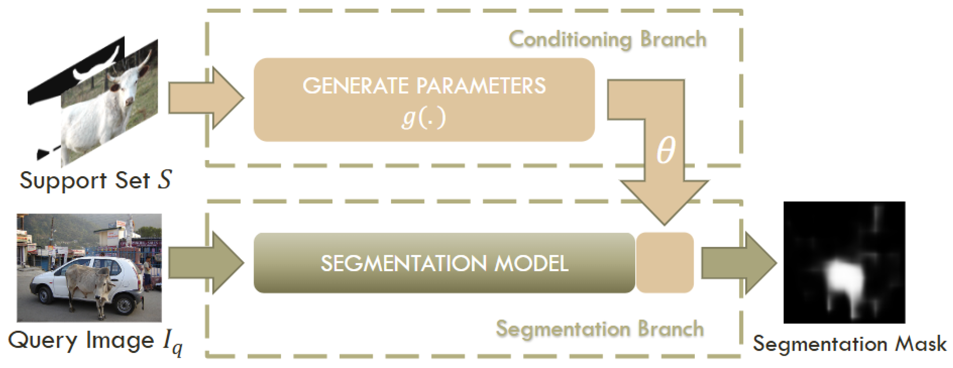
In 2017, Shaban et al. [24] designed a dual-branch model structure based on few-shot classification tasks, and introduced the idea of FSS for the first time, as shown in Figure 2 [24]. The model contains a condition branch and a segmentation branch. The conditional branch takes a set of support image-mask pairs as input, and extracts with VGGNet [25] features from it that are then passed to a function g ( ) , which outputs several parameters θ . The Segmentation Branch makes use of an FCN-32s model [26] to extract features from the query image, before the extracted features undergo an element-wise multiplication with the parameters θ produced by the conditional branch, thereby generating a segmented mask whose size corresponds to that of the input image after undergoing upsampling.
Similarly, co-FCN [27] has a double-branch architecture: the conditional branch deals with support set images, and the segmentation branch processes query set images. Conditional branches will connect images containing rich or sparse annotations by channel and encode them as features or parameters; then, the segmentation branch performs a dense segmentation in the above condition for the queried image. Contrary to OSLSM, co-FCN’s label division of support sets is different—with dense labels and sparse labels. Dense labels refer to binary mask images of the target object. Sparse labels only provide label values for a certain number of pixels in the image. In this phase, most studies see the task as a pixel classification problem and perform segmentation by training classifiers with marked images.

2.3. Prototype-Based Methods

The key to prototype-based methods is extracting the prototype for a class, usually the average of the feature vectors that support each category in an image. Most methods use masked average pooling to obtain a single prototype and then use some metrics to measure the similarity between the prototypes and the query. Representative algorithms: PLNet [28] and SGOne [29]. PLNet comes with the prototype-based few-shot segmentation architecture, inspired by some commonly used dual-branch architectures, depending on small sample classification and the prototype theory. The first branch is a prototype learner that outputs prototypes from a support set. The second branch is a segmentation network, which takes in the query image and prototypes and outputs a segmentation mask. Moreover, the author put forth the definition of N-way K-shot, with N-way denoting N categories and K-shot indicating the number of labeled examples in the query set. SG-One [29]’s model structure is shown as Figure 3 [29]. This study has analyzed different methods for the generation of prototypes. One is the multiplication between a binary mask and a support image to remove the pixel of the background, and the other is the concatenation between the support image with a positive and negative mask to create a block input composed of 5 channels. But there are drawbacks to both approaches. The first, which erases the background pixels to zero, changes the underlying statistical distribution of the supporting image set. The second, which links the support images back to their masks, breaks the network input structure. Based on this foundation, they propose Masked Average Pooling (MAP). The principle behind it is that a Fully Convolutional Network (FCN) keeps the relative positions between each and every pixel in an image that gets input into the network. As a result, the relevant feature is fully reserved after the multiplication of the binary mask and the extracted feature map, and the features from the backgrounds and other classes are excluded. This is a basic way to get support models out of the stuff being supported. It also uses cosine similarity to calculate the distance between the feature of the query and the feature of the support to guide the segmentation of the query images. Then, PANet [30] and CANet [31] used Masked Average Pooling.
There are also some methods that resolve one prototype not being enough in capturing spatial structures and details by using techniques like super pixel clustering or EM algorithms to produce several prototypes for modeling the similarities between different support images (labeled) and the query image (to segment). Representative methods include PGNet [32] and PMMs [33]. PGNet introduces the Graph Attention Mechanism to make use of graph structure to perform data modeling and also uses attentive graphs to pass on the label from the support set to the query set. The graph attention mechanism learns the attentions between connected graph nodes and builds an association between elements in the structured data. This allows each unlabeled pixel to select the relevant information from the supporting images. In order to capture correspondence at different semantic levels, the network designs a pyramid that models images of different scales as graph nodes and infers across different layers. Another way to improve is to use many prototypes and add to the prototype vector representation. The Prototype Mixture Model (PMM) solves the ambiguity of semantics when a single prototype is used on multiple segmentations of query images, which introduces a mixture model of prototypes. This can be seen from Figure 4 [33].

2.4. Matching-Based Methods

The above is the generation of a single prototype in previous work, and below is the network of multiple prototypes in PMMs. Each prototype represents a part of one target, and a different image region association is performed with the prototype, thereby strengthening the semantic representation based on prototypes. It can use several prototype vectors to represent a single prototype, in brief. Also, we have proposed a dual strategy whereby PMMs serve as representations and classifiers so as to activate spatial and channel semantics toward segmentation. To improve the representational power of the model, we stack a few PMMs so that it becomes a model ensemble, called Residual PPMS (RPMM). The first PPMM takes in the RGB image, and the last output will be fed as the supervision signal for the next query branch. This allows us to extract fine-grained segments progressively.
Another class of methods attempts to calculate similarity relationships between pixels in the support and query images, building a high-dimensional relational matrix for dense relational comparison. Representative algorithms such as HSNet [34]; DCAMA [35]. HSNet puts forward a hyper-correlation squeeze network that is based on multi-level feature correlations and effective 4D convolutions. The method takes features from different levels of the intermediate accumulation layer to build a set of 4D correlation tensors, which is called hyper-correlation. The reason why 4D convolution has a small-scale application is that it is not efficient. The proposed network uses a new way to make the weight of normal 4D convolution more efficient compared to the 4D convolution in [34]. In Figure 5, HSNet takes advantage of a central-axis 4D convolutional pyramid. It can continuously squeeze high-level semantic features together with low-level geometric cues from coarse-to-fine until producing accurate segmentation masks. DCAMA puts forward a method for dense-pixel level cross-querying, with an attention mechanism that gathers weighted post-masks supported by attention. In this framework, multi-level, per-pixel correlations of the whole foreground and background supportive information are applied to each query-support couple. The first step is using a pre-trained feature extraction network on the input image to obtain multi-scale query features and support features. At the same time, support masks are downscaled to a number of scales that correspond to image features. Secondly, the feature of queries, supporting features, and the support mask feature are sent into a multi-layer DCAMA block whose scales are the same as Q, K, and V, respectively, for multi-headed attention and query mask for aggregation. A bunch of query masks made from different scales are processed together with convolution, upsampling, and element-wise addition. Lastly, the output of the previous stage (multi-scale DCAMA) is connected to a multi-scale image feature through a skip connection and mixed using a mixer to form the final query mask. In short, such methods can effectively preserve the details of the image and all the structural elements, but they require lots of resources.

2.5. Methodology Utilizing Basic Models

In recent years, due to the constant development of general foundational models and pre-training techniques, more and more researchers have begun to focus on universal models in the visual field. It is not cost-effective to build a universal segmentor, so researchers often use pre-trained base models like SAM [36], CLIP [37], and the Stable Deffusion guardrail model [38] to significantly enhance the performance and generalization ability of segmentation tasks. Representative networks include CLIPSeg [39], SegGPT [40], DifFSS [41] et al.
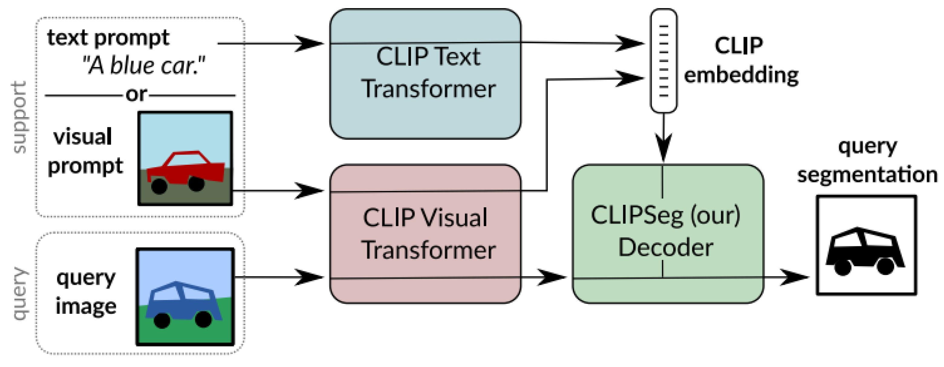
CLIPSeg can process both text and visual info at the same time, performing segmentation thanks to text questions or sample pics, and it does really well with referencing expression segmentation, zero-shot segmentation, and one-shot segmentation missions. The network architecture of the model is shown in Figure 6 [39] using a pre-trained CLIP model as backbone on top of which the decoder is trained. Full use of CLIP’s ability to process text and visual embedding space can handle the prompt in both text and images. Use a decoder to link internal activations in CLPP to output segmentation, making sure there is a minimal dataset bias and keeping CLIP’s great and wide ability to make predictions. CLIPSeg can take free-text prompts or a support set and generate binary segmentation masks for the query image. When only given descriptive information, the text encoder of CLP turns the description or the category’s name into a semantic prompt for the segmentation task. When just having the image as its information source, the image encoder of CLIP takes the support images and their mask to produce a visual prompt for the segmentation task. PGMA-Net [42] uses the CLIP model to propose the prior-knowledge-guided mask combination network, which embeds class-agnostic prior knowledge into the mask combination process to include text. And it helps mitigate the training bias toward the base classes, as was reported in other works. First, they introduced a Prior-Guided Mask Assembl Module (PGMAM) that uses affinities to assemble priors. It standardizes many different sorts of tasks via all sorts of different plug-and-play interactions between priors (i.e., visual elements, text elements, supporting elements, and querying elements) and affinities (interimage affinities, intraimage affinities, not training affinities, higher order affinities). With HDCDM, it is possible to use a single set of pattern weights for all tasks.
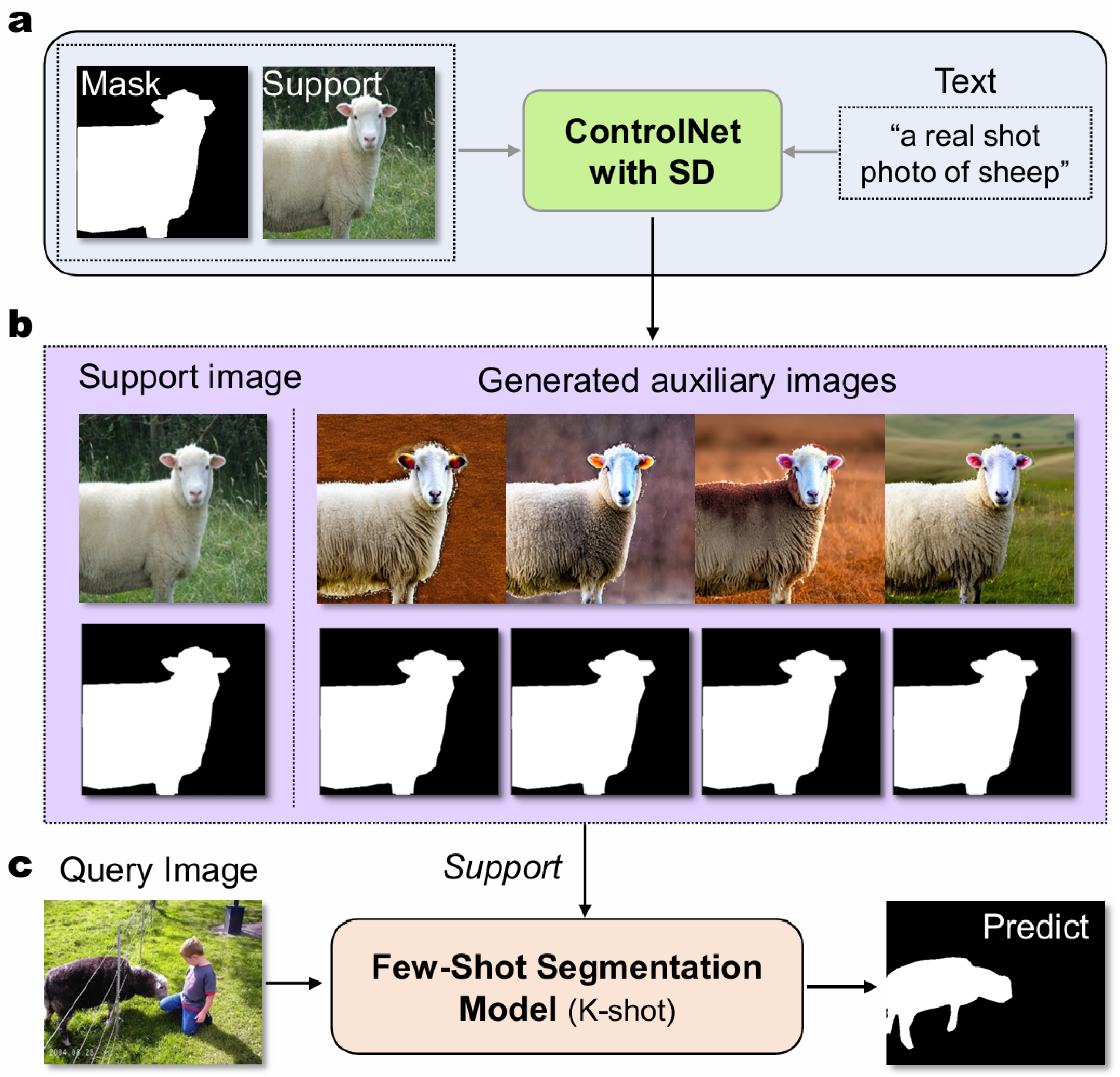
In addition to applying CLIP models, researchers also put forward some methods that could improve segmentation accuracy by means of Stable Diffusion models. As illustrated in Figure 7 [41], the diffusion model is a generative model that produces images by iteratively removing noise from noisy samples. DifFSS [41] is a new type of FSS architecture that centers around the concept of making a larger number of positive supporting images by utilizing diffusion models to create auxiliary images. The model uses the power of the Stable Diffusion model’s generation capabilities to generate all kinds of auxiliary support images according to the specified semantic masks, sketches, or soft HED boundaries as the control condition. The FSS model can refer to more kinds of support images, which will generate stronger representations and improve the performance of segmentation. The model improves the performance of semantic segmentation with auxiliary images generated in order to make the most of limited labeled information. Secondly, since the production of auxiliary pictures depends on the diffusion model, the diffusion model has good generality and can be used for different semantic segmentation situations. Furthermore, through visualization of the produced auxiliary images, people may obtain a more intuitive recognition of how the model works and thus increase their understanding of it.

3. Scene Challenge Analysis

Due to the different shooting heights of UAVs, there are significant variations in image scales. Affected by the inherent growth characteristics of coastal zone vegetation, there is high similarity between different categories, and the mixed contours of vegetation are difficult to distinguish. These pose great challenges to the in-depth analysis of images. This section will conduct an in-depth analysis of the difficulties in few-shot semantic segmentation on UAV coastal zone images, aiming at the characteristics of coastal zone data.

3.1. Segmentation Challenges Caused by UAV Imaging

Due to the high-altitude imaging method of UAVs, the size and scale of coastal vegetation change with the UAV’s altitude. When the vegetation is farther from the UAV, its scale is closer to the real-world proportions but appears smaller in size; when the vegetation is closer to the UAV, its size becomes larger, though it suffers from a certain degree of distortion in scale. Images of coastal vegetation captured from various angles and altitudes by UAVs exhibit significant variation in scale and size, even for the same species, leading to inconsistencies in morphological features.
As shown in Figure 8, (a) the image displays Spartina captured at a near focal length, clearly showing the detailed features of the leaves, while (b) the image, taken at a far focal length, illustrates the distribution characteristics of the plant population. This indicates that images taken at different focal lengths are required to comprehensively represent the various dimensional features of coastal vegetation, but it also introduces new challenges to semantic segmentation tasks.

3.2. Segmentation Challenges Arising from Vegetation Characteristics

Another significant challenge in the segmentation of coastal vegetation is the high inter-class similarity, which makes it difficult to distinguish target objects from the background. Figure 9 presents an image where Spartina coexists with other terrestrial vegetation. The red circles indicate Spartina, while the rectangles denote other plant species. As observed, at high-altitude imaging, both exhibit similar colors and morphologies, making them hard to differentiate. This often leads to the misclassification of background vegetation as the target category during the segmentation of Spartina. Although the coastal zone features a rich diversity of vegetation species, the similarities in their growth environments contribute to morphological resemblances among different species. Combined with the visual diversity caused by varying shooting angles and altitudes, it becomes even more challenging to distinguish among different types of vegetation.
Additionally, the coastal zone vegetation is characterized by mixed-species growth and blurred boundaries, posing considerable challenges for precise image segmentation. As shown in Figure 10, (a) the image labels four types of vegetation with the numbers 1, 2, 3, and 4, representing Reed, Spartina, Suaeda, and Tamarix, respectively. Among these, Reed, Spartina, and Tamarix exhibit similar color characteristics. Their interwoven growth patterns, coupled with varied and undulating terrain, significantly increase the complexity of automatic vegetation type recognition and segmentation. (b) The image identifies the distribution of Reed and Tamarix with the numbers 1 and 2. It clearly depicts a mixed-growth scenario where Tamarix and Reed coexist. The transitional zones between the two lack distinct boundaries, resulting in ambiguous edges that are difficult to delineate even through manual interpretation. This indistinct boundary feature imposes more stringent requirements on automated segmentation algorithms.

3.3. Visualization Analysis

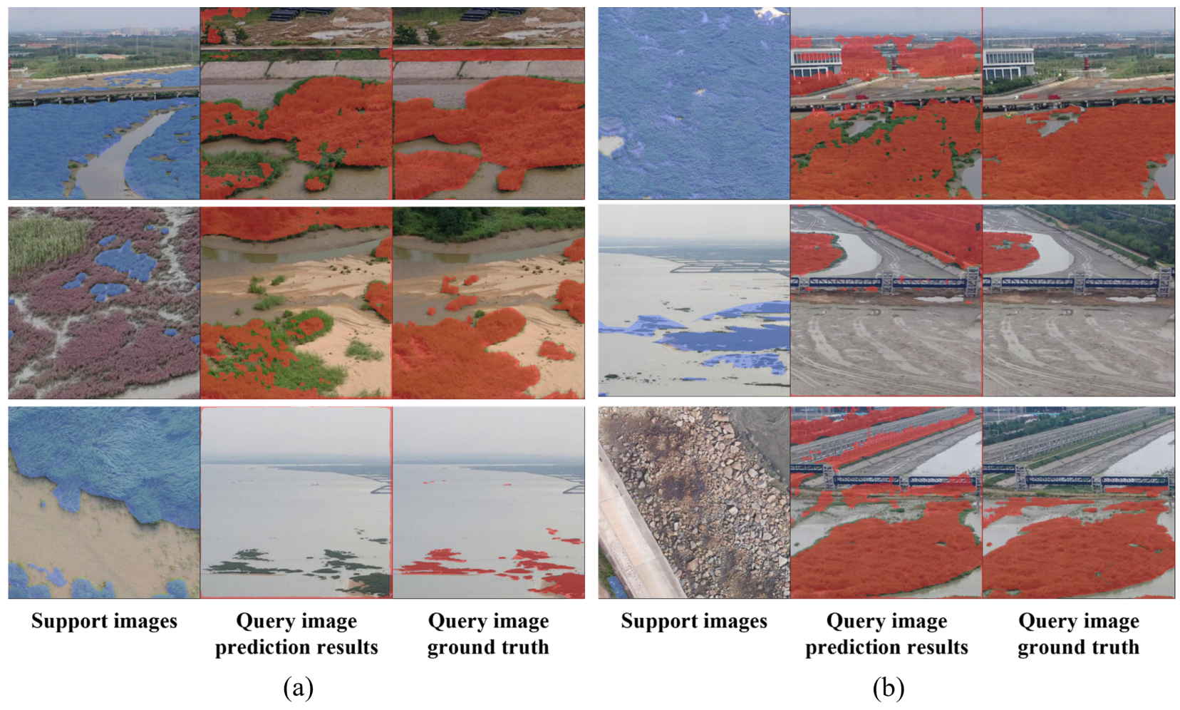
Experiments were conducted on the coastal dataset using the HSNet algorithm, with Spartina as the target class. The visualization results are shown in Figure 11. The first column displays the support images, where the blue mask indicates the Spartina class. The second column shows the query images, with red representing the segmentation results for Spartina. In the third column, red denotes the ground truth of Spartina in the query images.
(a) illustrates the segmentation challenges caused by UAV imaging. Due to variations in UAV shooting altitude, there are significant scale differences between the support and query images, resulting in suboptimal segmentation of Spartina in the query image, where some pixels remain unrecognized. This indicates that directly applying existing FSS methods fails to effectively capture multi-scale features, leading to poor performance when segmenting instances of the same class with significant scale variations. To ensure segmentation accuracy and identify multi-scale target objects, it is necessary to acquire contextual information at different scales and treat features with identical semantic information but varying sizes equally.
(b) demonstrates the segmentation difficulties arising from the intrinsic characteristics of coastal vegetation. When the query image contains both Spartina and visually similar vegetation types, background vegetation is often mistakenly classified as Spartina, resulting in inaccurate segmentation. Prototype-based FSS networks typically use masked average pooling when extracting prototypes, which can lead to the loss of detailed spatial information. Therefore, it is essential to establish a more tightly coupled visual correspondence between the support and query pairs to accurately identify pixels in the query image that belong to the target class.

4. Suggested Approach

To address the unique challenges in coastal imagery, such as scale variation, mixed vegetation growth, and blurred contours, this section proposes an FSS algorithm based on the Segment Anything Model (SAM). Building upon the meta-learner and base-learner integration strategy discussed in Section 3 for general scenarios, the algorithm introduces adaptive modifications to the meta-learner to accommodate the specific characteristics of coastal environments. Additionally, the SAM model is incorporated to enhance segmentation accuracy. The following subsections provide a detailed explanation of the overall algorithm framework and its key improvement modules.

4.1. Overall Suggested Approach Framework

This section elaborates on the proposed framework for FSS. The overall architecture is illustrated in Figure 12. The core concept of the framework lies in integrating an FSS algorithm with a pre-trained SAM to achieve accurate semantic segmentation of coastal imagery.
The framework takes as input the support images, support masks, and query images. These inputs are first fed into the FSS algorithm to predict a mask for the query image. However, conventional FSS methods perform poorly when applied directly to coastal images. Therefore, targeted enhancements have been made to improve the algorithm’s adaptability to the unique characteristics of coastal environments. Subsequently, the coarse mask generated by the FSS is used as a prompt and, together with the query image, is input into the pre-trained SAM model. Leveraging its powerful feature extraction capabilities, the SAM model captures fine-grained image details and produces a more accurate segmentation result. To further refine the output, a selection algorithm is introduced to filter and determine the final predicted result from the SAM outputs. The framework operates in inference mode, with the parameters of both the FSS algorithm and the SAM model frozen to ensure stability and consistency. To validate the effectiveness of the proposed framework, extensive experiments were conducted on a self-constructed UAV coastal image FSS dataset. The results demonstrate that the proposed framework performs exceptionally well in coastal image segmentation tasks and significantly outperforms existing few-shot segmentation methods.
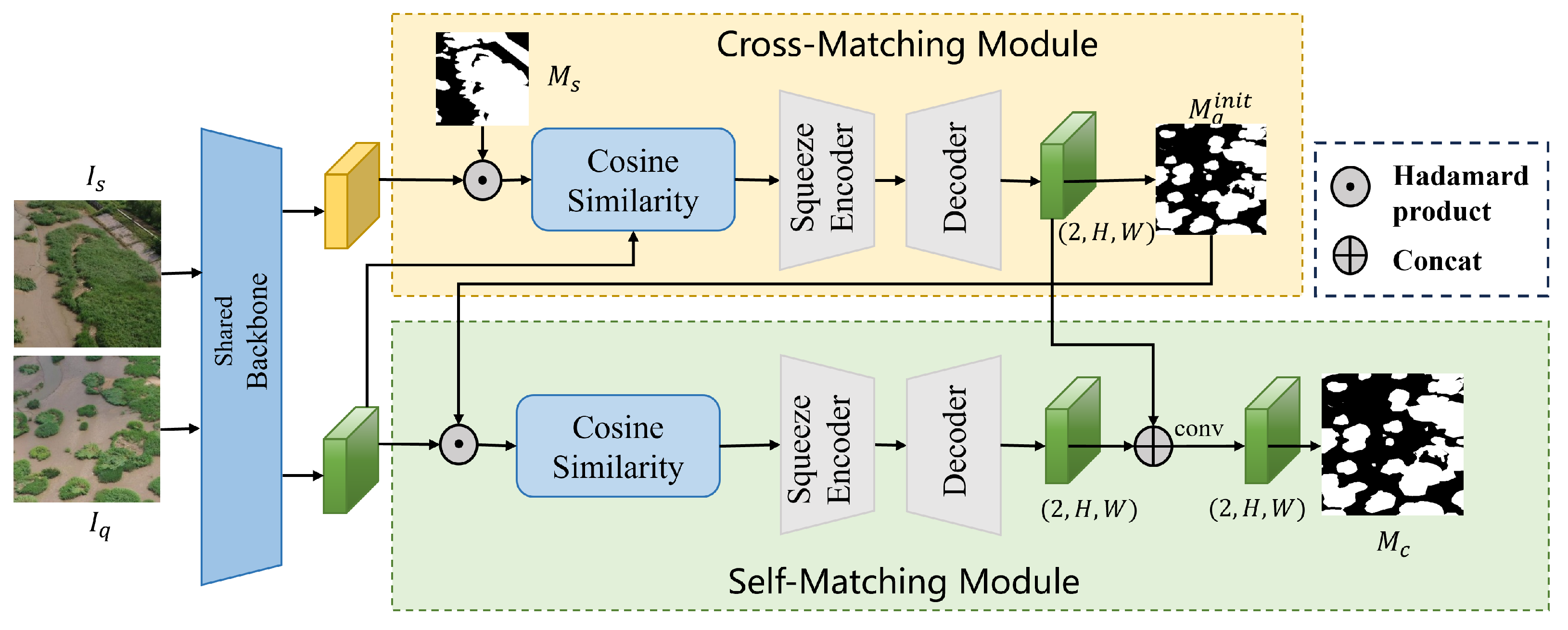
Figure 13 illustrates the framework of the meta-learner component of the FSS algorithm proposed in this study. It adopts a shared-weight backbone network to extract both support and query features. Based on the meta-learner structure designed for general scenarios, the hybrid prototype generation module is removed, and two new modules are introduced: the Cross-Matching Module (CMM) and the Self-Matching Module (SMM). First, the support features, support masks, and query features are fed into the CMM, which processes them to generate an initial query mask. This mask is then passed into the SMM, where the query features undergo a self-matching process, resulting in a coarse prediction output.

4.2. Cross-Matching Module

Unlike traditional approaches that encode annotated support images into fixed feature vectors to guide the segmentation of query images, this section proposes a pixel-level correlation-based segmentation strategy within the meta-learner. This strategy is specifically designed to address the dominance of vegetation classes and the high inter-class similarity in coastal imagery. In the Cross-Matching Module, cosine similarity is employed to compute the pixel-level correlation between the query image and the support image, aiming to capture their semantic associations. However, conventional correlation computation methods often yield similar cosine similarity values when dealing with visually similar classes, leading to segmentation errors. To overcome this issue, a Hyper-Correlation Pyramid structure is introduced into the Cross-Matching Module. This structure enhances the robustness and granularity of visual correspondences between the support and query images through multi-scale feature fusion and hierarchical correlation computation. Specifically, the Hyper-Correlation Pyramid first extracts features from both the support and query images at multiple scales. It then performs correlation calculations layer by layer, progressively refining the pixel-level matching results. This multi-level correlation approach not only improves the model’s ability to distinguish intra-class variations but also effectively mitigates confusion between similar classes, thereby significantly enhancing segmentation accuracy.
First, given a pair of query and support images, I q and I s , a pre-trained backbone network with shared weights is used to generate a series of feature maps, denoted as { ( F q l , F s l ) } l = 1 L . Among them, F q l and F s l represent the feature maps of the query and support images, respectively, at layer l. The support mask M s is then applied to encode the segmentation information and filter out background content, resulting in a masked support feature:
F ^ s l = F s l ζ l ( M s ) ,
here, ⊙ denotes the Hadamard product, and ζ l : R H × W R C i × H i × W i represents the operation of resizing the given tensor along the channel dimension at layer l.
Next, following the Hyper-Correlation Pyramid structure described in HSNet [34], for each layer, given a pair of feature maps F s l and F ^ s l , a 4D correlation tensor C l R H l × W l × H l × W l is used to compute the cosine similarity as follows:
C ^ l ( x q , x s ) = ReLU F q l ( x q ) · F ^ s l ( x s ) F q l ( x q ) F ^ s l ( x s ) ,
here, x q and x s represent the 2D spatial positions of the query and support feature maps, respectively, and ReLU is applied to suppress noisy correlation scores. From the resulting 4D correlation set { C ^ l } l = 1 L , if they share the same spatial dimensions, the subset is denoted as { C ^ l } l L p , where L p is a subset of CNN layer indices { 1 , . . . , L } in a certain pyramid layer p. All 4D tensors in { C ^ l } l L p are concatenated along the channel dimension to form the hyper-correlation tensor C p R | L p | × H p × W p × H p × W p , where ( H p , W p , H p , W p ) represents the spatial resolution of the hyper-correlation at pyramid level p. Given p pyramid levels, the hyper-correlation pyramid is denoted as C = { C p } p = 1 P , representing a rich set of feature correlations from multiple visual perspectives.
The hyper-correlation pyramid is then fed into a Hyper-Correlation Squeeze Encoder. The encoder network compresses it into a compact feature map, denoted as Z R 128 × H 1 × W 1 .
As shown in Figure 14, a sequence of multi-channel 4D convolutions with large strides periodically compresses the last two (support) spatial dimensions of C ^ p to ( H , W ) , while maintaining the first two (query) spatial dimensions at ( H p , W p ) . This process compresses the hyper-correlation pyramid into R 128 × H p × W p × H × W .
Similar to the structure in FPN [43], outputs from two adjacent pyramid levels, p and p + 1 , are merged by first upsampling the spatial dimensions (query) of the upper level by a factor of two, followed by element-wise addition. Subsequently, the merged output is processed with 4D convolution to propagate correlation information in a top-down manner to the lower levels. After iterative propagation, the output tensor from the smallest convolutional block is further compressed by applying average pooling over its last two (support) spatial dimensions. This yields a low-dimensional feature map D, which serves as the compressed representation of the hyper-correlation pyramid Z R 128 × H 1 × W 1 .
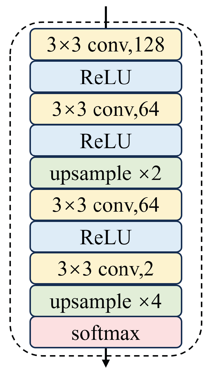
The structure of the decoder is shown in Figure 15. It employs a 2D convolutional context decoder composed of a series of 2D convolutional layers, ReLU activations, upsampling layers, and a softmax function. The contextual representation is fed into the decoder, resulting in a two-channel prediction map M ^ q i n i t [ 0 , 1 ] 2 × H × W , where the two-channel values represent the probabilities of the foreground and background, respectively. The maximum channel value at each pixel location is then selected to generate the initial query mask M q i n i t { 0 , 1 } H × W .

4.3. Self-Matching Module

While the Cross-Matching Module effectively captures the complex correlations between support and query images, addressing the issue of high similarity among vegetation classes in coastal regions, it remains challenged by significant intra-class scale variations, which are common due to UAV imaging methods. When the support image is captured at a far focal length and the query image at a close focal length, the support image may fail to convey detailed features of the target object, such as the leaf morphology of Spartina. Conversely, if the support image is taken at a close focal length and the query image at a far focal length, the support image may not provide insights into the object’s spatial distribution, such as Spartina’s clustered, elliptical formation. To mitigate the impact of scale discrepancies between support and query images, a Self-Matching Module is designed. This module leverages the intrinsic features of the query image itself as auxiliary support information for segmenting the query image.
Assume the query image is denoted as I q , and the initial query mask as M q i n i t . In the Self-Matching Module, instead of computing a correlation tensor between masked support features and query features, the correlation is calculated using the query features themselves. Specifically, a correlation tensor is computed between the initial masked query features and the query features:
C ^ l s e l f ( x q , x ^ q ) = ReLU F l q ( x q ) · F ^ l q ( x ^ q ) F l q ( x q ) F ^ l q ( x ^ q ) ,
where,
F ^ q l = F q l ζ l ( M i n i t q ) ,
following the procedure used in the Cross-Matching Module, tensor M ^ q s e l f [ 0 , 1 ] 2 × H × W can be obtained. Then, M ^ q s e l f and M ^ q i n i t are concatenated and passed through a 1 × 1 convolution to reduce the channel dimensionality, resulting in M ^ c [ 0 , 1 ] 2 × H × W . The maximum channel value at each pixel location is then selected to produce the meta-learner’s coarse prediction, M c { 0 , 1 } H × W . This coarse prediction, M c , is then combined with the base class prediction from the base learner to eliminate the influence of base classes, resulting in M f c .
The loss function, Loss, used for training the model, can be computed as follows:
L m = B C E ( M f c , M q ) ,
here, BCE(,) denotes the Binary Cross-Entropy loss [44], and M q is the ground truth mask of the query image. Since the quality of the initial predicted query mask directly affects the auxiliary information extracted during the self-matching stage, a Query Self-Matching Loss is proposed to further enhance the self-matching process:
L a u x = B C E M ^ a u x , M q ,
here, M a u x is generated in the same manner as M a u x , except that it uses the ground truth query mask to compute the masked query features. In other words, Equation (4) is replaced with
F ^ q l = F q l ζ l ( M q ) .
Finally, these two components are combined:
L = L m + λ L a u x .
The model is trained in an end-to-end manner, where λ is used as a weighting factor, and λ = 1.0, which has been confirmed by several related works to be typically chosen as the default value, is set in the experiments [45].

4.4. Refinement Using SAM

In coastal imagery, the presence of mixed vegetation, irregular edges, and complex object contours poses significant challenges for precise segmentation. Given the limited annotated data available for FSS methods, enhancing the internal structure of the model alone is often insufficient to achieve satisfactory contour segmentation results. Recently, the SAM [36], a large foundational segmentation model, has demonstrated strong performance in handling fine-grained details. Therefore, this study leverages SAM’s detail-refinement capabilities to enhance the segmentation output of the FSS network.
SAM, developed by Meta, is a powerful image segmentation model designed for general-purpose segmentation tasks. It exhibits robust generalization capabilities, enabling efficient segmentation across a wide range of scenarios and tasks, including but not limited to the automatic segmentation of objects, regions, and scenes. However, part of SAM’s impressive performance stems from its pre-training on large-scale datasets—conditions that are difficult to replicate in coastal areas due to the challenges in acquiring extensive image data. Moreover, SAM’s complex model architecture demands substantial computational resources during training. A straightforward approach to integrating SAM with FSS would be to re-implement SAM within the FSS framework and fine-tune it on the FSS dataset. However, this would entail significant computational costs. Instead of re-implementation and fine-tuning, this study adopts a training-free method that can effectively enhance FSS performance. This approach requires no additional training and can be seamlessly integrated into existing FSS methods.
As shown in Figure 12, this study utilizes SAM’s prompt engineering capabilities to perform post-processing on FSS results. The prediction result M f c , obtained from the FSS method, is used to generate the point and box prompts required by SAM. These generated prompts, together with the query image I q , are then input into SAM. Finally, the pre-trained SAM performs inference to produce a refined mask M s a m . However, due to the complexity of coastal scenes—particularly in images containing multiple objects—incorrect coarse predictions may occur, leading to erroneous point and box prompts. Specifically, there are three scenarios:
(1).
FSS predicts correctly, SAM predicts correctly: In this case, the prediction M s a m outperforms M f c in terms of accuracy.
(2).
FSS predicts correctly, SAM predicts incorrectly: Here, M s a m performs worse than M f c . This situation can be mitigated.
(3).
FSS predicts incorrectly: FSS predicts the wrong location for the target object. Consequently, the generated prompts are invalid, and the corresponding SAM output M s a m is also not useful.
Based on the three scenarios, the objective of this study is to enhance overall performance by reducing the occurrence of case (2). To achieve this, a selection mechanism is introduced to filter out erroneous predictions. Experimental results indicate that when M s a m and the corresponding M f c share a large number of pixels, the prediction is more likely to be accurate, and vice versa. A threshold value T = 0.75 is set. When the Intersection over Union (IoU) between M s a m and M f c exceeds T, M s a m is selected as the final prediction M f .
To verify the rationality of the selection for the threshold value T, we also conducted an ablation study to compare different values of T under both 1-shot and 5-shot settings. The results are summarized in Table 1 below:
As can be seen, T = 0.75 consistently achieves the best performance in both 1-shot and 5-shot scenarios, outperforming neighboring values (0.65 and 0.85). This empirical verification confirms that our chosen setting is optimal.

5. Experiment and Evaluation

Based on the algorithm design presented in the previous section, this section focuses primarily on demonstrating the effectiveness of the algorithm and empirically validating the value of the dataset. The following subsections will provide a detailed introduction to the dataset and experiments.

5.1. Dataset Description

The OUC-UAV-SEG dataset [8] is constructed based on images captured by UAV, including data from the coastal zone of the Liaohe Estuary, the estuary of the West Coast, and the Yellow River Estuary. A total of 1612 images are included. The dataset consists of 15 categories.
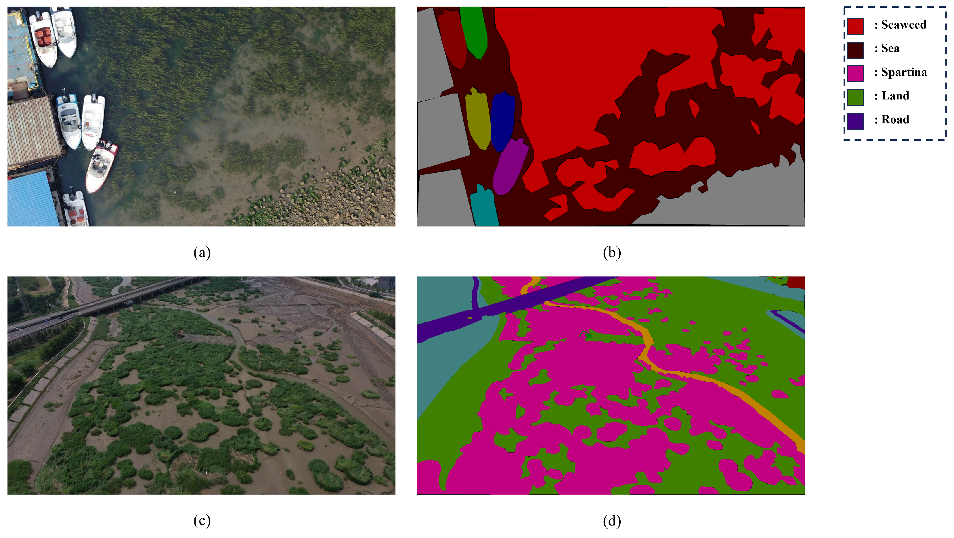
The dataset comprises the following categories: person, car, boat, Spartina, seaweed, reed, Tamarix, Suaeda, other vegetation, land, road, sea, sky, river, and building. Annotation was conducted using the LabelMe tool, with labels saved in JSON format. These JSON-format annotations were then converted into PNG format. The visualization of the images and their corresponding annotations is shown in Figure 16.
However, the original dataset cannot be directly used for FSS research. Therefore, this study constructed the OUC-UAV-SEG- 2 i dataset based on OUC-UAV-SEG. Six categories of interest—Spartina, Suaeda, reed, Tamarix, seaweed, and other vegetation—were selected as target classes, while all other categories were designated as background. The visualization of the images and their annotations is shown in Figure 17.
Subsequently, the images and their annotations were cropped to a uniform size of 473 × 473 pixels. The cropped images were then filtered to remove those that did not contain any target category objects. The remaining images were divided into a training set (11,984 images) and a validation set (3330 images). The dataset was further split into three folds based on category, with corresponding list files generated for each fold and saved in TXT format. Table 2 provides a breakdown of the fold composition in the constructed OUC-UAV-SEG- 2 i dataset. Each fold contains two categories, collectively covering the six primary vegetation classes found in coastal data. The first fold includes Spartina and Suaeda; the second fold includes Tamarix and reed; and the third fold consists of seaweed and other vegetation.

5.2. Experimental Details

The experiments were conducted on the same hardware platform—a server equipped with 8 NVIDIA (Santa Clara, California, United States.) RTX 4090 GPUs—and the training environment remained consistent with previous experiments. Specifically, two folds were randomly selected for training, while the remaining fold was used for testing. The model was trained for 200 epochs, with a learning rate of 5 × 10 3 and a batch size of 4. Each testing session was repeated five times using five different random seeds. In each test, 1000 support-query image pairs were sampled, and the average of the five tests was taken as the final result. The evaluation metrics used in the experiments were standard for FSS: Mean Intersection over Union (mIoU) and Foreground and Background Intersection over Union (FB-IoU).

5.3. Comparative Experiments

The proposed algorithm is compared with other FSS networks to evaluate its performance. Experiments were conducted under both 1-shot and 5-shot settings using different backbone networks. The evaluation was carried out from both quantitative and qualitative perspectives.

5.3.1. Qualitative Experiments

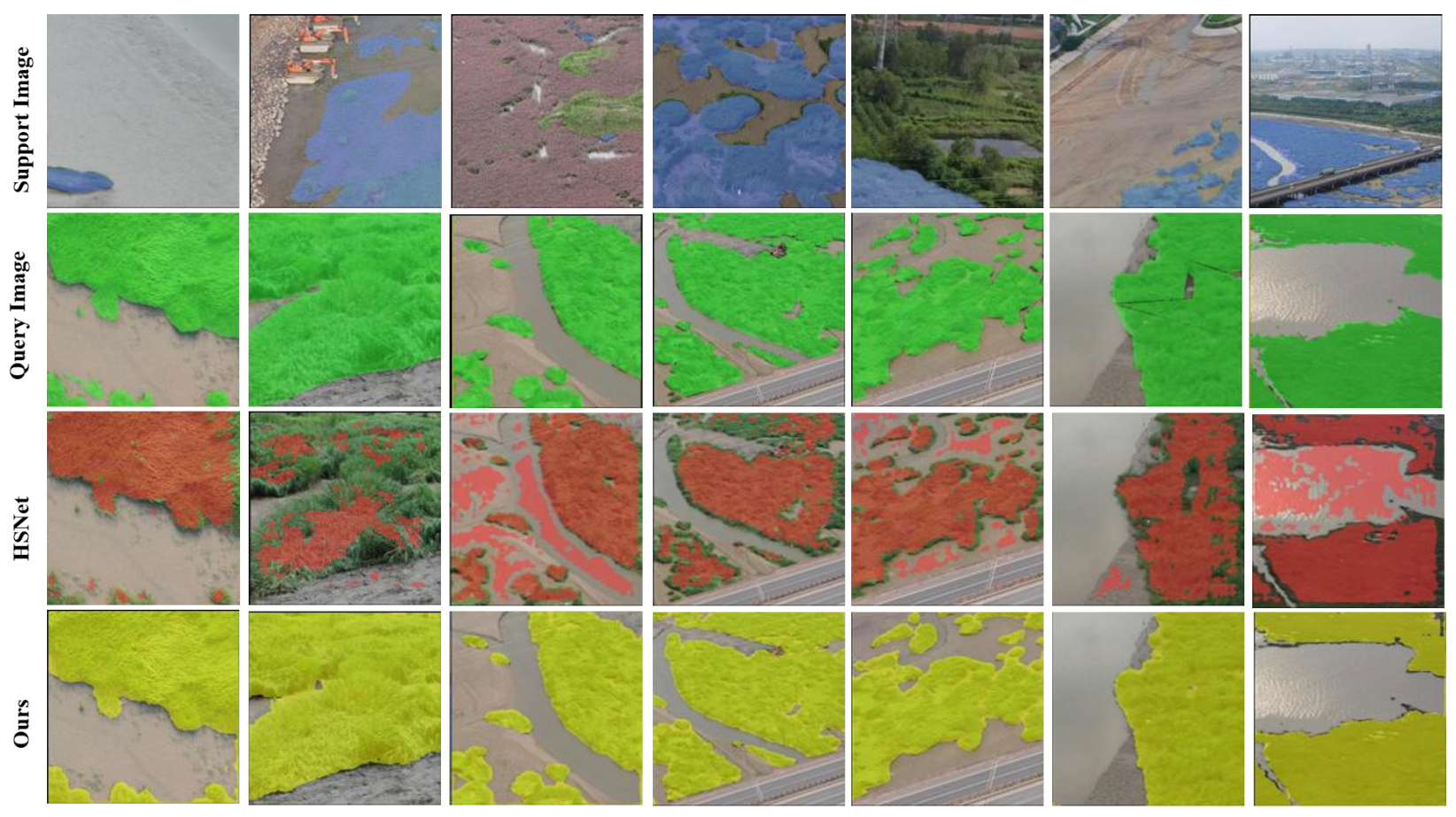
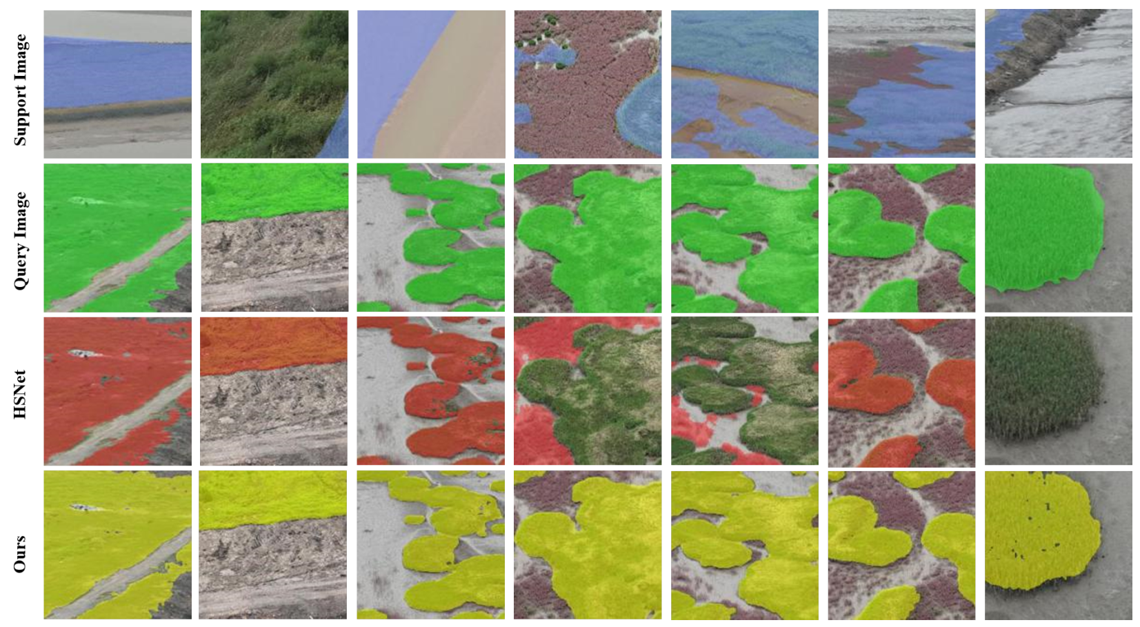
First, the qualitative results of the model are analyzed. The dataset includes six categories: Spartina, Suaeda, Tamarix, Reed, seaweeds, and other objects. One category from each fold was selected for visual result analysis. Figure 18 shows the visualization results of the Spartina category from the first fold under the 1-shot setting using the ResNet50 backbone network. The first row presents the support images of Spartina, with the target category marked in blue. The second row shows the query images, where the green area represents the ground-truth annotation of the target category (the category to be segmented). The third row displays the prediction results using the HSNet network, marked in red. The fourth row shows the prediction results of the proposed method, marked in yellow.
It can be observed that the proposed algorithm almost perfectly segments the target category, with results closely aligning with the ground truth annotations. Compared to the HSNet algorithm, it significantly improves issues such as incomplete segmentation regions and misclassification of other categories as the target category. Even in cases where there is a significant scale variation between the support and query images, the model still performs effectively. For instance, in the second column, the support image is taken from a high altitude, while the query image is captured from a lower altitude, resulting in a substantial scale difference. The algorithm successfully leverages the query image’s own information to assist in segmentation, maintaining strong performance. Additionally, the segmentation contours are smoother, indicating that the introduction of the general-purpose SAM model enhances detail refinement and enables more precise contour delineation of the target category.
Figure 19 presents the visualization results for the Reed category in the second fold under the 1-shot setting, using the ResNet50 backbone network. Similar to the structure in Figure 18, the first to fourth rows represent the support images, query images, HSNet prediction results, and the predictions generated by the proposed method, respectively.
In the visualizations of the first three columns, both the proposed method and the HSNet network successfully segment the target region. However, the proposed method yields clearer object contours and handles the edge regions with greater precision. The images in the fourth to sixth columns depict scenarios where Suaeda and Reed coexist. Due to their similar characteristics, HSNet misclassifies Suaeda as Reed. Although the sixth column shows correct segmentation, its contour processing is less refined compared to the proposed method. In the final column, significant scale differences exist between the query and support images due to differences in altitude and viewing angle. HSNet fails to identify the target region, whereas the proposed method almost accurately segments the Reed vegetation. This series of experiments demonstrates that the proposed method is better suited to handle segmentation challenges caused by scale variations in images. It more effectively leverages the information within the query image itself to guide segmentation, while also making full use of detailed spatial information to distinguish between visually similar vegetation types.
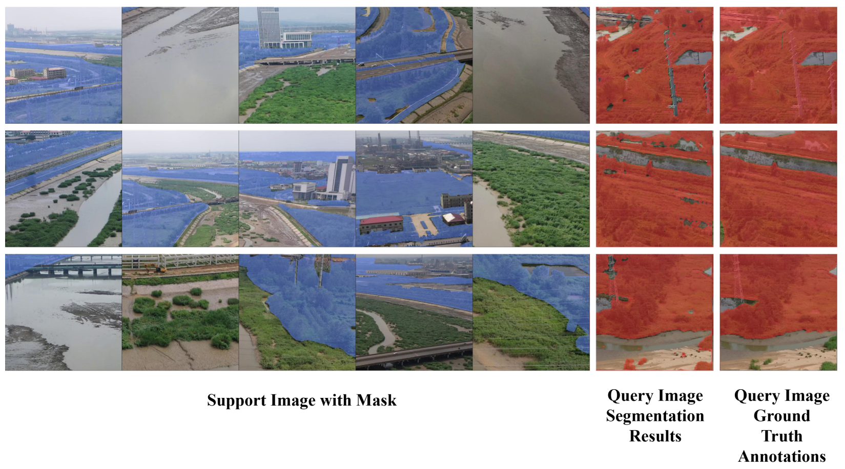
In addition to the 1-shot setting, experiments were also conducted under the 5-shot condition. Figure 20 shows the visualization results for the “other vegetation” category in the third fold, using five support images. The “other vegetation” category refers to vegetation types in coastal areas that are not part of the five main categories in the dataset. These may include vegetation growing near water, on the shore, or along roadsides, and encompass a wide variety of types, such as trees and grass clusters, which significantly increases the segmentation difficulty. Each row represents one combination. The first five columns display the five provided support images, with the target regions marked in blue. The sixth column presents the segmentation results produced by the proposed method, with the target areas marked in red. The seventh column shows the ground truth annotation of the query image, also marked in red. It is evident that even with the increased segmentation complexity, the use of multiple support images enables the proposed method to better address challenges posed by large image scale variations and complex mixed-vegetation scenarios, resulting in relatively accurate predictions of the target category.

5.3.2. Quantitative Experiments

While the qualitative visualization results demonstrate that the proposed method performs well in coastal scenarios, a more accurate assessment of its effectiveness requires a series of quantitative experiments.
Table 3 shows the performance comparison on the OUC-UAV-SEG- 2 i dataset using the ResNet50 backbone, with comparisons against PANet, CANet, PMMs, PFENet, HSNet, GenCo, POP, VP, and EKT. Bold values indicate the best performance, while underlined values represent the second-best. From the table structure, the first column specifies the backbone network used, i.e., ResNet50; the second column lists the competing methods, along with their sources and publication years in parentheses; the third to fifth columns present the mIoU values for three folds under the 1-shot setting, and the sixth column shows the average mIoU across the three folds. Similarly, the seventh to ninth columns display the mIoU values for the three folds under the 5-shot setting, and the final column reports the average mIoU in the 5-shot setting.
It is evident that the proposed method achieves superior performance across all settings, attaining the best results. Specifically, under the 1-shot and 5-shot settings, the proposed method reached average mIoU scores of 53.76% and 56.13%, respectively. Compared with the best existing methods, it achieved improvements of 4.69% and 4.50% in mIoU for the 1-shot and 5-shot settings, respectively, fully demonstrating the effectiveness and advantages of the proposed approach in FSS tasks. Further analyzing the performance across each fold, under the 1-shot setting, the proposed method achieved mIoU scores of 53.09%, 60.21%, and 47.97% on the first, second, and third folds, respectively, all of which were the highest. Under the 5-shot setting, the method achieved the best performance of 65.35% on the second fold and second-best performances of 55.54% and 47.52% on the first and third folds, respectively.
Notably, in the table, when comparing with the three methods of POP (CVPR 2023), VP (CVPR 2024), and EKT (AAAI 2025), the suggested approach consistently achieves the best performance under both 1-shot and 5-shot settings. Compared with the most recent state-of-the-art method, EKT (AAAI 2025), the suggested approach yields an absolute improvement of +2.86% (1-shot) and +2.13% (5-shot) on average across folds. This demonstrates that the suggested method not only incorporates the latest baseline comparisons but also achieves clear advances over them, further highlighting its effectiveness and novelty.
Based on the comprehensive analysis of the above experimental results, the proposed method has achieved the best performance in six metrics and the second-best performance in two metrics when compared with different models. This fully validates its robustness and superiority in conducting Few-Shot Segmentation (FSS) tasks in coastal scenarios.
By replacing the backbone network with ResNet101, comparative experiments were conducted with mainstream network models. The mIoU metrics under different settings are shown in Table 4, with the structure identical to that of Table 3. The results in the last row show that the proposed method achieved average mIoU scores of 55.25% and 60.52% under the 1-shot and 5-shot settings, respectively. Compared with the best existing methods, the mIoU of the proposed model improved by 1.2% and 1.8% under the 1-shot and 5-shot settings, respectively. Compared with the ResNet50 backbone, the mIoU values increased by 1.49% and 4.39% under the 1-shot and 5-shot settings, respectively.
Analyzing each fold in the dataset: on the first fold, the proposed method achieved the best performance of 53.09% under the 1-shot setting and the second-best performance of 55.54% under the 5-shot setting. On the second fold, the method achieved the best performances of 60.21% and 65.35% under both settings. On the third fold, it achieved the best performance of 47.97% under the 1-shot setting and the second-best performance of 47.52% under the 5-shot setting. Overall, the performance on the second fold was the most outstanding. In conclusion, the proposed method achieved the best performance and improved the segmentation accuracy of the target categories.
For the Foreground and Background Intersection over Union (FB-IoU) metric, the results on the OUC-UAV-SEG 2 i dataset are presented in Table 5, with the average value across the three folds used as the evaluation standard. The first column of the table lists the backbone networks, including both ResNet50 and ResNet101; the second column shows the methods used for comparison; and the third and fourth columns present the FB-IoU values under the 1-shot and 5-shot settings, respectively. The best-performing results are displayed in bold, while the second-best results are underlined.
It can be observed that the proposed model outperforms other methods when using both ResNet50 and ResNet101 as backbone networks. With ResNet50 as the backbone, the proposed method achieved Foreground-Background IoU scores of 66.21% and 69.05% under the 1-shot and 5-shot settings, respectively, showing improvements of 0.68% and 1.03% over the second-best method. When using ResNet101 as the backbone, the proposed method achieved FB-IoU scores of 67.83% and 70.62% under the 1-shot and 5-shot settings, respectively, outperforming the second-best method by 2.12% and 2.59%.

5.4. Ablation Study

To verify the effectiveness of the proposed network, extensive ablation experiments were conducted on the constructed coastal dataset OUC-UAV-SEG-2i. The study focused on evaluating the contributions of the CMM, the SMM, and the SAM model configured with the selection mechanism for refinement. All experiments were performed under the 1-shot setting, using ResNet50 as the feature extraction backbone. These ablation experiments offer an in-depth analysis of the impact of each component on overall performance and validate their effectiveness in FSS tasks. The experimental results are presented in Table 6.
First, the original HSNet network was trained and tested on the constructed dataset to obtain the mIoU for each category and the Mean mIoU. Then, the CMM and SMM were sequentially added, and the resulting coarse segmentation outputs were refined using the SAM model with a selection mechanism to determine the final segmentation results. The experimental results show that after adding the CMM module, the mIoU values for each category increased by 0.53%, 1.08%, and 0.85%, respectively, with the Mean mIoU improving by 0.82%. Upon incorporating the SMM module, the category-wise mIoU improved by 1.15%, 0.37%, and 1.64%, resulting in a 1.06% increase in the Mean mIoU. Based on this, after refinement using SAM (as shown in rows four and five), the mIoU values for each category further improved by 1.86%, 1.49%, and 2.09%, with the Mean mIoU increasing by 2.84%. Compared with the original network (i.e., the first row), the overall increase in Mean mIoU is 4.69%, thereby validating the effectiveness of each component.

6. Conclusions and Outlook

Vegetation classification and recognition in coastal zones are of great significance for preventing species invasion and protecting the ecological environment. However, coastal images are characterized by large-scale variations, high inter-class similarity among vegetation types, and mixed-species growth, all of which severely affect the accuracy of FSS. Based on the OUC-UAV-SEG coastal vegetation dataset, this study constructed the OUC-UAV-SEG- 2 i dataset and proposed an FSS network tailored for coastal scenarios, which integrates cross-matching and self-matching mechanisms.
This work not only provides critical data support for the study of FSS algorithms on UAV-captured coastal imagery but also lays the foundation for future related research. Future research directions can focus on developing lightweight base learners more suitable for this task, reducing model complexity while maintaining accuracy as much as possible, thereby suppressing the impact of base classes on prediction results and improving algorithm accuracy. In addition, in the future, we can continue to improve and supplement the existing dataset to enable it to fully play its role in research.

Author Contributions

Conceptualization, Y.W.; Methodology, Y.W.; Software, Y.W.; Validation, C.L.; Formal analysis, Z.G. and W.L.; Investigation, Z.G.; Data curation, Z.G. and W.L.; Writing—original draft, Y.W. and C.L.; Writing—review & editing, C.L., W.L. and S.W.; Visualization, Z.G.; Supervision, S.W. All authors have read and agreed to the published version of the manuscript.

Funding

This work was supported in part by the National Science Foundation of China under Grant 42476194, U24A20242, 62471448 and Grant 62102338; in part by Shandong Provincial Natural Science Foundation under Grant ZR2024YQ004, ZR2021ZD19 and No. ZR2024MF097; in part by TaiShan Scholars Youth Expert Program of Shandong Province under Grant tsqn202312109; in part by the Science and Technology Program of Qingdao (24-1-8-cspz-22-nsh).

Data Availability Statement

The original contributions presented in this study are included in the article. Further inquiries can be directed to the corresponding author.

Conflicts of Interest

The authors declare no conflicts of interest.

References

  1. Liu, Z.; Hu, F.; Xiao, K.; Chen, X.; Ye, S.; Sun, L.; Qin, S. Research Progress on the Delineation of Coastal Zone Scope and Boundaries. J. Appl. Oceanogr. 2025, 44, 15–20. [Google Scholar]
  2. Zhang, S. UAV-Based Research on Semantic Segmentation Methods for Coastal Zone Remote Sensing Images. Master’s Thesis, Liaoning Technical University, Fuxin, China, 2022. [Google Scholar]
  3. Jiang, X.; He, X.; Lin, M.; Gong, F.; Ye, X.; Pan, D. Advances in the Application of Marine Satellite Remote Sensing in China. Acta Oceanol. Sin. 2019, 41, 113–124. [Google Scholar]
  4. Li, X.; Li, X.; Liu, W.; Wei, B.; Xu, X. A UAV-based Framework for Crop Lodging Assessment. Eur. J. Agron. 2021, 123, 126201. [Google Scholar] [CrossRef]
  5. Ghassoun, Y.; Gerke, M.; Khedar, Y.; Backhaus, J.; Bobbe, M.; Meissner, H.; Tiwary, P.K.; Heyen, R. Implementation and Validation of a High Accuracy UAV-Photogrammetry Based Rail Track Inspection System. Remote Sens. 2021, 13, 384. [Google Scholar] [CrossRef]
  6. Dou, Y.; Yao, F.; Wang, X.; Qu, L.; Chen, L.; Xu, Z.; Ding, L.; Bullock, L.B.; Zhong, G.; Wang, S. PanopticUAV: Panoptic Segmentation of UAV Images for Marine Environment Monitoring. Comput. Model. Eng. Sci. 2024, 138, 1001–1014. [Google Scholar] [CrossRef]
  7. Liu, Y.; Yao, F.; Ding, L.; Xu, Z.; Yang, X.; Wang, S. An Image Segmentation Method Based on Transformer and Multi-Scale Feature Fusion for UAV Marine Environment Monitoring. In Proceedings of the 2023 8th International Conference on Image, Vision and Computing (ICIVC), Dalian, China, 27–29 July 2023; pp. 328–336. [Google Scholar] [CrossRef]
  8. Wang, S.; Wang, X.; Qu, L.; Yao, F.; Liu, Y.; Li, C.; Wang, Y.; Zhong, G. Semantic Segmentation Benchmark Dataset for Coastal Ecosystem Monitoring Based on Unmanned Aerial Vehicle (UAV). J. Image Graph. 2024, 29, 2162–2174. [Google Scholar] [CrossRef]
  9. Wang, S.; Wang, D.; Liang, Q.; Jin, Y.; Liu, L.; Zhang, T. Review on Few-Shot Learning. Space Control Technol. Appl. 2023, 49, 1–10. [Google Scholar]
  10. Li, K.; Chen, J.; Li, G.; Jiang, X. Survey on Research of Few-Shot Learning. Mech. Electr. Eng. Technol. 2023, 1–10. [Google Scholar]
  11. Ravi, S.; Larochelle, H. Optimization as a Model for Few-Shot Learning. In Proceedings of the International Conference on Learning Representations, Toulon, France, 24–26 April 2017. [Google Scholar]
  12. Finn, C.; Abbeel, P.; Levine, S. Model-Agnostic Meta-Learning for Fast Adaptation of Deep Networks. In Proceedings of the International Conference on Machine Learning, PMLR, Sydney, Australia, 6–11 August 2017; pp. 1126–1135. [Google Scholar]
  13. Antoniou, A.; Edwards, H.; Storkey, A. How to Train Your MAML. In Proceedings of the International Conference on Learning Representations, Vancouver, BC, Canada, 30 April–3 May 2018. [Google Scholar]
  14. Li, Z.; Zhou, F.; Chen, F.; Li, H. Meta-SGD: Learning to Learn Quickly for Few-Shot Learning. arXiv 2017, arXiv:1707.09835. [Google Scholar]
  15. Elsken, T.; Stafffer, B.; Metzen, J.H.; Hutter, F. Meta-Learning of Neural Architectures for Few-Shot Learning. In Proceedings of the IEEE/CVF Conference on Computer Vision and Pattern Recognition, Seattle, WA, USA, 13–19 June 2020; pp. 12365–12375. [Google Scholar]
  16. Graves, A. Neural Turing Machines. arXiv 2014, arXiv:1410.5401. [Google Scholar] [CrossRef]
  17. Cai, Q.; Pan, Y.; Yao, T.; Yan, C.; Mei, T. Memory Matching Networks for One-Shot Image Recognition. In Proceedings of the IEEE Conference on Computer Vision and Pattern Recognition, Salt Lake City, UT, USA, 18–23 June 2018; pp. 4080–4088. [Google Scholar]
  18. Munkhdalai, T.; Yuan, X.; Mehri, S.; Trischler, A. Rapid Adaptation with Conditionally Shifted Neurons. In Proceedings of the International Conference on Machine Learning, PMLR, Stockholm, Sweden, 10–15 July 2018; pp. 3664–3673. [Google Scholar]
  19. Kaiser, Ł.; Nachum, O.; Roy, A.; Bengio, S. Learning to Remember Rare Events. arXiv 2017, arXiv:1703.03129. [Google Scholar]
  20. Wei, T.; Li, X.; Liu, H. A Survey on Semantic Image Segmentation Under the Few—Shot Learning Dilemma. Comput. Eng. Appl. 2023, 59, 1–11. [Google Scholar]
  21. Koch, G.; Zemel, R.; Salakhutdinov, R. Siamese Neural Networks for One-Shot Image Recognition. In Proceedings of the ICML Deep Learning Workshop, Lille, France, 6–11 July 2015; Volume 2, pp. 1–30. [Google Scholar]
  22. Vinyals, O.; Blundell, C.; Lillicrap, T.; Kavukcuoglu, K.; Wierstra, D. Matching Networks for One-Shot Learning. In Proceedings of the Advances in Neural Information Processing Systems, Barcelona, Spain, 5–10 December 2016; Volume 29. [Google Scholar]
  23. Snell, J.; Swersky, K.; Zemel, R. Prototypical Networks for Few-Shot Learning. In Proceedings of the Advances in Neural Information Processing Systems, Long Beach, CA, USA, 4–9 December 2017; Volume 30. [Google Scholar]
  24. Shaban, A.; Bansal, S.; Liu, Z.; Essa, I.; Boots, B. One-Shot Learning for Semantic Segmentation. arXiv 2017, arXiv:1709.03410. [Google Scholar] [CrossRef]
  25. Simonyan, K.; Zisserman, A. Very Deep Convolutional Networks for Large-Scale Image Recognition. arXiv 2014, arXiv:1409.1556. [Google Scholar] [CrossRef]
  26. Long, J.; Shelhamer, E.; Darrell, T. Fully Convolutional Networks for Semantic Segmentation. In Proceedings of the IEEE Conference on Computer Vision and Pattern Recognition, Boston, MA, USA, 7–12 June 2015; pp. 3431–3440. [Google Scholar] [CrossRef]
  27. Rakelly, K.; Shelhamer, E.; Darrell, T.; Efros, A.; Levine, S. Conditional Networks for Few-Shot Semantic Segmentation. In Proceedings of the ICLR, Vancouver, BC, Canada, 30 April–3 May 2018. [Google Scholar]
  28. Dong, N.; Xing, E.P. Few-Shot Semantic Segmentation with Prototype Learning. In Proceedings of the British Machine Vision Conference, Newcastle, UK, 3–6 September 2018; Volume 3, p. 4. [Google Scholar]
  29. Zhang, X.; Wei, Y.; Yang, Y.; Huang, P. SG-One: Similarity Guidance Network for One-Shot Semantic Segmentation. IEEE Trans. Cybern. 2020, 50, 3855–3865. [Google Scholar] [CrossRef] [PubMed]
  30. Wang, K.; Liew, J.H.; Zou, Y.; Zhou, Y.; Feng, J. Panet: Few-Shot Image Semantic Segmentation with Prototype Alignment. In Proceedings of the IEEE/CVF International Conference on Computer Vision, Seoul, Republic of Korea, 27 October–2 November 2019; pp. 9197–9206. [Google Scholar] [CrossRef]
  31. Zhang, C.; Lin, G.; Liu, F.; Yao, T.; Shen, T. Canet: Class-Agnostic Segmentation Networks with Iterative Refinement and Attentive Few-Shot Learning. In Proceedings of the IEEE/CVF Conference on Computer Vision and Pattern Recognition, Long Beach, CA, USA, 15–20 June 2019; pp. 5217–5226. [Google Scholar] [CrossRef]
  32. Zhang, C.; Lin, G.; Liu, F.; Guo, J.; Wu, W.; Yao, T. Pyramid Graph Networks with Connection Attentions for Region-Based One-Shot Semantic Segmentation. In Proceedings of the IEEE/CVF International Conference on Computer Vision, Seoul, Republic of Korea, 27 October–2 November 2019; pp. 9587–9595. [Google Scholar] [CrossRef]
  33. Yang, B.; Liu, C.; Li, B.; Jiao, J.; Ye, Q. Prototype Mixture Models for Few-Shot Semantic Segmentation. In Proceedings of the Computer Vision—ECCV 2020: 16th European Conference, Glasgow, UK, 23–28 August 2020; Proceedings, Part VIII. Springer: Berlin/Heidelberg, Germany, 2020; pp. 763–778. [Google Scholar] [CrossRef]
  34. Min, J.; Kang, D.; Cho, M. Hypercorrelation Squeeze for Few-Shot Segmentation. In Proceedings of the IEEE/CVF International Conference on Computer Vision, Montreal, QC, Canada, 10–17 October 2021; pp. 6941–6952. [Google Scholar] [CrossRef]
  35. Shi, X.; Wei, D.; Zhang, Y.; Lu, J.; Ning, J.; Chen, Y.; Ma, J.; Zheng, Y. Dense Cross-Query-and-Support Attention Weighted Mask Aggregation for Few-Shot Segmentation. In Proceedings of the European Conference on Computer Vision, Tel Aviv, Israel, 23–27 October 2022; Springer: Berlin/Heidelberg, Germany, 2022; pp. 151–168. [Google Scholar] [CrossRef]
  36. Kirillov, A.; Mintun, E.; Ravi, N.; Mao, H.; Rolland, C.; Gustafson, L.; Xiao, T.; Whitehead, S.; Berg, A.C.; Lo, W.Y.; et al. Segment Anything. In Proceedings of the IEEE/CVF International Conference on Computer Vision, Paris, France, 1–6 October 2023; pp. 4015–4026. [Google Scholar]
  37. Radford, A.; Kim, J.W.; Hallacy, C.; Ramesh, A.; Goh, G.; Agarwal, S.; Sastry, S.; Askell, A.; Mishkin, P.; Clark, J.; et al. Learning Transferable Visual Models from Natural Language Supervision. In Proceedings of the International Conference on Machine Learning, PMLR, Virtual, 18–24 July 2021; pp. 8748–8763. [Google Scholar] [CrossRef]
  38. Rombach, R.; Blattmann, A.; Lorenz, D.; Esser, P.; Ommer, B. High-Resolution Image Synthesis with Latent Diffusion Models. arXiv 2022, arXiv:2112.10752. [Google Scholar] [CrossRef]
  39. Lüddecke, T.; Ecker, A.S. Image Segmentation Using Text and Image Prompts. arXiv 2022, arXiv:2112.10003. [Google Scholar] [CrossRef]
  40. Wang, X.; Zhang, X.; Cao, Y.; Wang, D.; Shen, T.; Huang, T. Seggpt: Segmenting Everything in Context. arXiv 2023, arXiv:2304.03284. [Google Scholar] [CrossRef]
  41. Tan, W.; Chen, S.; Yan, B. DiffSS: Diffusion Model for Few-Shot Semantic Segmentation. arXiv 2023, arXiv:2307.00773. [Google Scholar] [CrossRef]
  42. Chen, S.; Meng, F.; Zhang, R.; Qiu, H.; Li, H.; Wu, Q.; Xu, L. Visual and Textual Prior Guided Mask Assemble for Few-Shot Segmentation and Beyond. arXiv 2023, arXiv:2308.07539. [Google Scholar] [CrossRef]
  43. Lin, T.Y.; Dollár, P.; Girshick, R.; He, K.; Hariharan, B.; Belongie, S. Feature Pyramid Networks for Object Detection. In Proceedings of the IEEE Conference on Computer Vision and Pattern Recognition, Honolulu, HI, USA, 21–26 July 2017; pp. 2117–2125. [Google Scholar] [CrossRef]
  44. Hastie, T.; Tibshirani, R.; Friedman, J. Linear Methods for Classification. In The Elements of Statistical Learning: Data Mining, Inference, and Prediction, 2nd ed.; Springer: Berlin/Heidelberg, Germany, 2009; pp. 101–137. [Google Scholar]
  45. Ruder, S. An Overview of Multi-Task Learning in Deep Neural Networks. arXiv 2017, arXiv:1706.05098. [Google Scholar] [CrossRef]
  46. Tian, Z.; Zhao, H.; Shu, M.; Yang, L.; Li, X.; Jia, J. Prior Guided Feature Enrichment Network for Few-Shot Segmentation. arXiv 2020, arXiv:2008.01449. [Google Scholar] [CrossRef] [PubMed]
  47. Wu, J.; Hovakimyan, N.; Hobbs, J. Genco: An Auxiliary Generator from Contrastive Learning for Enhanced Few-Shot Learning in Remote Sensing. In ECAI 2023; IOS Press: Amsterdam, The Netherlands, 2023. [Google Scholar]
  48. Naik, H.; Chan, A.H.H.; Yang, J.; Delacoux, M.; Couzin, I.D.; Kano, F.; Nagy, M. 3D-POP—An Automated Annotation Approach to Facilitate Markerless 2D-3D Tracking of Freely Moving Birds with Marker-based Motion Capture. arXiv 2023, arXiv:2303.13174. [Google Scholar] [CrossRef]
  49. Chen, Y.; Pant, Y.; Yang, H.; Yao, T.; Meit, T. VP3D: Unleashing 2D Visual Prompt for Text-to-3D Generation. In Proceedings of the 2024 IEEE/CVF Conference on Computer Vision and Pattern Recognition (CVPR), Seattle, WA, USA, 16–22 June 2024. [Google Scholar]
  50. Chen, X.; Shi, M.; Zhou, Z.; He, L.; Tsoka, S. Enhancing Generalized Few-Shot Semantic Segmentation via Effective Knowledge Transfer. In Proceedings of the AAAI Conference on Artificial Intelligence (AAAI), Philadelphia, PA, USA, 25 February–4 March 2025. [Google Scholar]
  51. Xu, Q.; Zhao, W.; Lin, G.; Long, Y. Self-Calibrated Cross Attention Network for Few-Shot Segmentation. In Proceedings of the IEEE/CVF International Conference on Computer Vision, Paris, France, 1–6 October 2023; pp. 655–665. [Google Scholar] [CrossRef]
  52. Liu, H.; Peng, P.; Chen, T.; Wang, X.; Yao, Y.; Hua, Z. Fecanet: Boosting few-shot semantic segmentation with feature-enhanced context-aware network. IEEE Trans. Multimed. 2023, 25, 8580–8592. [Google Scholar] [CrossRef]
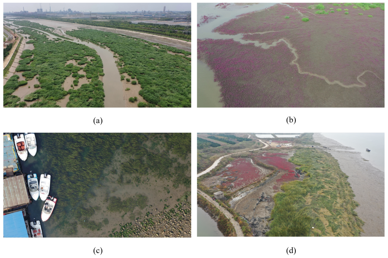
Figure 1. Example aerial images from the UAV-OUC-SEG dataset: (a): Spartina alterniflora; (b): Suaeda salsa; (c): seagrass bed; (d): reeds.
Remotesensing 17 03404 g001
Figure 2. Schematic diagram of the OSLSM network model.
Remotesensing 17 03404 g002
Figure 3. Schematic diagram of the SG-One network model.
Remotesensing 17 03404 g003
Figure 4. Schematic diagram comparing a single prototype network with multiple prototype networks.
Remotesensing 17 03404 g004
Figure 5. Schematic diagram of the principle of efficient 4D convolution.
Remotesensing 17 03404 g005
Figure 6. Schematic diagram of the CLIPSeg network model.
Remotesensing 17 03404 g006
Figure 7. Schematic diagram of the DifFSS network model. (ac): Multi-stage denoising is performed using noise samples, and finally the image is generated.
Remotesensing 17 03404 g007
Figure 8. Spartina captured by UAV at different focal lengths.
Remotesensing 17 03404 g008
Figure 9. (a,b) High similarity between Spartina and other vegetation, Circles: Spartina, Rectangles: Other plants.
Remotesensing 17 03404 g009
Figure 10. (a,b) Phenomenon of mixed vegetation growth.
Remotesensing 17 03404 g010
Figure 11. (a,b) Visualization of segmentation results for Spartina using existing algorithms.
Remotesensing 17 03404 g011
Figure 12. Framework of the FSS algorithm for coastal imagery.
Remotesensing 17 03404 g012
Figure 13. Structure of the FSS algorithm with CMM and SMM.
Remotesensing 17 03404 g013
Figure 14. Schematic illustration of the effect of 4D convolution kernels for compressing support spatial dimensions.
Remotesensing 17 03404 g014
Figure 15. Schematic diagram of the 2D convolutional context decoder structure.
Remotesensing 17 03404 g015
Figure 16. (ad) Annotation example from the OUC-UAV-SEG dataset.
Remotesensing 17 03404 g016
Figure 17. (ad) Annotation example from the OUC-UAV-SEG- 2 i dataset.
Remotesensing 17 03404 g017
Figure 18. Visualization results for Spartina.
Remotesensing 17 03404 g018
Figure 19. Visualization results for reed.
Remotesensing 17 03404 g019
Figure 20. Visualization results for other vegetation categories under 5-shot setting.
Remotesensing 17 03404 g020
Table 1. Verifying the selection of the threshold value T through experiments.
T1-Shot (Fold-0)5-Shot (Fold-0)
0.8552.2354.62
0.7553.0955.54
0.6552.6453.83
Table 2. Fold-wise categories in OUC-UAV-SEG- 2 i dataset.
Fold NumberCategory
Fold-0Spartina, Suaeda
Fold-1Tamarix, reed
Fold-2seaweed, vegetation
Table 3. Comparative experiments between the proposed method and other models on the OUC-UAV-SEG- 2 i dataset (ResNet50). The underlined data represent the second-highest values, and the bolded data represent the highest values.
BackboneMethods1-Shot5-Shot
Fold-0 Fold-1 Fold-2 Mean Fold-0 Fold-1 Fold-2 Mean
ResNet50PANet (ICCV’19) [30]32.3629.1132.0531.1733.8232.4039.1235.11
CANet (CVPR’19) [31]39.7337.9830.9322.8843.4540.5350.1244.70
PMMs (ECCV’20) [33]40.8736.0744.6540.5343.3136.6147.4342.45
PFENet (TPAMI’20) [46]38.7537.2442.0939.3639.5738.4346.1441.38
HSNet (ICCV’21) [34]47.5256.6643.0449.0756.5251.4045.5351.15
GenCo (ECAI’23) [47]51.2550.5645.0448.9554.1155.6645.1151.63
POP (CVPR’23) [48]30.5437.9346.3238.2642.0841.8351.4145.11
VP (CVPR’24) [49]42.9340.7132.7838.8151.0142.5139.6444.39
EKT (AAAI’25) [50]47.3453.0652.2950.9051.5153.0957.4454.01
Ours53.0960.2147.9753.7655.5465.3547.5256.13
Table 4. Comparative experiments between the proposed method and other models on the OUC-UAV-SEG- 2 i dataset (ResNet101). The underlined data represent the second-highest values, and the bolded data represent the highest values.
BackboneMethods1-Shot5-Shot
Fold-0 Fold-1 Fold-2 Mean Fold-0 Fold-1 Fold-2 Mean
ResNet101PANet (ICCV’19) [30]33.8631.1133.8532.9435.5234.2041.1236.95
CANet (CVPR’19) [31]41.6339.9852.7344.7845.2542.1352.1246.50
PMMs (ECCV’20) [33]41.4339.8852.4344.5845.0239.2450.6544.97
PFENet (TPAMI’20) [46]40.6539.2443.8941.2641.2740.3348.1443.24
HSNet (ICCV’21) [34]51.7049.4154.2351.7858.1253.2049.6653.66
GenCo (ECAI’23) [47]54.2952.2555.6254.0559.8850.5965.7058.72
Ours54.1954.2557.3255.2561.4852.3967.7060.52
Table 5. Comparative experiments between the proposed method and other models on the OUC-UAV-SEG- 2 i dataset (FB-IoU). The underlined data represent the second-highest values, and the bolded data represent the highest values.
BackboneMethodsFB-IoU (%)
1-Shot 5-Shot
ResNet50HSNet (ICCV’21) [34]62.3066.12
DCAMA (ECCV’22) [35]63.4566.83
SCCAN (ICCV’23) [51]65.1067.55
FECANet (TMM’23) [52]65.5368.02
Ours66.2169.05
ResNet101HSNet (ICCV’21) [34]63.7264.55
DCAMA (ECCV’22) [35]64.5065.83
SCCAN (ICCV’23) [51]65.7168.03
Ours67.8370.62
Table 6. Ablation study results verifying the effectiveness of each component.
CMMSMMSAM (with Select)Fold-0Fold-1Fold-2Mean
47.5256.6643.0449.07
48.0557.7453.89 49.89 0.82
48.6757.0344.68 50.13 1.06
51.1458.7245.88 51.91 2.84
53.0960.2147.97 53.76 4.69
Disclaimer/Publisher’s Note: The statements, opinions and data contained in all publications are solely those of the individual author(s) and contributor(s) and not of MDPI and/or the editor(s). MDPI and/or the editor(s) disclaim responsibility for any injury to people or property resulting from any ideas, methods, instructions or products referred to in the content.