Highlights
What are the main findings?
- JOTGLNet integrates pixel offset tracking (OT) with interferometric phase for the first time, enabling comprehensive and accurate ground subsidence monitoring.
- A dual-path-guided learning network uses interferograms as the primary input and OT features as auxiliary information, enhancing robustness across various deformation scenarios.
What is the implication of the main finding?
- The integration of OT and interferometric phase provides a novel approach for precise subsidence monitoring, improving hazard prevention in mining areas.
- The dual-path network’s robustness to diverse deformation cases offers a reliable tool for real-world SAR-based monitoring under challenging conditions.
Abstract
Ground deformation monitoring in mining areas is essential for hazard prevention and environmental protection. Although interferometric synthetic aperture radar (InSAR) provides detailed phase information for accurate deformation measurement, its performance is often compromised in regions experiencing rapid subsidence and strong noise, where phase aliasing and coherence loss lead to significant inaccuracies. To overcome these limitations, this paper proposes JOTGLNet, a guided learning network with joint offset tracking, for multiscale deformation monitoring. This method integrates pixel offset tracking (OT), which robustly captures large-gradient displacements, with interferometric phase data that offers high sensitivity in coherent regions. A dual-path deep learning architecture was designed where the interferometric phase serves as the primary branch and OT features act as complementary information, enhancing the network’s ability to handle varying deformation rates and coherence conditions. Additionally, a novel shape perception loss combining morphological similarity measurement and error learning was introduced to improve geometric fidelity and reduce unbalanced errors across deformation regions. The model was trained on 4000 simulated samples reflecting diverse real-world scenarios and validated on 1100 test samples with a maximum deformation up to 12.6 m, achieving an average prediction error of less than 0.15 m—outperforming state-of-the-art methods whose errors exceeded 0.19 m. Additionally, experiments on five real monitoring datasets further confirmed the superiority and consistency of the proposed approach.
1. Introduction
Ground deformation caused by mining activities poses risks to the environment and infrastructure, highlighting the importance of subsidence monitoring. Traditional methods such as GNSS and leveling provide limited spatial coverage and require significant time and labor. Synthetic aperture radar (SAR) interferometry (InSAR) enables efficient monitoring of ground deformation by analyzing phase differences between radar images acquired at different times [1]. InSAR can cover large areas (e.g., over 250 km in Sentinel-1 IW mode [2]) with high spatial resolution (e.g., 5 m × 20 m for Sentinel-1 IW mode [3]), thus making it a powerful tool for large-scale deformation analysis.
Traditional InSAR phase interferogram unwrapping faces challenges such as phase discontinuities [4] and sampling limitations imposed by Shannon’s theorem [5]. To address these issues, techniques such as the Goldstein algorithm and the branch-cut algorithm [1] have been proposed, yet they often perform poorly in complex scenarios. With the advent of deep learning, CNN-based methods have been used to extract spatial and texture features for phase unwrapping [6], with representative networks including PhaseNet 2.0 [7], PUNet [8], DL-TPU [9], and VDE-Net [10]. Other approaches attempt to improve interferogram quality via phase filtering [11], information fusion [12], fringe segmentation [13], and classification [14]. Nevertheless, in regions with rapid deformation, fringe overlaps cause irreversible information loss that cannot be recovered by algorithmic optimization alone. To mitigate such limitations, multi-source SAR fusion and temporal modeling have been explored: InSAR phase has been combined with pixel offset tracking (OT) [15], coherence maps, or optical imagery [16] to reduce information loss in decorrelated areas, although most methods rely on heuristic thresholds or rule-based switching, leading to boundary artifacts and a lack of end-to-end optimization. Temporal approaches such as SBAS-InSAR and PSI [1] provide reliable long-term estimates but are computationally expensive and decorrelation-sensitive, while learning-based models including RNNs, LSTMs, and Transformers [17,18] capture dynamic deformation patterns but face challenges such as scarce long-sequence SAR data, atmospheric disturbances, and limited cross-region generalization. Overall, despite advances in phase unwrapping, multi-source fusion, and temporal modeling, existing methods still struggle to handle large deformations, low-coherence regions, and multi-scale subsidence patterns.
In solving the above problem, OT is considered to be an effective information compensation method for interferogram reasoning. It calculates the displacement between two images by comparing the intensity values of corresponding pixels. However, the accuracy of OT is proportional to the pixel resolution of the order of 1/20th of a pixel for the image-patch sizes, is susceptible to oversampling factors [19], and usually is several orders of magnitude lower than the phase accuracy. Therefore, OT is particularly suitable for detecting large deformations. According to the characteristics of InSAR and OT, it is reasonable to think that OT is an effective compensation for InSAR in large deformation monitoring. In fact, some research has been carried out to examine combining the advantages of these two methods, the principle being to find boundary values, or thresholds, to crop and combine the two results [15,20]. The only difference is the method of the determination of the threshold, but these fusion methods introduce significant boundary effects and threshold uncertainty.
A neural network with one dual-path information interaction structure that can make full use of the phase interferogram and OT information is proposed in this paper. In the structure, the interferogram is regarded as the main information to infer the ground deformation, while pixel offset tracking is used as one information compensation branch to provide the auxiliary information for the large deformation region. Given the importance of the interferogram in spatial feature extraction and the difference in the density of interference fringes, an encoding–decoding neural network was developed to fully extract important spatial texture information using the multi-scale feature extraction structure. In this case, the dual-path neural network can take into account the different conditions of ground deformation from the fringe information of the interferogram and the depth information of the OT map.
Although advanced neural network architectures and sufficient auxiliary information have improved SAR image analysis, extracting all effective information remains challenging. This limitation mainly arises because the network learning process is constrained by the feedback of the loss function. In generative models, the design of an efficient loss function is crucial, as it determines how well the network can learn the dissimilarity between predictions and ground truth. Conventional distance-based losses, such as mean square error (MSE) or error norms, often fail to capture relative errors across different deformation scales. For example, a small absolute error may correspond to a disproportionately large relative error in regions with low deformation, such as the subsidence center or its surrounding areas. Therefore, a more effective loss design is needed to guide the network in handling variations in deformation patterns.
To make up for the lack of appearance information, the shape perceptual function was applied in this study to achieve the design of an accurate loss function, inspired by perceptual loss [21] and morphological similarity measures [22]. The morphological perception function was primarily developed to address the similarity imbalance issue in distance measurement, which arises due to differences in the maximum settlement scale of samples and spatial distribution within a single image. The Pearson correlation coefficient is implemented to measure the similarity between the predicted samples from the neural network and the ground truth, while MSE and are utilized to learn the distance error between the predicted samples and the ground truth.
In conclusion, the main contributions of this paper are summarized as follows:
- Integration of OT and interferometric phase: We combine pixel offset tracking with interferometric phase for the first time in ground subsidence monitoring, enabling more comprehensive and accurate analysis.
- Dual-path-guided learning network: A dual-path network is proposed, where interferograms serve as the primary input and OT features are integrated as auxiliary information, enhancing the robustness to various deformation cases.
- Shape perception loss: A novel loss function is designed, consisting of morphological perception and error learning, which leverages correlation to better capture the geometric similarity between predictions and ground truth.
2. Methodology
In deformation monitoring of SAR images, existing approaches typically rely on either interferometric phase or pixel offset information, with the choice depending on the deformation scale. Interferometric phase is more suitable for monitoring small-scale deformation due to its high sensitivity to millimeter- or centimeter-level deformation [23], whereas pixel offset tracking (OT) is more effective for large-scale deformation because it can measure displacements beyond the phase ambiguity limit [24]. However, defining deformation across multiple scales is challenging due to factors such as subsidence rate, wavelength, and temporal baseline, which affect fringe density. This makes it difficult to construct a unified deformation model using traditional methods.
To address this problem, we propose a guided learning network with joint offset tracking (JOTGLNet) for multiscale deformation monitoring. The network jointly exploits phase and pixel offset information from SAR images while also incorporating digital elevation model (DEM) data as auxiliary input for image registration and phase correction. In this framework, the interferogram branch serves as the primary source of information for deformation monitoring, while the offset-tracking branch supplements regions where fringes are ambiguous, ensuring robust learning across different subsidence rates.
Furthermore, pyramid convolution (PyConv) and multi-scale feature extraction (MSFE) modules are introduced to capture spatial information across varying receptive fields. To guide the network in learning the geometric characteristics of deformation, we include a shape perception loss that integrates morphological perception and error learning. The overall scheme of the proposed method is illustrated in Figure 1.
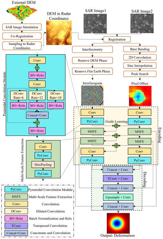
Figure 1.
The Overall structure of the proposed method.
To enhance reproducibility, we provide detailed specifications of the proposed JOTGLNet architecture. Table 1 summarizes the configuration of each layer, including the number of filters, kernel size, stride, and activation function. Unless otherwise specified, all convolutional layers use padding = same, bias = True, batch normalization (BN), and ReLU activation. The output layer adopts a linear activation to produce continuous deformation values.

Table 1.
Network architecture details (filters, kernel, stride, padding, activation).
2.1. Preliminary Deformation Inversion
2.1.1. Interferometry
Phase information is more delicate and accurate, but it is easily influenced by decoherence, which is the inconsistency of the ground scatterers in two SAR images. The inconsistency could be induced by large deformation, vegetation, precipitation, or other factors.
Interferometric phase measurement (InSAR) obtains phase information including phases from deformation , atmosphere , orbit error , the error phase caused by terrain errors and the difference between strong scatterers and pixel centers , and the noise phase [25]:
where represents the interferometric phase, which is the wrapped phase difference between the master and slave SLC images, and is the wrapping operator. The wrapped phase means the phase value is not an absolute value but a relative value, and the deformation must be retrieved according to the phase difference between adjacent pixels. In this situation, it is assumed that the real difference between two adjacent pixels is under half a cycle of the wavelength. Given both the fact that the signal travels around trip and the coherence of the wavelength, the phase difference usually should not exceed 1/4 of the wavelength. This assumption could be easily broken, and then made the phase unwrapping would fail.
2.1.2. Pixel Offset Tracking
Pixel offset tracking is a deformation retrieval method generally based on the amplitude information of SAR images [26]. It is unlikely to be influenced by the decoherence caused by large deformation and thus can retrieve deformation at the level of one meter or more [27]. These features make it a great addition to InSAR. By cross-correlation calculation, the very small pixel offset caused by deformation between two images can be determined and then used for the deformation inverse [28]. The accuracy of the offset tracking method is usually considered as 1/30–1/10 pixel size [29].
The offset tracking technology performs cross-correlation operations on the main and secondary image matching windows to find the pixel offset caused by the deformation, and combines the pixel size to obtain the deformation size. Current offset tracking technology based on SAR data mainly utilizes coherence, intensity, and phase information. Our purpose in this experiment was to use OT to obtain large gradient deformation and compensate for the decoherent areas in the phase image. The phase information in these areas is damaged, so we only use intensity information. Offset tracking mainly includes four steps: base banding, two-dimensional convolution, interpolation, and peak search. With the help of the Fourier transform, the convolution operation can be changed into a multiplication operation to improve the operation efficiency. The cross-correlation operation for this experiment is as follows:
where m and s are the matching windows of the main and secondary images, stands for Fourier transform, and is the inverse Fourier transform, and the symbol “·” indicates element-wise multiplication in the frequency domain, and the superscript “*” denotes the complex conjugate. If there is no offset, the cross-correlation peak should be in the center. Here we use and to represent the offset distance from the CC peak to the center in the slant-range and azimuth direction. If it is assumed that the deformation is only vertical, then it is proportional to . Then, an offset map that is proportional to the deformation can be expressed as . After obtaining the interference map and offset map containing deformation information, we performed model training.
2.2. Neural Network Structure
Neural-network-based phase unwrapping methods rely solely on phase information and often lack auxiliary inputs, such as stripe projection profiler, digital holographic interferometry, and magnetic resonance imaging (MRI). As a result, current deep-learning-based phase unwrapping models are mostly single-channel models. As previously stated, one of the challenges in the phase unwrapping for surface deformation is that excessive deformation can cause phase aliasing. This aliasing phenomenon is caused by the high speed of ground deformation during the acquisition time of the two SAR complex data. On the other hand, OT can accurately describe the geometric relation information in large-scale deformation regions, so it can be used as an important form of information compensation for large-scale ground deformation in the phase unwrapping methods. Therefore, the construction strategy of a multi-scale two-path neural network and the accurate loss function were redesigned in this study.
2.2.1. Construction of the Neural Network Structure
After the calculation in Section 2.1, the interferometric phase map and the pixel offset map can be represented as and , and the ground subsidence map can be estimated by
where is the relationship function of and constructed by the neural network to predict the ground subsidence map . In the interferogram inference channel of , suppose that is the inference process for the n-th layer and is the input of the n-th layer. In the OT-inference-channel of , is the inference process of the n-th layer, and is the input of the n-th layer. As previously analyzed, the interferometric phase map is more important than is the pixel offset map , but performs better than does in regions with rapid ground deformation. Therefore, the ground information mined by is regarded as an important form of compensation to provide reference for the interferogram inference channel as follows:
where ⊕ is the addition operation of feature maps obtained by the two channels, and the added feature maps are used for the input in the n-th layer of the interferogram inference channel to update . Therefore, is regarded as the corrected result obtained by and .
Considering the difference in the spatial size of different ground deformation regions, we constructed a pyramidal convolution module (PyConv) with dilated convolution operation to increase the receptive field of convolution operation so as to effectively extract features of different scales. In this work, the expansion rate of the dilated convolution operation is set to 6, 12, and 18, and the feature maps from the dilated convolution operation are added to the feature maps from the previous convolution layer so as to retain all the valid information as much as possible. At the same time, the pyramidal convolution modules of different layers are connected by the maximum pooling operation to constitute the multi-scale feature extraction (MSFE) process. After the operation process, the encoding process of the dual-channel neural network can be constructed, and the important features are saved in the output of the last PyConv operation, as shown in Figure 1.
In the decoding process, the feature maps from the dual-channel structure are implemented to deduce the settlement diagram M. The transposed convolution and upsampling are developed to restore the image size, and their function is opposite to the effect of max pooling. As the feature maps will lose some information after max pooling, the feature maps obtained from MSFE (before max pooling) in encoding are regarded as important information supplements and linked to the decoding features. After the inferring settlement diagram process is completed in different sizes, the predicted settlement diagram can be obtained.
2.2.2. Design of Loss Function
Further, to accurately capture the spatial texture relationship between the ground settlement map and interference fringes, a loss function based on shape sensing guidance was designed for the neural network to capture this spatial texture relationship accurately [30]. Reflected in the loss calculation, a morphological similarity measurement method was introduced to calculate the similarity between the generated ground settlement map and the real ground settlement map. Therefore, the average error information, such as MSE, can only be used to balance the average numerical error between the generated map and the real map, and the morphological similarity serves to correct the average error information so as to ensure the numerical balance between the region with large settlement change and the region with small settlement change in the settlement map in loss calculation.
In this study, the loss function was designed with two components: the similarity perception coefficient and the error measurement . These are calculated as follows:
where measures the similarity between the predicted settlement map and the actual settlement map. To avoid numerical instability when approaches zero or takes negative values, a small positive constant is added to the denominator, ensuring it is strictly positive and bounded above by slightly more than 1. A denominator close to 1 indicates a strong similarity between and M, while a denominator close to 0 indicates weak similarity. The similarity perception coefficient is computed using the Pearson correlation coefficient:
where represents the covariance calculation function, and represents the variance calculation function. The correlation coefficient quantifies the degree of linear correlation between and M, i.e., the morphological similarity.
In distance similarity measurement, the prior regularization term training rules of Elastic Net [31] are were referred to the in the design of distance loss, calculated as follows:
where is the mean square error (MSE) and is calculated by
where N is the number of pixels in the image, and is the coordinate in the image. is the mean absolute error and is calculated by
where is the equilibrium coefficient and is used to balance the metric relationship between and . In the experiments of this study, was set to 0.5.
2.3. Training Sample Generation
Although satellite SAR images are widely available, it is difficult to obtain sufficient real deformation data with reliable ground truth (e.g., GNSS or leveling) for training. Therefore, simulated deformation samples were generated based on a limited amount of real data in this study. The training sample generation strategy is presented in Figure 2. Moreover, validation using real InSAR data is outline in Section 3.5 to demonstrate the effectiveness of the proposed method.
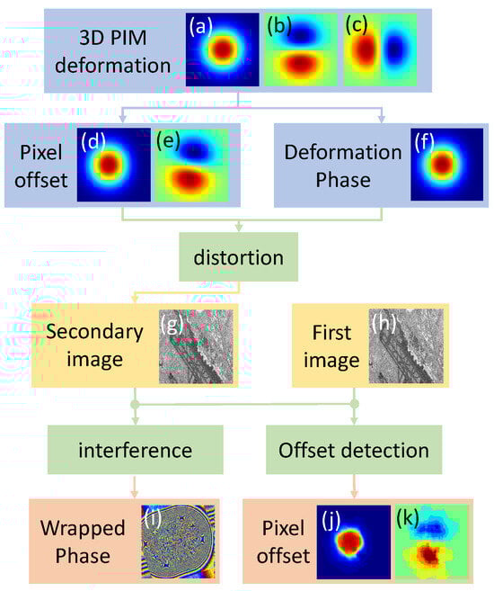
Figure 2.
Training sample generation: (a–c) are simulated deformation in the vertical, north–south, and west–east directions, respectively. (d,e) are the pixel offset caused by 3D deformation in the range and LOS directions, respectively. (f) is the deformation phase in the LOS direction. (g) is the slave image with the deformation caused by pixel offset and phase. (h) is the master image without deformation. (i) is the interferogram from (g,h). (j,k) are the pixel offsets between the master and slave images detected by offset tracking technology, respectively.
2.3.1. Three Kinds of Deformation
In generating realistic training samples, it is necessary to consider different stages of mining subsidence, which influence the shape and scale of surface deformation. With the mining activity continuing, the deformation on the ground surface expands towards the mining direction, the area becomes larger, and the maximum subsidence value increases; this phase is called “subcritical deformation”. When the mining distance underground reaches a threshold, the maximum subsidence value stops increasing and becomes a constant value, while the deformation area keeps increasing. The phase at this point is called “critical deformation”. After this phase, the deformation has a flat bottom because the maximum value no longer increases, and this phase is called “supercritical deformation”. The two important directions for the description of mining are the one towards the mining direction, called “strike direction”, and the one perpendicular to it, called “dip direction”. Based on the different phases, the mining deformation can be divided into three kinds, which are generated randomly:
- The deformation has not reached the maximum value. This happens with small mining activities or at the beginning of mining. At this moment the deformation shape can be described with a Gaussian surface [8].
- The deformation reaches the maximum value in only one of the two important directions. This happens under a long and narrow mining condition. In this situation, the deformation is no longer a standard Gaussian surface, but a stretched Gaussian surface with a line at its bottom.
- The deformation reaches the maximum value in two directions. This happens with a mining working face with enough width and length. In this situation, the deformation is a stretched Gaussian surface with a flat bottom.
2.3.2. Three-Dimensional Deformation Projection
Once vertical and horizontal deformations are generated, they can be projected into the SAR imaging geometry, including line-of-sight (LOS) and azimuth directions, to simulate actual SAR observations. After the generation of vertical subsidence, horizontal deformation should be generated as well. The horizontal movement is proportional to the first derivative of the subsidence value in the strike direction and dip direction [32]. The ratio of the maximum horizontal movement to the maximum subsidence value is called the horizontal movement coefficient [33], which is related to the mining depth, the width of the mining working face, and the inclination of the coal seam. A random number within the range of [0.2, 0.5] is used as the horizontal movement coefficient.
With 3D deformation, the projection of deformation in line of sight (LOS) (also known as slant range) and the azimuth direction of SAR geometry can be calculated as follows [34]:
where is the deformation projection in the LOS direction; are the vertical, west–east and north–south components of the real deformation vector, respectively; stands for the incidence angle of the resolution cell; and denotes the flight angles of the selected SAR sensor.
where is the deformation projection in the azimuth direction.
2.3.3. Deformation Integration
Deformation induces both phase differences and pixel offsets between master and slave SLC images. In this study, a specific training sample generation strategy was applied (Figure 2): we generate the deformation phase and pixel offset, and then add them to the slave image. Two advantages are considered. First, for high-resolution SAR images or strong deformation (beyond 1/10 pixel size), the pixel offset must be considered [35]. Second, the noise and atmosphere phases are already contained in the real SLC images, and they are more real than are the simulated ones. It is unrealistic to include all kinds of SAR images, which means the training result is not a general case. However, it is reasonable to assume that with the inclusion of pixel offset and more real noise and atmospheric phases, along with DEM and flat earth error phases, the result will be better in the training areas and with the same kinds of SLC images. The relationship between the deformation and pixel offset can be expressed as follows:
and
where and are the pixel offset in the slant range and azimuth direction, respectively; and and are the image resolution in the slant range and azimuth direction, respectively.
The deformation phase can be retrieved by the following:
where is the deformation phase, and is the wavelength of the radar sensor.
3. Experiments
3.1. Study Area and Dataset
In this study, four kinds of SLC images were applied as the training materials. They are detailed in Table 2. The 1-arcsecond (30 m) spacing Shuttle Radar Topography Mission (SRTM) Digital Elevation Model (DEM) is used to remove the topographic phase contributions [36].
Table 2.
Sensor and Image Characteristics.
A total of 20 TerraSAR-X SLC images with 4401 × 7601 (azimuth × range) pixels covering the Daliuta mining area in China were applied as the training materials, with a heading direction of , a wavelength of 3.11 cm, a spacing between samples of 0.85 m × 0.91 m in the azimuth and range, a resolution of 1.10 m × 1.17 m in the azimuth and range, and an incidence angle range from to . The study area was located in the Daliuta mining area in China. As shown in Figure 3, the optical image is TCI from Sentinel-2A, with the date being 21 August 2023 and the resolution being 10 m. There were 20 TerraSAR-X SLC images used to verify the proposed method, as shown in Figure 4.
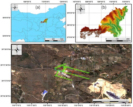
Figure 3.
Location and topography of the Daliuta area. The colored area in figure (a) shows the geographical location of the study area. Figure (b) shows the processed region of interest of the SAR image coverage. The green rectangle in figure (c) indicates the location of the working panel, while the red circles represent the locations of the GNSS stations.
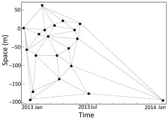
Figure 4.
Interferogram Selection.
Real-Time Kinematic(RTK) GNSS measurements were applied as the ground truth. 20130830 was used to verify the result on 20130710 because the surface was stable then, and the deformation did not change too much. Based on this actual scenario, we utilized the ground subsidence simulation methods outlined in Section 2.3.1 to create 5100 simulated samples, which were then randomly divided into training and test sets to evaluate the model. Detailed information is presented in Section 3.2.
3.2. Comparative Methods
To evaluate the effectiveness of the proposed method, six representative unwrapping approaches were selected for comparison, including two traditional path-following methods, one InSAR-OT fusion method, and three neural = network-based methods. The details are as follows:
3.2.1. Traditional Path-Following Methods
- MCF (Minimum Cost Flow): These methods address phase unwrapping as a network flow problem, finding the minimum-cost flow under constraints of phase continuity and smoothness. Variants improve efficiency or weight paths according to amplitude, closure error, or coherence [37].
- MST (Minimum Spanning Tree): These models formulate unwrapping as a minimum spanning tree problem that connects all nodes in a graph with minimal total edge weight [37].
3.2.2. Fusion Method (InSAR + OT)
- Coh.: This coherence-based InSAR-OT fusion method combines phase and OT results according to a coherence threshold [15,20]. Coherence measures the quality of interferograms; if it is below the threshold, the OT result is used; otherwise, the InSAR result is applied. In previous studies, the threshold was set to 0.5 and 0.3; in this study, we used an average value of 0.4. The coherence was estimated with a window using the method in [38]:
3.2.3. Neural Network Methods
- PUNet: This method treats phase unwrapping as a dense classification problem, predicting the wrap count at each pixel using a U-Net structure. Synthetic data with arbitrary shapes and Gaussian noise are used for training [8].
- PhaseNet 2.0: PhaseNet 2.0 is a similar solution to PUNet, only with a different network and loss function; that is, a fully convolutional DenseNet-based neural network and a new loss function that integrates residues and L1 loss [7].
- UNet: In this method, the phase unwrapping is transferred into a multiclass classification problem, and the convolutional segmentation network, i.e., UNet, is introduced to identify classes [14].
For deep learning experiments, the batch size was set to 8 and training epochs to 500, implemented in TensorFlow/Keras on an RTX 6000 GPU (NVIDIA Corporation, Santa Clara, CA, USA). A total of 5100 simulated settlement images were randomly divided into 4000 training samples and 1100 test samples. To avoid potential data leakage, the partitioning was performed strictly without overlap, ensuring that all test samples were entirely unseen during training. In PNet and UNet, the classification step was omitted for regions with fast settlement, while other network structures and parameters strictly followed the original implementations.
3.3. Ablation Experiment Results
A set of ablation experiments were designed to prove the rationality of the network structure, as shown in Table 3, and the root mean square error (RMSE) was used to evaluate the prediction accuracy of the ground subsidence.
Table 3.
The prediction results from the ablation experiments. “✓” indicates that the corresponding component was used in the ablation experiments.
In Exp. 3, 4, and 5, the effectiveness of the distance similarity loss and morphological similarity loss was proven. is the most common loss function in the regression models, and it was implemented in the five experiments. When there was only in the loss function, was set to 1. With the addition of distance similarity and the morphological similarity , the predicted error of RMSE can be reduced by around 0.03 and 0.05 respectively. Finally, the neural network structure of Exp. 5 was implemented in this study.
3.4. Comparative Experiment Results
3.4.1. Predicted Results
In the experiments, 1100 test samples with maximum ground deformation values ranging from 0 m to 12.6 m (absolute settlement values, i.e., negative vertical displacements) were analyzed. To evaluate the reasoning performance of different methods under various subsidence magnitudes, the samples were uniformly divided into 21 groups. The grouping criterion was based on a deformation interval of 0.6 m, so that the deformation range of each group did not exceed 0.6 m. The distribution of the 1100 test samples with respect to their maximum settlement is illustrated in Figure 5, which provides an overview of the deformation scales covered by the dataset. For each group, the predicted results are summarized in Table 4.
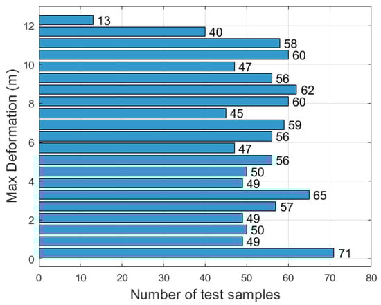
Figure 5.
Distribution of the 1100 test samples according to their maximum ground settlement values. The deformation magnitudes range from 0 m to 12.6 m and are uniformly divided into 21 groups with an interval of 0.6 m.
Table 4.
Prediction results from the different methods.
The predicted error of the whole image was recorded as , while the error restricted to the areas where deformation exceeded 10% of the maximum settlement was recorded as in order to reduce the interference of non-deforming regions in the accuracy evaluation. Based on and in each group, the average error (AvE) was calculated to demonstrate the stability of different methods across varying deformation scales. Additionally, the overall error (OaE) over all 1100 test samples was employed to assess the overall predictive performance of the methods. The results of and for the seven compared methods are presented in Figure 6 and Figure 7, respectively, and the detailed results are listed in Table 4.
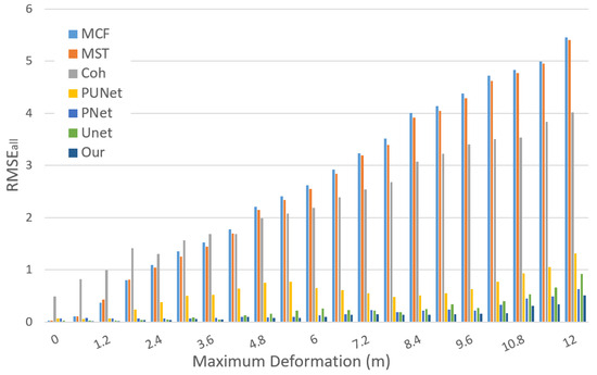
Figure 6.
of the seven methods.
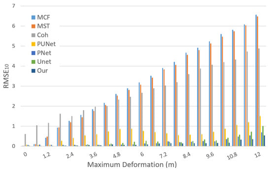
Figure 7.
of the seven methods.
It can be seen from Figure 6 and Figure 7 that for the traditional phase unwrapping methods, MCF and MST, with the increase of the maximum deformation, the RMSE increases as well. The conventional phase unwrapping methods work with the phase continuity assumption. When the deformation becomes larger, the phase gradient increases and the phases are more likely to be discontinuous, which leads to the unwrapping failure. The difference between MCF and MST is not obvious. For CIOF, the OT and InSAR are combined according to the coherence. OT has lower accuracy when the deformation is small [39]. For the situations of the maximum deformation below 1.8 m, OT introduces errors, and when the maximum deformationexceeds about 1.8 m, the advantage of OT is revealed. This phenomenon indicates that the fusion of InSAR and OT can improve large deformation monitoring, but it should be done in a more sophisticated way to avoid OT error in the small deformation areas. Compared with the three traditional methods, the network-based methods provided an obvious improvement. This is because network methods can learn to deduce the phase jump according to the surrounding textures. This characteristic can avoid the error that comes from the phase continuity assumption. PUNet had the largest RMSE compared with the other three network-based methods. Generally, the network is more powerful with a higher number of parameters [40]. PUNet has a minimal number of parameters in the four networks, so it is reasonable that it has the worst performance. Compared with the three reference network-based methods, the proposed method has the same magnitude of parameter number with PUNet and the lowest RMSE. The unique guided learning strategy and the large deformation information provided by OT reduce the learning costs of the network.
3.4.2. Visualized Analysis of Prediction Results with One Large/Small Deformation Sample
The objective of this section is to delve deeper into the predictive performance of diverse models. To achieve this, we will showcase the predictive results of various models under varying conditions of ground deformation. This visual comparison will highlight the disparities in performance among the different methods when predicting ground deformations. The comparative methods include traditional path-following approaches, exemplified by MCF and MST, neural network methodologies represented by PUNet and PNet, as well as the innovative method introduced in this paper, JOTGLNet. Recognizing the distinct sensitivity of these methods to ground deformation, we undertook an analysis of the results from two perspectives: large deformation (Figure 8) and small deformation (Figure 9).
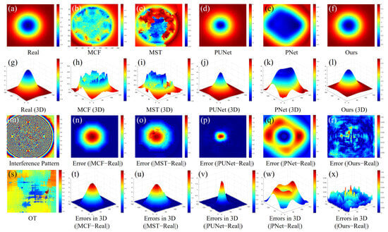
Figure 8.
Comparison of large ground deformation errors between the different methods: (a–f) are the ground deformation images; (g–l) are the ground deformation images in 3D; (m) is the interference image; (n–r) are the predicted errors; (s) is the OT map; (t–x) are the predicted errors in 3D.
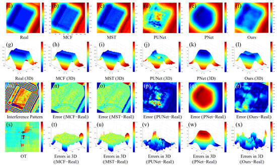
Figure 9.
Comparison of small ground deformation errors between the different methods: (a–f) are the ground deformation images; (g–l) are the ground deformation images in 3D; (m) is the interference image; (n–r) are the predicted errors; (s) is the OT map; (t–x) are the predicted errors in 3D.
In the figures, Figure 8a and Figure 9a are the simulated ground deformation images based on actual scenarios (labeled as “Real”), while their three-dimensional structures are represented in Figure 8g and Figure 9g. Correspondingly, Figure 8b–f and Figure 9b–f are the predicted results in 2D maps, and Figure 8b–f and Figure 9b–f are the predicted results in 3D maps. Their corresponding phase interferograms are presented in Figure 8m and Figure 9m, while the OT maps are shown in Figure 8s and Figure 9s. To provide a more detailed insight into the predictive capabilities of the different methods, we conducted a comparison between the predicted results (i.e., Figure 8b–f and Figure 9b–f) and the actual simulation outcomes (i.e., Figure 8a and Figure 9a). The corresponding errors are illustrated in Figure 8n–r and Figure 9n–r, while Figure 8t–x and Figure 9t–x present the three-dimensional structures of these errors.
In the large ground subsidence area, as shown in the interference fringes of Figure 8m, we can observe that in the central subsidence region, due to the accelerated subsidence speed, the interference fringes overlap, while the OT map (Figure 8s) provides more detailed information in these areas. From the prediction results, it is evident that the geodetic subsidence maps obtained by traditional methods (MCF (Figure 8b) and MST (Figure 8c)) differs significantly from the simulated scenario (Figure 8a), whereas the subsidence geodetic map derived from PUNet exhibits a smaller morphological error compared to the simulated subsidence scenario, albeit still showing some disadvantages compared to the model proposed in this study. This is reflected in the error maps: from a comparison of the errors from Figure 8n–r, it can be seen that PUNet (Figure 8p) demonstrates better prediction results, resulting in smaller errors, but still exhibits relatively large errors in the central region. In contrast, the errors obtained by our model eliminate the impact of rapid subsidence in the central deformation area (Figure 8r), thus achieving a more balanced error performance.
In the small ground subsidence area, as can be observed from the interference fringes in Figure 9m, the fringes did not overlap and their contours were relatively clear, thereby providing sufficient information for geodetic subsidence. Therefore, as evident from the prediction results of different models, traditional methods can also achieve good prediction performance (MCF (Figure 9b) and MST (Figure 9c)), while deep learning models do not demonstrate an advantage in this scenario (PUNet (Figure 9d) and MST (Figure 9e)), yielding significantly inferior results compared to traditional methods. The comparison becomes even clearer in the three-dimensional maps, i.e., Figure 9h–l. This observation aligns with the statistical results presented in Table 4. As can be seen from the error maps, the traditional methods (MCF (Figure 9n) and MST (Figure 9o)) can also achieve lower errors, whereas deep learning methods (PUNet (Figure 9p) and PNet (Figure 9q)) still exhibit substantial errors in the central subsidence region. In contrast, our model (Figure 9r) achieves better inference results with a more balanced error distribution.
In summary, neural network methods excel in predicting large-scale ground deformations, while the traditional methods slightly edge out in small deformation scenarios. However, our proposed method stands out for its superior accuracy and broader range of applicability, making it effective for both large and small deformation predictions.
3.5. Test Results in Daliuta
To further assess the practical effectiveness of the proposed method, we use real SAR images and GNSS-measured subsidence points, where the predicted subsidence curves are compared with those obtained by several baseline unwrapping approaches.
3.5.1. Data Description
The study area is located in Daliuta Town, China, a typical coal production region characterized by a thick and shallow coal seam overlain by loose layers, which causes severe surface deformation exceeding 1 cm/day. The dataset used in this study included two primary sources: TerraSAR-X SLC imagery and RTK GNSS measurements. A total of five spotlight TerraSAR-X images were acquired between 10 November 2012, and 5 May 2013, with a spatial resolution of 0.91 m in range and 0.86 m in azimuth [28]. Based on acquisition dates, these data were divided into five experimental sets (Data1–Data5), corresponding to 20121110–20121121, 20121110–20121202, 20121110–20121213, 20121110–20130402, and 20121110–20130505.
From the TerraSAR-X imagery, two types of data were generated following the procedure described in Section 2.3.1: (1) phase interferometry data, which serve as the primary input for most neural-network–based deformation prediction methods; and (2) pixel offset tracking (OT) data, which are combined with phase data in the proposed method to generate more reliable subsidence results. In addition, RTK GNSS measurements obtained at 70 observation points provided independent ground-truth subsidence values for the five experimental periods, which were used to validate the prediction results. The joint use of these datasets enabled a comprehensive evaluation of the proposed method under real deformation monitoring conditions.
3.5.2. Analysis of the Predicted Subsidence Curve
The prediction procedure was conducted as follows: using models trained with the neural network methods described in Section 3.2, we input real interferograms and OT data from five time teams (Data 1–5) to generate the corresponding ground deformation maps. The resulting subsidence maps were sampled at 70 GNSS stations to obtain settlement curves for all five time periods, as visualized in Figure 10, which allowed for the comparison of the proposed method with baseline unwrapping approaches at representative GNSS points.

Figure 10.
Comparative analysis of settlement curves derived from various neural-network-based and traditional phase unwrapping methods against GNSS ground-truth measurements across five data sets. Subplots (a–e) correspond to Data 1–5, respectively. The horizontal axis represents the measurement point index, and the vertical axis indicates the deformation value (unit: meters). Subplot (f) provides the legend, where each line style/color corresponds to a specific method.
The GNSS measurements varied between 0 and −4 m, indicating significant ground subsidence. In regions with small deformation gradients (e.g., Figure 10a–c, between measurement points 40 and 50), the neural-network-based methods frequently deviated from the reference GNSS data, either underestimating or overestimating the actual subsidence, and these discrepancies were more pronounced where deformation changed abruptly.
By contrast, the three conventional phase unwrapping methods (MCF, MST, and Coh.) predicted values fluctuating only within −0.5 to 0.5 m, substantially underestimating the true deformation magnitude and showing low correlation with the GNSS curves. This indicates that traditional approaches suffer from systematic bias in regions with large deformation gradients and are unable to capture the full range of subsidence.
In regions with relatively large deformation (e.g., Figure 10d,e, points 20–40 and 50–60), all neural-network-based methods reproduced the overall trend, but the proposed approach demonstrated superior consistency and smoother alignment with GNSS measurements, reducing high-frequency fluctuations and better capturing the magnitude and spatial trend of deformation.
Overall, these results underscore that the integration of phase interferometry with OT data significantly enhances prediction reliability and accuracy, especially in challenging scenarios involving complex or rapid subsidence patterns.
3.5.3. Evaluation of Prediction Performance
Table 5 presents a quantitative comparison among three traditional methods (MCF, MST, and Coh.) and four neural-network-based methods (PNet, PUNet, UNet, and Ours) across five datasets. Among the traditional approaches, Coh. consistently outperformed MCF and MST in most metrics due to its improved phase unwrapping strategy, which mitigates error accumulation in regions with abrupt or complex subsidence. In contrast, MCF and MST often exhibited large errors in high-deformation regions, with an RMSE up to 2.4323 m and an MAE up to 1.9229 m (Data5), which reflects limited adaptability to rapid subsidence. Models based on neural network methods demonstrated substantial improvements over conventional methods across all datasets. In large deformation gradient regions such as Data3, UNet and our method achieved the lowest RMSE (0.2118–0.2536 m) and MAE (0.0942–0.1034 m), indicating that learning-based approaches can accurately capture both the magnitude and spatial trend of rapid subsidence.
Table 5.
Performance comparison of seven models (MCF, MST, Coh, PNet, PUNet, UNet, and Ours) across five datasets (Data1–Data5) and the average (Avg.) for RMSE, MAE, Bias, CC, and MAPE. The best values in each row are highlighted in bold.
Moreover, the correlation coefficients (CC) of traditional methods were often low or even negative in some datasets (e.g., MCF: 0.3949 in Data1, −0.0796 in Data5), which reflects a weak correlation with true deformation under conditions of low interferometric coherence. In contrast, our model consistently maintained high CC values (>0.97) across all datasets, demonstrating strong generalization and robust accuracy even when coherence varied. In addition, the bias results further confirmed the reliability of the proposed model, as it achieved the lowest average bias (0.0697 m), indicating that the predictions are not only accurate in magnitude but also free from significant systematic overestimation or underestimation. It is worth noting that the extremely high MAPE values reported in some cases (e.g., Data2 and Data3) were mainly caused by GNSS measurements with deformation values close to zero, which resulted in near-zero denominators in the MAPE calculation. This issue is not reflective of the actual prediction performance but rather a limitation of the metric itself under such conditions. Nevertheless, in regions with moderate-to-large deformation magnitudes, the MAPE values remained reasonable and further support the superior accuracy of the proposed method compared with other approaches.
These quantitative results align well with the qualitative observations in Figure 10. For instance, in Figure 10c (Data3), which corresponds to large deformation gradients (points 40–50), UNet and our method achieve the two lowest RMSE and MAE values, consistent with the closer alignment of UNet’s and our method’s curves with the GNSS reference. In moderate-deformation regions such as Data1 and Data4 (Figure 10a,d), all methods performed reasonably well, yet our method still maintained the lowest or second-lowest amount of errors, corresponding to smooth and precise prediction curves. These observations confirm that the proposed model can accurately capture both rapid and moderate subsidence trends while reducing error accumulation in low-coherence or complex regions.
Overall, our method achieved the lowest average RMSE (0.2497 m), MAE (0.1439 m), bias (0.0697 m), and MAPE (82.036%), along with the highest average CC (0.9784). These results indicate superior accuracy and generalization compared with both conventional and other learning-based methods, particularly under conditions of rapid subsidence and varying interferometric coherence, where traditional methods often fail.
3.6. Efficiency and Parameter Analysis of Neural Networks
In addition to prediction performance, the number of model parameters is also a crucial indicator for evaluating model performance, especially in scenarios where computer resources are limited. Achieving superior inference capabilities with lightweight models is an important goal researchers strive for. The difference in the parameter setting in the neural network can directly affect the consumption of computer resources and the efficiency of model inference. To make the experimental results as close as possible to the original paper, the comparison neural networks in this study were set according to the number of parameters reported in the original papers. The memory size, number of parameters, and FLOPs of these neural networks are shown in Table 6. Compared with the approximately 29 million parameters of the PNet and UNet models, our proposed method only has 5 million parameters, occupies 58 MB of memory, and requires 117 GFLOPs for a single forward pass. The number of parameters is reduced to less than , while of OaE is reduced by more than ; i.e., the predicted error of is decreased by 28.6%. Compared with PUNet, the number of parameters of our method is increased by 1.3 times, while the predicted error of is decreased by 75%. To be fair, the number of filters in PUNet is increased from 64 to 128, resulting in 8.7 million parameters and 100.6 MB of memory. As a result, of AoE can reach 0.2, decreasing by 0.4, but it is still inferior to our method in terms of the prediction results. Although some networks have fewer FLOPs, the lightweight design of our method maintains fast inference speed and higher prediction accuracy, making it suitable for practical deformation monitoring.
Table 6.
The size of different neural networks.
4. Discussion
4.1. Complementary Roles of Interferometric Phase and Offset Tracking
The experimental results strongly validate the complementary nature of interferometric phase and pixel offset tracking (OT) that our dual-path network is designed to exploit. As evidenced in Table 4 and Figure 6 and Figure 7, traditional InSAR methods (MCF, MST) perform well for small deformations ( < 0.5 m for [0, 1.8 m]), but their accuracy degrades rapidly as the deformation gradient increases due to phase aliasing and coherence loss. Conversely, the coherence-based fusion method (Coh.) performs poorly in small deformation regimes (: 0.5–1.0 m for [0, 1.8 m]) because OT’s inherent accuracy is proportional to pixel resolution, which introduces noise where phase information is superior. However, its relative performance improves for large deformations (>1.8 m), highlighting OT’s strength.
Our JOTGLNet successfully leverages both sources: it matches or surpasses traditional methods in low-deformation scenarios (Figure 9, Table 4: = 0.01 m for [0, 0.6 m]) while dramatically outperforming all others in high-deformation regimes (Figure 8, Table 4: OaE = 0.15 m versus > 0.27 m for others). This is because the interferometric branch provides high-precision data in coherent areas, while the OT branch acts as a reliable guide in high-gradient regions where fringes are aliased (Figure 8m versus s), preventing the network from making large errors in the subsidence center. The quantitative results in Table 5 on real data further confirm this, showing that our method maintains high accuracy (low RMSE/MAE) and consistency (high CC) across all five datasets with varying deformation magnitudes.
4.2. Deformation Gradients and Geohazard Interpretation
While maximum deformation values are a key output, the spatial gradients of deformation are often more critical for risk assessment. Our method’s ability to accurately capture these gradients is demonstrated not just in the predicted deformation maps (Figure 8f and Figure 9f) but, more importantly, in the spatial distribution of prediction errors (Figure 8n–r and Figure 9n–r). Traditional methods and other deep learning models showed concentrated and significant errors in the high-gradient zones surrounding the subsidence center. In contrast, the error distribution of our method was more balanced and minimal across the entire deformation region. This indicates superior capture of the entire deformation morphology, not just the peak value. This capability is crucial for practical applications, as sharp gradients often indicate potential zones of tension cracking or structural instability, and accurately mapping these zones is essential for preventative hazard mitigation.
4.3. Role of Shape Perception Loss in Regional Adaptability
The designed shape perception loss function is a key contributor to the model’s performance, a fact directly supported by the ablation study results in Table 3 (Exps. 3–5). Using only MSE loss (Exp. 3) yielded an RMSE of 0.2278. Incorporating the MAE term to balance distance similarity (Exp. 4) reduced the error to 0.1984. The full loss function, which integrates the morphological similarity coefficient (Exp. 5), further reduced the RMSE to 0.1496. This progressive improvement proves that guiding the network to learn the geometric structure and spatial correlation of deformation (via ), in addition to pixel-wise distance, is more effective than is relying on distance metrics solely. This loss design directly addresses the issue of unbalanced deformation within samples, forcing the network to learn from the periphery towards the center, which is reflected in the more homogeneous error maps (Figure 8r and Figure 9r).
4.4. Practicality of Synthetic Sample Generation
The use of synthetically generated training samples is justified by the model’s successful application to the real, unseen TerraSAR-X data, as described in Section 3.5. The high performance on the Daliuta datasets (Table 5, Figure 10), which contain natural noise, atmospheric artifacts, and real decorrelation patterns absent from simulated data, demonstrates the strong generalization ability learned by the model. This is because our generation strategy embeds realistic deformation signals into actual SLC images, thus preserving the complex statistical properties and error sources of real SAR data. This approach provides a scalable and practical solution for training data-intensive deep learning models in a domain where fully annotated real-world ground truth is extremely rare and difficult to obtain.
4.5. Potential Extensions to Complex Geological Hazards
Although this study focused on mining-induced subsidence, the framework has potential for monitoring broader geohazards. Earthquakes, volcanic uplift, and landslides produce complex deformation signatures that challenge conventional InSAR or OT methods when used alone. The dual-path architecture, combined with shape perception loss, may detect both subtle pre-event deformation and abrupt post-event displacement. Future research could integrate temporal coherence constraints, multi-sensor fusion, or domain-adapted network modules to further enhance detection capabilities. This demonstrates the broader applicability and value of the method for disaster prevention, urban safety, and ecological protection.
5. Conclusions
To enable the model to learn more comprehensive information about ground deformation, this paper proposes a guided learning network with joint offset tracking for multiscale deformation monitoring. In this network, interferograms are used as the primary information source, while pixel offset tracking is incorporated as auxiliary information to achieve multi-information interaction. Additionally, a shape perception loss function is designed to refine the error representation, enabling the model to better capture spatial patterns and morphological consistency across regions with varying subsidence rates. Due to the difficulty in obtaining sufficiently diverse and well-labeled ground deformation data, we developed a training sample generation strategy using TerraSAR-X SLC images from the Daliuta mining area. By introducing three distinct deformation phases and corresponding pixel offsets into slave SLC images, we simulated mining-induced ground subsidence and constructed interferograms and OT maps as network inputs. Based on these data, extensive experiments were conducted, and the results demonstrated the validity and effectiveness of the proposed approach. To further ensure the reliability of evaluation, five TerraSAR-X experimental datasets (Data1–Data5) together with 70 RTK GNSS observation points were employed as an independent benchmark to assess real-world performance, where JOTGLNet consistently achieved good precision and superior robustness compared with state-of-the-art methods.
Despite the promising results, several limitations of this study should be acknowledged. Firstly, the performance of JOTGLNet remains tied to the quality and characteristics of the training data. Although the proposed synthetic sample generation strategy effectively mimics real scenarios, its generalization capability to other geological settings or SAR sensors with distinct imaging parameters (e.g., Sentinel-1, Gaofen-3, different wavelengths or incidence angles) requires further validation and potential fine-tuning. Secondly, while JOTGLNet is relatively lightweight compared with existing deep networks (≈5.1M parameters, 58.7 MB, 117 GFLOPs per inference), computational efficiency is still a consideration for real-time and large-area monitoring applications, motivating future work on model pruning, quantization, and deployment optimization. Thirdly, in extremely low-coherence scenarios (e.g., dense vegetation or rapid temporal decorrelation), the robustness of the method, although enhanced by OT, remains limited. Future research will therefore explore the integration of multi-temporal SAR stacks and self-supervised or transfer learning strategies to reduce reliance on simulated training data, as well as the extension of the framework to broader geohazard applications such as mining subsidence early warning, landslides, earthquakes, and urban infrastructure monitoring. These efforts will guide future work toward more practical and operational deployment. In particular, JOTGLNet has the potential to support mining subsidence early warning systems and geological disaster monitoring platforms by providing accurate, near real-time deformation information, while future efforts will focus on improving cross-region generalization, reducing computational cost, and integrating multi-source SAR data for practical operational deployment.
Author Contributions
Conceptualization, methodology, and writing—original draft preparation, J.N.; validation, visualization, and writing—review and editing, S.B.; experiments and writing—original draft preparation, X.L.; software, validation, and writing—review and editing, S.D.; resources, formal analysis, and data curation, D.T.; investigation and writing—review and editing, Y.Z. All authors have read and agreed to the published version of the manuscript.
Funding
This work was supported by the Yunnan Provincial Major Science and Technology Special Plan Projects (202502AC080006), by the National Natural Science Foundation of China under Grant 62302429, by the Open Foundation of National Key Laboratory of Microwave Imaging Technology (AIRZB76-2023-000573), by the Deng Cheng Expert Workstation of Yunnan Province (202305AF150202), by the Spanish Agencia Estatal de Investigacion under Grant G2HOTSPOTS (PID2021-1221420B-100), and by the AEl, Ministerio de Ciencia, Innovación y Universidades. Convocatoria Proyectos en Colaboración Público Privada, 2021, under Grant CPP2021-009072(STONE).
Data Availability Statement
Data are contained within the article.
Conflicts of Interest
Author Yibing Zhan was employed by the company JD Explore Academy. The remaining authors declare that the research was conducted in the absence of any commercial or financial relationships that could be construed as a potential conflict of interest.
References
- Li, S.; Xu, W.; Li, Z. Review of the SBAS InSAR Time-Series Algorithms, Applications, and Challenges. Geodesy Geodyn. 2022, 13, 114–126. [Google Scholar] [CrossRef]
- Nagler, T.; Libert, L.; Wuite, J.; Hetzenecker, M.; Keuris, L.; Rott, H. Comprehensive ICE Sheet Wide Velocity Mapping Combining SAR Interferometry and Offset Tracking. In Proceedings of the IGARSS 2022 IEEE International Geoscience and Remote Sensing Symposium, Kuala Lumpur, Malaysia, 17–22 July 2022; IEEE: Piscataway, NJ, USA, 2022; pp. 3888–3891. [Google Scholar] [CrossRef]
- Hooper, A.; Bekaert, D.; Spaans, K.; Arıkan, M. Recent Advances in SAR Interferometry Time Series Analysis for Measuring Crustal Deformation. Tectonophysics 2012, 514, 1–13. [Google Scholar] [CrossRef]
- Zhu, X.X.; Montazeri, S.; Ali, M.; Hua, Y.; Wang, Y.; Mou, L.; Shi, Y.; Xu, F.; Bamler, R. Deep Learning Meets SAR: Concepts, Models, Pitfalls, and Perspectives. IEEE Geosci. Remote Sens. Mag. 2021, 9, 143–172. [Google Scholar] [CrossRef]
- Zhong, H.; Tang, J.; Zhang, S. Phase Quality Map Based on Local Multi-Unwrapped Results for Two-Dimensional Phase Unwrapping. Appl. Opt. 2015, 54, 739–745. [Google Scholar] [CrossRef]
- Yin, Q.; Lin, Z.; Hu, W.; López-Martínez, C.; Ni, J.; Zhang, F. Crop Classification of Multitemporal PolSAR Based on 3-D Attention Module with ViT. IEEE Geosci. Remote Sens. Lett. 2023, 20, 1–5. [Google Scholar] [CrossRef]
- Spoorthi, G.E.; Gorthi, R.K.S.S.; Gorthi, S. PhaseNet 2.0: Phase Unwrapping of Noisy Data Based on Deep Learning Approach. IEEE Trans. Image Process. 2020, 29, 4862–4872. [Google Scholar] [CrossRef]
- Wu, Z.; Wang, T.; Wang, Y.; Wang, R.; Ge, D. Deep Learning for the Detection and Phase Unwrapping of Mining-Induced Deformation in Large-Scale Interferograms. IEEE Trans. Geosci. Remote Sens. 2021, 60, 1–18. [Google Scholar] [CrossRef]
- Yin, W.; Chen, Q.; Feng, S.; Tao, T.; Huang, L.; Trusiak, M.; Asundi, A.; Zuo, C. Temporal Phase Unwrapping Using Deep Learning. Sci. Rep. 2019, 9, 20175. [Google Scholar] [CrossRef] [PubMed]
- Zhao, J.; Liu, L.; Wang, T.; Wang, X.; Du, X.; Hao, R.; Liu, J.; Liu, Y.; Zhang, J. VDE-Net: A Two-Stage Deep Learning Method for Phase Unwrapping. Opt. Express 2022, 30, 39794–39815. [Google Scholar] [CrossRef]
- Murdaca, G.; Rucci, A.; Prati, C. Deep Learning for InSAR Phase Filtering: An Optimized Framework for Phase Unwrapping. Remote Sens. 2022, 14, 4956. [Google Scholar] [CrossRef]
- Zhu, S.; Zang, Z.; Wang, X.; Wang, Y.; Wang, X.; Liu, D. Phase Unwrapping in ICF Target Interferometric Measurement via Deep Learning. Appl. Opt. 2021, 60, 10–19. [Google Scholar] [CrossRef] [PubMed]
- Li, L.; Zhang, H.; Tang, Y.; Wang, C.; Gu, F. InSAR Phase Unwrapping by Deep Learning Based on Gradient Information Fusion. IEEE Geosci. Remote Sens. Lett. 2021, 19, 1–5. [Google Scholar] [CrossRef]
- Zhang, J.; Tian, X.; Shao, J.; Luo, H.; Liang, R. Phase Unwrapping in Optical Metrology via Denoised and Convolutional Segmentation Networks. Opt. Express 2019, 27, 14903–14912. [Google Scholar] [CrossRef]
- Ma, J.; Yang, J.; Zhu, Z.; Cao, H.; Li, S.; Du, X. Decision-Making Fusion of InSAR Technology and Offset Tracking to Study the Deformation of Large Gradients in Mining Areas—Xuemiaotan Mine as an Example. Front. Earth Sci. 2022, 10, 962362. [Google Scholar] [CrossRef]
- Chen, Y.; Bruzzone, L. Self-Supervised SAR-Optical Data Fusion and Land-Cover Mapping Using Sentinel-1/-2 Images. arXiv 2021, arXiv:2103.05543. [Google Scholar] [CrossRef]
- Wang, J.; Fan, X.; Zhang, Z.; Zhang, X.; Nie, W.; Qi, Y.; Zhang, N. Spatiotemporal Mechanism-Based Spacetimeformer Network for InSAR Deformation Prediction and Identification of Retrogressive Thaw Slumps in the Chumar River Basin. Remote Sens. 2024, 16, 1891. [Google Scholar] [CrossRef]
- Zhang, J.; Gao, J.; Gao, F. Time Series Land Subsidence Monitoring and Prediction Based on SBAS-InSAR and GeoTemporal Transformer Model. Earth Sci. Inform. 2024, 17, 5899–5911. [Google Scholar] [CrossRef]
- Strozzi, T.; Luckman, A.; Murray, T.; Wegmuller, U.; Werner, C.L. Glacier Motion Estimation Using SAR Offset-Tracking Procedures. IEEE Trans. Geosci. Remote Sens. 2002, 40, 2384–2391. [Google Scholar] [CrossRef]
- Chen, B.; Deng, K.; Fan, H.; Yu, Y. Combining SAR Interferometric Phase and Intensity Information for Monitoring of Large Gradient Deformation in Coal Mining Area. Eur. J. Remote Sens. 2015, 48, 701–717. [Google Scholar] [CrossRef]
- Johnson, J.; Alahi, A.; Fei-Fei, L. Perceptual Losses for Real-Time Style Transfer and Super-Resolution. In Proceedings of the European Conference on Computer Vision, Amsterdam, The Netherlands, 11–14 October 2016; Springer: Cham, Switzerland, 2016; pp. 694–711. [Google Scholar] [CrossRef]
- Cheng, G.; Han, J.; Lu, X. Remote Sensing Image Scene Classification: Benchmark and State of the Art. Proc. IEEE 2017, 105, 1865–1883. [Google Scholar] [CrossRef]
- Bamler, R.; Hartl, P. Synthetic Aperture Radar Interferometry. Inverse Probl. 1998, 14, R1–R54. [Google Scholar] [CrossRef]
- Hu, J.; Li, Z.; Ding, X.; Zhu, J.; Zhang, L.; Sun, Q. Pixel Offset Tracking for Large Scale Landslide Monitoring: Case Study of Baige Landslide. Remote Sens. 2014, 6, 11635–11652. [Google Scholar]
- Zheng, M.; Zhang, H.; Deng, K.; Du, S.; Wang, L. Analysis of Pre- and Post-Mine Closure Surface Deformations in Western Xuzhou Coalfield from 2006 to 2018. IEEE Access 2019, 7, 124158–124172. [Google Scholar] [CrossRef]
- Du, S.; Mallorqui, J.J.; Zhao, F. ACE-OT: Polarimetric SAR Data-Based Amplitude Contrast Enhancement Algorithm for Offset Tracking Applications. IEEE Trans. Geosci. Remote Sens. 2022, 60, 1–15. [Google Scholar] [CrossRef]
- Cai, J.; Zhang, L.; Dong, J.; Wang, C.; Liao, M. Polarimetric SAR Pixel Offset Tracking for Large-Gradient Landslide Displacement Mapping. Int. J. Appl. Earth Obs. Geoinf. 2022, 112, 102867. [Google Scholar] [CrossRef]
- Du, S.; Mallorqui, J.J.; Zhao, F. Patch-Like Reduction (PLR): A SAR Offset Tracking Amplitude Filter for Deformation Monitoring. Int. J. Appl. Earth Obs. Geoinf. 2022, 113, 102976. [Google Scholar] [CrossRef]
- Huang, J.; Bai, Y.; Lei, S.; Deng, K. Time-Series SBAS Pixel Offset Tracking Method for Monitoring Three-Dimensional Deformation in a Mining Area. IEEE Access 2020, 8, 118787–118798. [Google Scholar] [CrossRef]
- Ni, J.; Xiang, D.; Lin, Z.; López-Martínez, C.; Hu, W.; Zhang, F. DNN-Based PolSAR Image Classification on Noisy Labels. IEEE J. Sel. Top. Appl. Earth Obs. 2022, 15, 3697–3713. [Google Scholar] [CrossRef]
- Zou, H.; Hastie, T. Regularization and Variable Selection via the Elastic Net. J. R. Stat. Soc. B 2005, 67, 301–320. [Google Scholar] [CrossRef]
- Yang, Z.F.; Li, Z.W.; Zhu, J.J.; Hu, J.; Wang, Y.J.; Chen, G.L. InSAR-Based Model Parameter Estimation of Probability Integral Method and Its Application for Predicting Mining-Induced Horizontal and Vertical Displacements. IEEE Trans. Geosci. Remote Sens. 2016, 54, 4818–4832. [Google Scholar] [CrossRef]
- Fan, H.; Gao, X.; Yang, J.; Deng, K.; Yu, Y. Monitoring Mining Subsidence Using a Combination of Phase-Stacking and Offset-Tracking Methods. Remote Sens. 2015, 7, 9166–9183. [Google Scholar] [CrossRef]
- Fialko, Y.; Simons, M.; Agnew, D. The Complete (3-D) Surface Displacement Field in the Epicentral Area of the 1999 Mw7.1 Hector Mine Earthquake, California, from Space Geodetic Observations. Geophys. Res. Lett. 2001, 28, 3063–3066. [Google Scholar] [CrossRef]
- Ni, J.; Zhang, F.; Ma, F.; Yin, Q.; Xiang, D. Random Region Matting for the High-Resolution PolSAR Image Semantic Segmentation. IEEE J. Sel. Top. Appl. Earth Obs. 2021, 14, 3040–3051. [Google Scholar] [CrossRef]
- Farr, T.G.; Rosen, P.A.; Caro, E.; Crippen, R.; Duren, R.; Hensley, S.; Kobrick, M.; Paller, M.; Rodriguez, E.; Roth, L.; et al. The Shuttle Radar Topography Mission. Rev. Geophys. 2007, 45, RG2004. [Google Scholar] [CrossRef]
- Gens, R. Phase Unwrapping. In Proceedings of the GEOS 639 InSAR and Its Applications, Fairbanks, AK, USA, Fall 2006; University of Alaska Fairbanks: Fairbanks, AK, USA, 2006. [Google Scholar]
- Touzi, R.; Lopes, A.; Bruniquel, J.; Vachon, P.W. Coherence Estimation for SAR Imagery. IEEE Trans. Geosci. Remote Sens. 1999, 37, 135–149. [Google Scholar] [CrossRef]
- Amitrano, D.; Costantini, M.; Dell’Aglio, D.; Iodice, A.; Malvarosa, F.; Minati, F.; Riccio, D.; Ruello, G. Landslide Monitoring Using SAR Sub-Pixel Offset Tracking. In Proceedings of the 2018 IEEE 4th International Forum on Research and Technology for Society and Industry (RTSI), Palermo, Italy, 10–13 September 2018; IEEE: New York, NY, USA, 2018; pp. 1–4. [Google Scholar]
- Bergstra, J.; Bengio, Y. Random Search for Hyper-Parameter Optimization. J. Mach. Learn. Res. 2012, 13, 281–305. [Google Scholar]
Disclaimer/Publisher’s Note: The statements, opinions and data contained in all publications are solely those of the individual author(s) and contributor(s) and not of MDPI and/or the editor(s). MDPI and/or the editor(s) disclaim responsibility for any injury to people or property resulting from any ideas, methods, instructions or products referred to in the content. |
© 2025 by the authors. Licensee MDPI, Basel, Switzerland. This article is an open access article distributed under the terms and conditions of the Creative Commons Attribution (CC BY) license (https://creativecommons.org/licenses/by/4.0/).