Article

Unveiling Forest Density Dynamics in Saihanba Forest Farm by Integrating Airborne LiDAR and Landsat Satellites

State Key Laboratory of Remote Sensing and Digital Earth, Faculty of Geographical Science, Beijing Normal University, Beijing 100875, China
*
Author to whom correspondence should be addressed.
Remote Sens. 2025, 17(19), 3338; https://doi.org/10.3390/rs17193338
Submission received: 31 July 2025 / Revised: 23 September 2025 / Accepted: 28 September 2025 / Published: 29 September 2025
(This article belongs to the Special Issue Digital Modeling for Sustainable Forest Management)

Abstract

Highlights

What are the main findings?
  • Multi-seasonal inputs significantly outperformed single-season Landsat data in estimating tree density, exhibiting superior model accuracy and generalization.
What is the implication of the main finding?
  • Supports ecological evaluation of large-scale afforestation in Saihanba based on produced five-year interval tree density maps (1988–2023), demonstrating the utility of multi-source remote sensing for tracking forest recovery over time.

Abstract

Forest density is a key parameter in forestry research, and its variation can significantly impact ecosystems. Saihanba, as a focal site for afforestation and restoration, offers an ideal case for monitoring these dynamics. In this study, we compared three machine learning algorithms—Random Forest, Support Vector Regression, and XGBoost—using Landsat surface reflectance data together with the Normalized Difference Vegetation Index (NDVI) and the Enhanced Vegetation Index (EVI), and reference tree densities derived from LiDAR individual tree segmentation. The best-performing algorithm, XGBoost (R2 = 0.65, RMSE = 174 trees ha−1), was then applied to generate a long-term forest density dataset for Saihanba at five-year intervals, covering the period from 1988 to 2023. Results revealed distinct differences among tree species, with larch achieving the highest accuracy (R2 = 0.65, RMSE = 161 trees ha−1), whereas spruce had larger prediction errors (RMSE = 201 trees ha−1) despite a relatively high R2 (0.70). Incorporating 30 m slope data revealed that moderate slopes (5–30°) favored faster forest recovery. From 1988 to 2023, average forest density rose from 521 to 628 trees ha−1—a 20.6% increase—demonstrating the effectiveness of restoration and providing a transferable framework for large-scale ecological monitoring.

1. Introduction

As a key carbon sink in terrestrial ecosystems, forest ecosystems rely heavily on the accurate quantification of structural parameters to assess carbon storage dynamics [1]. Among these parameters, the number of trees per unit area is a fundamental indicator of forest density. It directly affects light-use efficiency and interspecies competition within forest stands and is also a crucial factor in determining the carbon sink capacity of forests [2].
Traditional ground plot surveys, while capable of providing highly accurate local data [3], are limited by high time costs and insufficient spatial coverage when applied to vast and complex forest terrains, making them unsuitable for large-scale and long-term monitoring [4]. As a result, leveraging remote sensing technologies to efficiently and accurately estimate forest density has become a major research focus in forest ecosystem monitoring and management [5].
Many researchers have used different remote sensing techniques to estimate tree density. A common approach involves acquiring high-resolution data from aerial platforms, such as Unmanned Aerial Vehicles (UAVs), to obtain high-resolution imagery or three-dimensional (3D) Light Detection and Ranging (LiDAR) point clouds for forest density extraction. High-resolution imagery allows for image segmentation and object counting through image processing techniques, thereby estimating forest density in the study area [6]. LiDAR data, on the other hand, provides 3D point clouds from which individual trees can be segmented to calculate tree density [7]. However, the high cost of acquiring such data limits their applicability for long-term, large-scale monitoring.
In contrast, satellite remote sensing offers a more cost-effective means of obtaining large-scale data. In particular, freely available satellite datasets provide great convenience for large-scale remote sensing monitoring. For example, Crowther et al. used global Moderate-resolution Imaging Spectroradiometer (MODIS) and other remote sensing data combined with field surveys to develop a generalized linear regression model for estimating global tree density [8]. Among medium- and high-resolution satellite datasets, the Sentinel-2 series has gained popularity in recent years due to its higher spatial resolution and a greater number of spectral bands. Zhang et al. explored the empirical relationship between vegetation cover and tree density using Sentinel-2 data [9], demonstrating the potential of medium-resolution satellite data for density estimation. However, since the study area covered only a few hectares (ha), the reference tree density could be obtained through visual interpretation, which limits the method’s applicability for larger-scale validation and extension. Furthermore, Sentinel-2 has only been available in recent years, lacking a long historical archive for time-series analysis.
Compared to Sentinel-2, the Landsat series offers a long-term observational archive that enables long-term density monitoring [10]. Its 30 m pixel size also roughly corresponds to the size of ground sampling plots, making it suitable for integration with field survey data. Studies using Landsat imagery have shown that results based on multi-temporal data outperform those using single-date imagery [11], providing useful insights for subsequent research [12].
Field measurements are crucial for inversion studies. Ground surveys and UAV-based remote sensing are both valuable for obtaining such reference data [13]. However, the reachability of ground areas and the payload limitations of UAVs often constrain the spatial extent of data collection [14]. In contrast, airborne LiDAR systems can rapidly collect large-scale ground point cloud data [15]. After individual tree segmentation, these data yield accurate, large-scale tree density values, serving as robust reference and validation datasets [16]. These structured, spatially explicit ground samples are not only essential for validating inversion models but are also well-suited for integration with remote sensing imagery in machine learning and modeling workflows.
In terms of inversion methods, while linear regression models are simple and computationally efficient—suitable for exploring linear relationships between remote sensing features and tree density [8,9,17]—the actual relationship is often nonlinear and multi-scale in nature [18]. To better capture these complex feature-response patterns, researchers have increasingly adopted machine learning algorithms such as Random Forest and Extreme Gradient Boosting (XGBoost) in recent years [19,20,21,22,23]. These algorithms offer superior nonlinear modeling capabilities and are more effective for tree density estimation using heterogeneous multi-source data like LiDAR and satellite imagery [24,25].
This study focuses on the Saihanba Mechanical Forest Farm in Hebei Province, a flagship site of afforestation and ecological restoration in northern China. The region plays a vital role in windbreak, sand fixation, and water conservation, and serves as a model for artificial ecosystem development worldwide [26]. Over the past 60 years, afforestation efforts have increased forest coverage to 82%. Extracting and change analyzing of forest density in this area can help evaluate the long-term effectiveness of afforestation programs and provide reference data for other ecological projects, making it an ideal area for validating and promoting remote sensing inversion models [27]. Accurate knowledge of stand density is critical for assessing ecological service functions, guiding forest management, and advancing ecological sustainability.
In this study, we develop a framework that integrates airborne LiDAR data and multi-season Landsat satellite imagery to produce a 35-year, high-resolution time-series dataset for the Saihanba Forest Farm. We further analyze the spatial and temporal changes in forest density over this period, and discuss the implications of these findings for regional ecological conservation and sustainable development.

2. Study Area and Data

2.1. Study Area

The study area is located in the Saihanba Mechanical Forest Farm (Figure 1) in Hebei Province, China. As the world’s largest man-made forest farm, Saihanba lies at the northernmost part of Hebei Province, on the southern edge of the Hunshandake Sandy Land on the Inner Mongolia Plateau. It is a large state-owned forest farm under the administration of the Hebei Provincial Forestry and Grassland Bureau, with a management area exceeding 1.4 million mu (approximately 93,000 ha, or 930 km2). The elevation in Saihanba ranges from 1010 m to 1939.9 m, and the dominant tree species include birch (Betula), larch (Larix), spruce (Picea), and Mongolian pine (Pinus sylvestris var. mongolica). As an important component of China’s “Three-North Shelterbelt” project, the afforestation experience of Saihanba serves as a globally significant example for ecological restoration efforts.
The forest area includes a designated nature reserve, which is divided into three functional zones: Core Zone, Buffer Zone, and Experimental Zone. These zones are designed to balance ecological protection and sustainable land use. The Core Zone enforces strict conservation policies to protect key ecosystems and endangered species. Surrounding this, the Buffer Zone permits limited scientific and monitoring activities. The outer Experimental Zone supports regulated education, tourism, and traditional livelihoods [28].
In 2018, a manned airborne LiDAR flight experiment was conducted over Saihanba Forest Farm. The flight area encompassed all three functional zoning types of the nature reserve: the Core Zone, Buffer Zone, and Experimental Zone. The data acquisition area was approximately 200 square kilometers (Figure 1), providing abundant ground data for the study. The region features diverse topography and forest vegetation types, offering representative ground-truth information to support the development and validation of forest density inversion models.

2.2. Data and Preprocessing

This study uses airborne LiDAR data from the flight campaign and Landsat satellite imagery.

2.2.1. Airborne LiDAR Data

The airborne LiDAR data used in this study were acquired by the Remote Sensing Integrated Platform of the Chinese Academy of Forestry, known as CAF-LiCHy (LiDAR, Charge Coupled Device (CCD), and hyperspectral) [16]. The system includes a global navigation satellite system (GNSS), inertial navigation system (INS), LiDAR system, CCD camera, and hyperspectral sensor. It was mounted on an AS350-B3 “Squirrel” helicopter. The integrated LiDAR instrument is a full-waveform laser scanner, LMS-Q680i, produced by Riegl, Austria.
Data collection took place between 5 September and 17 September 2018, with a flight altitude of approximately 1500 m. The resulting point cloud products are projected in the WGS 1984 UTM Zone 50 N coordinate system and were processed in 500 m × 500 m tiles. The dataset was further refined through noise removal and cloth simulation filtering [29].

2.2.2. Satellite Imagery

The satellite imagery used in this study includes data from Landsat 5 and Landsat 8, provided by NASA and the U.S. Geological Survey (USGS). Landsat 5 was launched in 1984 and decommissioned in 2013, providing nearly 30 years of Earth observation data. Its instruments, the Multispectral Scanner (MSS) and Thematic Mapper (TM), played important roles in environmental monitoring and land-use change studies. Landsat 8, launched in 2013, is equipped with the Operational Land Imager (OLI) and the Thermal Infrared Sensor (TIRS), offering improved image quality and spectral resolution [30,31].
To systematically analyze the spatiotemporal changes in forest density in Saihanba, this study uses the common spectral bands from Landsat 5 TM and Landsat 8 OLI surface reflectance (SR) products, both with a spatial resolution of 30 m.
The data span from 1983 to 2023, using Landsat 5 TM and Landsat 8 OLI images every five years. Due to the 16-day revisit cycle of the Landsat satellites and the complex weather conditions in the study area, obtaining complete cloud-free images for a single year is challenging. Therefore, images from the same season within a two-year window around the target year are included for statistical analysis. Landsat scenes from each year were categorized into four meteorological seasons: spring (March to May), summer (June to August), autumn (September to November), and winter (December to February of the following year).
Since Landsat 8 was launched in 2013, the earliest available data for the study area are from mid-April 2013. Thus, data from 2013 to 2015 are grouped into one time interval to ensure continuity and representativeness of the time-series dataset.

3. Method

This study utilizes SR products from atmospherically corrected Landsat imagery as spectral features. A series of statistical features was derived from the SR data to serve as inputs for model training. Individual tree information extracted from airborne LiDAR point clouds was used as ground-truth data. Spectral and vegetation index features were integrated into a multi-dimensional raster dataset. By analyzing the raster cells covering the LiDAR flight area, the number of individual tree crowns within each pixel was counted and used as the reference tree density for model training.
To reduce errors caused by partial tree crowns along the boundaries of LiDAR tiles, pixels near block boundaries were excluded from the training dataset. After data cleaning, approximately 182,000 valid samples remained. Of these, 70% were randomly selected for training machine learning regression models, and the remaining 30% were reserved for validation.
To assess the applicability of different machine learning methods in estimating tree density, this study selected three commonly used regression models: Random Forest, Support Vector Machine (SVM), and XGBoost. After the three regression models were trained and evaluated based on the data of the airborne flight area in 2018, the model with the best performance was then used to predict forest density in other years to analyze long-term changes in the whole Saihanba region.
Finally, the selected model was used to assess forest density across multiple years in Saihanba and to analyze its spatiotemporal changes over time. The method flow is shown in Figure 2.

3.1. Feature Extraction

In the feature extraction process, surface reflectance values of all bands from Landsat Collection 2 Level-2 products were used as the primary input, alongside two widely applied vegetation indices: the Normalized Difference Vegetation Index (NDVI) and the Enhanced Vegetation Index (EVI).
N D V I = N I R R E D N I R + R E D ,
E V I = G N I R R E D N I R + C 1 R E D C 2 B L U E + L ,
where NIR, RED, and BLUE are the reflectance values of near-infrared, red, and blue bands, respectively. G is the gain factor (typically 2.5), L is the canopy background adjustment (commonly set to 1), and C1 and C2 are coefficients (usually 6 and 7.5) used to correct for aerosol scattering. Both NDVI and EVI are essential vegetation indices. These indices are known to be strongly correlated with canopy density, making them suitable indicators for forest structural attributes such as tree density.
For each season, all available cloud-free scenes were first subjected to a pixel-level cloud and cloud-shadow mask using the QA_PIXEL band [32]. Only pixels marked as clear were retained to ensure the reliability of spectral observations.
Subsequently, for each reflectance band (as listed in Table 1) and vegetation index (NDVI and EVI), seasonal statistics including the maximum, minimum, and median were computed within the spatial extent of each sample plot derived from airborne LiDAR reference data. This seasonal aggregation helped to capture both phenological dynamics and inter-seasonal variation, which are critical for characterizing vegetation density in temperate forest ecosystems such as Saihanba.
In feature selection, we employed the maximum, minimum, and median values as training features. The maximum reflects the peak growth condition of forest stands during the remote sensing observation period, while the minimum corresponds to sparse vegetation or growth-limited conditions. The median, as a robust statistic, effectively reduces the influence of clouds, shadows, and local outliers, thereby providing a more reliable representation of typical growth levels. Together, these three metrics capture spectral characteristics under different vegetation states and, by avoiding biases from extreme values, offer stable statistical information. This combination provides more comprehensive and robust input features for tree density estimation.
Each seasonal statistic was calculated independently for each feature, resulting in a total of 3 statistics × 4 seasons × 8 variables (NDVI, EVI, and selected reflectance bands) = 96 features per sample.

3.2. Derivation of Tree Density from LiDAR Data

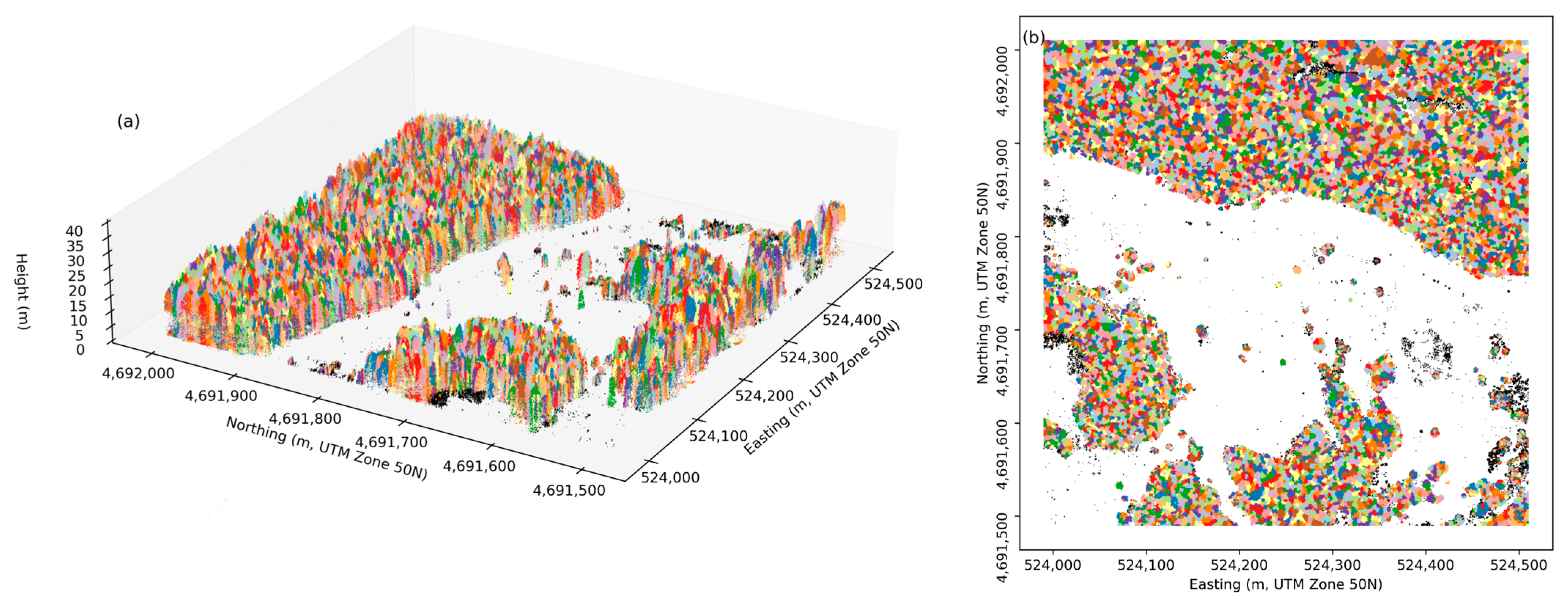
To derive tree density metrics comparable to field inventories, the airborne LiDAR point cloud data were processed to delineate individual trees. The segmentation was performed using an optimized approach that integrates the classical watershed (WS) algorithm with the connection center evolution (CCE) algorithm (Figure 3) [33].
This improved segmentation approach takes full advantage of the high efficiency of WS and the segmentation accuracy of CCE. It is robust in handling complex forest structures and exhibits low sensitivity to parameter settings. Moreover, tree locations and heights can be automatically extracted and output directly, making it a reliable and practical tool for large-scale forest inventory applications. In addition, its application in Saihanba demonstrated higher individual tree segmentation accuracy compared to using either method alone [34].
For quantitative analysis, individual tree point clouds were projected onto a two-dimensional (2D) plane (Figure 4), and the convex hull of each tree was computed to represent its canopy coverage, serving as the basis for density calculations.
In addition, within the airborne LiDAR coverage area, we performed tree species classification for each individual tree (Figure 5) based on 50 indicators describing texture, structural, and spectral characteristics, extracted from CCD imagery and point cloud data [35]. Specifically, the classification utilized 9 structural features derived from LiDAR point clouds, 14 spectral features calculated from hyperspectral imagery, and 27 texture features extracted from orthophotos.
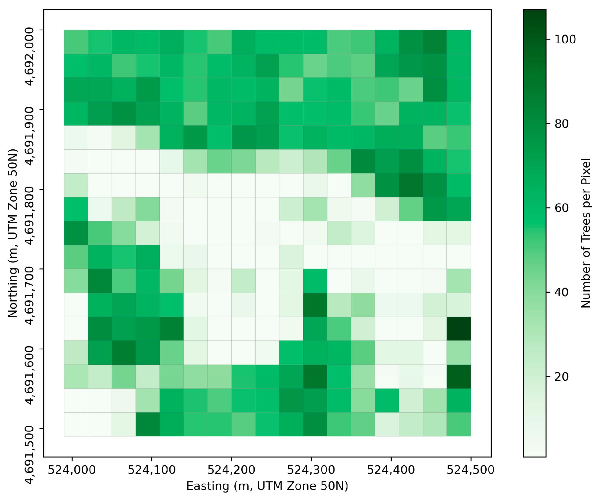
To generate reference data for model training and validation, a 30 m × 30 m vector grid was established over the study area, spatially aligning with the Landsat pixel framework. Within each grid cell, the number of individual tree crowns—extracted from the segmented LiDAR point cloud—was counted (Figure 6). These crown counts served as reference values for model development and validation, enabling a direct comparison between satellite-derived features and ground-based forest structure at the pixel level.

3.3. Random Forest Regression

Random Forest is an ensemble learning algorithm commonly used for both classification and regression tasks [35]. It builds multiple decision trees and averages their predictions to improve accuracy and reduce overfitting. During training, the algorithm creates bootstrap samples from the original dataset and constructs decision trees based on randomly selected features at each node. This randomness increases model diversity and robustness. Additionally, Random Forest provides feature importance rankings, which help identify the most influential variables. In regression tasks, the final output is the average of all decision trees’ predictions. Hyperparameters such as the number and depth of trees can be tuned to optimize model performance.

3.4. Support Vector Regression

SVM is a supervised learning model that constructs an optimal hyperplane to maximize the margin between different classes [36]. Support Vector Regression (SVR) extends this idea to regression problems by introducing an “ε-insensitive” loss function, which allows for small deviations between predicted and actual values. By using kernel functions to map inputs into high-dimensional spaces, SVR can capture nonlinear relationships. During training, only the errors that exceed the ε margin are penalized, enhancing the model’s generalization ability. With proper tuning of ε and other parameters, SVR can perform well on high-dimensional datasets. Specifically, the kernel type defines the transformation applied to input features, affecting the model’s ability to capture nonlinearity; the penalty coefficient C adjusts the trade-off between model complexity and error tolerance; and the kernel width γ , especially for RBF kernels, controls the influence of individual data points on the regression function.

3.5. XGBoost Regression

XGBoost is an ensemble algorithm based on the gradient boosting framework [37]. It iteratively builds weak learners—typically decision trees—by fitting them to the residuals of the previous iteration to improve prediction accuracy. The objective function in XGBoost includes both a loss term (training error) and a regularization term to penalize model complexity and prevent overfitting. Each new tree is trained on the residual errors of the ensemble built so far and is added to the model to incrementally enhance performance. Compared to traditional decision trees, XGBoost includes advanced optimization techniques and is widely used in both regression and classification tasks. With proper parameter tuning, it often yields high-accuracy results.

3.6. Model Evaluation Metrics

3.6.1. Coefficient of Determination (R2)

R2 is a statistical measure used to evaluate how well a regression model explains the variability of the dependent variable. It is defined as follows:
R 2 = 1 S S r e s S S t o t ,
where S S r e s is the residual sum of squares and S S t o t is the total sum of squares. And an R2 value closer to 1 indicates that the model has a better fit, while a value closer to 0 suggests poor explanatory power.

3.6.2. Root Mean Square Error (RMSE)

RMSE measures the average magnitude of the prediction error. It is defined as follows:
R M S E = s q r t 1 n Σ y i ŷ i 2 ,
where y i is the observed value, ŷ i is the predicted value, and n is the number of samples. A smaller RMSE indicates higher prediction accuracy and better model performance. As a direct measure of error magnitude, RMSE is both intuitive and interpretable.
Together, R2 and RMSE provide a comprehensive evaluation of model performance, helping to assess both the goodness of fit and the magnitude of prediction errors, thereby offering reliable support for further analysis and application.

4. Results

4.1. Model Accuracy Evaluation

The three models, Random Forest, SVM, and XGBoost, were trained on 70% of the available reference data. Their predictive performance in forest density inversion was compared on the independent test set using fitting accuracy and error metrics. The test set comprised a total of 54,603 samples.
For the Random Forest model, parameter tuning indicated that the number of decision trees had a significant impact on model accuracy. When the number of trees was set to 300, the model achieved optimal performance, with an R2 of 0.618 and an RMSE of 183 trees ha−1, demonstrating good overall fit. The resulting scatterplot shows most predictions tightly clustered around the 1:1 line, indicating reliable estimates across the full density range.
For the SVM model, a grid search was applied to optimize the kernel type, penalty coefficient C , and kernel width γ . The tuned model achieved an R2 of 0.555 and an RMSE of 197 trees ha−1 on the test set, while the overall error remained acceptable, the algorithm systematically underestimated in high-density areas, limiting its suitability in extreme-value zones.
Because the XGBoost model contains a large hyperparameter space, an exhaustive grid search was also conducted. The final configuration delivered an R2 of 0.653 and an RMSE of 174 trees ha−1, making it the best performer among the three models. Its high accuracy benefited from built-in regularization and dynamic feature weighting mechanisms. The prediction scatterplot confirms consistent accuracy and good generalization across most density levels.
Overall, all three models demonstrated strong predictive capability in this study (Figure 7) and credible regional-scale estimates of forest density. XGBoost achieves the highest accuracy and surpasses the accuracy reported by Chrysafis et al. [11] for single-image or dual-season inputs. Furthermore, its R2 and RMSE values were comparable to those reported by Cheng et al. [38], indicating the model’s potential applicability for density inversion studies in other years.

4.2. Time-Series Results and Analysis

Using the trained XGBoost model, forest density in the Saihanba area was estimated every five years from 1988 to 2023. The resulting density maps are shown in Figure 8.
Overall, the forest density in the Saihanba Forest Farm showed a steadily increasing trend, with the most pronounced gains occurring in the western portion, where large stands of planted forest dominate [27]. This spatial pattern confirms the tangible success of the region’s sustained afforestation programs.
Figure 9 illustrates the temporal evolution of average tree density across the study area. Over the 35-year period, the multi-year trend is characterized by a short-term fluctuation superimposed on a robust long-term increase, reflecting the cumulative impact of Saihanba’s large-scale afforestation initiatives. The average tree density rose from approximately 521 trees ha−1 in 1988 to 628 trees ha−1 in 2023, a net gain of 20.6%. The declines in 1993 and 2013 likely correspond to the park’s establishment and the severe drought in 2012, respectively. Nonetheless, the long-term trend highlights sustained ecological recovery and continuous structural optimization.
In summary, the regional average tree density has steadily increased since the late 20th century, with a particularly accelerated growth in the early 21st century. This change reflects not only the overall success of ecological restoration but also the on-the-ground effectiveness of regional forest management policies and ecological engineering programs.

4.3. Forest Density Changes Across Ecological Function Zones

Saihanba Forest Farm has long implemented afforestation initiatives. Under continued ecological restoration and forestation policies, forest density has gradually increased (Figure 10).
From 1988 to 2023, all three functional zones exhibited dynamic changes in average tree density. The Core Zone consistently had the highest density, increasing from about 470 trees ha−1 in 1988 to 680 trees ha−1 in 2023, a rise of 44.9%. Notably, post-2003, the growth rate accelerated, reflecting the positive impact of strict protection policies. The Buffer Zone also showed steady recovery, increasing from a low point of 443 trees ha−1 in 1993 to 640 trees ha−1 in 2023, marking a 40.4% increase, indicating enhanced ecological buffering capability.
In contrast, the Experimental Zone exhibited more fluctuation. Tree density declined from 1988 to 1998, then rebounded sharply in 2003 to 529 trees ha−1. However, the sharp decline in tree density to 408 trees ha−1 in 2013—the lowest level during the observation period—was likely a consequence of the severe drought in 2012. This interpretation is consistent with the high-intensity disturbance patterns reported by Tao et al. for the same year [27]. By 2023, density had recovered to 545 trees ha−1, suggesting partial restoration of ecological capacity.

4.4. Forest Density Changes Across Slope Gradients

The total tree counts across slope gradients from 1988 to 2023 are shown in Figure 11. All slope zones exhibited varying degrees of increase and fluctuation in total tree numbers, with noticeable differences by slope, indicating the role of terrain in regulating forest succession.
The 0–5° zone saw total tree numbers decrease from approximately 16 million in 1988 to 14 million in 1993, then gradually rise to 18 million by 2023, the highest among all slope classes. The early decline may relate to agricultural land conversion, while later recovery reflects the positive impact of ecological policies and vegetation restoration efforts.
The 5–15° zone began at 17 million in 1988, dropped in 1993, then recovered steadily to 19.6 million by 2023—representing the largest and most stable increase. This slope class appears most favorable for combined natural and artificial vegetation restoration.
The 15–30° zone exhibited more complex patterns. Tree count fell from 13 million in 1988 to 12 million in 1993, recovered to 14 million by 2003, and peaked at 17 million in 2013. However, slight declines followed, reaching 15 million in 2023. The strong coupling of density increases with vegetation restoration suggests vulnerability to natural disturbances like landslides or extreme weather.
The >30° zone showed overall growth, from 2.0 to 2.4 million trees—a rise of 18.9%. Although it has the lowest absolute number, its growth trend is stable, especially between 2003 and 2013, indicating that enclosure and natural succession can be effective even in steep terrains. This area has high conservation potential due to low human disturbance.
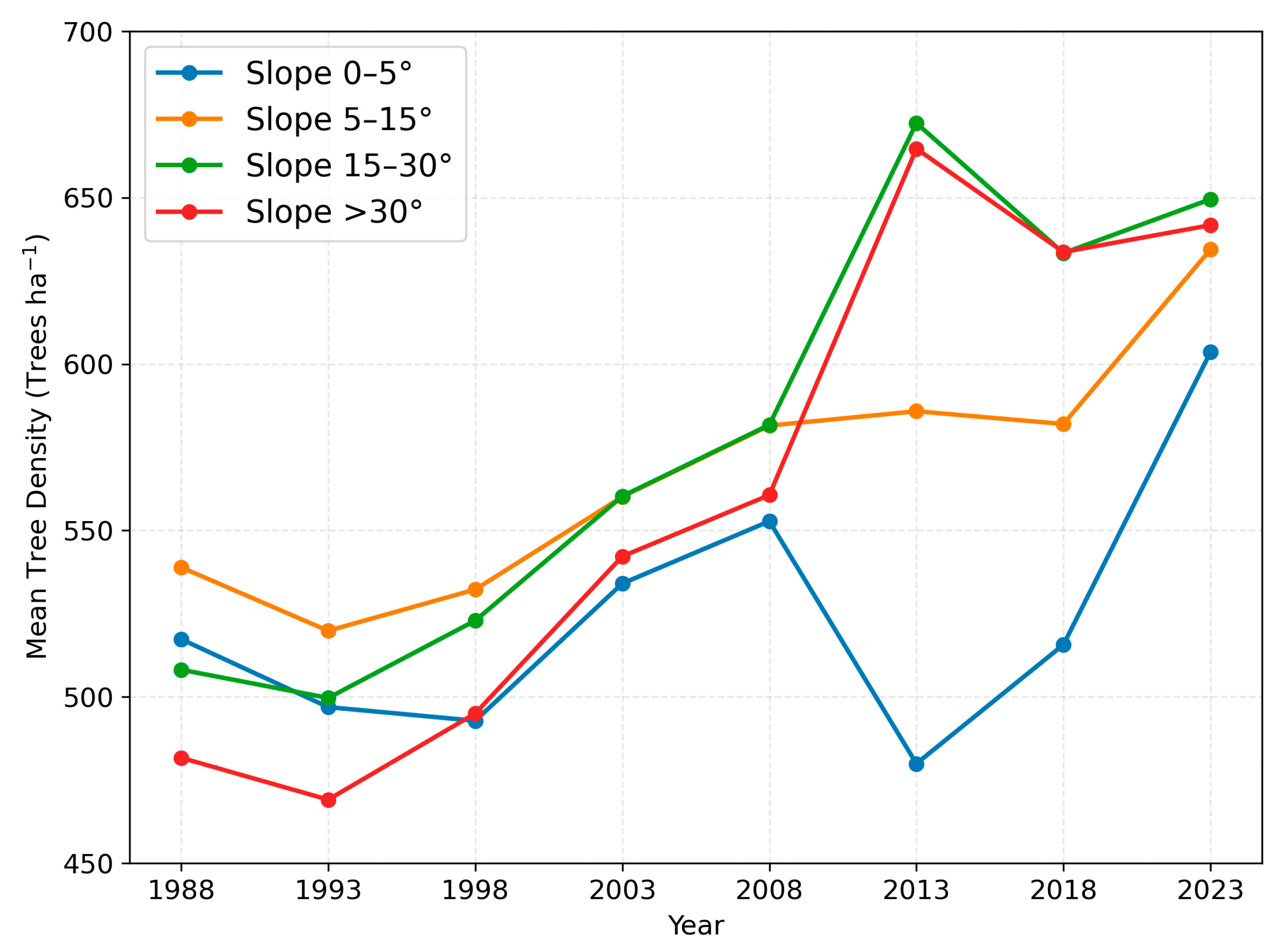
Figure 12 presents the time-series variation of mean forest density across different slope gradients. From 1988 to 2023, average tree density increased in all slope categories, though with varying magnitudes, fluctuations, and inflection points, indicating spatial heterogeneity.
In the 0–5° gentle slope areas, tree density slightly declined from 517 trees ha−1 in 1988 to 493 trees ha−1 in 1998, then gradually increased to 604 trees ha−1 in 2023. Despite the overall upward trend, there was a noticeable drop in 2013 (480 trees ha−1), possibly reflecting frequent land-use activities or higher susceptibility to disturbance. This zone’s gentle terrain typically experiences more human activity, and fluctuations in density may be closely linked to shifts in land management or development pressure.
The 5–15° slope areas showed consistent and steady growth throughout the time series, rising from 539 trees ha−1 in 1988 to 635 trees ha−1 in 2023. Especially after 2003, density increased steadily without major setbacks. This moderate slope zone offers favorable terrain for both mechanical operations and erosion control, likely providing stable conditions for vegetation recovery.
The 15–30° slope zone exhibited the largest increase in density, from 508 trees ha−1 in 1988 to 650 trees ha−1 in 2023, a 27.8% rise. Particularly from 2008 to 2013, density surged from 581.75 to 672.40 trees ha−1, demonstrating strong recovery potential. This middle-mountain zone benefits from relative natural isolation and lower human disturbance, enhancing its capacity for natural regeneration.
In the >30° steep slope zone, tree density increased from 482 to 642 trees ha−1—a 33.2% rise. Growth was relatively stable, with a sharp increase after 2003 and a peak in 2013 (665 trees ha−1). This trend likely reflects the success of enclosure protection and natural succession, while the steep terrain and difficulty of access have limited human impact, making it a vital area for density improvement.
Overall, despite some year-to-year fluctuations, all slope classes experienced long-term increases in tree density, suggesting that forest recovery has been broadly successful under ecological policy and engineering efforts. Initially (in 1988), afforestation primarily occurred on gentle and moderate slopes (0–15°). Over time, activities expanded into steeper areas (15–30° and >30°), where forest density grew rapidly, reflecting the enhanced adaptability of ecological projects in complex terrains.

5. Discussion

5.1. Impact of Tree Species on Training Error

To further analyze potential sources of training error in the XGBoost model, we conducted a species-specific error analysis on the test set using existing tree species classification data over the airborne flight areas [31].
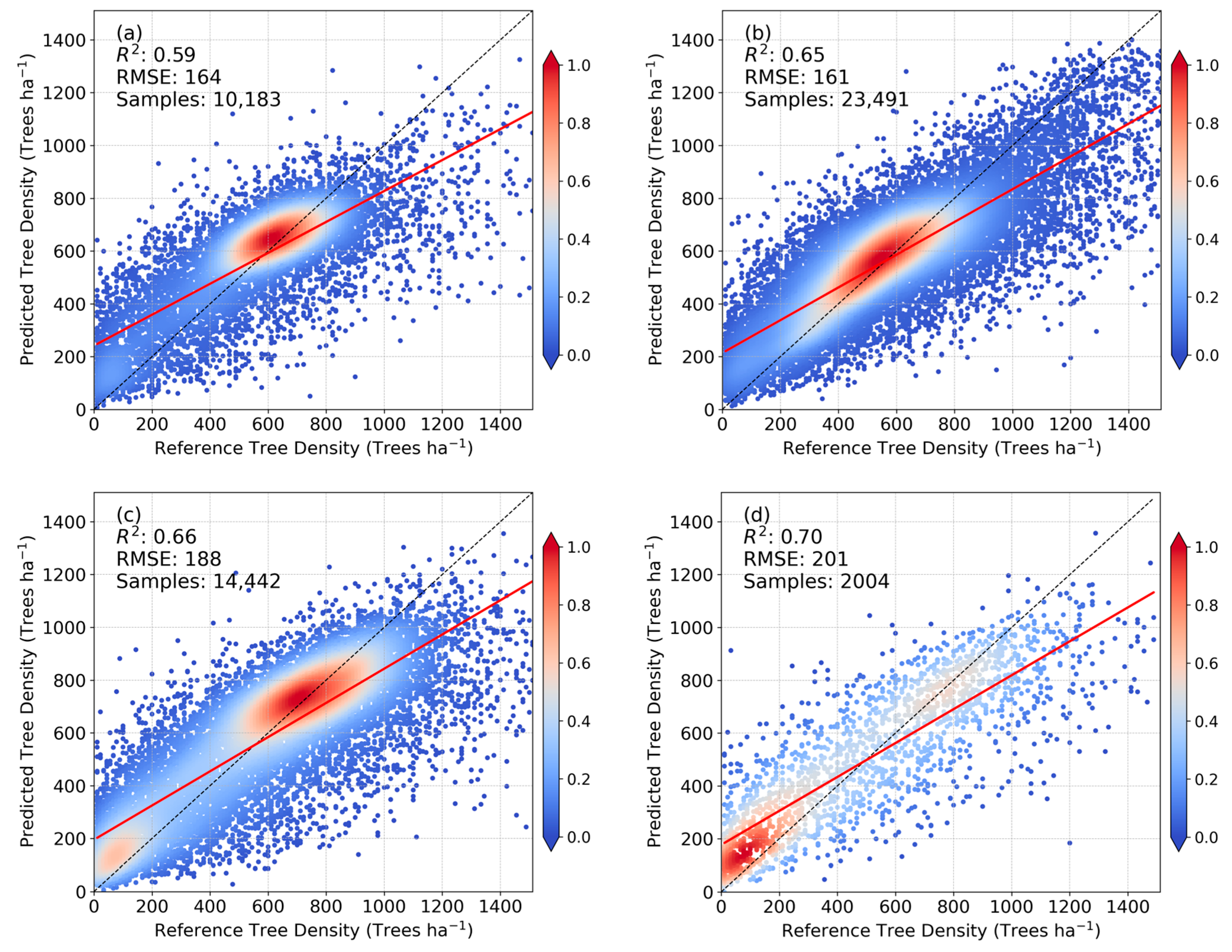
Figure 13 compares the predictive performance for the four tree species. The test set was sampled randomly, with relatively balanced proportions among the four tree species.
It can be seen that spruce, which is sparsely distributed in the study area, produced the highest RMSE (201 trees ha−1), a consequence of its limited representation in both training and test data. Larch, the most widespread species, yielded the lowest error (RMSE = 161 trees ha−1) and hence the highest accuracy. Birch and Mongolian pine occur at comparable frequencies, yet birch’s RMSE (164 trees ha−1) is markedly lower. This discrepancy likely arises because birch dominates the natural forest matrix, whereas Mongolian pine is predominantly planted. Moreover, many Mongolian pine stands consist of seedlings whose small crowns are poorly resolved by the individual tree segmentation algorithm, further elevating prediction error.
Although slight accuracy differences exist among species, their influence on overall density estimates is minor; error magnitude is dictated primarily by training-sample size. Compared with the study by Humagain et al., which employed linear regression, our model achieved higher R2 values for individual species, further demonstrating the superior fitting capacity of the machine learning approach adopted in this study [10]. Provided sufficient species-specific training data in the future, a stratified modeling approach could be adopted to enhance per-species prediction precision.

5.2. Impact of Seasonal Data Configuration on Training Error

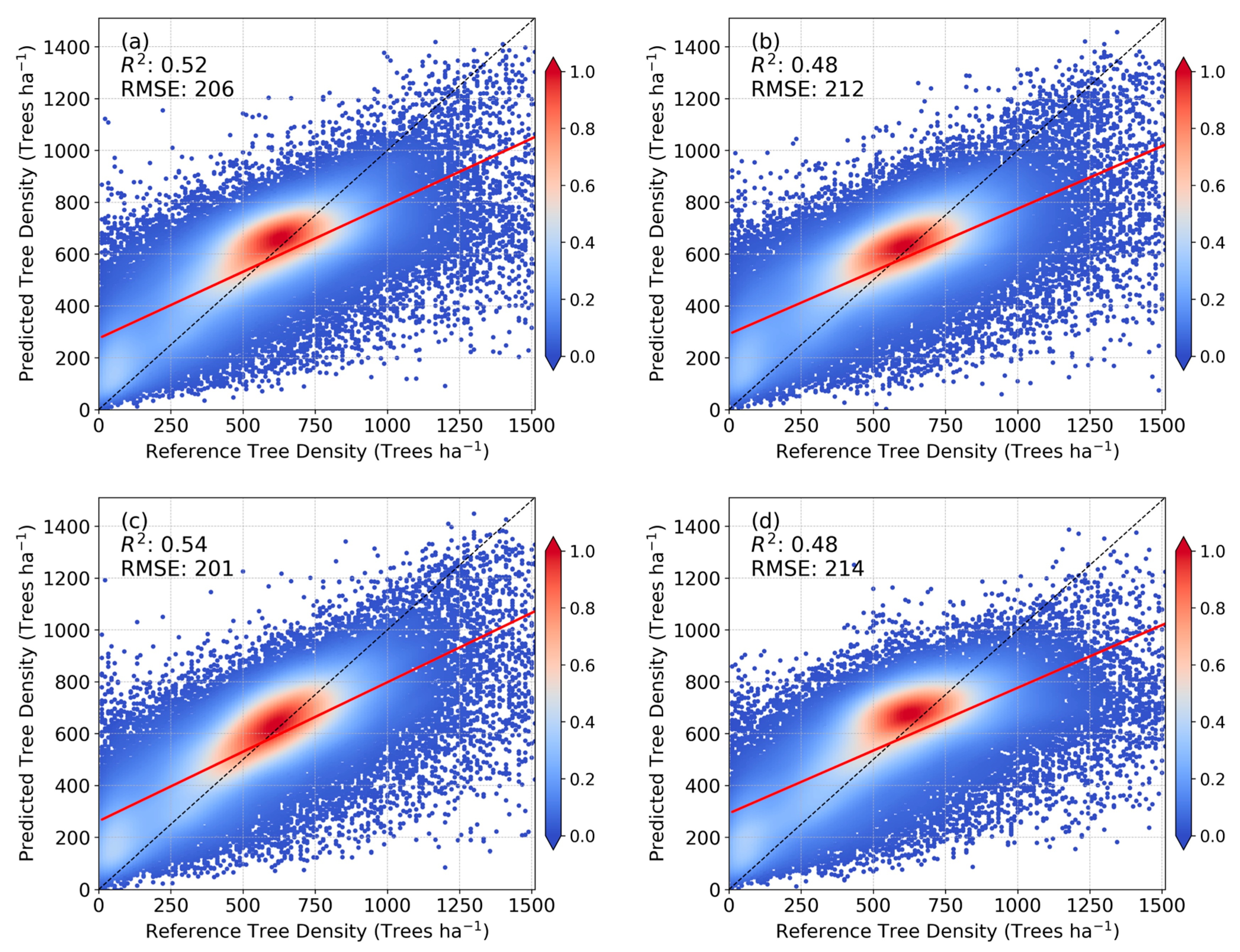
To assess the impact of single-season versus multi-season data on model performance, the XGBoost algorithm was trained independently using datasets from spring, summer, autumn, and winter. The comparative results are presented in Figure 14, with subplots (a) through (d) illustrating scatter plots for each season.
Models trained on single-season data exhibited moderate predictive accuracy, with R2 values ranging from 0.48 to 0.54 and RMSE values between 206 and 214 trees ha−1. The autumn-based model showed slightly better performance; however, overall differences among seasons were limited. These findings suggest that single-season snapshots may be insufficient to capture the temporal variability and ecological complexity influencing tree density. In comparison with the tree density estimation model proposed by Chrysafis et al., which integrated UAV imagery and satellite data, our approach—leveraging airborne LiDAR in combination with satellite imagery—demonstrated superior performance even when constrained to single-season inputs [11]. Specifically, the test set R2 values obtained in our study exceeded those reported for satellite-based predictions in their work, highlighting the enhanced predictive capability afforded by LiDAR integration under limited temporal conditions [11].
By contrast, the model trained with integrated multi-seasonal features achieved a substantially higher R2 of 0.65 and a lower RMSE of 174 trees ha−1, indicating that integrating seasonal features—particularly spectral and vegetation indices—enhances predictive performance. This underscores the value of multi-temporal remote sensing in forest density estimation. For afforestation regions like Saihanba, characterized by distinct seasonal transitions, this approach offers a robust framework for long-term ecological monitoring and restoration assessment.

5.3. Spatial Distribution of Tree Density Change Rates

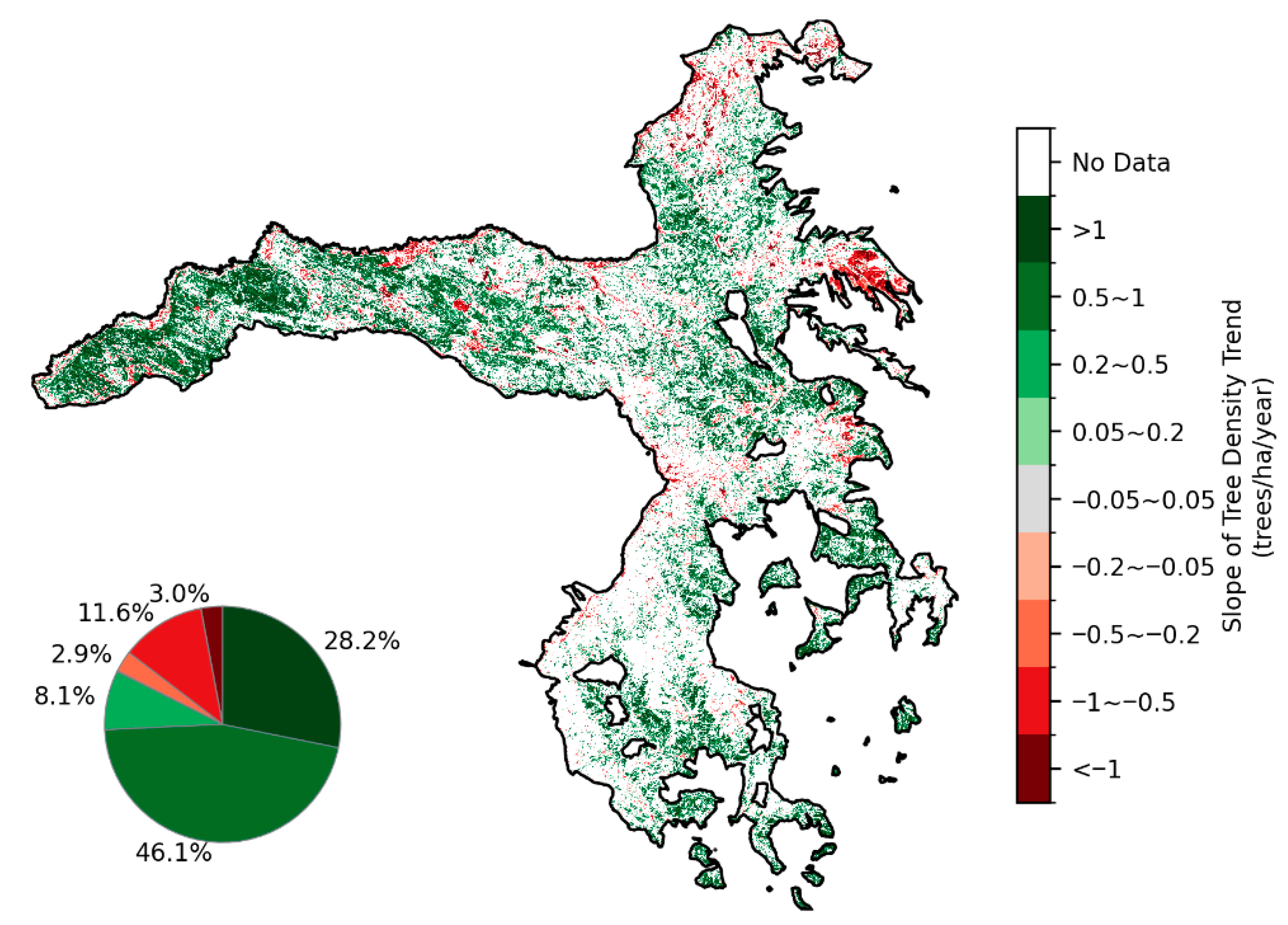
A multi-year linear regression was performed on each pixel to calculate the slope of tree density change, with the spatial distribution shown in Figure 15.
Based on slope calculations for each pixel from 1988 to 2023, most of the study area exhibited positive trends in tree density. Excluding areas with missing data and non-significant trends (p > 0.1), approximately 356,947 valid pixels were included. Of these, 294,291 pixels (82.4%) had positive slopes, with 100,516 pixels (28.2%) showing slopes >1 and 164,614 (46.1%) between 0.5 and 1. This suggests significant density increases across much of the region, indicating the success of long-term ecological restoration and reforestation projects. Compared with the study by Zhang et al., our use of more extensive airborne LiDAR survey data provided a robust foundation for large-scale forest assessment, enabling spatial analysis of tree recovery trends across the Saihanba Forest Farm [9].
Conversely, 62,656 pixels (17.5%) had negative slopes. Of these, 10,569 pixels showed steep declines (slope < −1), likely due to natural disturbances, pests, or human activities like logging. Most negative-change pixels (41,559) fell within the −1 to −0.5 range. Spatially, negative trends were mainly concentrated in the northern artificial forest areas, consistent with findings by Tao et al. [27].
Notably, no pixels exhibited near-zero trends (slope between −0.05 and 0.05), indicating almost no areas with stable long-term density across four decades—most areas underwent significant dynamic changes.
In conclusion, the regional forest structure has undergone notable temporal evolution over the past 40 years, dominated by positive growth. This reflects the effective role of ecological policies in forest recovery. However, localized declines highlight the need for continued monitoring and targeted management to ensure the long-term stability and sustainability of the ecosystem.

6. Conclusions

This study employed airborne LiDAR-derived tree density as a reference and extracted 96 seasonal features from Landsat SR products, including commonly used vegetation indices NDVI and EVI, to train a regression model for estimating tree density. Among several tested machine learning algorithms, the XGBoost model demonstrated the best performance, with an R2 of 0.65 and an RMSE of 174 trees ha−1 on the test set, outperforming both SVR and Random Forest models. The overall prediction accuracy was satisfactory, with relatively low error and strong model generalization.
However, the scatter plot revealed a tendency to underestimate higher values, suggesting that further analysis and model optimization are needed for areas with high tree density. This underestimation may be attributed to the saturation of reflectance in optical bands. Future work could consider incorporating microwave data, such as Sentinel-1, to improve estimation accuracy in densely forested regions. Furthermore, future research may further explore the spatial heterogeneity of density changes and their interactions with topography, land-use history, and human disturbance intensity to construct a more comprehensive framework for evaluating forest restoration dynamics.
Using the trained model, forest density was estimated at five-year intervals from 1988 to 2023. The results indicate a general increasing trend with fluctuations, which is closely related to long-term afforestation policies and ecological restoration efforts in the Saihanba region. These findings highlight the effectiveness of artificial forest management in promoting forest ecosystem recovery.
Overall, this study demonstrates that integrating multiple vegetation indices with an XGBoost model can effectively estimate and monitor changes in tree density over large areas. Although there is still room for improvement in high-value predictions, the model shows solid performance. Future work can further enhance prediction accuracy and generalization by incorporating additional features such as topography, climate, and historical disturbances, and by applying more advanced machine learning architectures. As richer and more diverse datasets become available, we plan to apply deep learning methods such as convolutional neural networks (CNNs) to better capture spatial complexity and ecological patterns. Given that the current airborne LiDAR coverage is concentrated in relatively flat terrain, future studies should consider integrating more comprehensive measurement data to enable more detailed topographic analysis. These results provide valuable scientific support for ecological conservation and forest resource management.

Author Contributions

Funding acquisition, D.X.; software, N.W.; writing—original draft, N.W.; writing—review and editing, D.X.; investigation, L.J. and Y.L.; supervision, G.Y. and X.M. All authors have read and agreed to the published version of the manuscript.

Funding

The work is funded by the National Key Research and Development Program of China (Grant No. 2022YFB3903304) and the National Natural Science Foundation of China (Grant No. 42471376).

Data Availability Statement

Not applicable.

Acknowledgments

The authors thank Si Gao, Bang Sun, and Qian Wang for giving nice suggestions and help.

Conflicts of Interest

The authors declare no conflicts of interest.

References

  1. Xu, X.L.; Cao, M.K.; Li, K.R. Temporal-Spatial Dynamics of Carbon Storage of Forest Vegetation in China. Prog. Geogr. 2007, 26, 1–10. [Google Scholar]
  2. Dubrovin, I.; Fortin, C.; Kedrov, A. An open dataset for individual tree detection in UAV LiDAR point clouds and RGB orthophotos in dense mixed forests. Sci. Rep. 2024, 14, 21938. [Google Scholar] [CrossRef]
  3. Zeide, B. How to Measure Stand Density. Trees 2005, 19, 1–14. [Google Scholar] [CrossRef]
  4. Hansen, M.C.; Potapov, P.V.; Moore, R.; Hancher, M.; Turubanova, S.A.; Tyukavina, A.; Thau, D.; Stehman, S.V.; Goetz, S.J.; Loveland, T.R.; et al. High-Resolution Global Maps of 21st-Century Forest Cover Change. Science 2013, 342, 850–853. [Google Scholar] [CrossRef] [PubMed]
  5. Fassnacht, F.E.; Mangold, D.; Schäfer, J.; Immitzer, M.; Kattenborn, T.; Koch, B.; Latifi, H. Estimating Stand Density, Biomass and Tree Species from Very High Resolution Stereo-Imagery–Towards an All-in-One Sensor for Forestry Applications? Forestry 2017, 90, 613–631. [Google Scholar] [CrossRef]
  6. Guo, W.; Yang, C.Y.; Wu, Z.R.; Ji, X.L.; Yang, C.J.; Zhao, C.W.; Zhang, Y.H. Forest Density Mapping Based on UAV High-Resolution Image. Bull. Surv. Map. 2021, 07, 29–33. [Google Scholar] [CrossRef]
  7. Sun, H.; Guo, X.Y.; Zhang, H.Y.; Zhao, J.J. Estimating Canopy Bulk Density and Canopy Base Height Using UAV LiDAR and Multispectral Images. Natl. Remote Sens. Bull. 2024, 28, 3107–3122. [Google Scholar] [CrossRef]
  8. Crowther, T.W.; Glick, H.B.; Covey, K.R.; Bettigole, C.; Maynard, D.S.; Thomas, S.M.; Smith, J.R.; Hintler, G.; Duguid, M.C.; Amatulli, G.; et al. Mapping Tree Density at a Global Scale. Nature 2015, 525, 201–205. [Google Scholar] [CrossRef] [PubMed]
  9. Zhang, Z.; Dong, X.; Tian, J.; Tian, Q.; Xi, Y.; He, D. Stand Density Estimation Based on Fractional Vegetation Coverage from Sentinel-2 Satellite Imagery. Int. J. Appl. Earth Obs. Geoinf. 2022, 108, 102760. [Google Scholar] [CrossRef]
  10. Humagain, K.; Portillo-Quintero, C.; Cox, R.; Cain, J. Mapping Tree Density in Forests of the Southwestern USA Using Landsat 8 Data. Forests 2017, 8, 287. [Google Scholar] [CrossRef]
  11. Chrysafis, I.; Mallinis, G.; Gitas, I.; Tsakiri-Strati, M. Estimating Mediterranean Forest Parameters Using Multi Seasonal Landsat 8 OLI Imagery and an Ensemble Learning Method. Remote Sens. Environ. 2017, 199, 154–166. [Google Scholar] [CrossRef]
  12. Sivanpillai, R.; Smith, C.T.; Srinivasan, R.; Messina, M.G.; Wu, X.B. Estimation of Managed Loblolly Pine Stand Age and Density with Landsat ETM+ Data. For. Ecol. Manag. 2006, 223, 247–254. [Google Scholar] [CrossRef]
  13. LaRue, E.; Wagner, F.; Fei, S.; Atkins, J.; Fahey, R.; Gough, C.; Hardiman, B. Compatibility of Aerial and Terrestrial LiDAR for Quantifying Forest Structural Diversity. Remote Sens. 2020, 12, 1407. [Google Scholar] [CrossRef]
  14. White, J.C.; Coops, N.C.; Wulder, M.A.; Vastaranta, M.; Hilker, T.; Tompalski, P. Remote Sensing Technologies for Enhancing Forest Inventories: A Review. Can. J. Remote Sens. 2016, 42, 619–641. [Google Scholar] [CrossRef]
  15. Packalen, P.; Vauhkonen, J.; Kallio, E.; Peuhkurinen, J.; Pitkänen, J.; Pippuri, I.; Strunk, J.; Maltamo, M. Predicting the Spatial Pattern of Trees by Airborne Laser Scanning. Int. J. Remote Sens. 2013, 34, 5154–5165. [Google Scholar] [CrossRef]
  16. Pang, Y.; Li, Z.; Ju, H.; Lu, H.; Jia, W.; Si, L.; Guo, Y.; Liu, Q.; Li, S.; Liu, L.; et al. LiCHy: The CAF’s LiDAR, CCD and Hyperspectral Integrated Airborne Observation System. Remote Sens. 2016, 8, 398. [Google Scholar] [CrossRef]
  17. Mohammadi, J.; Shataee Joibary, S.; Yaghmaee, F.; Mahiny, A.S. Modelling Forest Stand Volume and Tree Density Using Landsat ETM+ Data. Int. J. Remote Sens. 2010, 31, 2959–2975. [Google Scholar] [CrossRef]
  18. Bulut, S.; Günlü, A.; Çakır, G. Modelling Some Stand Parameters Using Landsat 8 OLI and Sentinel-2 Satellite Images by Machine Learning Techniques: A Case Study in Türkiye. Geocarto Int. 2023, 38, 2158238. [Google Scholar] [CrossRef]
  19. Joshi, C.; Leeuw, J.D.; Skidmore, A.K.; Duren, I.C.V.; van Oosten, H. Remotely Sensed Estimation of Forest Canopy Density: A Comparison of the Performance of Four Methods. Int. J. Appl. Earth Obs. Geoinf. 2006, 8, 84–95. [Google Scholar] [CrossRef]
  20. Kahriman, A.; Günlü, A.; Karahalil, U. Estimation of Crown Closure and Tree Density Using Landsat TM Satellite Images in Mixed Forest Stands. J. Indian Soc. Remote Sens. 2014, 42, 559–567. [Google Scholar] [CrossRef]
  21. Sismanis, M.; Gitas, I.Z.; Georgopoulos, N.; Stavrakoudis, D.; Gkounti, E.; Antoniadis, K. A Spectral–Spatial Approach for the Classification of Tree Cover Density in Mediterranean Biomes Using Sentinel-2 Imagery. Forests 2024, 15, 2025. [Google Scholar] [CrossRef]
  22. Su Mon, M.; Mizoue, N.; Htun, N.Z.; Kajisa, T.; Yoshida, S. Estimating Forest Canopy Density of Tropical Mixed Deciduous Vegetation Using Landsat Data: A Comparison of Three Classification Approaches. Int. J. Remote Sens. 2012, 33, 1042–1057. [Google Scholar] [CrossRef]
  23. Yang, H.; Wang, S.; Son, R.; Lee, H.; Benson, V.; Zhang, W.; Zhang, Y.; Zhang, Y.; Kattge, J.; Boenisch, G.; et al. Global Patterns of Tree Wood Density. Glob. Change Biol. 2024, 30, e17224. [Google Scholar] [CrossRef]
  24. Lozano-Tello, A.; Luceño, J.; Caballero-Mancera, A.; Clemente, P.J. Estimating Olive Tree Density in Delimited Areas Using Sentinel-2 Images. Remote Sens. 2025, 17, 508. [Google Scholar] [CrossRef]
  25. Mouafik, M.; Mounir, F.; Aboudi, A.E. Integrating Multi-Source Remote Sensing Data and Machine Learning for Predicting Tree Density and Cover in Argania spinosa. Smart Agric. Technol. 2025, 11, 100911. [Google Scholar] [CrossRef]
  26. Kang, J.; Qing, Y.; Lu, W. Construction and Optimization of the Saihanba Ecological Network. Ecol. Indic. 2023, 153, 110401. [Google Scholar] [CrossRef]
  27. Tao, C.; Guo, T.; Shen, M.; Tang, Y. Spatio-Temporal Dynamic of Disturbances in Planted and Natural Forests for the Saihanba Region of China. Remote Sens. 2023, 15, 4776. [Google Scholar] [CrossRef]
  28. Hu, Y.J.Q.; Xiao, J.; Yu, B.W.; Xu, W.H. Research Progress in Function Zoning of Nature Reserves in China. Acta Ecol. Sin. 2014, 34, 6391–6396. [Google Scholar] [CrossRef]
  29. Zhang, W.; Qi, J.; Wan, P.; Wang, H.; Xie, D.; Wang, X.; Yan, G. An Easy-to-Use Airborne LiDAR Data Filtering Method Based on Cloth Simulation. Remote Sens. 2016, 8, 501. [Google Scholar] [CrossRef]
  30. Wulder, M.A.; White, J.C.; Goward, S.N.; Masek, J.G.; Irons, J.R.; Herold, M.; Cohen, W.B.; Loveland, T.R.; Woodcock, C.E. Landsat Continuity: Issues and Opportunities for Land Cover Monitoring. Remote Sens. Environ. 2008, 112, 955–969. [Google Scholar] [CrossRef]
  31. Wulder, M.A.; White, J.C.; Loveland, T.R.; Woodcock, C.E.; Belward, A.S.; Cohen, W.B.; Fosnight, E.A.; Shaw, J.; Masek, J.G.; Roy, D.P. The Global Landsat Archive: Status, Consolidation, and Direction. Remote Sens. Environ. 2016, 185, 271–283. [Google Scholar] [CrossRef]
  32. Zhu, Z.; Woodcock, C.E. Object-Based Cloud and Cloud Shadow Detection in Landsat Imagery. Remote Sens. Environ. 2012, 118, 83–94. [Google Scholar] [CrossRef]
  33. Li, Y.; Xie, D.; Wang, Y.; Jin, S.; Zhou, K.; Zhang, Z.; Li, W.; Zhang, W.; Mu, X.; Yan, G. Individual Tree Segmentation of Airborne and UAV LiDAR Point Clouds Based on the Watershed and Optimized Connection Center Evolution Clustering. Ecol. Evol. 2023, 13, e10297. [Google Scholar] [CrossRef] [PubMed]
  34. Xie, D.H.; Li, Y.; Zhou, K.; Zhang, Z.X.; Jin, L.; Yan, G.J.; Mu, X.H.; Li, W.H.; Feng, G.Y. Information Extraction and System Construction of Digital Forest System Based on Multisource Remote Sensing Data. Natl. Remote Sens. Bull. 2024, 28, 1281–1294. [Google Scholar] [CrossRef]
  35. Breiman, L. Random Forests. Mach. Learn. 2001, 45, 5–32. [Google Scholar] [CrossRef]
  36. Tian, Y. Support Vector Regression and Its Application. Ph.D. Thesis, China Agricultural University, Beijing, China, 2005. [Google Scholar]
  37. Chen, T.; Guestrin, C. XGBoost: A Scalable Tree Boosting System. In Proceedings of the 22nd ACM SIGKDD International Conference on Knowledge Discovery and Data Mining, San Francisco, CA, USA, 13–17 August 2016; pp. 785–794. [Google Scholar] [CrossRef]
  38. Cheng, K.; Yang, H.; Chen, Y.; Yang, Z.; Ren, Y.; Zhang, Y.; Lin, D.; Liu, W.; Huang, G.; Xu, J.; et al. How Many Trees Are There in China? Sci. Bull. 2025, 70, 1076–1079. [Google Scholar] [CrossRef]
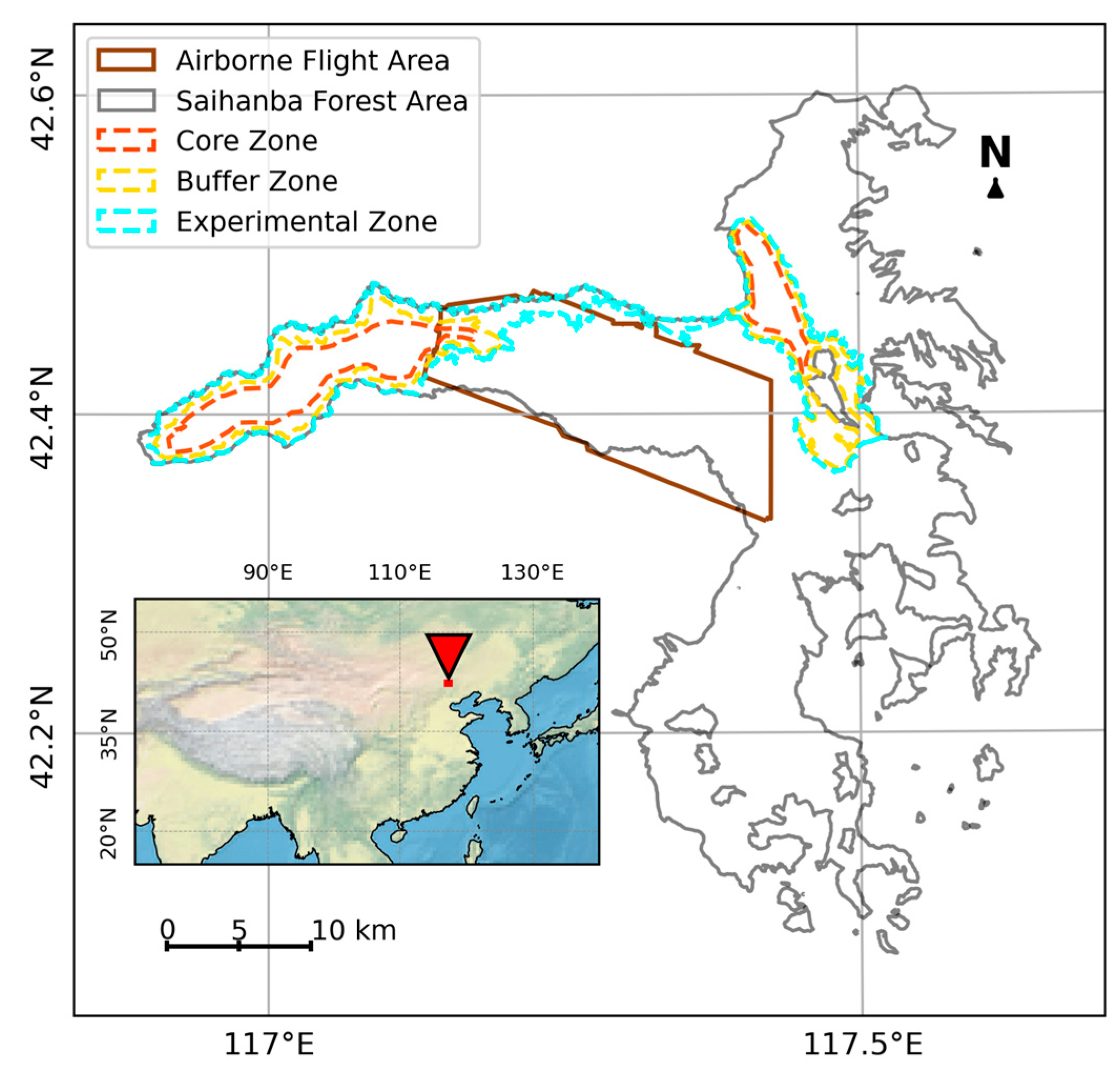
Figure 1. Map of the study area.
Remotesensing 17 03338 g001
Figure 2. Technical Workflow.
Remotesensing 17 03338 g002
Figure 3. Example of individual tree segmentation in a local airborne LiDAR point cloud using the proposed individual tree segmentation method. Different colors represent segmented tree crowns. (a) shows the side view, while (b) shows the top view.
Remotesensing 17 03338 g003
Figure 4. Example of 2D projection of individual tree crown segmentation results from airborne LiDAR data.
Remotesensing 17 03338 g004
Figure 5. Example of individual tree classification results.
Remotesensing 17 03338 g005
Figure 6. Example of spatial tree crown density distribution within the airborne LiDAR-covered area. Vector grid of 30 m resolution cells, each spatially corresponding to a Landsat pixel, overlaid on the airborne flight area. High-density areas are shown in dark green, and low-density areas in light green.
Remotesensing 17 03338 g006
Figure 7. Validation of model prediction accuracy for (a) Random Forest, (b) SVM, and (c) XGBoost based on the test set.
Remotesensing 17 03338 g007
Figure 8. Forest density maps of Saihanba from 1988 to 2023.
Remotesensing 17 03338 g008
Figure 9. Temporal variation in average forest density in Saihanba.
Remotesensing 17 03338 g009
Figure 10. Average tree density variation across different functional zones.
Remotesensing 17 03338 g010
Figure 11. Total number of trees across slope classes.
Remotesensing 17 03338 g011
Figure 12. Average tree density variation across different slope classes.
Remotesensing 17 03338 g012
Figure 13. Accuracy performance for (a) birch (Betula), (b) larch (Larix), (c) Mongolian pine (Pinus sylvestris var. mongolica), and (d) spruce (Picea) based on the test set.
Remotesensing 17 03338 g013
Figure 14. Accuracy performance across seasons for (a) spring, (b) summer, (c) autumn, and (d) winter based on the test set.
Remotesensing 17 03338 g014
Figure 15. Spatial distribution of tree density change trends (p < 0.1).
Remotesensing 17 03338 g015
Table 1. Selected spectral bands.
BandLandsat 5 TM (μm)Landsat 8 OLI (μm)
BlueBand 1 (0.45–0.52)Band 2 (0.45–0.51)
GreenBand 2 (0.52–0.60)Band 3 (0.53–0.59)
RedBand 3 (0.63–0.69)Band 4 (0.64–0.67)
Near-Infrared (NIR)Band 4 (0.76–0.90)Band 5 (0.85–0.88)
Short-Wave Infrared IBand 5 (1.55–1.75)Band 6 (1.57–1.65)
Short-Wave Infrared IIBand 7 (2.08–2.35)Band 7 (2.11–2.29)
Disclaimer/Publisher’s Note: The statements, opinions and data contained in all publications are solely those of the individual author(s) and contributor(s) and not of MDPI and/or the editor(s). MDPI and/or the editor(s) disclaim responsibility for any injury to people or property resulting from any ideas, methods, instructions or products referred to in the content.