Article

Deep-Learning-Based Probabilistic Forecasting of Groundwater Storage Dynamics in Sudan Using Multisource Remote Sensing and Geophysical Data

by
Musaab A. A. Mohammed
1,2,*,
Norbert P. Szabó
1,
Joseph O. Alao
3 and
Péter Szűcs
1
1
Faculty of Earth and Environmental Sciences and Engineering, University of Miskolc, 3515 Miskolc, Hungary
2
Department of Hydrogeology, College of Petroleum Geology and Minerals, University of Bahri, Khartoum 1660, Sudan
3
Department of Physics, Air Force Institute of Technology, Kaduna 2104, Nigeria
*
Author to whom correspondence should be addressed.
Remote Sens. 2025, 17(18), 3172; https://doi.org/10.3390/rs17183172
Submission received: 12 August 2025 / Revised: 9 September 2025 / Accepted: 11 September 2025 / Published: 12 September 2025

Abstract

Highlights

What are the main findings?
  • The integrated machine learning approach successfully reconstructed gaps in GRACE/GRACE-FO data and produced reliable forecasts of groundwater storage dynamics with quantified uncertainty.
  • Groundwater storage anomalies in Sudan shows a consistent long-term recovery trend, with the strongest increases observed in semi-tropical regions.
What are the implications of the main findings?
  • The developed framework demonstrates how combining satellite observations with machine learning can guide sustainable groundwater monitoring and management in data-scarce and climate-stressed regions.
  • The findings provide new evidence that groundwater is the dominant driver of water storage variability in Sudan, underscoring its critical role in sustaining water supply for domestic and agricultural purposes.

Abstract

Geophysical and remote sensing observations offer powerful means to monitor large-scale hydrological changes, particularly in regions where in situ data are scarce. In this study, we integrate satellite-derived water storage from the Gravity Recovery and Climate Experiment (GRACE) with land surface variables from the Global Land Data Assimilation System (GLDAS) to assess and forecast groundwater storage (GWS) dynamics across eight major regions in Sudan. Missing GRACE observations of terrestrial water storage (TWS) were first reconstructed using a Random Forest machine learning model, after which GWS anomalies were estimated by subtracting GLDAS-based surface and root-zone components from TWS. The resulting GWS time series was decomposed into trend, seasonal, and residual components, and the trend signals were used to train a bootstrapped Bidirectional Long Short-Term Memory (BiLSTM) model. This framework generated probabilistic forecasts accompanied by confidence intervals, which were generally narrow and consistent with the historical range. The forecasted GWS anomalies indicate positive recovery across all regions, with Sen’s slope values ranging from 0.014 to 0.051 per month. The strongest recoveries are evident in the southern and southwestern regions, while northern and eastern areas display more modest gains. This work represents one of the first applications of deep learning with uncertainty quantification for GRACE-based groundwater analysis in Sudan, demonstrating the potential of such an integrated approach to support informed and sustainable groundwater management in data-limited environments.

1. Introduction

Groundwater storage is a fundamental component of the global water cycle that supports a wide range of human and ecological needs, from drinking water and agriculture to river and wetland ecosystems. The significance of groundwater has grown in recent decades due to increasing pressure on surface water from population growth and climate variability [1]. Monitoring changes in groundwater storage is essential, especially in arid and semi-arid regions where groundwater is often the only dependable water source. Traditionally, such monitoring has relied on in situ measurements from well networks. While these provide valuable point-based data, they often suffer from limited spatial coverage, high maintenance costs, and accessibility issues, particularly in remote areas [2]. As a result, there has been growing interest in alternatives such as geophysical and remote sensing techniques for their broader spatial coverage and cost-effective solutions for large-scale groundwater monitoring [3].
In recent years, satellite-based remote sensing has become a transformative approach for monitoring large-scale terrestrial water storage. Notably, the Gravity Recovery and Climate Experiment (GRACE) mission has provided over two decades of continuous observations, offering a temporal record for analyzing long-term trends in groundwater dynamics. GRACE’s capabilities have been validated by the scientific community through comparative studies conducted across diverse hydrogeological settings and climatic conditions worldwide. Extensive validation studies have shown that incorporating GRACE data into groundwater models greatly improves simulation accuracy, when compared with in situ observations [4,5]. GRACE’s reliability for detecting groundwater storage changes at scales ranging from large river basins to continental aquifer systems has been consistently demonstrated through multi-regional validation studies. In Africa, GRACE-based studies have provided critical insights into groundwater storage variability under conditions of high climate stress and limited monitoring infrastructure. For example, Ding et al. [6] applied GRACE and machine learning to assess spatiotemporal variations in groundwater across Africa, while Mohasseb et al. [7] investigated groundwater storage responses to climate change in African river basins. Similar efforts have been made to evaluate transboundary aquifer systems in North Africa and the Sahel, highlighting both depletion risks and the importance of satellite observations in regions with sparse in situ data. Comparable applications in the Middle East [8,9,10] and South Asia [11,12,13] have further confirmed the value of GRACE. Through these comprehensive validation efforts, GRACE has been established as an indispensable tool through which water storage dynamics can be understood.
Recent technological advances have further expanded GRACE’s applications through improved data processing techniques and analytical capabilities. Machine learning (ML) and deep learning (DL) approaches have been successfully integrated with GRACE data across diverse hydroclimatic regions [14]. Most of these studies have primarily focused on addressing data limitations through gap-filling [15,16], enhancing spatial resolution via downscaling methods [17,18,19], and improving groundwater analysis and forecasting [12,20,21]. However, deep learning (DL) models have demonstrated superior performance compared to traditional machine learning approaches, particularly in capturing complex, nonlinear spatiotemporal patterns [22]. Deep learning (DL) refers to a family of neural network models capable of automatically extracting hierarchical feature representations from data [23]. These models are composed of multiple layers of interconnected artificial neurons, where each neuron applies a weighted transformation followed by a nonlinear activation function. This layered structure allows DL to model complex, nonlinear, and high-dimensional relationships more effectively than traditional ML approaches [24]. For hydrological applications, recurrent neural networks (RNNs) and their advanced variants, such as Long Short-Term Memory (LSTM) and Bidirectional LSTM (BiLSTM), are particularly well-suited as they incorporate memory units and gating mechanisms that capture both short- and long-term temporal dependencies [25]. For instance, Yin et al. [26] demonstrated that LSTM model, significantly outperforms traditional machine learning models like Random Forest (RF) and Artificial Neural Networks (ANN) in predicting groundwater levels. Simlariy, Gaffoor et al. [27] demonstrated that LSTM outperformed gradient-boosted decision tree (GBDT) in modeling groundwater level changes, particularly under slightly larger datasets. All these studies have successfully utilized GRACE data for groundwater analysis and forecasting, demonstrating the potential of deep learning models even in data-scarce regions. However, most GRACE-based groundwater studies lack explicit uncertainty quantification, which is a critical omission given the coarse spatial resolution of GRACE, the variability in hydrological conditions, and the limited availability of ground-based validation data. Incorporating uncertainty estimates is essential for ensuring the reliability of predictions and supporting risk-informed groundwater management decisions [28].
Sudan has diverse hydrogeological framework ranging from extensive unconsolidated alluvial deposits to sedimentary aquifers, and crystalline basement formations that exhibits a variety of groundwater storage capacities [29]. These differences highlight the importance of regional-scale assessments that account for hydrogeological and climatic variability. Despite the critical importance of understanding groundwater dynamics in Sudan, few studies have comprehensively assessed the spatiotemporal variations in groundwater storage. Most existing research has been limited to isolated or localized systems, lacking a regional perspective necessary for effective water resource planning and management [30,31,32]. This gap is largely due to the challenges in collecting hydrological data due to sparse monitoring networks and limited access to well-based observations. This study aims to bridge these gaps by analyzing satellite-derived total water storage (TWS) and groundwater storage (GWS) anomalies, together with land surface variables, under diverse hydroclimatic and hydrogeological conditions. The specific objectives are to achieve the following:
  • Fill gaps in the GRACE/GRACE-FO record using land surface variables from, ensuring a continuous time series of TWS and GWS.
  • Analyze long-term trends and variability in GWS anomalies from the completed time series, highlighting regional patterns across different hydroclimatic and hydrogeological settings.
  • Forecast GWS anomalies up to three years beyond the observational record using a Bi-LSTM model and quantify uncertainty through ensemble modeling, providing probabilistic insights into the reliability of the forecasted GWS anomalies.
This integrated framework improves the reliability of groundwater assessments and supports informed water resource management in data-scarce environments.

2. Description of the Study Area

Sudan lies in northeastern Africa, spanning latitudes 4°50′N to 22°30′N and longitudes 21°50′E to 38°45′E, covering an area of about 1.86 million km2 with an average elevation of 600 m above sea level (Figure 1). As the third-largest country in Africa, Sudan exhibits a wide range of geographical features, from dry deserts in the north to greener, more fertile zones in the south. It is bordered by Egypt, Libya, Chad, the Central African Republic, South Sudan, Ethiopia, and Eritrea. Much of the country consists of flat plains, with occasional low hills rising from the Saharan Plateau. Hydrologically, Sudan is defined by the meeting of the White and Blue Nile Rivers in Khartoum, forming the main Nile River that flows north through Egypt into the Mediterranean Sea.
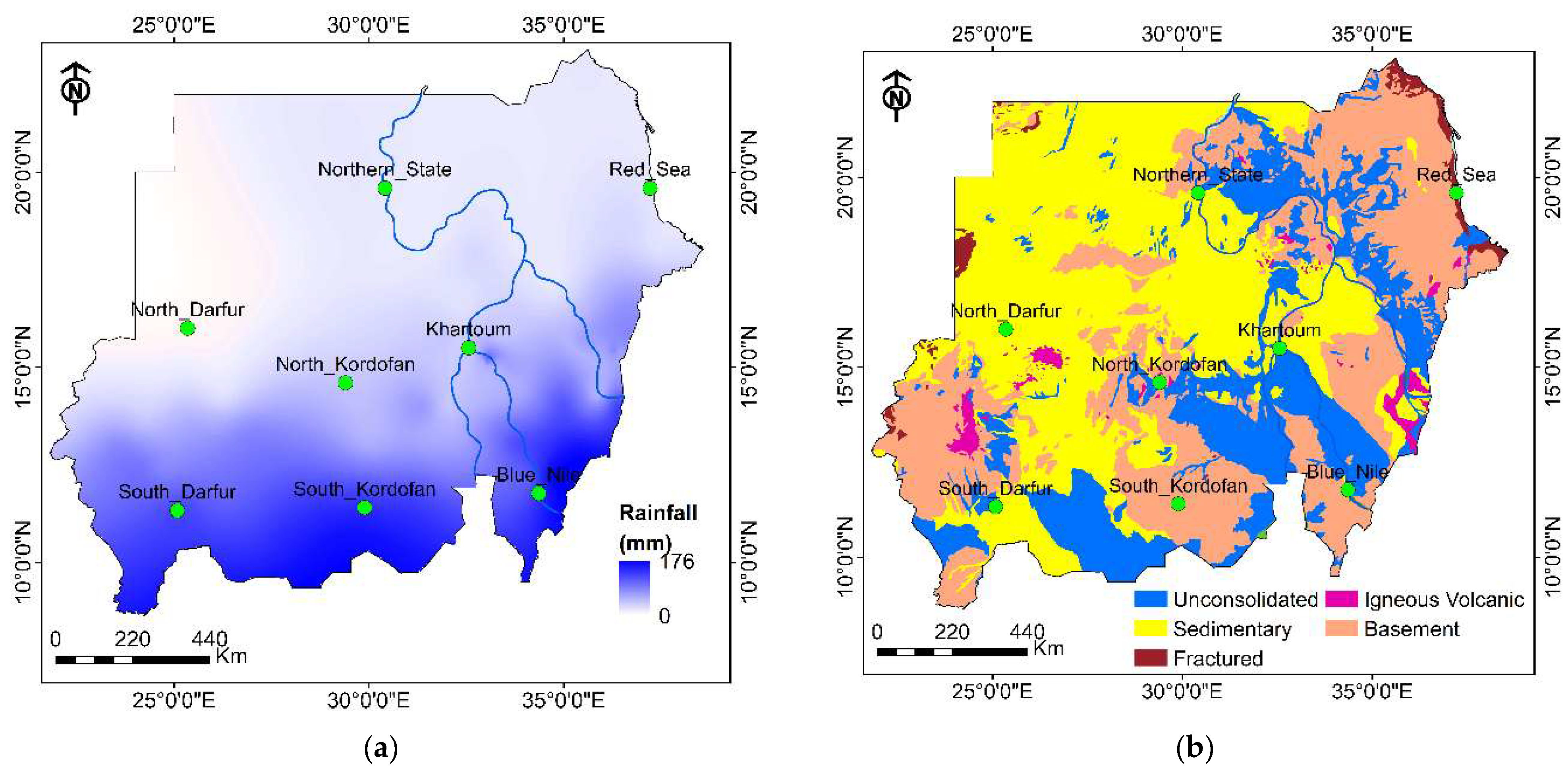
Rainfall in Sudan varies widely, from near zero in the arid north to over 500 mm per year in the southern regions (Figure 2a) [33]. Average temperatures across the country remain relatively stable at around 23 °C. The country’s climate ranges from desert conditions in the north to tropical savannah in the south [34]. Northern Sudan, forming part of the Sahara, experiences extremely hot and dry conditions, with summer temperatures often exceeding 45 °C and annual rainfall rarely surpassing 25 mm. Vegetation is minimal, limited to areas with access to groundwater, where some irrigation-based farming occurs. As one moves southward, the climate shifts through arid and semi-arid zones typical of the Sahel, before reaching the tropical savannah in the far south. This southern region sees the most rainfall in the country, ranging between 500 and 800 mm annually, and has distinct wet and dry seasons [34].
Groundwater is the primary source of freshwater in Sudan, supporting more than 70% of the population for domestic water supply and forming the backbone of agricultural irrigation, which accounts for the largest share of national water use [35]. The hydrogeological framework of Sudan is characterized by diverse aquifer systems that correspond to the complex geological structure (Figure 2b). The major aquifer systems are basement aquifer, sedimentary aquifers, and recent unconsolidated aquifers. The Basement Complex, predominantly composed of crystalline igneous and metamorphic rocks, extends across large parts of Sudan [36]. These rocks typically have low primary porosity but may develop significant secondary porosity through weathering and fracturing [37]. The sedimentary aquifers consist of Nubian Sandstone aquifer and Umm Ruwaba formation aquifer systems and represent one of Sudan most significant groundwater resources. Nubian Sandstone aquifer consists of consolidated, well-sorted sandstones interbedded with mudstones and siltstones. The aquifer demonstrates considerable variations in thickness, reaching up to 2000 m in some basins [38]. The Umm Ruwaba Formation, one of the most important groundwater-bearing units in Sudan, underlies extensive regions in the central and southern parts of the country. This formation consists mainly of fine-grained sediments and forms several major groundwater basins, including those in the Sudd region and western Kordofan. [29]. Recent unconsolidated deposits, including alluvial sediments along major rivers, constitute locally important aquifers. These deposits are particularly significant in areas where they overlie less permeable formations. Groundwater recharge mechanisms vary across these aquifer systems, with direct rainfall infiltration being significant in areas of outcropping sandstone and unconsolidated deposits [39]. Indirect recharge through wadi beds and river losses also contributes significantly to aquifer replenishment [40].
Figure 2. (a) The average precipitation in Sudan between (2010–2019), (b) aquifer type modified after Gadelmula et al. [41].
Remotesensing 17 03172 g002

3. Materials and Methods

3.1. GRACE/GRACE-FO

The Gravity Recovery and Climate Experiment (GRACE) mission and its successor GRACE Follow-On (GRACE-FO) have provided unprecedented insights into global water storage dynamics [42]. These satellite missions, jointly developed by NASA and the German Research Centre for Geosciences (GFZ), measure temporal variations in Earth’s gravity field, enabling the monitoring of mass redistribution within the Earth system. A key product derived from GRACE and GRACE-FO data is Terrestrial Water Storage (TWS) anomalies, which represent changes in the vertically integrated sum of groundwater, soil moisture, surface water, snow, and ice. The Center for Space Research (CSR) at the University of Texas at Austin is one of the three principal centers responsible for processing GRACE and GRACE-FO observations. CSR’s Release 06 (RL06) dataset represents the latest and most refined gravity field solutions, incorporating improvements in background modeling, data processing algorithms, and quality control [43].
The RL06 processing chain utilizes an updated atmosphere and ocean de-aliasing product to remove short-term high-frequency signals, ensuring more accurate monthly gravity solutions [44]. To enhance the accessibility and interpretability of GRACE-derived data, CSR also provides Level 3 mascon (mass concentration) solutions, which transform spherical harmonic coefficients into gridded products with a 0.25-degree spatial resolution. These mascon solutions retain the high spatial fidelity of the original data while offering a more intuitive representation of TWS changes. The combined GRACE and GRACE-FO CSR RL06.3 mascon dataset spans from April 2002 to the present, with a data gap between the end of GRACE and the start of GRACE-FO in mid-2018. These TWS estimates have become essential for monitoring large-scale water storage variations, particularly in regions with limited in situ observations.
The GRACE and GRACE-FO mascon solutions were used to derive TWS anomalies over Sudan for the period 2002–2025. The analysis was conducted at the regional scale rather than at individual grid cells. For this purpose, Sudan was divided into eight hydrologically and geographically representative regions (including the Blue Nile, Khartoum, Red Sea, Northern, Kordofan, and Darfur basins) (Figure 3). Within each region, the TWS anomalies were spatially averaged across all GRACE grid points that fall inside the sub-basin boundaries. We note that the low spatial resolution of GRACE causes signal leakage, where changes in one location can spread into nearby regions [45]. Nevertheless, averaging over hydrologically consistent sub-basins is a widely used approach that reduces noise, simplifies the analysis, and provides meaningful regional-scale estimates of TWS changes, making it suitable for the objectives of this study.

3.2. GLDAS

The Global Land Data Assimilation System (GLDAS) provides complementary data for decomposing and understanding the terrestrial water storage (TWS) variations observed by GRACE and GRACE-FO missions. GLDAS is a sophisticated modeling system jointly developed to produce high-quality global estimates of land surface states and fluxes by integrating satellite and ground-based observational data with advanced land surface models [46]. It operates at high spatial resolutions (0.25° to 1.0°) and supports multiple temporal scales, including 3-hourly and monthly products. Key outputs include soil moisture, evapotranspiration, runoff, surface temperature, snow water equivalent, and energy fluxes. GLDAS runs multiple land surface models including NOAH, CLM (Community Land Model), and VIC (Variable Infiltration Capacity) to provide ensemble estimates that improve robustness and allow for uncertainty assessment [46]. The system has evolved through different versions: GLDAS-2.0, which spans 1948–2014; GLDAS-2.1, and GLDAS-2.2, which offers near-real-time updates with improved data assimilation [47].
In this study, three primary monthly GLDAS-NOAH-2.1 parameters, including soil moisture, canopy water, and runoff, were used to represent surface and root-zone components that are subtracted from GRACE TWS to estimate groundwater storage anomalies. The soil moisture component represents water stored within the soil column and is provided at multiple depth intervals, typically including surface soil moisture (0–10 cm) and root zone soil moisture (0–100 cm). Surface runoff data from quantifies the water flux that flows over the land surface when precipitation exceeds the soil’s infiltration capacity. Canopy water storage represents the interception of precipitation by vegetation canopies and subsequent evaporation before the water reaches the soil surface. Although this component typically represents a relatively small fraction of TWS, it can be significant in densely forested regions and contributes to the seasonal variability observed in TWS measurements. To ensure consistency between GRACE/GRACE-FO and GLDAS datasets, all GLDAS time series were converted to anomalies relative to the 2004–2009 mean, ensuring consistency with the GRACE mascon products and preventing artificial offsets in the groundwater storage change estimates.

3.3. Random Forest

The Random Forest (RF) algorithm was utilized as a reliable and robust machine learning approach for filling gaps in the TWS time series. Missing GRACE values were estimated by learning from the relationship between observed TWS and supporting variables provided by GLDAS, along with the time sequence of the data. Developed by [48], Random Forest is an ensemble learning technique that builds multiple decision trees and aggregates their outputs to produce more accurate and stable estimations. In regression tasks such as this, the RF model outputs the average prediction from all trees in the ensemble. Each tree is constructed using a different bootstrap sample of the training dataset, and at every decision node, a random subset of input features is considered for splitting. This dual-layered randomness across both data samples and features reduces variance, mitigates overfitting, and enhances generalization performance. Random Forest (RF) is particularly well-suited for gab-filling tasks due to its ability to model complex nonlinear relationships, robustness to noise and outliers, and tolerance to missing and unbalanced data [49]. Additionally, RF does not require extensive parameter tuning and can effectively handle datasets with many input variables and temporal features, making it ideal for reconstructing incomplete TWS records. In this study, The RF model was implemented with number of estimators = 100, which specifies the number of decision trees combined in the ensemble; a maximum depth = 10, which controls how many levels each tree can grow to prevent overfitting; and a fixed random state = 42, which ensures reproducibility of the results.

3.4. Bi-Directional Long-Short Term Memory (Bi-LSTM)

In this study, the Bi-LSTM model was used to predict and forecast monthly groundwater storage change. Bi-LSTM networks are an advanced variant of recurrent neural networks (RNNs) specifically designed to model sequential data with temporal dependencies [50]. Unlike ordinary models that only look forward in time, BiLSTM can learn from both past and future patterns in the data. This is helpful for groundwater storage change because recharge and depletion often follow repeating cycles, and BiLSTM can remember and use these dependencies. Bi-LSTMs extend the capabilities of LSTM networks by incorporating two parallel layers that process input sequences in both forward and backward directions. This bidirectional structure enables the network to capture context from both past and future states.
LSTM networks address the vanishing gradient problem in RNNs, which often struggle with learning long-term dependencies. They achieve this by introducing specialized components, including the forget gate, input gate, and output gate, which regulate the flow of information through the network [51]. The central component of the LSTM is the cell state that maintains information across time steps. The forget gate decides which information to discard from the cell state by evaluating the current input and the hidden state from the previous step. The input gate determines which new information to store in the cell state, based on the input and the previous hidden state. Finally, the output gate filters the updated cell state to produce the hidden state for the next step. The Bi-LSTM architecture enhances these capabilities by introducing a forward layer that processes the input sequence from the start to the end and a backward layer that processes the sequence in reverse [52]. The outputs of both layers are combined to form the final output at each time step.

3.5. Bootstrap Resampling Method

Bootstrapping is a statistical resampling method where multiple training sets are created by drawing samples with replacement from the original dataset. Each resampled dataset is used to train a separate model, creating an ensemble. This allows us to estimate prediction uncertainty based on the variability among models [53]. In this study, bootstrap resampling is employed to assess the uncertainty of Bi-LSTM model forecasting by creating multiple bootstrap samples from the training dataset. For each iteration, a new sample of the same size as the original training set is generated by randomly selecting observations with replacement, resulting in some observations being repeated while others may be excluded [54]. A separate Bi-LSTM model is then trained on each of these bootstrap samples, producing a diverse ensemble of models that each capture different aspects of the underlying data patterns. For any given input, predictions are obtained from all models in the ensemble, forming a distribution of predicted values. This distribution is then used to quantify uncertainty by calculating summary statistics of the mean prediction, standard deviation, and empirical confidence intervals based on prediction quantiles.

3.6. Hyperparameters and Performance of the Bootstrapped BiLSTM Model

In this study, a bootstrapped BiLSTM neural network was used to predict and forecast groundwater storage anomalies up to three years beyond the GRACE/GRACE-FO record. The input to the model is the continuous groundwater storage anomaly time series (after RF gap filling of TWS), and the output is the predicted and forecasted extension of this series into the future. BiLSTM is trained to learn patterns in the GRACE/GRACE-FO data and then extrapolate those patterns forward in time, providing probabilistic forecasts of future groundwater storage. The modeling workflow was executed in Python v3.7, utilizing the Keras API with a TensorFlow backend. A bootstrapped BiLSTM neural network architecture was developed to forecast groundwater storage (GWS) changes. To ensure optimal model performance, key hyperparameters including the number of BiLSTM units, dense layer size, learning rate, dropout rate, batch size, and number of epochs were tuned through experimental trials and random search (Supplementary Materials). The Rectified Linear Unit (ReLU) activation function was used within LSTM layers to improve gradient propagation during training, while the Adam optimizer was selected due to its adaptive learning rate capabilities and computational efficiency. The model was trained using a mean squared error (MSE) loss function.
To improve predictive accuracy, feature engineering was applied, incorporating lagged GWS values, rolling means, standard deviations, and other temporal variables (e.g., month, day of year) to capture seasonal and trend components within the input sequence. The dataset was normalized using Min-Max scaling and then split into training and testing sets (80:20) while maintaining temporal order to preserve time series integrity. A bootstrap resampling strategy was adopted to generate multiple training subsets, allowing the model to be trained 50 times on varied samples. To avoid overfitting, early stopping with a patience value of five epochs was employed, which halted training when the validation loss failed to improve. This ensured that the model preserved the best weights corresponding to the lowest validation error. The final bootstrapped BiLSTM model layer representing the predicted and forecasted water levels. The performance of the model is evaluated using mean squared error (MSE), mean absolute error (MAE), and the coefficient of determination (R2) score, calculated using Equations (1)–(3), as
M S E = 1 n i = 1 n x i y i 2 ,
M A E = 1 n i = 1 n x i y i ,
R 2 = i = 1 n y i y ¯ x i x ¯ i = 1 n y i y ¯ 2 i = 1 n x i x ¯ 2 2 ,
where y and x are predicted and actual groundwater storage anomaly values in each station, n is the number of observations (monthly data between 2002 and 2025), and y ¯ and x ¯ are the mean of the predicted and actual groundwater storage change values, respectively.

3.7. Trend Decomposition and Analysis

To analyze the temporal dynamics of groundwater storage changes, Seasonal-Trend decomposition using Loess (STL) was applied. STL is a robust and flexible time series decomposition technique that separates a signal into three additive components: trend, seasonal, and residual [55]. The trend component captures the long-term directional movement in the data, the seasonal component identifies periodic patterns (e.g., monthly fluctuations due to climate cycles), and the residual component accounts for short-term irregular variations or noise. Unlike classical decomposition methods, STL allows the seasonal component to change over time, making it particularly well-suited for hydrological time series characterized by both nonlinearity and evolving seasonal behaviors.
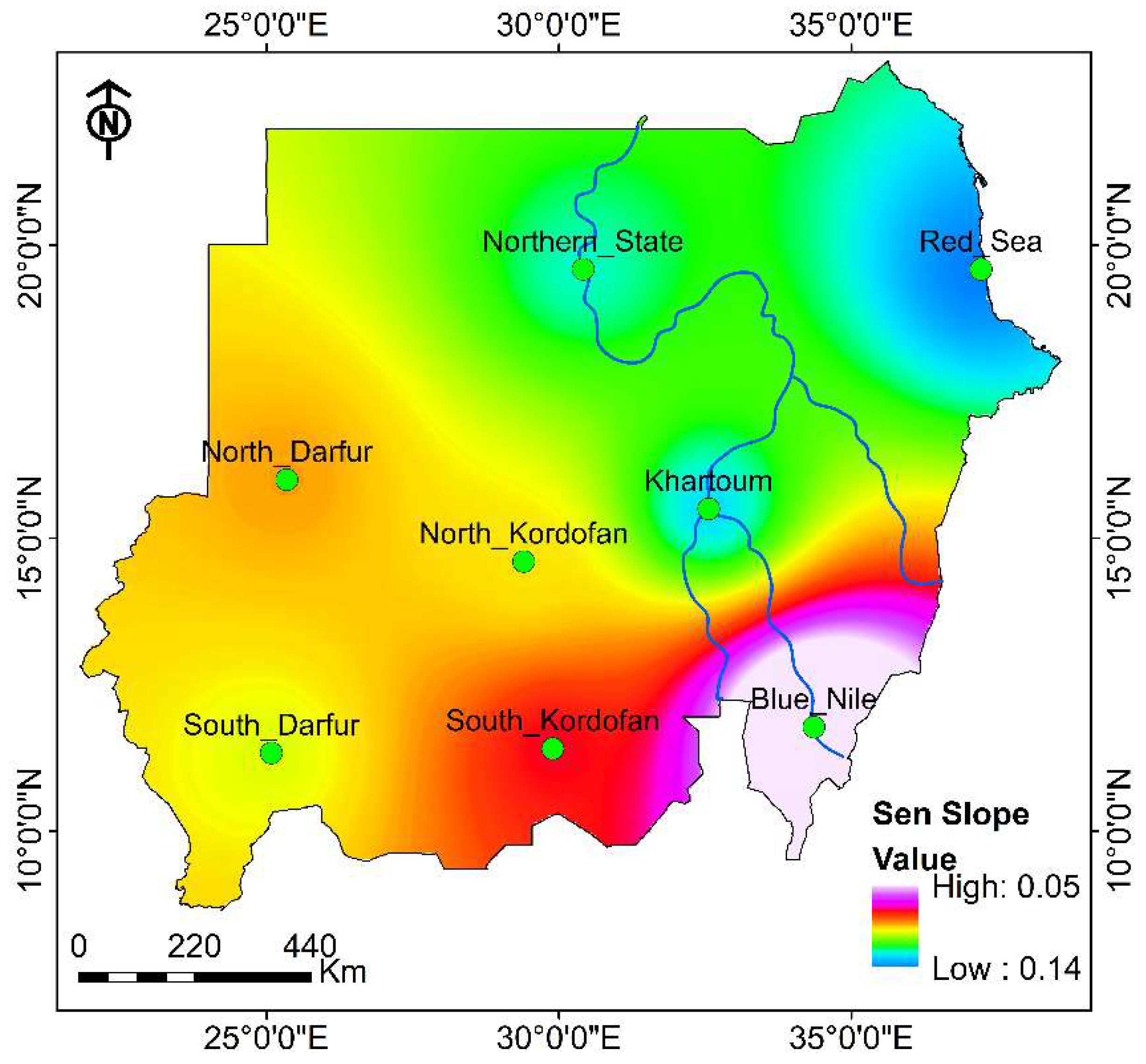
Sen’s slope estimator is used to quantify the magnitude of the detected trend [56], offering a robust and simple method to estimate the rate of change in the groundwater storage change. It calculates the slope between all pairs of data points in the dataset, defined as the change in value divided by the time interval. The Sen’s slope is then derived as the median of these individual slopes, providing a measure of the trend’s strength that is resistant to outliers and irregularities in the data. To evaluate the spatial distribution of water level trends Sen’s slope estimator was interpolated between monitoring stations using the inverse distance weighted method (IDW) [57].

4. Results and Discussion

4.1. Filling Gabs in TWS Anomalies

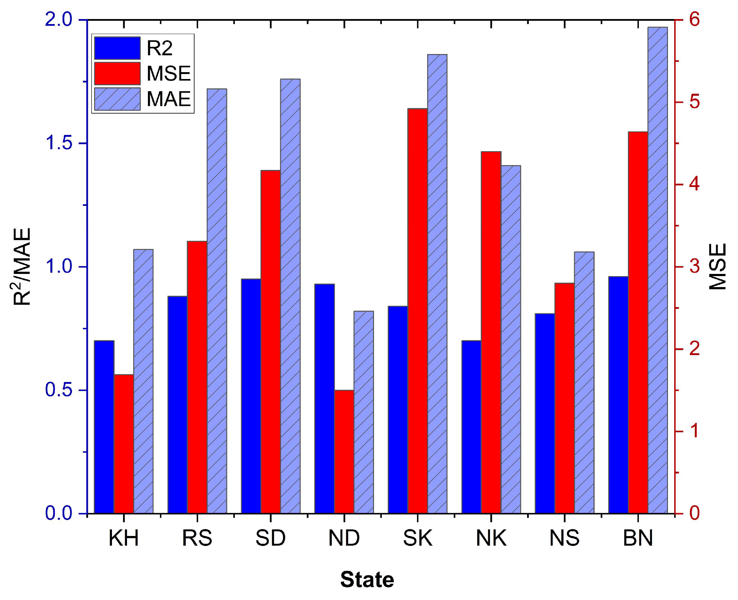
The GRACE TWS data used in this study cover April 2002 through January 2025, although intermittent gaps remain in the record. The Random Forest (RF) regression method described in Section 3.3 was applied to fill missing values in the original TWS anomaly time series. Two types of data gaps were considered: (i) the short 1–2-month gaps that occur periodically during the GRACE mission, and (ii) the longer consecutive gap between mid-2017 and mid-2018, when no GRACE observations were available. The RF model was trained using GLDAS parameters and temporal features of the observed TWS data. The model used 100 trees with a fixed random seed for consistency. Default settings were used for tree depth and node sizes, leveraging RF’s robustness to hyperparameter variation. To ensure that the RF gap-filling approach is robust, a mask-and-replace test we conducted where entire sections of the TWS record, including a full year, were deliberately removed and then reconstructed using the RF model. The reconstructed series was compared against the withheld observations. The model demonstrated robust performance across all stations in Sudan (Figure 4), with R2 values ranging from 0.70 to 0.96, indicating the model’s capacity to explain 70–96% of the variance in TWS time series. The observed mean square error (MSE) values (1.50–4.92 cm) and mean absolute error (MAE) values (0.82–1.97 cm) demonstrate hydrologically acceptable accuracy levels, particularly considering that GRACE-derived TWS anomalies exhibit high variations. This error magnitude is substantially lower than the natural variability of the system, indicating reliable model performance comparable to similar machine learning studies for TWS gap-filling [58].
The spatial variability in model performance reflects the diverse hydroclimatic conditions across Sudan’s different zones. The exceptional performance in the Blue Nile region (R2 = 0.96) can be attributed to the strong seasonal hydrological signal and well-defined precipitation patterns that characterize this area [30]. Studies have demonstrated that regions with pronounced seasonal cycles and consistent hydroclimatic patterns exhibit superior performance in GRACE-based TWS modeling [59]. The Blue Nile’s high TWS variability (~70 cm) provides sufficient signal strength for the RF algorithm to capture underlying patterns effectively, consistent with findings by Swenson and Wahr [60] who emphasized the importance of signal amplitude for GRACE accuracy. Similarly, the strong performance observed in South Darfur and North Darfur (R2 = 0.95 and 0.93, respectively) demonstrates the model’s robustness in arid and semi-arid environments. The reduced performance in Khartoum and North Kordofan (R2 = 0.70) can be attributed to several interconnected factors. Lower TWS amplitudes in these regions result in reduced signal-to-noise ratios, making pattern recognition more challenging [61]. Previous research in Sudanese hydrogeology has shown that central Sudan exhibits complex groundwater recharge patterns with rates, occurring primarily during heavy rainfall events [40], which may contribute to irregular TWS anomaly patterns that are more difficult to model.
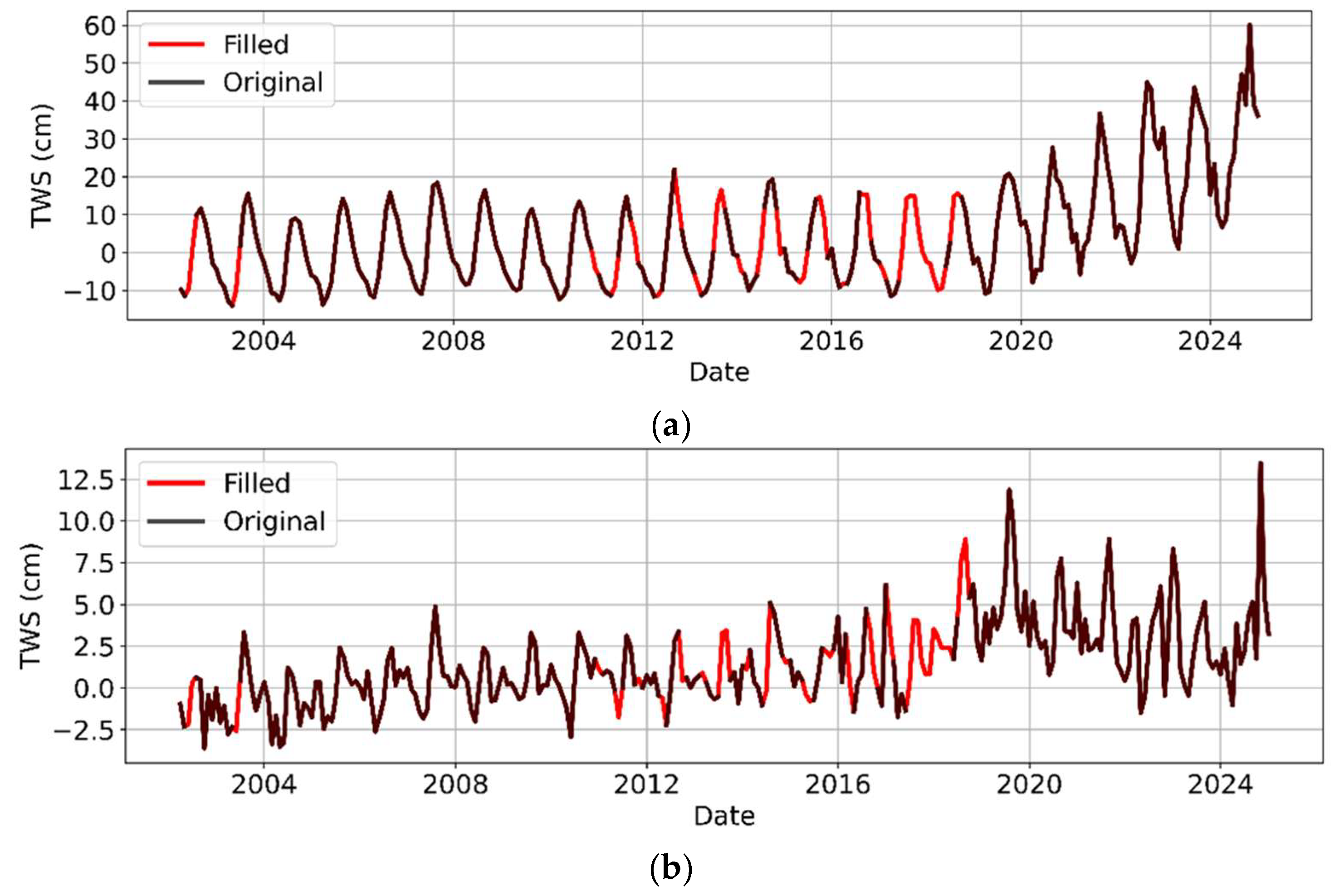
The RF approach offers several advantages for TWS gap-filling. The algorithm’s ability to handle nonlinear relationships and capture complex interactions between meteorological and hydrological variables makes it particularly suitable for diverse hydroclimatic conditions. Comparative studies have shown that RF models exhibit superior performance compared to multiple linear regression and artificial neural networks for TWS reconstruction at the basin scale [59]. While the Random Forest model demonstrates strong performance, the model is inherently dependent on the quality and amplitude of input data. Despite the regional variations, the overall model performance across all stations remained within acceptable error thresholds for hydrological applications. A visual inspection of the original and filled TWS time series for representative stations (Figure 5) confirms the validity of the quantitative results. The filled values closely follow the temporal evolution of the observed data without introducing spurious fluctuations or discontinuities. The model preserved key features such as seasonal cycles, interannual trends, and extreme anomaly events.

4.2. Groundwater Storage Change

The groundwater storage changes estimation relies on the water balance equation that relates TWS variations to the sum of individual storage components. Groundwater storage changes are calculated as the residual between GRACE-derived TWS changes and the sum of GLDAS-NOAH parameters converted to cm (GWS = TWS − [CWS + SMS + Qs]) across major Sudanese states from 2002 to 2025. To ensure consistency, all datasets were resampled to a common daily and monthly scale and aligned before computing groundwater storage anomalies. Agreement between the time series was checked prior to further analysis, confirming that deviations were minimized after temporal adjustment. Furthermore, the consistency was ensured by removing the same baseline mean from the GLDAS-derived components. In this way, both datasets are directly comparable.
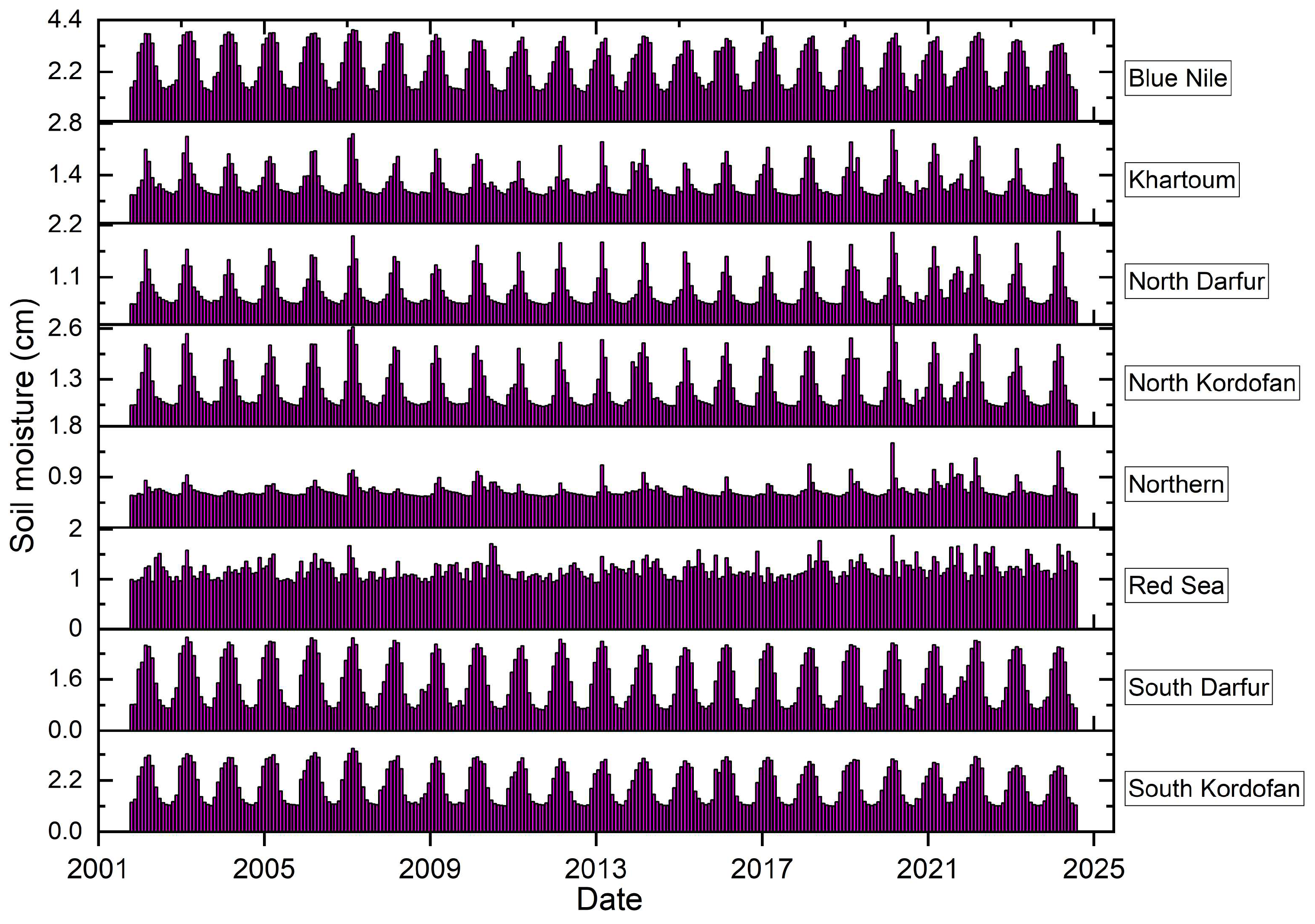
Surface soil moisture (SMS) exhibited marked spatiotemporal variability across all stations, reflecting Sudan’s pronounced climatic gradient. As expected, higher soil moisture levels were recorded in stations located in the southern and central parts of Sudan, such as Blue Nile and South Kordofan (Figure 6), where precipitation is more abundant and the climate is semi-humid [62]. In contrast, northern and central arid regions such as Northern, North Kordofan, North Darfur showed consistently lower SMS levels throughout the study period, generally with limited seasonal fluctuation. This pattern reflects the low rainfall and high evapotranspiration rates typical of desert and semi-desert climates [63]. Temporal trends in SMS indicate interannual variability, particularly during strong climate anomaly years, which correspond to periods of above-average rainfall in most parts of Sudan [64].
Surface runoff (Qs) values were generally low across most stations, with Qs values averaging below 0.0054 cm/month in arid and semi-arid areas such as North Darfur and Northern States. However, short-term spikes in runoff were observed in more humid regions like Blue Nile, Red Sea, and South Kordofan, particularly during 2007, 2010, and 2015, which likely correspond to localized heavy precipitation events and seasonal flooding [62]. The Blue Nile station exhibited the most prominent surface runoff events, which is consistent with its hydrological context within the Upper Nile Basin, where rainfall is more intense and runoff generation is facilitated by saturated soils and steep terrain. The limited runoff in northern stations underscores the infiltration-dominated hydrology and low precipitation rates, where most rainfall is quickly lost to infiltration and evaporation, and very little contributes to overland flow.
Canopy water storage (CWS) demonstrated the lowest values across all GLDAS parameters. The Blue Nile, South Darfur, and Red Sea stations showed relatively higher CWS compared to northern counterparts, indicating denser vegetation cover and higher precipitation frequency, which supports interception storage [46]. The CWS values were nearly zero in Northern, North Kordofan, and Khartoum, consistent with their sparse or absent vegetation cover typical of arid environments [63].
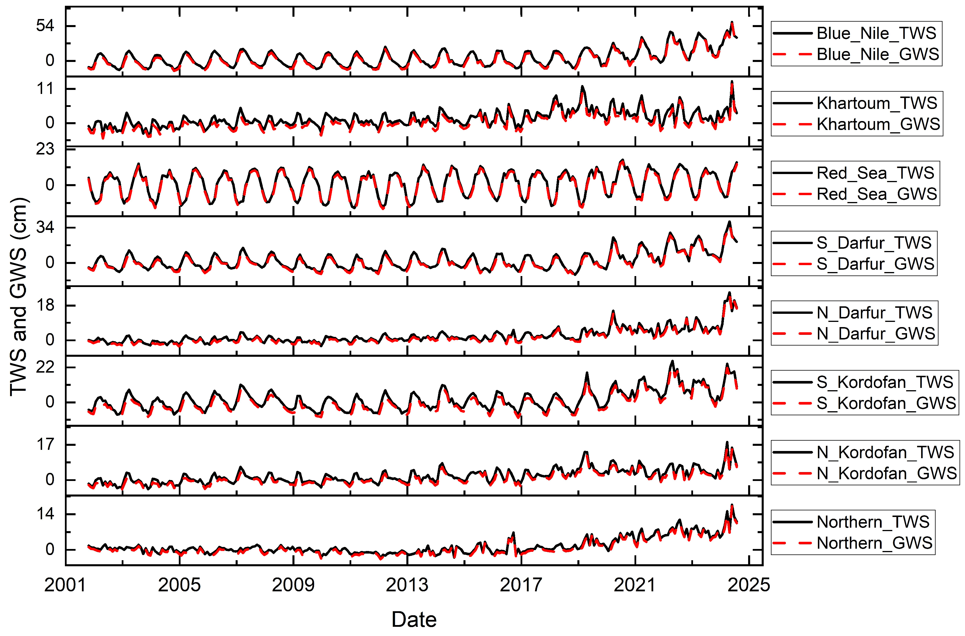
GWS generally exhibits parallelization with TWS trends (Figure 7). However, the magnitude of anomalies and the relationship between TWS and GWS differ spatially, reflecting diverse climatic and hydrogeological settings controlled by the underlying aquifer systems and their properties. The Blue Nile station stands out with consistently high GWS values. This region is underlain by alluvial and fluvial sediments consists of unconfined and unconsolidated aquifers, composed of alluvial sand, silt, clay, and gravel [65]. The high hydraulic conductivity of the alluvial aquifer (typically > 14 m/day) facilitates strong recharge from the adjacent Blue Nile River through direct infiltration and lateral groundwater flow [66]. This explains the sustained high storage levels that reflect continuous river–aquifer interaction, enhanced by seasonal flooding and relatively higher precipitation (600–800 mm/year) [35].
In Khartoum, located at the confluence of the Blue and White Nile, both TWS and GWS showed moderate anomalies compared to Blue Nile area. It is a densely urbanized area with high water demand, with the aquifer system benefits from the multi-layered Nubian Sandstone and Gezira formations with complementary hydraulic properties. The upper Gezira Formation provides moderate transmissivity (50–150 m2/day), while the deeper Nubian Sandstone offers substantial storage capacity with transmissivity values ranging from 100–500 m2/day [67]. A relatively wider gap between TWS and GWS in Khartoum is indicated which reflects the imbalance between recharge and extraction, likely driven by intensive groundwater abstraction.
Western Sudan (Kordofan and Darfur) exhibit consistent and moderately increasing TWS and GWS trends. These regions are characterized by distinct aquifer systems with contrasting properties. The Um Ruwaba Formation is unconsolidated and sometimes several hundred meters thick, but recharges very slowly from rainwater. North Kordofan is situated within the Umm Ruwaba Formation, which consists of extensive and thick unconsolidated sediments with moderate hydraulic properties. The water-resource potential properties of the main Umm Ruwaba aquifer are generally fair to good, with a shallow piezometric surface (<25 m deep) and favorable transmissivity [29]. South Kordofan overlies the Precambrian and Umm Ruwaba aquifer systems [68]. Groundwater occurs primarily in both sedimentary and weathered and fractured zones with lower but sustainable yields making the groundwater storage higher than that of north. The relatively close alignment between TWS and GWS indicates that groundwater dominates the total storage signal and that recharge processes are sufficient to support current usage levels. The Darfur stations (North and South) also show positive storage trends but with slightly greater temporal variability. The subsurface geology is largely dominated by the Nubian Aquifer, with basement exposures in the south.
In the Red Sea region, despite the predominance of thin alluvial aquifer and low-porosity Precambrian basement rocks, storage values are unexpectedly positive. This suggests the presence of effective localized recharge mechanisms, such as runoff concentration along wadis and preferential recharge through fractured rock zones and weathered profiles, particularly during sporadic rainfall events [35]. The alluvial and fractured basement aquifers exhibit low but variable transmissivity and specific capacity [69]. The relatively close TWS–GWS alignment indicates limited but stable aquifer response to such recharge events. The Northern State station, located in the hyper-arid Nubian Desert, consistently exhibits the lowest TWS and GWS values. Despite the low precipitation, the underlying Nubian Sandstone Aquifer has immense storage capacity. The close similarity between TWS and GWS signals confirms that groundwater dominates the water storage component, and limited surface water in this desert region. The positive storage trends likely reflect artesian pressure responses and very slow drainage from the vast aquifer system rather than active recharge, indicating that current abstraction represents mining of fossil groundwater resources.
The results of the trend analysis using Sen’s slope estimation revealed statistically significant long-term trends in both TWS and GWS across all stations (Table 1). The estimated Sen’s slopes indicate positive trends at all sites, with values ranging from approximately 0.016–0.068 cm across the study period. The strongest increasing trends are observed in the Blue Nile region, where both TWS (0.068 cm/year) and GWS (0.068 cm/year) show the highest slope values. Similarly, Southern Kordofan and Southern Darfur display relatively high positive slopes (~0.035 cm/year), reflecting consistent storage gains in these regions. In contrast, stations such as Red Sea and Northern Sudan exhibit comparatively lower slope values (~0.016–0.019 cm/year), but the trends remain statistically significant. These findings collectively indicate that, over the study period, Sudan has generally experienced a gradual increase in both TWS and GWS, with spatial variability reflecting differences in climate conditions, recharge mechanisms, and groundwater abstraction pressures across the different hydroclimatic zones.
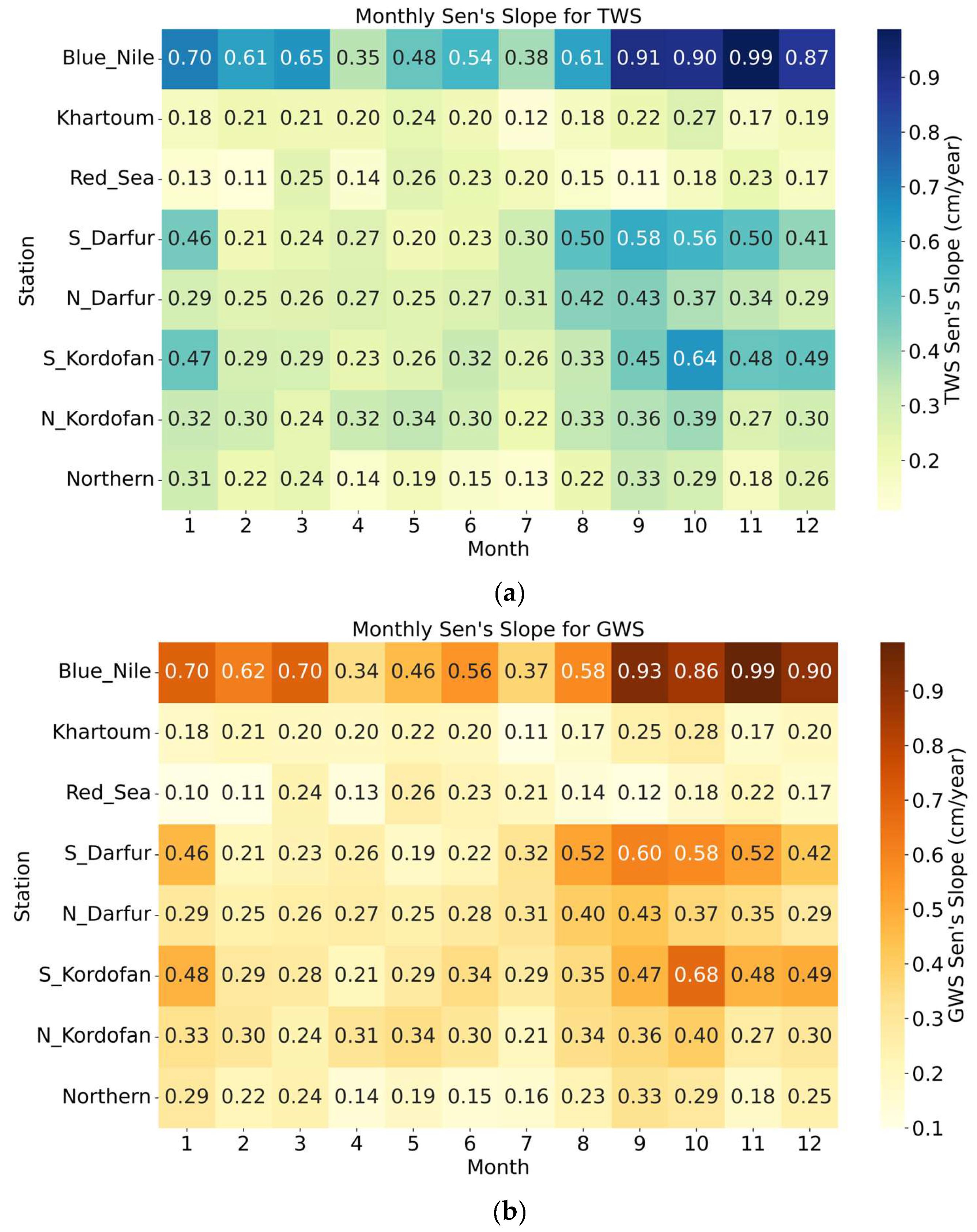
To evaluate the seasonal trends of TWS and GWS across Sudan, the Sen’s slope was calculated for each month of the year for all stations. For each month (January to December), the corresponding monthly values over the years were used to compute the slope, providing estimate of the annual rate of change in cm/year (Figure 8). This approach captures seasonal variations by producing a slope for each month separately, rather than a single slope for the entire time series. The monthly Sen’s slope analysis highlights clear seasonal variations in both TWS (Figure 8a) and GWS (Figure 8b) across Sudan. The Blue Nile station exhibits the most pronounced variability, with GWS trends ranging from 0.35 cm/yr in April to a peak of 0.99 cm/yr in November. TWS at this station shows a similar seasonal amplitude, with the sharpest declines during the autumn months (September–November). In Darfur, South Darfur records notable autumn peaks (up to 0.60 cm/yr for GWS and 0.58 cm/yr for TWS in September), whereas North Darfur maintains more stable trends (0.25–0.43 cm/yr), reflecting contrasting hydrogeological responses within the same region. The Kordofan stations also show distinct contrasts: South Kordofan experiences clear October peaks in both GWS (0.68 cm/yr) and TWS (0.64 cm/yr), while North Kordofan remains relatively uniform throughout the year, suggesting different levels of climatic influence on subsurface dynamics. In contrast, Khartoum, the Red Sea, and Northern stations display consistently low Sen’s slopes (0.10–0.28 cm/yr), indicating relatively stable conditions with limited seasonal fluctuation.

4.3. Decomposition and Prediction of GWS

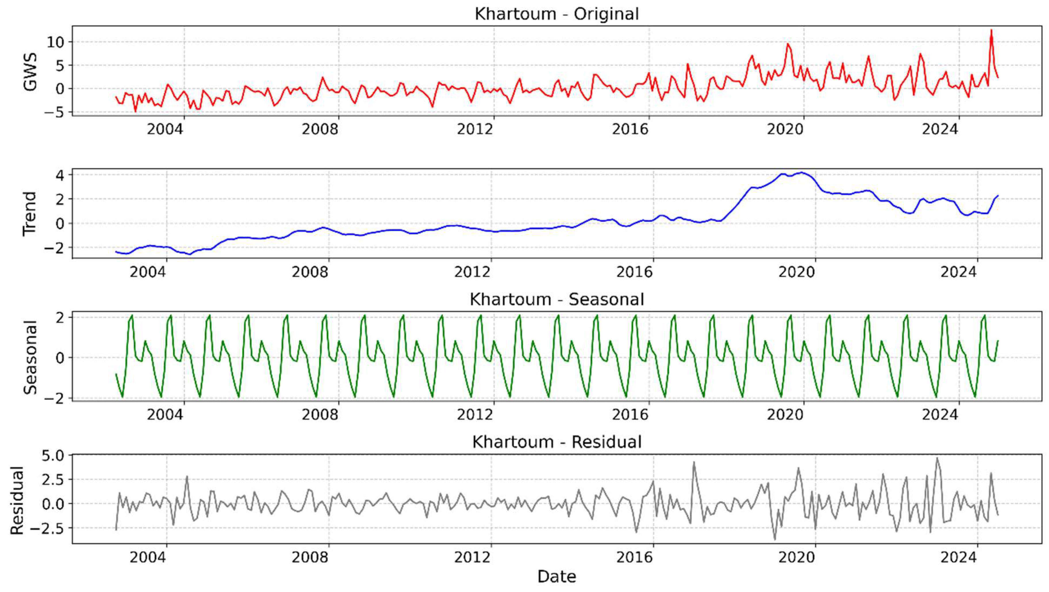
Groundwater storage (GWS) change forecasting was carried out using the gap-filled time series data as the primary input. The aim was to project groundwater dynamics beyond the observational record while also quantifying the uncertainty of these projections. To separate long-term changes from short-term variability, the GWS series was decomposed into three components including trend, seasonal, and residual, using seasonal-trend decomposition (STL). This step ensured that the model could focus on the systematic trend in groundwater storage without being confounded by predictable seasonal cycles or random fluctuations driven by short-term climatic events. An example of this decomposition is shown in Figure 9, where the long-term trend is clearly separated from seasonal and residual variability. Following this step, a bootstrapped BiLSTM ensemble was trained specifically on the extracted trend component of the GWS series. This allows us to capture temporal dependencies in the long term. Thus, the forecasts were based solely on the GRACE/GRACE-FO groundwater anomaly recorded after reconstruction and decomposition where the time features (year, month, day) are used as an input (Predictor) and the GWS as output.
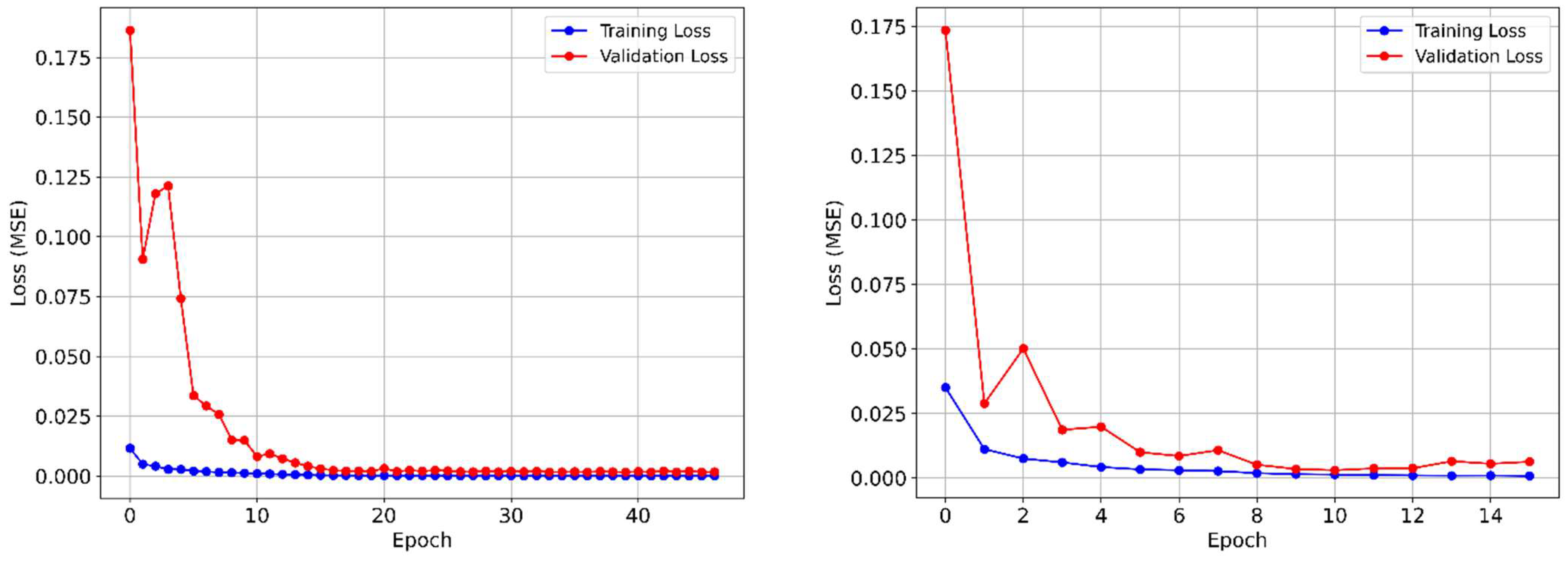
The architecture and training hyperparameters of the model were optimized using a combination of random search and experimental tuning within predefined parameter ranges. A number of 50 bootstraps were employed, wherein the training data were resampled, and each resample was used to train an independent Bi-LSTM model. The number of LSTM units varied between 32 and 256, while the size of the hidden dense layer ranged from 16 to 128 neurons. Learning rates were explored within the interval of 0.00001 to 0.001, and batch sizes from 16 to 64 were tested. The final optimized model configuration consisted of a Bi-LSTM layer with 150 units, followed by a dense layer with 75 neurons and a single output node. To prevent overfitting, early stopping was applied during training, and its effectiveness is reflected in the loss curves across all eight stations. As shown in the representative loss curve (Figure 10), both training and validation losses exhibited a steep decline within the first 2–10 epochs, with validation loss stabilizing shortly thereafter. The early stopping mechanism successfully halted training once validation loss plateaued, resulting in efficient training durations. For most stations, convergence occurred between 30 and 40 epochs, while more complex groundwater signal patterns required up to 50 epochs. The close alignment of training and validation losses at minimal values across all stations confirms strong model generalization and absence of overfitting.
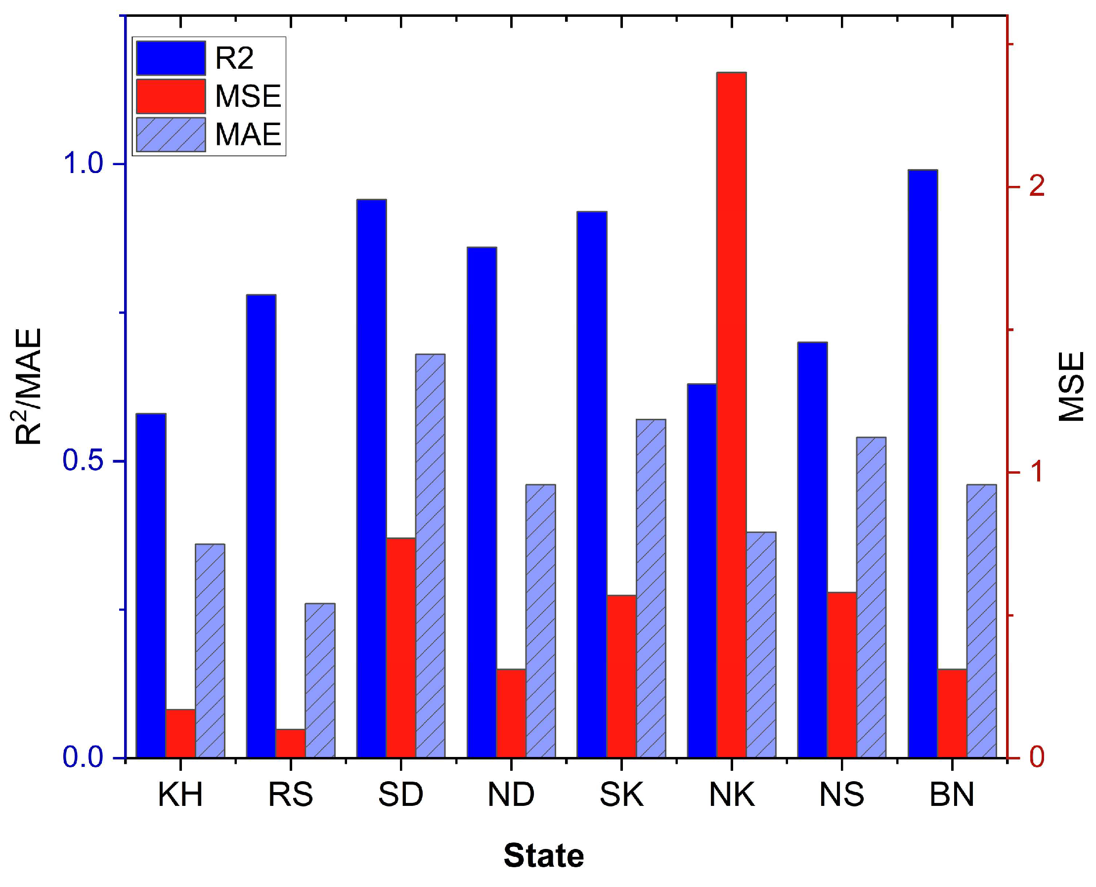
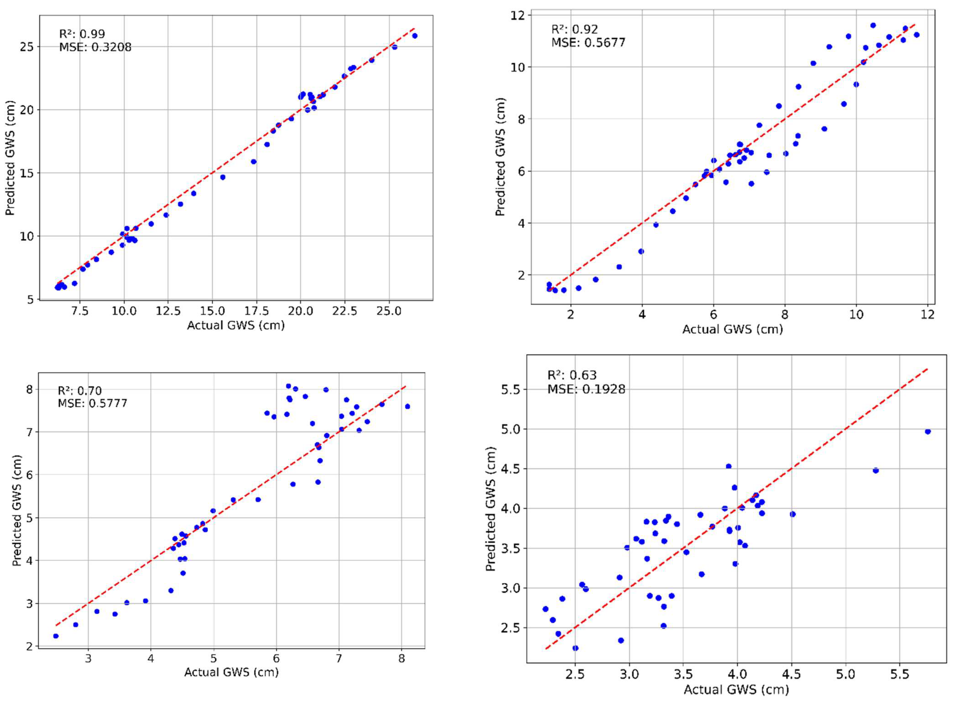
The bootstrapped LSTM model demonstrated varying levels of predictive accuracy across the studied states (Figure 11), reflecting differences in groundwater system dynamics and signal complexity. Among all regions, Blue Nile and South Darfur showed the highest predictive accuracy, with R2 values of 0.99 and 0.94, respectively (Figure 12). These high coefficients of determination indicate that the model effectively captured the long-term groundwater storage trends in these areas. The model’s success in these regions can be attributed to their relatively stable, monotonic trends despite the large magnitude changes. Additionally, their corresponding RMSE and MAE values were relatively low, particularly in South Darfur (RMSE = 0.77, MAE = 0.68), suggesting consistent predictions. South Kordofan and North Darfur also exhibited strong model performance, with R2 values of 0.92 and 0.86, respectively (Figure 12), and moderate error levels. In contrast, Khartoum and North Kordofan showed comparatively lower predictive performance, with R2 values of 0.58 and 0.63, respectively. Khartoum’s complex signal variability, transitioning from declining to recovering trends with multiple fluctuations, likely contributed to the modeling challenges. Notably, North Kordofan presented an anomalously high RMSE of 2.4, which corresponds to its highly volatile GWS pattern, experiencing the most dramatic recovery among all stations. Red Sea and Northern State achieved moderate accuracy, with R2 values of 0.78 and 0.70, respectively, and relatively balanced errors. These results suggest that while the model can adequately generalize across different hydroclimatic zones, its performance is enhanced in regions where the groundwater trend exhibits more stable temporal patterns and less seasonal or irregular noise.

4.4. Forecasting and Uncertainty Analysis

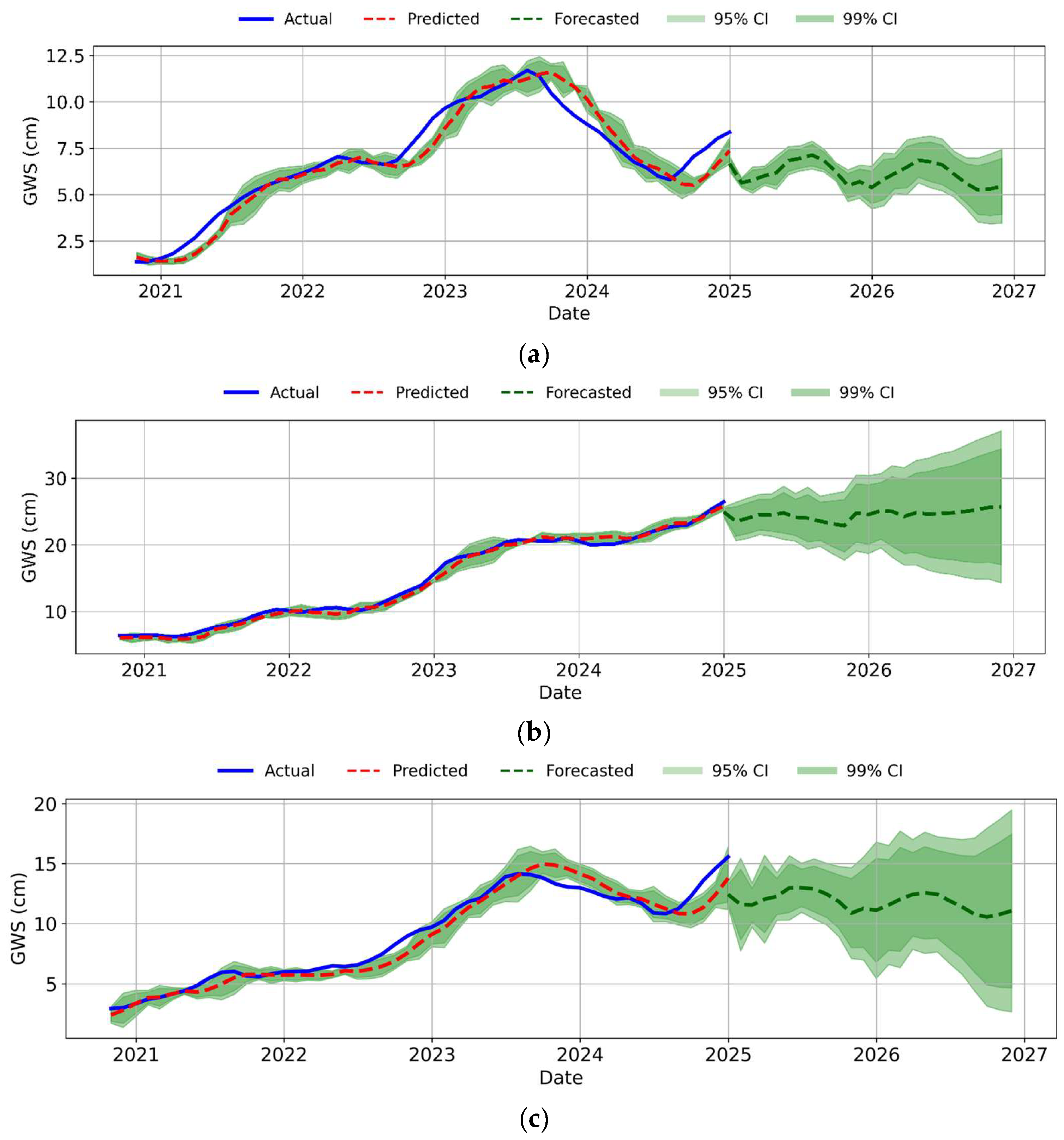
The forecasting of GWS is further performed using the bootstrapped BiLSTM model. This ensemble modeling captured model and data uncertainties and produced confidence intervals (CIs) around the predictions and forecasts. The 95% and 99% prediction intervals revealed significant differences in uncertainty levels among regions (Figure 13). The Blue Nile station demonstrates exceptional forecasting confidence with remarkably narrow confidence intervals throughout the prediction period. The central forecast trajectory projects continued positive growth, reaching approximately +25 cm by 2027, maintaining the established upward trend observed in historical data. The 95% confidence intervals range from ±0.5 cm to ±8 cm, widening progressively with increasing forecast lead time due to the inherent rise in uncertainty over longer prediction horizons. Narrow intervals at shorter lead times indicate highly predictable groundwater behavior, driven by stable hydrological processes. This high confidence is supported by the station’s consistent historical performance and well-defined seasonal and interannual patterns in the observed data.
Khartoum exhibits moderate to low forecasting confidence with the central prediction maintaining stable levels around 1 cm throughout 2025–2027. The CIs are broader than Blue Nile considering the amplitude of the GWS, with 95% intervals extending to ±1 cm. The moderate confidence reflects the complex urban hydrogeological setting where multiple factors influence GWS dynamics, including groundwater abstraction and multi-aquifer interactions. The broader CIs acknowledge the increased uncertainty inherent in forecasting system with multiple competing influences, though the overall stability of the forecast trajectory suggests the model has captured the fundamental water balance dynamics. The Red Sea station exhibits the narrow CIs among all monitoring points, with 95% intervals spanning ±0.5–1.3 cm. The central forecast maintains positive reaching 2 cm by 2027 but shows considerable uncertainty in the low GWS values. The lower CIs is entirely justified given the irregular behavior of the GWS in this part of Sudan. The broad confidence intervals appropriately reflect the limited predictability in such heterogeneous system. Northern State shows moderate to high confidence with relatively narrow and consistent intervals for the magnitude of changes predicted. The central forecast suggests minimal growth, reaching 8.2 by 2027, with 95% CIs of ±1.7 cm. The consistent confidence reflects the Nubian Sandstone’s large-scale storage characteristics and minimal active recharge in hyperarid conditions. While the absolute changes are small, the model demonstrates good confidence in predicting the subtle pressure responses and slow drainage dynamics characteristic of water systems.
North Darfur shows high in the CIs with the central forecast reaching approximately 8 cm by 2027. However, the confidence intervals display notable variability, with 95% CIs ranging from ±1.5−3 cm depending on the forecast period. The prediction exhibits some seasonal oscillations superimposed on the overall positive trend However, a decline is noticed by the end of 2026. The broader intervals during certain forecast periods acknowledge the model’s recognition of increased uncertainty. South Darfur, on the other hand, demonstrated consistent CIs throughout the prediction and forecast periods, with progressive increse. The central forecats showing steady growth to approximately 11.5 cm by 2027. The 95% CIs maintain relatively stable widths of ± 1–6.5 cm. The consistent CIs levels reflect the station’s more predictable hydrological behavior compared to North Darfur, despite sharing almost similar geological settings. This suggests that local variations in climate patterns and land use create more stable GWS dynamics in the South Darfur region. South Kordofan exhibits some of the highest forecasting confidence among all stations, with narrow confidence intervals and clear upward trajectory reaching 5.5 cm by 2027. The 95% confidence intervals remain within ± 0.1–3.5 cm throughout the forecast period, demonstrating exceptional model reliability. North Kordofan shows low forecasting performance with central predictions reaching approximately 3 cm by 2027. The CIs display high width with 95% intervals reachs maximum of ±6 cm. This wide spread highlights substantial uncertainty, likely driven by irregular recharge patterns and greater temporal variability in the groundwater dynamics.
The use of the bootstrapped BiLSTM model demonstrated good generalization capabilities across different diverse hydroclimatic zones, with particularly high performance in regions where groundwater trends exhibited stable temporal patterns and minimal seasonal or irregular fluctuations. This outcome aligns with findings from previous studies, which highlight that deep learning models, especially LSTM-based architectures, tend to perform better when the underlying hydrological signals are less affected by high-frequency noise or abrupt anomalies [70,71]. In the present study, the initial seasonal-trend decomposition played a crucial role in reducing noise and isolating the long-term trend component, thereby enhancing the model’s predictive accuracy. Similar preprocessing approaches have been shown to improve hydrological forecasting by allowing models to focus on persistent signals rather than transient variability [72]. Nevertheless, certain stations still exhibited only moderate prediction and forecasting performance, likely due to the combined influence of high climatic variability, irregular recharge events, and anthropogenic pressures such as intensive groundwater abstraction. Previous works have reported comparable challenges, noting that deep learning models can struggle in data-scarce [21] or highly variable systems where external drivers exert strong and unpredictable impacts on groundwater dynamics. It is important to note that forecasting inherently involves uncertainty, particularly when extending beyond the observed record. As a result, the model may not fully align with the last available observations at the end of the prdiction period. This limitation can manifest as a small mismatch between predicted and actual values at the transition point, as observed in the final steps of the series. Such deviations occur because probabilistic forecasting generates independent generalized trajectories rather than reproducing the last observed point exactly. Nonetheless, the model demonstrates high overall performance across the validation periods, capturing broader temporal trends and providing useful forecasts despite the expected short-term discrepancies.

4.5. Trend Analysis of the Forecasted GWS Anomalies

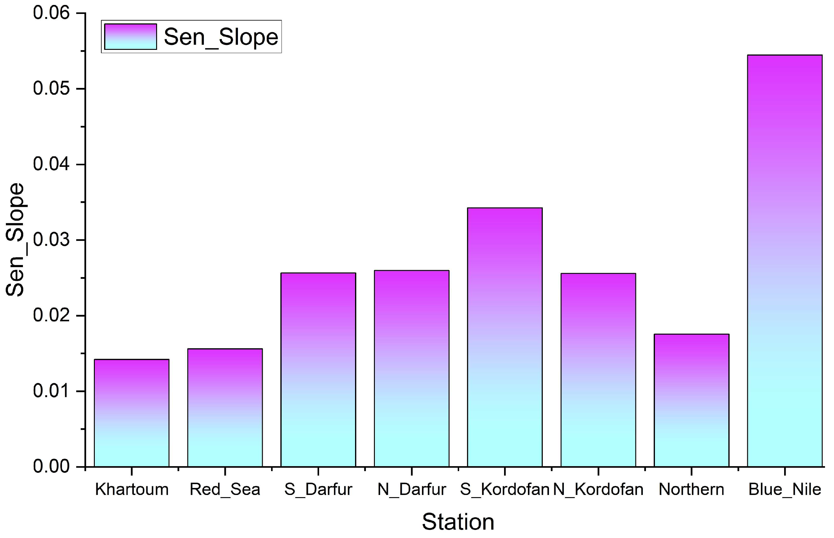
The trend analysis of the forecasted GWS shows consistently positive and increasing patterns across all eight stations, though with varying magnitudes (Figure 14). The strongest trend was observed in the Blue Nile region, followed by South Kordofan, and both North and South Darfur, reflecting steady aquifer recovery in these areas. Moderate trends were recorded in North Kordofan, Northern State, and Khartoum, while the Red Sea station showed the lowest rate of increase. The spatial trend map (Figure 14) were produced using the long-term trends of the combined historical and forecasted groundwater storage at each analysis station. These point-based trend estimates were interpolated using Inverse Distance Weighting (IDW) to create a continuous surface and highlight the regional variability in groundwater storage trends across Sudan. The spatial trend analysis reveals a clear geographic gradient in GWS recovery across Sudan (Figure 15), shaped by the interplay of climate, geology, and aquifer properties. Southern and southwestern regions exhibit the highest recovery rates, driven by abundant rainfall and highly permeable aquifers like Um Ruwaba formations, which facilitate recharge from seasonal floods and precipitation. Central regions show moderate recovery, supported by multi-aquifer systems with buffering capacity and mixed recharge mechanisms. In contrast, northern and eastern regions, characterized by arid climates and low recharge potential, display limited but still positive trends, reflecting deep storage dynamics. These trends underscore the importance of aligning groundwater management strategies with regional hydrogeological conditions. While southern systems may support more active use, northern aquifers require cautious management to sustain storage. The findings highlight the critical need for region-specific groundwater policies informed by climate-aquifer interactions and long-term storage behavior.

5. Conclusions

This study presents an integrated framework that combines satellite-based GRACE observations with machine learning techniques to investigate and forecast GWS dynamics across Sudan. Random Forest (RF) regression filled the gaps in GRACE-derived TWS data, while a bootstrapped BiLSTM model predicted the groundwater storage trends and quantified forecast uncertainty. The RF successfully addressed data gaps, enabling complete temporal coverage for forecasting. The BiLSTM model achieved strong predictive performance, with R2 values ranging from 0.58 to 0.99 across stations, reflecting adaptability to varying hydrogeological conditions. The analysis reveals consistent and statistically significant positive GWS trends across all eight study regions. Spatially, higher recovery rates were observed in southern and southwestern regions, tapering off toward the north and east which is linked to climatic gradients and groundwater recharge potential. The clear spatial gradient in recovery emphasizes the need for regionally tailored management strategies. The probabilistic nature of the forecasting framework enables risk-informed planning, allowing stakeholders to weigh confidence levels in future scenarios when developing policy or allocating resources.
The approach demonstrates the utility of GRACE and machine learning in data-scarce contexts, with potential for broader application in similarly under-monitored regions. However, the coarse spatial resolution of GRACE may obscure local variations, and its limited temporal span constrains long-term trend evaluation. The decomposition-focused forecasting emphasizes trends but may underrepresent short-term anomalies or extreme events. The absence of ground-based validation data limits assessment of absolute GWS values. Future work could focus on integrating the forecasted GWS trends with a groundwater flow model to assess the impact of different extraction scenarios on aquifer sustainability. Exploring hybrid models that blend machine learning with physically based simulations could enhance interpretability and accuracy. Scenario-based forecasting under various climate and water-use projections will be crucial for long-term planning.

Supplementary Materials

The following supporting information can be downloaded at: https://www.mdpi.com/article/10.3390/rs17183172/s1, Figure S1: Forecasting results, Table S1: Hyper Parameters of the BiLSTM model used for forecasting groundwater storage change.

Author Contributions

Conceptualization, M.A.A.M. and P.S.; methodology, M.A.A.M. and J.O.A.; software, M.A.A.M.; validation, N.P.S. and P.S.; formal analysis; data curation, J.O.A.; writing—original draft preparation, M.A.A.M.; writing—review and editing, J.O.A., N.P.S. and P.S.; supervision, P.S. and N.P.S.; project administration, P.S.; funding acquisition, P.S. All authors have read and agreed to the published version of the manuscript.

Funding

The research was funded by the Sustainable Development and Technologies National Program of the Hungarian Academy of Sciences (FFT NP FTA).

Acknowledgments

The authors thank the Sustainable Development and Technologies National Program of the Hungarian Academy of Sciences (FFT NP FTA).

Conflicts of Interest

The authors declare no conflicts of interest.

References

  1. Frappart, F.; Ramillien, G. Monitoring Groundwater Storage Changes Using the Gravity Recovery and Climate Experiment (GRACE) Satellite Mission: A Review. Remote Sens. 2018, 10, 829. [Google Scholar] [CrossRef]
  2. Masood, A.; Tariq, M.A.U.R.; Hashmi, M.Z.U.R.; Waseem, M.; Sarwar, M.K.; Ali, W.; Farooq, R.; Almazroui, M.; Ng, A.W.M. An Overview of Groundwater Monitoring through Point-to Satellite-Based Techniques. Water 2022, 14, 565. [Google Scholar] [CrossRef]
  3. Ali, S.; Liu, D.; Fu, Q.; Cheema, M.J.M.; Pham, Q.B.; Rahaman, M.M.; Dang, T.D.; Anh, D.T. Improving the Resolution of GRACE Data for Spatio-Temporal Groundwater Storage Assessment. Remote Sens. 2021, 13, 3513. [Google Scholar] [CrossRef]
  4. Rateb, A.; Scanlon, B.R.; Pool, D.R.; Sun, A.; Zhang, Z.; Chen, J.; Clark, B.; Faunt, C.C.; Haugh, C.J.; Hill, M.; et al. Comparison of Groundwater Storage Changes from GRACE Satellites with Monitoring and Modeling of Major US Aquifers. Water Resour. Res. 2020, 56, e2020WR027556. [Google Scholar] [CrossRef]
  5. Yidana, S.M.; Dzikunoo, E.A.; Mejida, R.A.; Ackom, E.K.; Chegbeleh, L.P.; Loh, Y.S.A.; Banoeng-Yakubo, B.K.; Akabzaa, T.M. Evaluating Groundwater Resources Trends through Multiple Conceptual Models and GRACE Satellite Data. Environ. Monit. Assess. 2024, 196, 290. [Google Scholar] [CrossRef] [PubMed]
  6. Ding, K.; Zhao, X.; Cheng, J.; Yu, Y.; Luo, Y.; Couchot, J.; Zheng, K.; Lin, Y.; Wang, Y. GRACE/ML-Based Analysis of the Spatiotemporal Variations of Groundwater Storage in Africa. J. Hydrol. 2025, 647, 132336. [Google Scholar] [CrossRef]
  7. Mohasseb, H.A.; Shen, W.; Jiao, J.; Hassan, A.A. Estimation of Groundwater Storage Variations in African River Basins: Response to Global Climate Change Using GRACE and GRACE-FO among Past Two Decades. Adv. Space Res. 2024, 74, 1164–1182. [Google Scholar] [CrossRef]
  8. Mohamed, A.; Alarifi, S.S.; Al-Kahtany, K.; Mohammed, M.A.A. Application of Gravity and Remote Sensing Data to Groundwater Storage Variation in Wadi Al Dawasir, Saudi Arabia. J. King Saud. Univ. Sci. 2024, 36, 103172. [Google Scholar] [CrossRef]
  9. Mohamed, A.; Alarifi, S.S.; Mohammed, M.A.A. Geophysical Monitoring of the Groundwater Resources in the Southern Arabian Peninsula Using Satellite Gravity Data. Alex. Eng. J. 2024, 86, 311–326. [Google Scholar] [CrossRef]
  10. Nikraftar, Z.; Parizi, E.; Saber, M.; Hosseini, S.M.; Ataie-Ashtiani, B.; Simmons, C.T. Groundwater Sustainability Assessment in the Middle East Using GRACE/GRACE-FO Data. Hydrogeol. J. 2024, 32, 321–337. [Google Scholar] [CrossRef]
  11. Upadhyay, S.; Shrestha, S.; Loc, H.H.; Mohanasundaram, S.; Dhungana, S.; Lim, S.; Tangdamrongsub, N. Satellite-Based Estimates of Declining Groundwater Storage in the Transboundary Cambodia-Mekong River Delta Aquifer of the Lower Mekong Region, Southeast Asia. Hydrogeol. J. 2024, 32, 601–619. [Google Scholar] [CrossRef]
  12. Dharpure, J.K.; Howat, I.M.; Kaushik, S. Declining Groundwater Storage in the Indus Basin Revealed Using GRACE and GRACE-FO Data. Water Resour. Res. 2025, 61, e2024WR038279. [Google Scholar] [CrossRef]
  13. Li, W.; Bao, L.; Yao, G.; Wang, F.; Guo, Q.; Zhu, J.; Zhu, J.; Wang, Z.; Bi, J.; Zhu, C.; et al. The Analysis on Groundwater Storage Variations from GRACE/GRACE-FO in Recent 20 Years Driven by Influencing Factors and Prediction in Shandong Province, China. Sci. Rep. 2024, 14, 5819. [Google Scholar] [CrossRef] [PubMed]
  14. Nourani, V.; Paknezhad, N.J.; Ng, A.; Wen, Z.; Dabrowska, D.; Üzelaltınbulat, S. Application of the Machine Learning Methods for GRACE Data Based Groundwater Modeling, a Systematic Review. Groundw. Sustain. Dev. 2024, 25, 101113. [Google Scholar] [CrossRef]
  15. Wang, L.; Zhang, Y. Filling GRACE Data Gap Using an Innovative Transformer-Based Deep Learning Approach. Remote Sens. Environ. 2024, 315, 114465. [Google Scholar] [CrossRef]
  16. Chen, J.; Wang, L.; Chen, C.; Peng, Z. Downscaling and Gap-Filling GRACE-Based Terrestrial Water Storage Anomalies in the Qinghai–Tibet Plateau Using Deep Learning and Multi-Source Data. Remote Sens. 2025, 17, 1333. [Google Scholar] [CrossRef]
  17. Yin, W.; Zhang, G.; Liu, F.; Zhang, D.; Zhang, X.; Chen, S. Improving the Spatial Resolution of GRACE-Based Groundwater Storage Estimates Using a Machine Learning Algorithm and Hydrological Model. Hydrogeol. J. 2022, 30, 947–963. [Google Scholar] [CrossRef]
  18. Kashani, A.; Safavi, H.R. Assessing Groundwater Drought in Iran Using GRACE Data and Machine Learning. Sci. Rep. 2025, 15, 14671. [Google Scholar] [CrossRef]
  19. Satizábal-Alarcón, D.A.; Suhogusoff, A.; Ferrari, L.C. Characterization of Groundwater Storage Changes in the Amazon River Basin Based on Downscaling of GRACE/GRACE-FO Data with Machine Learning Models. Sci. Total Environ. 2024, 912, 168958. [Google Scholar] [CrossRef]
  20. Malakar, P.; Mukherjee, A.; Bhanja, S.N.; Ray, R.K.; Sarkar, S.; Zahid, A. Machine-Learning-Based Regional-Scale Groundwater Level Prediction Using GRACE. Hydrogeol. J. 2021, 29, 1027–1042. [Google Scholar] [CrossRef]
  21. Moudgil, P.S.; Rao, G.S. Groundwater Levels Estimation from GRACE/GRACE-FO and Hydro-Meteorological Data Using Deep Learning in Ganga River Basin, India. Environ. Earth Sci. 2023, 82, 441. [Google Scholar] [CrossRef]
  22. Mohammed, M.A.A.; Szabó, N.P.; Szűcs, P. Exploring Spatiotemporal Groundwater Flow Patterns in Heterogeneous Systems: A Comprehensive Workflow Combining Multiple Machine Learning Models. Stoch. Environ. Res. Risk Assess. 2025, 1–20. [Google Scholar] [CrossRef]
  23. Samani, S.; Vadiati, M.; Kisi, O. Predicting Groundwater Levels in Coastal Aquifers Using Deep Learning Models: A Comparative Study of Sedimentary and Metamorphic Aquifers in Nova Scotia. Earth Sci. Inform. 2025, 18, 389. [Google Scholar] [CrossRef]
  24. Aderemi, B.A.; Olwal, T.O.; Ndambuki, J.M.; Rwanga, S.S. Groundwater Levels Forecasting Using Machine Learning Models: A Case Study of the Groundwater Region 10 at Karst Belt, South Africa. Syst. Soft Comput. 2023, 5, 200049. [Google Scholar] [CrossRef]
  25. Guo, F.; Li, S.; Zhao, G.; Hu, H.; Zhang, Z.; Yue, S.; Zhang, H.; Xu, Y. A SOM-LSTM Combined Model for Groundwater Level Prediction in Karst Critical Zone Aquifers Considering Connectivity Characteristics. Environ. Earth Sci. 2024, 83, 267. [Google Scholar] [CrossRef]
  26. Yin, W.; Fan, Z.; Tangdamrongsub, N.; Hu, L.; Zhang, M. Comparison of Physical and Data-Driven Models to Forecast Groundwater Level Changes with the Inclusion of GRACE—A Case Study over the State of Victoria, Australia. J. Hydrol. 2021, 602, 126735. [Google Scholar] [CrossRef]
  27. Gaffoor, Z.; Pietersen, K.; Jovanovic, N.; Bagula, A.; Kanyerere, T.; Ajayi, O.; Wanangwa, G. A Comparison of Ensemble and Deep Learning Algorithms to Model Groundwater Levels in a Data-Scarce Aquifer of Southern Africa. Hydrology 2022, 9, 125. [Google Scholar] [CrossRef]
  28. Anderson, M.P.; Woessner, W.W.; Hunt, R.J. Applied Groundwater Modeling: Simulation of Flow and Advective Transport; Academic Press: Cambridge, MA, USA, 2015. [Google Scholar]
  29. Omer, A. Focus on Groundwater in Sudan. Environ. Geol. 2002, 41, 972–976. [Google Scholar] [CrossRef]
  30. Mohamed, A.; Sultan, M.; Ahmed, M.; Yan, E.; Ahmed, E. Aquifer Recharge, Depletion, and Connectivity: Inferences from GRACE, Land Surface Models, and Geochemical and Geophysical Data. GSA Bull. 2017, 129, 534–546. [Google Scholar] [CrossRef]
  31. Bonsor, H.C.; Mansour, M.M.; MacDonald, A.M.; Hughes, A.G.; Hipkin, R.G.; Bedada, T. Interpretation of GRACE Data of the Nile Basin Using a Groundwater Recharge Model. Hydrol. Earth Syst. Sci. 2010, 7, 4501–4533. [Google Scholar]
  32. Abdelmohsen, K.; Sultan, M.; Ahmed, M.; Save, H.; Elkaliouby, B.; Emil, M.; Yan, E.; Abotalib, A.Z.; Krishnamurthy, R.V.; Abdelmalik, K. Response of Deep Aquifers to Climate Variability. Sci. Total Environ. 2019, 677, 530–544. [Google Scholar] [CrossRef]
  33. Mohammed, M.A.A.; Szabó, N.P.; Szűcs, P. Multivariate Statistical and Hydrochemical Approaches for Evaluation of Groundwater Quality in North Bahri City-Sudan. Heliyon 2022, 8, e11308. [Google Scholar] [CrossRef]
  34. Osman, Y.Z.; Shamseldin, A.Y. Qualitative Rainfall Prediction Models for Central and Southern Sudan Using El Niño—Southern Oscillation and Indian Ocean Sea Surface Temperature Indices. Int. J. Climatol. A J. R. Meteorol. Soc. 2002, 22, 1861–1878. [Google Scholar] [CrossRef]
  35. Ilyés, C.; Mohammed, M.A.A.; Szabó, N.P.; Szűcs, P. A Hybrid Approach to Exploring the Spatiotemporal Patterns of Precipitation in Sudan: Insights from Neural Network Clustering and Fourier-Wavelet Transform Analysis. Water Cycle 2025. [Google Scholar] [CrossRef]
  36. Elsheikh, A.E.M.; Zeinelabdein, K.A.E.; El-Khidir, S.O.H. The Use of Remote Sensing and GIS Techniques as a Guide to Other Geological Methods for Groundwater Investigations in Hamisana Basement Terrains, Red Sea Hills, NE Sudan. Int. J. Geosci. Geomat. 2014, 2, 40–46. [Google Scholar]
  37. Mohammed, M.A.A. The Use of Landsat ETM+ in Hydrogeological Investigation in Basement Terrain, Hamissana Area, N-E Sudan. Humanit. Nat. Sci. J. 2020, 1, 370–378. [Google Scholar] [CrossRef]
  38. Mohammed, M.A.A.; Abdelrahman, M.M.G.; Szabó, N.P.; Szűcs, P. Innovative Hydrogeophysical Approach for Detecting the Spatial Distribution of Hydraulic Conductivity in Bahri City, Sudan: A Comparative Study of Csókás and Heigold Methods. Sustain. Water Resour. Manag. 2023, 9, 107. [Google Scholar] [CrossRef]
  39. Lanzoni, M.; Darling, W.G.; Edmunds, W.M. Groundwater in Sudan: An Improved Understanding of Wadi-Directed Recharge. Appl. Geochem. 2018, 99, 55–64. [Google Scholar] [CrossRef]
  40. Farah, E.A.; Mustafa, E.M.A.; Kumai, H. Sources of Groundwater Recharge at the Confluence of the Niles, Sudan. Environ. Geol. 2000, 39, 667–672. [Google Scholar] [CrossRef]
  41. Gadelmula, A.; Upton, K.; Dochartaigh, B.; Bellwood, H. Africa Groundwater Atlas: Hydrogeology of Sudan. Available online: https://earthwise.bgs.ac.uk/index.php/Hydrogeology_of_Sudan (accessed on 10 September 2025).
  42. Tapley, B.D.; Bettadpur, S.; Ries, J.C.; Thompson, P.F.; Watkins, M.M. GRACE Measurements of Mass Variability in the Earth System. Science 2004, 305, 503–505. [Google Scholar] [CrossRef]
  43. Save, H. CSR GRACE and GRACE-FO RL06 Mascon Solutions V02; University of Texas at Austin: Austin, TX, USA, 2020; Volume 1. [Google Scholar]
  44. Dobslaw, H.; Flechtner, F.; Bergmann-Wolf, I.; Dahle, C.; Dill, R.; Esselborn, S.; Sasgen, I.; Thomas, M. Simulating High-Frequency Atmosphere-Ocean Mass Variability for Dealiasing of Satellite Gravity Observations: AOD1B RL05. J. Geophys. Res. Ocean. 2013, 118, 3704–3711. [Google Scholar] [CrossRef]
  45. Bonin, J.; Chambers, D. Uncertainty Estimates of a GRACE Inversion Modelling Technique over Greenland Using a Simulation. Geophys. J. Int. 2013, 194, 212–229. [Google Scholar] [CrossRef]
  46. Rodell, M.; Houser, P.R.; Jambor, U.E.A.; Gottschalck, J.; Mitchell, K.; Meng, C.-J.; Arsenault, K.; Cosgrove, B.; Radakovich, J.; Bosilovich, M.; et al. The Global Land Data Assimilation System. Bull. Am. Meteorol. Soc. 2004, 85, 381–394. [Google Scholar] [CrossRef]
  47. Wang, W.; Cui, W.; Wang, X.; Chen, X. Evaluation of GLDAS-1 and GLDAS-2 Forcing Data and Noah Model Simulations over China at the Monthly Scale. J. Hydrometeorol. 2016, 17, 2815–2833. [Google Scholar] [CrossRef]
  48. Breiman, L. Random Forests. Mach. Learn. 2001, 45, 5–32. [Google Scholar] [CrossRef]
  49. Tang, S.; Wang, H.; Feng, Y.; Liu, Q.; Wang, T.; Liu, W.; Sun, F. Random Forest-Based Reconstruction and Application of the GRACE Terrestrial Water Storage Estimates for the Lancang-Mekong River Basin. Remote Sens. 2021, 13, 4831. [Google Scholar] [CrossRef]
  50. Schuster, M.; Paliwal, K.K. Bidirectional Recurrent Neural Networks. IEEE Trans. Signal Process. 1997, 45, 2673–2681. [Google Scholar] [CrossRef]
  51. Karevan, Z.; Suykens, J.A.K. Transductive LSTM for Time-Series Prediction: An Application to Weather Forecasting. Neural Netw. 2020, 125, 1–9. [Google Scholar] [CrossRef]
  52. Siami-Namini, S.; Tavakoli, N.; Namin, A.S. The Performance of LSTM and BiLSTM in Forecasting Time Series. In Proceedings of the 2019 IEEE International Conference on Big Data (Big Data), Los Angeles, CA, USA, 9–12 December 2019; pp. 3285–3292. [Google Scholar]
  53. Davison, A.C.; Hinkley, D.V. Bootstrap Methods and Their Application; Cambridge University Press: Cambridge, UK, 1997. [Google Scholar]
  54. Tiwari, M.K.; Chatterjee, C. Uncertainty Assessment and Ensemble Flood Forecasting Using Bootstrap Based Artificial Neural Networks (BANNs). J. Hydrol. 2010, 382, 20–33. [Google Scholar] [CrossRef]
  55. Cleveland, R.B.; Cleveland, W.S.; McRae, J.E.; Terpenning, I. Others STL: A Seasonal-Trend Decomposition. J. Off. Stat. 1990, 6, 3–73. [Google Scholar]
  56. Sen, P.K. Estimates of the Regression Coefficient Based on Kendall’s Tau. J. Am. Stat. Assoc. 1968, 63, 1379–1389. [Google Scholar] [CrossRef]
  57. Shepard, D. A Two-Dimensional Interpolation Function for Irregularly-Spaced Data. In Proceedings of the 1968 23rd ACM National Conference, New York, NY, USA, 27–29 August 1968; pp. 517–524. [Google Scholar]
  58. Gyawali, B.; Ahmed, M.; Murgulet, D.; Wiese, D.N. Filling Temporal Gaps within and between GRACE and GRACE-FO Terrestrial Water Storage Records: An Innovative Approach. Remote Sens. 2022, 14, 1565. [Google Scholar] [CrossRef]
  59. Jing, W.; Zhang, P.; Zhao, X.; Yang, Y.; Jiang, H.; Xu, J.; Yang, J.; Li, Y. Extending GRACE Terrestrial Water Storage Anomalies by Combining the Random Forest Regression and a Spatially Moving Window Structure. J. Hydrol. 2020, 590, 125239. [Google Scholar] [CrossRef]
  60. Swenson, S.; Wahr, J. Post-Processing Removal of Correlated Errors in GRACE Data. Geophys. Res. Lett. 2006, 33. [Google Scholar] [CrossRef]
  61. Feng, W.; Zhong, M.; Lemoine, J.-M.; Biancale, R.; Hsu, H.-T.; Xia, J. Evaluation of Groundwater Depletion in North China Using the Gravity Recovery and Climate Experiment (GRACE) Data and Ground-Based Measurements. Water Resour. Res. 2013, 49, 2110–2118. [Google Scholar] [CrossRef]
  62. Melesse, A.M.; Abtew, W.; Setegn, S.G.; Dessalegne, T. Hydrological Variability and Climate of the Upper Blue Nile River Basin. In Nile River Basin: Hydrology, Climate and Water Use; Springer: Berlin/Heidelberg, Germany, 2011; pp. 3–37. [Google Scholar]
  63. Hassan, A.; Jin, S. Water Storage Changes and Balances in Africa Observed by GRACE and Hydrologic Models. Geod. Geodyn. 2016, 7, 39–49. [Google Scholar] [CrossRef]
  64. Khogly, H. Historical Change in Extreme Precipitation in Sudan and Associated Physical Mechanism. J. Extrem. Events 2025, 2025, 2550001. [Google Scholar] [CrossRef]
  65. Abdelsalam, M.G. The Nile’s Journey through Space and Time: A Geological Perspective. Earth-Science Rev. 2018, 177, 742–773. [Google Scholar] [CrossRef]
  66. Salh, Y.H.M.; Su, C.; Iqbal, J.; Usman, U.S.; Yousif, M.H.; Ismail, O. Hydrogeochemical Processes Regulating Groundwater Quality and Its Suitability for Drinking Purposes in the Recent Alluvial Plain, Blue Nile Region, Sudan. Environ. Geochem. Health 2025, 47, 102. [Google Scholar] [CrossRef]
  67. Mohammed, M.A.A.; Mohamed, A.; Szabó, N.P.; Alari, S.S.; Abdelrady, A.; Alao, J.O.; Sz, P. Investigation of Petrophysical and Hydrogeological Parameters of the Transboundary Nubian Aquifer System Using Geophysical Methods. Front. Earth Sci. 2024, 11, 1295213. [Google Scholar] [CrossRef]
  68. Hamdan, M.S.; Singh, R.; Pathak, R.; Kumari, S.; Chauhan, V. Geospatial Mapping of Groundwater Potential Zones Using Multi-Criteria Decision-Making AHP Approach: A Study of Kadugli District, South Kurdufan, Sudan. J. Afr. Earth Sci. 2025, 223, 105513. [Google Scholar] [CrossRef]
  69. Elsheikh, A.E.M.; Zeielabdein, K.A.E.; Babikir, I.A.A. Groundwater Balance in the Khor Arbaat Basin, Red Sea State, Eastern Sudan. Hydrogeol. J. 2009, 17, 2075–2082. [Google Scholar] [CrossRef]
  70. Feng, D.; Fang, K.; Shen, C. Enhancing Streamflow Forecast and Extracting Insights Using Long-Short Term Memory Networks with Data Integration at Continental Scales. Water Resour. Res. 2020, 56, e2019WR026793. [Google Scholar] [CrossRef]
  71. Kratzert, F.; Klotz, D.; Shalev, G.; Klambauer, G.; Hochreiter, S.; Nearing, G. Towards Learning Universal, Regional, and Local Hydrological Behaviors via Machine Learning Applied to Large-Sample Datasets. Hydrol. Earth Syst. Sci. 2019, 23, 5089–5110. [Google Scholar] [CrossRef]
  72. Jia, Z.; Zhang, Q.; Shi, B.; Xu, C.; Liu, D.; Yang, Y.; Xi, B.; Li, R. A New Strategy for Groundwater Level Prediction Using a Hybrid Deep Learning Model under Ecological Water Replenishment. Environ. Sci. Pollut. Res. 2024, 31, 23951–23967. [Google Scholar] [CrossRef]
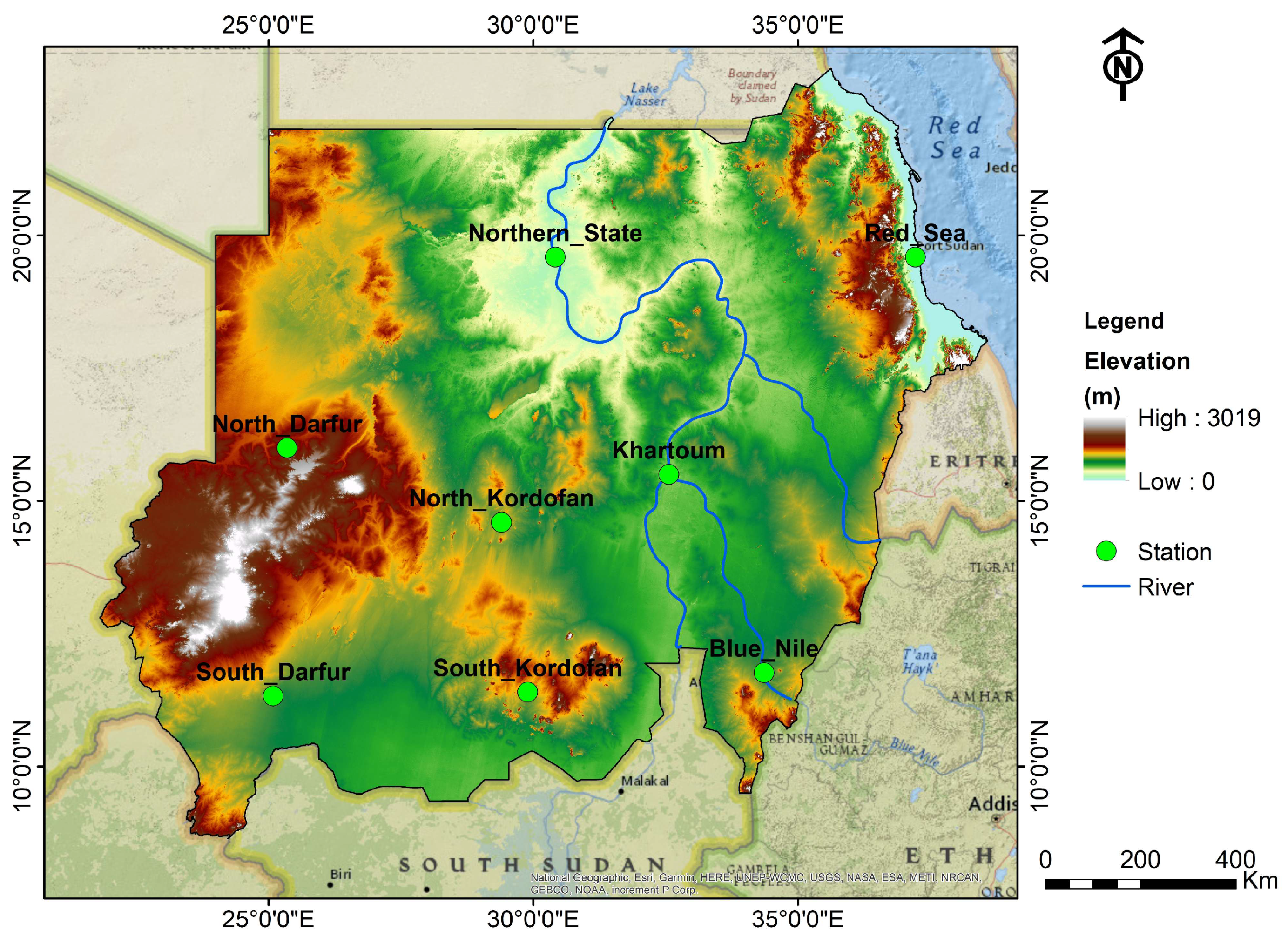
Figure 1. Geographical location of Sudan and its main physiographic features.
Remotesensing 17 03172 g001
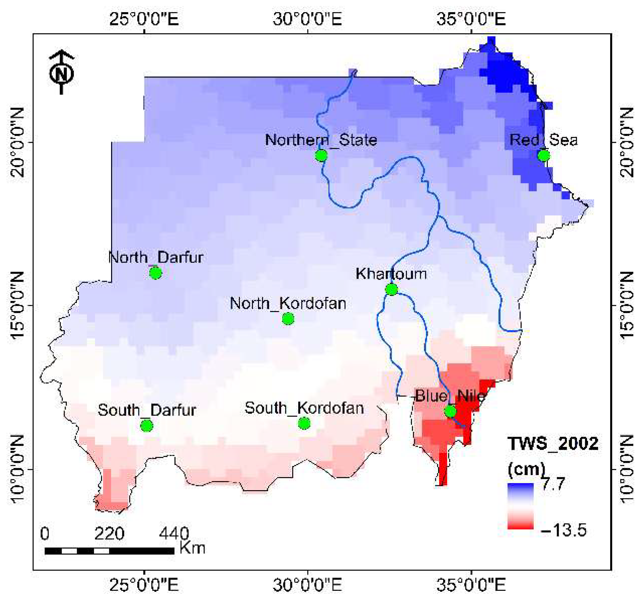
Figure 3. Extent of terrestrial water storage change obtained from GRACE/GRACE-FO CSR of Sudan in 2002.
Remotesensing 17 03172 g003
Figure 4. Performance of the RF model in filling the missing TWS in different stations (KH: Khartoum, RS: Red Sea, SD: South Darfur, ND: North Darfur, SK: South Kordofan, NK: North Kordofan, NS: Northern State, and BN: Blue Nile).
Remotesensing 17 03172 g004
Figure 5. Example of the gab-filling of the TWS in (a) Blue Nile and (b) Khartoum states.
Remotesensing 17 03172 g005
Figure 6. The temporal change in soil moisture in the main states between 2002 and 2025.
Remotesensing 17 03172 g006
Figure 7. Comparison between the groundwater storage change and terrestrial water storage in different zones in Sudan.
Remotesensing 17 03172 g007
Figure 8. Heat maps of monthly Sen’s slope analysis for (a) TWS and (b) GWS showing seasonal variability in trends across eight regional stations.
Remotesensing 17 03172 g008
Figure 9. Example of the groundwater storage change decomposition using STL method.
Remotesensing 17 03172 g009
Figure 10. Representation of the training and validation of the bootsrtapped Bi-LSTM.
Remotesensing 17 03172 g010
Figure 11. Performance of the boostsrapped Bi-LSTM model in predicting GWS in different stations (KH: Khartoum, RS: Red Sea, SD: South Darfur, ND: North Darfur, SK: South Kordofan, NK: North Kordofan, NS: Northern State, and BN: Blue Nile).
Remotesensing 17 03172 g011
Figure 12. Example of the correlation between actual and Bi-LSTM–predicted groundwater storage (GWS) anomalies. The scatter plot illustrates the model’s ability to capture the variability and trend of observed GWS, with points closely aligned along the 1:1 line indicating strong agreement between predicted and observed GWS values.
Remotesensing 17 03172 g012
Figure 13. Example of the prediction, forecasting, and uncetratinity quantification using bootstrapped BiLSTM model in (a) South Kordofan and (b) Blue Nile, and (c) South Darfur.
Remotesensing 17 03172 g013
Figure 14. The estimated Sen slope trend across different stations in Sudan.
Remotesensing 17 03172 g014
Figure 15. Spatial distribution of magnitude of the forecasted GWS trend.
Remotesensing 17 03172 g015
Table 1. The Sen’s slope showing the trend of terrestrial and groundwater storage across the stations.
StationTWS SlopeGWS SlopeGWS_P-Value
Blue Nile0.06800.068361.4 × 10−14
Khartoum0.017252950.017193498.85 × 10−25
Red Sea0.016222080.015595140.002
S_Darfur0.034980880.035847796.4 × 10−10
N_Darfur0.02617250.025911747.70 × 10−45
S_Kordofan0.034605690.034921995.7 × 10−15
N_Kordofan0.025968330.02592672.00 × 10−33
Northern0.01916070.019020349.60 × 10−17
Disclaimer/Publisher’s Note: The statements, opinions and data contained in all publications are solely those of the individual author(s) and contributor(s) and not of MDPI and/or the editor(s). MDPI and/or the editor(s) disclaim responsibility for any injury to people or property resulting from any ideas, methods, instructions or products referred to in the content.