CSTC: Visual Transformer Network with Multimodal Dual Fusion for Hyperspectral and LiDAR Image Classification

Abstract

Convolutional neural networks have made significant progress in multimodal remote sensing image classification, but traditional convolutional neural networks are limited by fixed-size convolutional kernels, which are unable to effectively model and adequately extract contextual information; hyperspectral imagery and LiDAR data have comparatively large information differences, which do not allow for effective information interaction and fusion. Based on this, this paper proposes a multimodal dual fusion network (CSTC) based on the Vision Transformer for the collaborative classification of HSI and LiDAR data. The model is designed through a two-branch architecture: the HSI branch extracts spectral–spatial features by dimensionality reduction using principal component analysis and inputs them into the cross-connectivity feature fusion module; the LiDAR branch mines spatial elevation features through the stacked MobileNetV2 module. The features of the two branches are encoded by a Transformer, and the modal interaction fusion is realized by the cross-attention module for the first time. Then, the features are spliced and input into the secondary Transformer for deep cross-modal fusion, and finally, the classification is completed by the multilayer perceptron. Experiments show that the CSTC model achieves overall classification accuracies of 92.32%, 99.81%, 97.90%, and 99.37% on the publicly available MUUFL dataset, Trento dataset, Augsburg dataset, and Houston2013 dataset, respectively, which is superior to the latest HSI–LiDAR separate classification algorithms. The ablation experiments and model performance evaluation experiments further show that the proposed CSTC model achieves excellent results in terms of robustness, adaptability, and parameter scale.

1. Introduction

Remote sensing is a technology [1] for detecting and identifying the resources and environment on the Earth’s surface in a contactless manner through sensors [2,3] carried by artificial satellites or vehicles. It utilizes electromagnetic wave transmission and reception. Since the 1960s, remote sensing technology has developed rapidly, and it is now widely used in the fields of mineral resource detection [4], environmental monitoring [5], military mapping [6], and urban construction [7]. According to the different types of sensors, remote sensing data can be classified into various types, such as synthetic aperture radar [8], laser radar (LiDAR) [9], infrared light [10], multispectral and hyperspectral [11], and other multi-source remote sensing data [12]. Among them, hyperspectral imagery (HSI) contains not only rich spatial information of features but also detailed spectral information, usually with tens to hundreds of bands, and thus is widely used in land refinement classification [13]. However, hyperspectral image classification faces the challenges of homospectral heterogeneity and homospectral heterogeneity [14]. In contrast, LiDAR data can accurately obtain the 3D structure and elevation information of features, although it usually provides only one or a few bands. Since the spectral information of HSI and the spatial structure, especially the elevation information, of LiDAR form an effective complement, the study of cooperative classification methods based on multi-source data from HSI and LiDAR can effectively solve the problem of “same spectrum, different objects” and thus obtain more accurate classification results.

The traditional land-cover classification based on HSI and LiDAR data can be categorized as a decision fusion-based approach according to the level of information fusion [15]. The core of this type of approach lies in extracting features separately, generating preliminary classification results, and finally integrating them at the decision-making level. The typical process involves the following: spectral or spatial–spectral feature extraction for HSI data; extraction of unique elevation information, echo intensity, and related derived spatial texture features from LiDAR data; application of classifiers such as support vector machines [16], random forests [17], and maximum likelihood methods [18] to classify HSI and LiDAR features independently; and ultimately fusion of the two independent classification results through predefined rules to obtain the optimized final classification map. Representative studies include Dalponte et al. [19], which cross-validated the efficacy of SVM and Gaussian maximum likelihood estimation combined with leave-one-out covariance analysis (GML-LOOC) in fusing HSI and LiDAR data to resolve a complex forest scene; they explored in depth the critical role of different LiDAR echo characteristics and their derived channel data in improving the classification accuracy of HSI, especially in recognizing spectrally similar landform classes; HSI and LiDAR features were classified independently, and the final classification map was obtained by fusing the two independent classification results with a preset rule. Huang et al. [20] evaluated a variety of fusion techniques and proposed an RF-based integration framework, which innovatively integrates HSI spectra, LiDAR elevation, and its derived texture features and employs the built-in feature importance mechanism of the RF model to quantitatively filter the most discriminative feature combinations to output optimized results. Ge et al. [21] developed a fusion framework that extracts extinction profile features from LiDAR point clouds and combines them with local binary pattern (LBP) texture features. This framework adopts Tikhonov-regularized kernel collaborative representation classifiers to process features from different data sources for collaborative decision-making.

In recent years, deep learning-driven data mining [22] and feature fusion techniques have been widely used in the field of multi-source remote sensing data classification [23]. A variety of innovative approaches have emerged from related research: Li et al. [24] proposed a dual-channel A3CLNN framework to realize feature extraction and classification by designing spatial, spectral, and multi-scale attention mechanisms; Zhang, M. et al. [25] used an unsupervised bi-directional autoencoder to reconstruct HSI and LiDAR data and constructed an interleaved perceptual convolutional neural network fusion framework to integrate heterogeneous information and improve classification performance; and Ding et al. [26] developed a global–local Transformer network by fusing convolutional operators with the Transformer architecture’s advantage of learning long-range dependencies, complemented by multi-scale feature fusion and probabilistic decision fusion strategies. Roy et al. [27] focused on capturing multimodal semantic alignment and designed a bilinear attention module that used a K-means-based data enhancement scheme to employ higher-order feature interactions of multi-source data for classification; Zhang, T. et al. [28] proposed a mutual bootstrap attention module, constructed a three-branch convolutional neural network to learn spectral, spatial, and elevation features, and applied a multilevel feature fusion block to integrate shallow and deep information at each branch; and Wang et al. [29] integrated shallow and deep information through multi-scale pyramid convolution to extract features and design a spatio-temporal spectral cross-modal attention module (S2CA), which ultimately formed a classification framework based on multi-scale pyramid fusion. In addition to the more classical HSI and LiDAR classification methods based on convolutional neural networks and the Transformer architecture mentioned above, many scholars have started to explore graph convolutional neural networks [30], Mamba [31] networks, and so on.

Despite the progress of convolutional neural networks in multi-source remote sensing data classification, the following challenges still exist: traditional CNNs are limited by fixed convolutional kernel size, which makes it difficult to effectively model contextual information [32], and there are significant information differences between HSI and LiDAR data, which restrict cross-modal interaction and fusion [33]. For this reason, this paper proposes CSTC-Net, a dual-fusion network based on the Transformer architecture, to realize the collaborative classification of multi-source remote sensing data. The network is mainly composed of two branches and four modules, and the dual branches adopt different feature extraction modules to fully exploit the modal characteristics of HSI and LiDAR data. The extracted features capture the long-range context dependence through the independent Transformer branch, and the output of the dual branches undergoes the first cross-attention interaction. The interacting features are spliced and input into the Transformer for deep feature fusion, and finally, the fused features are classified by a two-layer MLP.

The main contributions of CSTC-Net proposed in this paper are as follows:

• A dual-fusion network structure is constructed, and a symmetric cross-attention module is introduced for the first time after two-branch Transformer encoding to realize the deep interactive fusion of HSI and LiDAR features, which further enhances the cross-modal semantic integration capability through the spliced secondary Transformer fusion and significantly improves the feature characterization capability.
• Different from the traditional parallel network structure, the model fully considers the characteristics of the two types of modal data, purposefully introduces the CCFF module for the spatial–spectral fusion of hyperspectral images in the preprocessing stage, and uses stacked MobileNetV2 blocks to extract the spatial structure features of the LiDAR data, which effectively enhances the discriminative properties of the intra-modal features.
• Experimental results and ablation analyses with multiple state-of-the-art comparative methods on four publicly available datasets show that the model proposed in this paper performs better in the task of multi-source remote sensing image classification, not only outperforming the existing methods in terms of classification accuracy but also achieving a good balance between training and testing efficiency while maintaining a reasonable parameter scale, demonstrating strong practicality and application potential.

2. Related Work

In recent years, with the continuous progress of deep learning technology, the classification accuracy of HSI and LiDAR has continued to improve. In particular, classification methods using Transformer networks have achieved remarkable success. A convolutional neural network (CNN) was combined with a Transformer to achieve collaborative modeling of local spatial details and global spectral features.

Yang et al. [34] designed stackable modal fusion blocks and constructed the Modal-Fusion Visual Transformer (MFViT) framework. Wang, A. et al. [35] proposed a multi-scale attentional feature-fusion network, which combines a hierarchical CNN and Swin Transformer modules to extract multi-scale features and minimize information loss; at the same time, it mines the deep non-spectral features of HSI and LiDAR height information, preserving spatial features and realizing nonlocal sensory-field fusion. Song et al. [36] developed a height information-guided hierarchical fusion separation network (HFSNet), which employs a hierarchical mutual-aid learning mechanism and employs a Transformer and a CNN to encode the spectral information of the HSI and the spatial information of the LiDAR, respectively, in the DSFE module. Wang, M. et al. [37] designed a learnable Transformer with an adaptive gating mechanism (AGMLT) to extract local information through a spectral–spatial adaptive gating mechanism (SSAGM) and used pointwise depth of attention (PDWA) and asymmetric depth of attention (ADWA), respectively, to extract the spectral and spatial information of HSI and LiDAR-DSMM elevation information. Zhao et al. [38] proposed the Bilateral Interactive Hierarchical Adaptive Fusion Network (BIHAF-Net), in which each branch employs a CNN and a Spectral–Spatial Transformer to extract high-level semantic features, enhancing the feature representation capability through a bilateral interactive feedback module and dynamically fusing the features using a cross-modal hierarchical adaptive fusion module, which highlights the importance and preserves details. He et al. [39] combined a Transformer and a CNN, designed a Global–Local Cross-Attention Module (GLCAM) to study deep multimodal features, and constructed a Multi-Level Attention Dynamic Scaling Network (MADNet). Wang, H. et al. [40] proposed a network based on Variable-Scale and Transformer Fusion (MVSTF-Net), which employs similarity calculation to select appropriate scale features and effectively fuses the feature information of HSI and LiDAR through a Cross Self-Attention Fusion (CAF) module. Dai et al. [41] proposed a Cross-Modal Cascade Encoder–Decoder Network (CCEnd-Net), which employs a fuzzy feature extraction module to enhance the anti-aliasing ability of multi-source data and integrates multi-scale data through a cascade encoder–decoder fusion module that combines multi-scale channel-space interaction attention (MCIA) with Transformer-based cross-modal fusion (TCMF).

Despite the progress of existing approaches, such as parallel two-branch CNN–Transformer fusion and single-stage cross-modal attention in multimodal classification, there are still limitations in their architectural design. The parallel two-branch structure extracts intramodal features but lacks a fine-grained interaction mechanism, which leads to the underutilization of complementary cross-modal information. The single-stage fusion framework inputs features directly into the Transformer by splicing, which makes it difficult to model cross-modal complementary information and their inter-modal asymmetric dependencies. Therefore, the CSTC network proposed in this paper aims to solve the above problems through a dual-fusion mechanism: the first cross-attention realizes inter-modal dynamic alignment, and the second Transformer deepens cross-modal semantic integration. This design is superior to single fusion because it can decouple intramodal feature enhancement and inter-modal interaction in a hierarchical manner, avoiding the information confusion caused by direct fusion of heterogeneous features.

3. Research Methodology

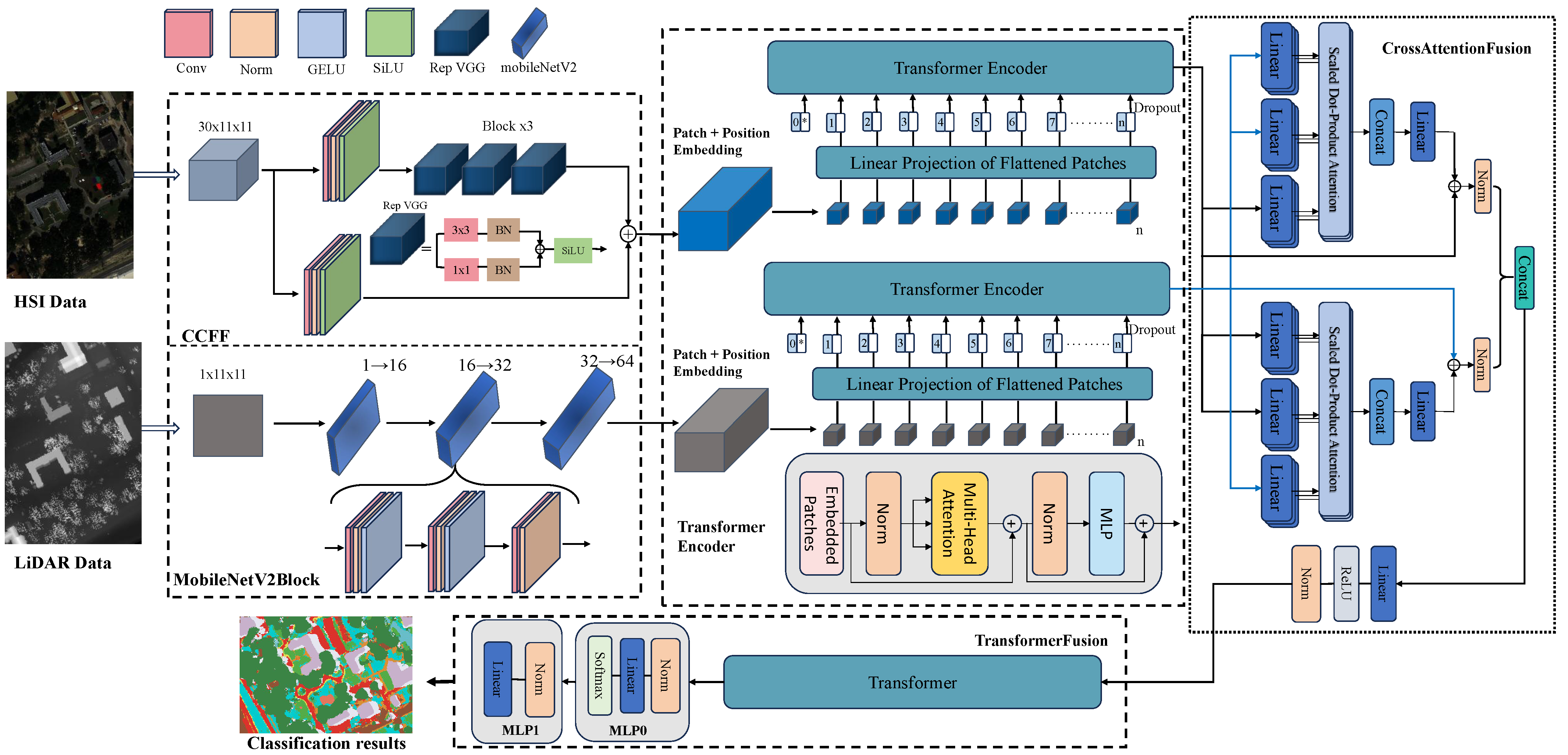
The network framework proposed in this paper for HSI and LiDAR multi-source data classification is shown in Figure 1. The whole process contains two main branches and four core processing stages. Specifically, the HSI data are input into the CCFF module after dimensionality reduction to 30 bands by principal component analysis [42], and the LiDAR single-band data are subjected to in-depth feature extraction using the stacked MobileNetV2 modules. After the two branches undergo in-depth feature mining by an independent Transformer network, inter-modal interactions are realized by the cross-attention fusion module through feature alignment and information complementation. The fused features are augmented with cross-modal features via the Transformer network, and finally, spatial attention weighting and final classification decisions are achieved using dual-MLP classification heads. The architecture fully exploits the complementary information of multi-source data through the four-stage processing of cascaded feature extraction, parallel Transformer mining, cross-attention fusion, and secondary feature enhancement. The specific algorithms of the proposed model are shown below.

3.1. Bimodal Feature Extraction Flow

In order to fully exploit the complementary spatial–spectral information of HSI and LiDAR images, this paper uses a bimodal feature extraction flow, which is a module that performs in-depth feature mining on HSI and LiDAR data and provides more discriminative modal characterization for subsequent feature enhancement and feature fusion.

3.1.1. Hyperspectral Branch

Since hyperspectral images are characterized by high dimensionality and information redundancy, this paper first uses principal component analysis to downscale the hyperspectral images, retaining only 30 main components and thus significantly reducing the complexity of the computation. The downsized data are expressed as $X_{HSI}\in {\mathbb{R}}^{B\times 30\times h\times w}$, where B denotes the batch size and $h\times w$ denotes the spatial dimensionality of the image. The downscaled HSI data are fed into the Cross-Connected Feature-Fusion (CCFF) module for feature extraction. This module consists of two parallel convolutional paths with a residual feature enhancement module, which is processed as follows.

$$X_1=SiLU\left(Norm\left({Conv}_{1\times 1}^{\left(2\right)}\left(X_1\right)\right)\right)$$

(1)

$$X_1^{\prime }=RepVGG\left(X_1\right)=SiLU\left(Norm\left({Conv}_{1\times 1}^{\left(2\right)}\left(X_1\right)\right)+BN\left({Conv}_{3\times 3}^{\left(3\right)}\left(X_1\right)\right)\right)$$

(2)

$$X_1^{‴}={RepVGG}^3\left(X_1\right))$$

(3)

where $RepVGG$ of two parallel convolutional paths denotes a module consisting of multiple residual block stacks, ${Conv}_{1\times 1}^{\left(2\right)}$ and ${Conv}_{3\times 3}^{\left(3\right)}$ denote the included parallel $1\times 1$ vs. $3\times 3$ convolutional paths, and $SiLU$ denotes the activation function. The final output of the HSI feature is:

$$F_1=X_1^{‴}+X_1$$

(4)

The hyperspectral branch output, $F_1\in {\mathbb{R}}^{B\times 64\times h\times w}$, effectively enhances the spatial structure modeling capability by using parallel convolutional paths and residual connections to capture multi-scale information.

3.1.2. LiDAR Branch

The LiDAR data comprise a single-channel elevation map. In order to fully explore its spatial hierarchical features, this paper adopts MobileNetV2 for feature extraction, as it has a strong feature extraction capability and maintains low model complexity. The original input LiDAR image is denoted as $X_{LiDAR}\in {\mathbb{R}}^{B\times 1\times h\times w}$, where B denotes the batch size and $h\times w$ denotes the spatial dimension of the image. The specific roles of the individual modules are as follows.

The original single-channel LiDAR elevation maps are first extended in dimension by $1\times 1$ convolution, and then finer-grained local spatial variations are learned by $3\times 3$ convolution to enhance sensitivity to object shape and texture variations in LiDAR images. Finally, the abstract high-level features and globally integrated features are further extracted by $1\times 1$ convolution.

$$Y_1=GELU\left(BN\left(Con{v}_{1\times 1}\left(X_{LiDAR}\right)\right)\right)$$

(5)

$$Y_2=GELU\left(BN\left(DWCon{v}_{3\times 3}\left(Y_1\right)\right)\right)$$

(6)

$$Y_3=BN\left(Con{v}_{1\times 1}\left(Y_2\right)\right))$$

(7)

GELU is the activation function, and the channel change is achieved after passing through three MobileNetV2 modules, as follows: 1→ 16→32→64. Although the inverted residual structure is not integrated, the linear bottleneck design adopted in this module effectively optimizes the model’s image classification and characterization ability and simultaneously improves the robustness of multimodal remote sensing image fusion. The final LiDAR branch output $F_2\in {\mathbb{R}}^{B\times 64\times h\times w}$ is obtained.

3.2. Transformer Feature Enhancement

Before using the Transformer network to model its spatial relationships, the data need to be converted to a sequence representation, and positional encoding must be introduced in order to extract global contextual semantic information with this structure. Take the HSI branch as an example: the output feature map of the branch, $F_1\in {\mathbb{R}}^{B\times 64\times h\times w}$, is first converted to a 2D patch sequence by a spatial flattening operation to get $F_1^{\prime }\in {\mathbb{R}}^{B\times N\times 64}$, where $N=h\times w$ represents the total number of spatial locations. Each position is considered a token, and the number of channels $C=64$ is projected to the hidden dimension D of the Transformer through the linear mapping layer to get $z_1\in {\mathbb{R}}^{B\times N\times D}$. Since the Transformer itself does not have the ability to process the position information in the sequence, a learnable position encoding is introduced to get $z_1^{pos}$ in order to guide the model to learn the spatial order. Finally, $z_1^{Drop}$ is obtained through a dropout operation to maintain the model’s generalization ability, and the obtained feature sequence is input into the Transformer encoder module for feature enhancement. The overall transformation process is as follows:

$$z_1^{Drop}=Dropout\left(F_1^{\prime }{W}_e+b_e+P[:,:N,:]\right)$$

(8)

where $W_e\in {\mathbb{R}}^{C\times D}$ is the linear mapping weight, $b_e$ is the bias term, and $P[:,:N,:]$ is the learnable positional encoding. The input feature sequences are fed into the multi-head self-attention module ($MSA$) to capture the rich contextual dependencies from different subspaces. The output of this module is the result of splicing multiple attention heads:

$$MSA\left(x\right)=Concat\left(hea{d}_1,hea{d}_2\dots hea{d}_n\right)$$

(9)

Each attention head is computed using the following equation, which calculates the similarity between different tokens by scaling the dot product attention mechanism:

$${head}_i=softmax\left({\displaystyle \frac{Q_i{K}_i^T}{\sqrt{d}}}\right)V_i$$

(10)

In this case, the query, key, and value are obtained from the input features X by linear transformation: $Q=X{W}_Q, K=X{W}_K, V=X{W}_V$, $W_Q, W_K, W_V\in {\mathbb{R}}^{D\times d}$, and in order to improve the representation ability of the model, a feed-forward neural network ($FFN$) is also applied after each attention module:

$$FFN\left(x\right)=W_2·GELU\left(W_{1}X+b_1\right)+b_2$$

(11)

The entire Transformer encoder layer is stabilized for training and gradient propagation using residual concatenation and LayerNorm. The specific forward-propagation process for each layer is as follows:

$$x^{\prime }=X+MSA\left(layerNorm\left(X\right)\right)$$

(12)

$$x^{″}=x^{\prime }+FFN\left(layerNorm\left(X\right)\right)$$

(13)

$X\in {\mathbb{R}}^{B\times N\times D}$ denotes the input sequence of the Transformer, which is passed through l layers to get the Transformer output

$$X_1^{\mathrm{out}}=Transformer\left(z_1^{\mathrm{Drop}}\right)\in R^{B\times N\times D}$$

(14)

This output contains global spatial context information and is used as input for subsequent feature fusion, effectively improving the model’s performance, and the output of the LiDAR branch is the same as above.

3.3. First Cross-Attention Fusion

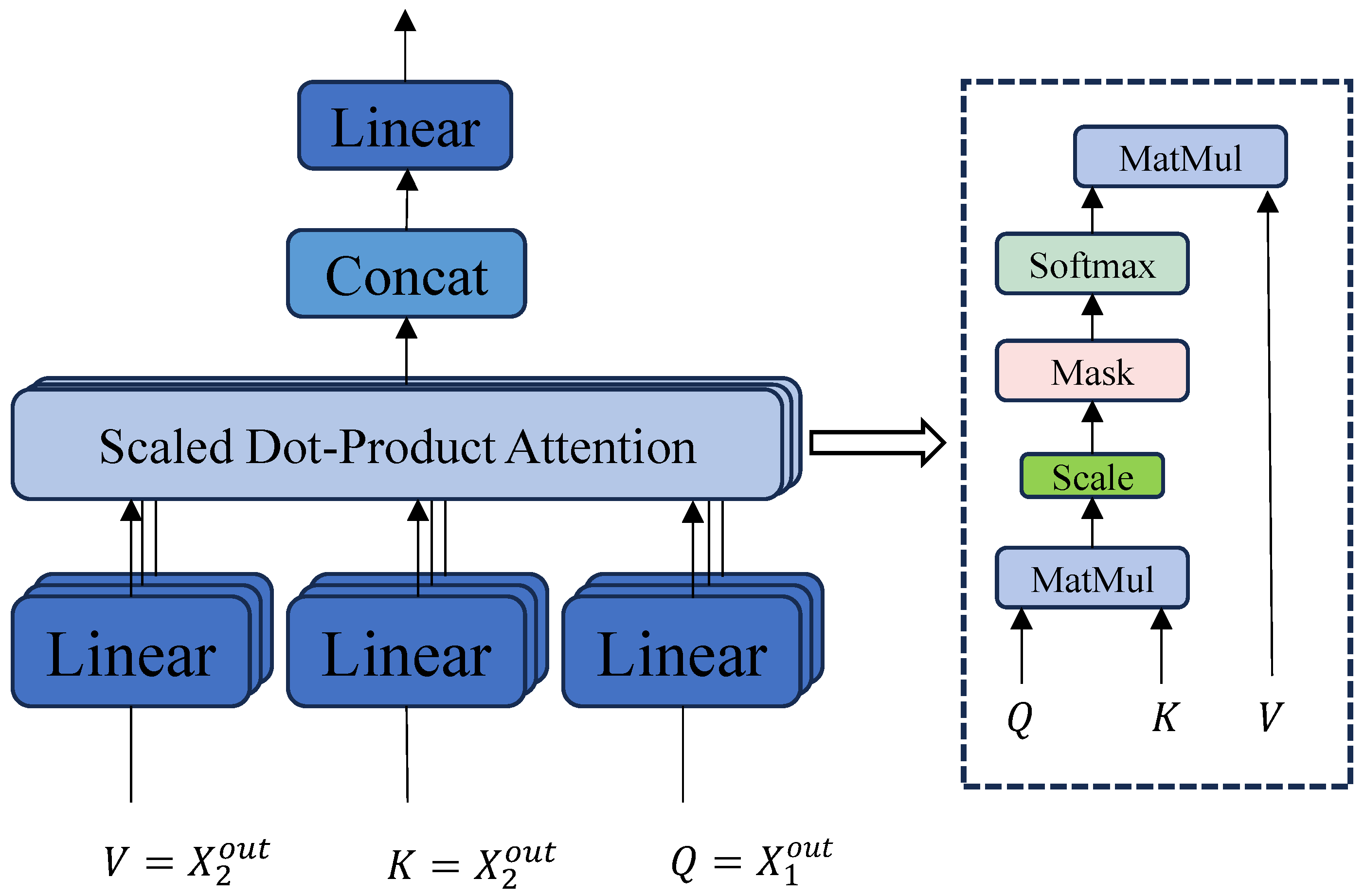
The hyperspectral branch output $X_1^{out}\in {\mathbb{R}}^{B\times N\times D}$ and the LiDAR branch output $X_2^{out}\in {\mathbb{R}}^{B\times N\times D}$ are obtained through a bimodal feature extraction flow and Transformer feature enhancement, and in order to realize the deep inter-modal interactions, the module uses two symmetric multi-head self-attention substructures, as shown in Figure 2:

The HSI is used to sense the LiDAR information, the hyperspectral feature $X_1^{out}$ is used as the query vector (Q), and the LiDAR feature $X_2^{out}$ is used as the key (K) and the value (V), which guides the HSI to focus on the spatial–structural information provided by LiDAR to realize the enhancement of spatial sensitivity:

$$\widetilde{X_1}=MSA\left(Q=X_1^{\mathrm{out}},K=X_2^{\mathrm{out}},V=X_2^{\mathrm{out}}\right)$$

(15)

Using LiDAR to perceive HSI spectral features, the spectral discriminative feature information is extracted from HSI using the LiDAR feature $X_2^{out}$ as Q and the LiDAR feature $X_1^{out}$ as K and V so as to enhance its semantic expression capability. The following is obtained:

$$\widetilde{X_2}=MSA\left(Q=X_2^{\mathrm{out}},K=X_1^{\mathrm{out}},V=X_1^{\mathrm{out}}\right)$$

(16)

where each attention head is computed in the same form as Equation (10). In order to preserve the original modal information while cross-modeling and to enhance the training stability, residual connectivity with LayerNorm is introduced:

$$\widetilde{Z_1}=\mathrm{LayerNorm}\left(X_1^{\mathrm{out}}+\widetilde{X_1}\right)$$

(17)

$$\widetilde{Z_2}=\mathrm{LayerNorm}\left(X_2^{\mathrm{out}}+\widetilde{X_2}\right)$$

(18)

The two processed sequence features $\widetilde{Z_1}$ and $\widetilde{Z_2}$ are spliced in the channel dimension, and the fused features are compressed in dimension by linear transformation with a nonlinear activation function and a normalization layer to achieve a compact representation of the modal joint features. Finally, the output of the fused features is obtained:

$$Z=Norm\left(ReLU\left(Linear\left(Concat\left(\widetilde{Z_1},\widetilde{Z_2}\right)\right)\right)\right)$$

(19)

where the output shape Z is recovered as $Z\in {\mathbb{R}}^{B\times N\times C}$, where B is the batch size, N is the number of features, and C is the feature dimension.

3.4. Transformer Secondary Feature Fusion and MLP Classification

After the fusion of the completed feature sequences $Z\in {\mathbb{R}}^{B\times N\times C}$, the module further extracts the global contextual relationships through the Transformer encoder and then utilizes an attention-weighted feature aggregation mechanism to generate the final image-level feature vectors that are used for classification prediction.

The Transformer module consists of several layers of multi-head self-attention and feed-forward networks, with residual connections and layer normalization mechanisms to enhance training stability. This Transformer architecture is consistent with the formulas and networks used in vignette 3.2, which ultimately results in a quadratic fusion feature output:

$$Z^{\prime }=Transformer\left(Z\right)\in R^{B\times N\times C}$$

(20)

Subsequently, in order to aggregate the information of the whole sequence, a simplified attention mechanism is used as an aggregated weight generator:

$$\alpha =softmax\left(Linear\left(LayerNorm\left(Z^{\prime }\right)\right)\right)$$

(21)

where $\alpha \in {\mathbb{R}}^{B\times N\times 1}$. This step is implemented through the $MLP1$ module to generate an attention score for each sequence. All sequences are aggregated into a single global feature representation by means of attentional weighting: ${\alpha }^T{Z}^{\prime }\in {\mathbb{R}}^{B\times D}$. Finally, the aggregated global feature y is input into $MLP2$ for classification prediction.

$$\widehat{y}=Linear\left(LayerNorm\left({\alpha }^T{Z}^{\prime }\right)\right)$$

(22)

where $y\in {\mathbb{R}}^{B\times C}$, B is the batch size, C is the number of categories, and the output is the category probability for each sample. The whole algorithm runs as shown in Algorithm 1.

Algorithm 1: The proposed CSTC algorithm.
	Input: Hyperspectral images (HIS), LiDAR images, training labels, Epoch: 200
	Output: Predicted category label for each pixel point
	Initialization: Set the random seed and initialize all module parameters of the CSTC network.
	1. Perform PCA dimensionality reduction on HSI to 30 dimensions while keeping LiDAR in its original single-channel form.
	2. HSI input CCFF module extracts spectral–spatial features; Formulas (1)–(4).
	3. Spatial features are extracted from LiDAR images using three layers of MobileNetV2 blocks; Formulas (5)–(7).
	4. The two-modal features are separately input into the Transformer encoder to enhance contextual information; Formulas (8)–(14).
	5. Achieve modal interaction fusion through dual cross-attention modules; Formulas (15)–(19).
	6. Re-input the merged features into the Transformer for deep semantic fusion, referring to 4.
	7. Attention-weighted feature aggregation, MLP classifier output category probability; Formulas (20)–(22).
	8. Backpropagation optimization parameters.
	9. Repeat steps 1–8 until training is complete.
	Use the trained model to make predictions on the test data and output a classification map.

4. Experimental Data and Environment

This paper selects four representative public multimodal remote sensing datasets as the basis for the experiment. These datasets cover different regions and types of land features and are highly diverse and challenging.

4.1. Experimental Data

This subsection presents basic information on four multimodal remote sensing classification datasets commonly used for hyperspectral and LiDAR, including the MUUFL, Trento, Augsburg, and Houston2013 datasets.

MUUFL dataset: Collected from the University of Southern Mississippi, Gulf Park Campus, USA. The spatial scale of the image is 325 × 220 pixels with a spatial resolution of 1 m. The hyperspectral data contain 72 bands, and the LiDAR data are captured by the ALTM sensor (Made by Teledyne Optech, Concord, Ontario, Canada), which contains two rasters with a wavelength of 1.06 μm. It covers 11 types of features, such as Trees, Grass Pure, and Road Materials, with a total of 53,687 samples.

Trento dataset: Acquired from the suburban area of Trento, Italy, with an image size of 600 × 166 pixels and a resolution of 1 m. The hyperspectral data contain 63 bands (0.42–0.99 μm); LiDAR is single-band data. A total of 30,214 labeled samples were classified into six feature classes, of which 819 were used for training and 29,395 for testing.

Augsburg dataset: Covers the Augsburg region in Germany. HSI data were acquired by the HySpex hyperspectral sensor (Made by Norsk Elektro Optikk AS, Oslo, Norway) (180 bands, 0.4–2.5 μm), LiDAR-based DSM data were acquired by DLR-3K system (Made by the German Aerospace Center, Cologne, Germany). The DSM data have only one raster, with an image size of 332 × 485 pixels and a resolution of 30 m, and contain 7 types of features, such as Forest, Residential Area, and Low Plants, with a total of 78,294 samples.

Houston2013 (Houston) dataset: Published by the U.S. Airborne Laser Mapping Center in conjunction with the HSI Analysis Group. The spatial scale of the image is 340 × 1905 pixels, the resolution is 2.5 m, and the hyperspectral data contain 144 bands (0.38–1.05 μm). The LiDAR data are single-band. There are 15 classes of features, with a total of 15,029 samples, 1125 in the training set and 13,904 in the test set. The sample distribution is shown in

Table 1. Table of sample sizes for training and testing.

Data Name	ID	Category	Train	Test	ID	Category	Train	Test
Muufl	1	Trees	150	23,096	7	Building Shadow	150	2083
	2	Grass Pure	150	4120	8	Building	150	6090
	3	Grass Groundsurface	150	6732	9	Sidewalk	150	1235
	4	Dirt and Sand	150	1676	10	Yellow Curb	150	33
	5	Road Materials	150	6537	11	Cloth Panels	150	119
	6	Water	150	316
Trento	1	Apples	129	3905	4	Woods	154	8969
	2	Buildings	125	2778	5	Vineyard	184	10,317
	3	Ground	105	374	6	Roads	122	3052
Augsburg	1	Forest	675	12,832	5	Allotment	28	547
	2	Residential Area	1516	28,813	6	Commercial Area	82	1563
	3	Industrial Area	192	3659	7	Water	76	1454
	4	Low Plants	1342	25,515
Houston	1	Healthy Grass	75	1176	9	Road	75	1177
	2	Stressed Grass	75	1179	10	Highway	75	1152
	3	Synthetic Grass	75	622	11	Railway	75	1160
	4	Trees	75	1169	12	Parking Lot 1	75	1158
	5	Soil	75	1167	13	Parking Lot 2	75	394
	6	Water	75	250	14	Tennis Court	75	353
	7	Residential	75	1193	15	Running Track	75	585
	8	Commercial	75	1169

and Figure 3.

4.2. Experimental Environment

The hardware platform GPU model for running the experiment is Intel(R) Core(TM) i5-12600, the host memory is 32G, the GPU model is NVIDIA GeForce RTX5070, and the model running environments are Python 3.9.21 and PyTorch2.8.0+cu128.

In order to ensure the fairness and impartiality of the experiments, all the comparison algorithms were run in the same computer environment. To ensure the reproducibility of the experiments, we set the random seed to 0. Each experiment was repeated once individually, the training cycle was 200 rounds, the learning rate was fixed to 0.0005, the number of bands in the hyperspectral image after downscaling by PCA was 30, and the batch size was fixed at 144. To evaluate the performance of CSTC in hyperspectral remote sensing image classification, this paper uses the state-of-the-art hyperspectral and LiDAR data classification networks from 2022 to 2024 for comparison. The comparison algorithms used are CrossHL [43], ExViT [44], HCT [45], MS2CANet [29], and S2ATNet [46]. The CrossHL algorithm proposes a cross-modal Transformer network that fuses hyperspectral and LiDAR data and realizes efficient fusion and joint classification of multi-source remote sensing information by introducing a cross-modal high- and low-dimensional attention mechanism and a heterogeneous convolution module. The ExViT algorithm aims to improve the classification performance based on the Transformer framework through modal feature extraction, projection alignment, and cross-modal attention fusion. The HCT algorithm performs multimodal information fusion through hierarchical convolutional feature extraction, tokenization, and a cross-modal Transformer encoder to improve the accuracy of land cover and utilization classification. The MS2CANet algorithm proposes a multi-scale spatio-spectral cross-modal attention network that integrates multi-scale convolutions, channel-space attention mechanisms (EFR), and cross-attention mechanisms (SA & SE) to enhance multi-modal feature representation capabilities. The S2ATNet algorithm designs a selective spectral–spatial aggregation Transformer network, utilizing a dual-branch Transformer architecture and DualBlock modules to finely model intra-modal and inter-modal feature dependencies, thereby improving classification performance.

In order to comprehensively evaluate the performance of the proposed CSTC algorithm, four quantitative metrics are used in this paper: overall accuracy (OA), average accuracy (AA), the Kappa coefficient, and the classification accuracy for each category. At the same time, this is complemented with the visualization of the classification results for qualitative analysis. In the discussion section, ablation experiments, model parameter quantities, and training/testing elapsed time statistics are further supplemented. The experimental results verify the robustness and excellent classification performance of the CSTC algorithm.

5. Experimental Results

In this section, comparative experimental analyses and ablation analyses are conducted for the key modules of the proposed multimodal fusion model, and the proposed CSTC model achieves excellent results in terms of robustness, adaptability, and ablation experiments.

5.1. Comparison Results of Different Algorithms on Four Datasets

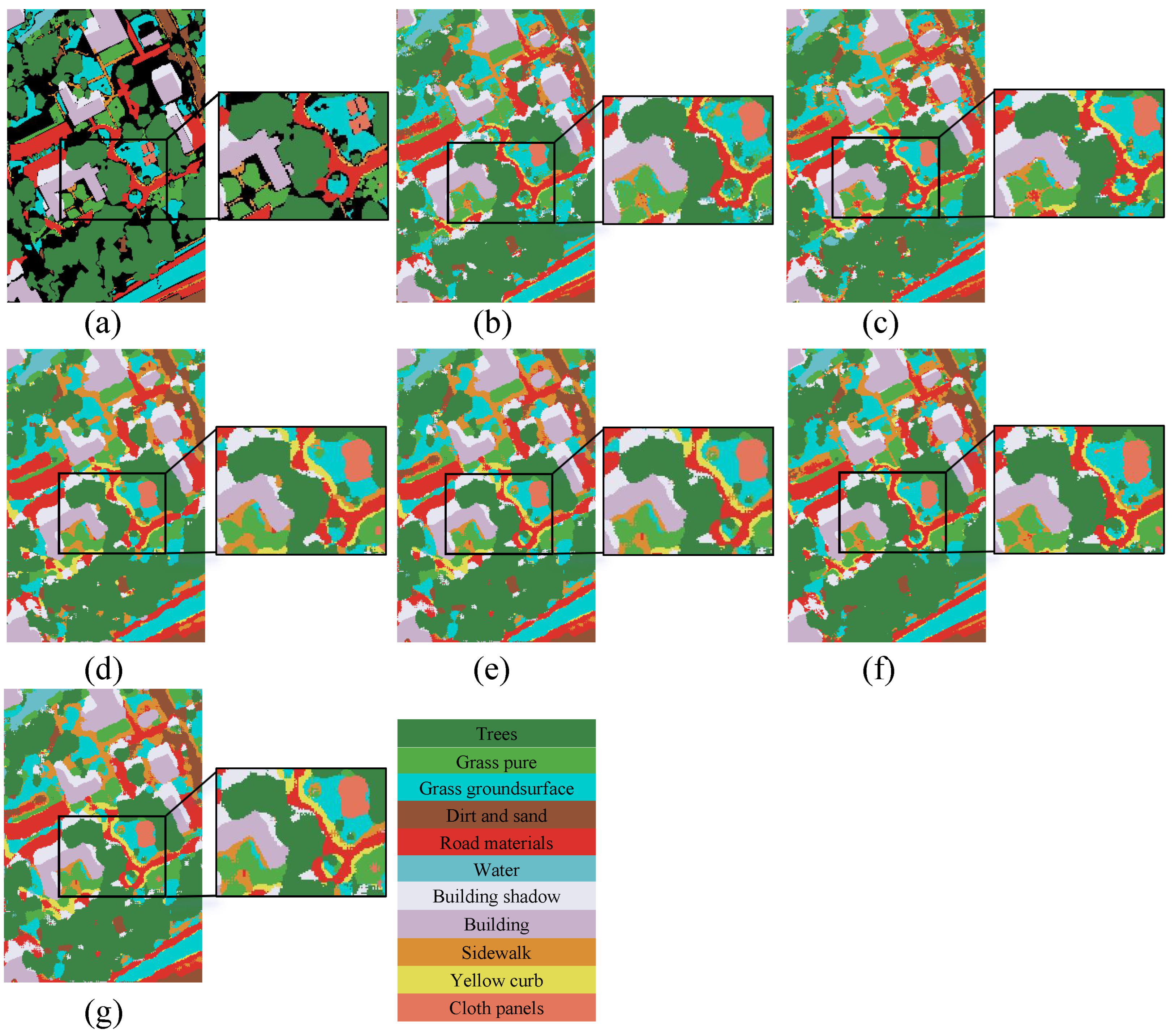
For the MUUFL dataset, as shown in Figure 4 of the classification results and

Table 2. Classification results of different comparison algorithms on the MUUFL dataset.

MUUFL	CrossHL	ExViT	HCT	MS2CANet	S2ATNet	Proposed
1	89.11	90.05	89.32	88.71	89.70	92.19
2	86.77	85.70	85.15	88.01	90.24	91.38
3	77.84	84.12	79.81	78.73	84.06	86.38
4	96.90	95.64	95.11	96.60	98.21	96.84
5	90.39	89.98	88.30	86.58	91.59	95.07
6	100.00	100.00	100.00	100.00	100.00	100.00
7	89.77	91.31	94.24	92.17	92.03	94.48
8	96.39	96.04	94.84	93.73	95.85	96.35
9	71.74	77.81	76.60	70.20	84.62	83.08
10	90.91	100.00	90.91	100.00	100.00	93.94
11	100.00	100.00	99.16	100.00	100.00	100.00
OA (100%)	88.44	89.66	88.45	87.74	90.31	92.32
AA (100%)	89.98	91.88	90.31	90.43	93.30	93.61
Kappa (100%)	84.90	86.49	84.94	84.03	87.33	89.89

of the classification performance, the CSTC proposed in this paper achieves 92.32% OA, 93.61% AA, and 89.89% Kappa, all of which are better than those achieved by the latest comparison algorithm. Compared with the ExViT algorithm, the values of OA, AA, and Kappa are improved by 2.66%, 1.73%, and 3.4%, respectively. The reason is that although the ExViT algorithm implements local spatial modeling, inter-modal interaction, and global modeling modal fusion in the Transformer architecture, it only performs Transformer fusion by splicing and does not use finer-grained cross-attention or other interaction methods. Due to the large number of network parameters, this may lead to overfitting for the labeled samples. The CSTC algorithm introduces a cross-attention interaction method and adopts double-Transformer modal fusion so that Trees, Grass Pure, Road Materials, etc., achieve excellent classification results even when a small number of labeled samples are used for training.

For the Trento dataset, the classification performance of each comparison algorithm is shown in

Table 3. Classification results of different comparison algorithms on the Trento dataset.

Trento	CrossHL	ExViT	HCT	MS2CANet	S2ATNet	Proposed
1	99.33	98.80	99.72	99.67	98.46	99.67
2	99.50	99.42	99.03	97.59	98.31	99.82
3	100.00	100.00	100.00	100.00	100.00	100.00
4	100.00	100.00	100.00	100.00	100.00	100.00
5	99.76	99.97	100.00	99.99	99.93	99.98
6	96.85	98.95	98.17	94.89	98.66	98.82
OA (100%)	99.45	99.67	99.68	99.19	99.47	99.81
AA (100%)	99.24	99.52	99.49	98.69	99.23	99.71
Kappa (100%)	99.27	99.55	99.57	98.92	99.29	99.74

, and the CSTC model proposed in this paper achieves the highest OA, AA, and Kappa metrics. Nevertheless, the remaining methods perform equally well on Trento. From the classification visualization results in Figure 5 and the number of training/testing samples in Table 1, it can be seen that the Trento dataset has small coverage, a clear texture structure, clear boundaries of categories such as Buildings, Forest, and Roads, and significant spectral differences between the categories, which enables each algorithm to fully extract discriminative features and achieve high classification accuracy. The MS2CANet algorithm uses multi-scale PyConv+ECA+spatial attention, but the lack of spatial modeling and the rough fusion method lead to the loss of structural features such as Buildings and Roads, so the classification accuracies on Buildings and Roads are only 97.59% and 94.89%.

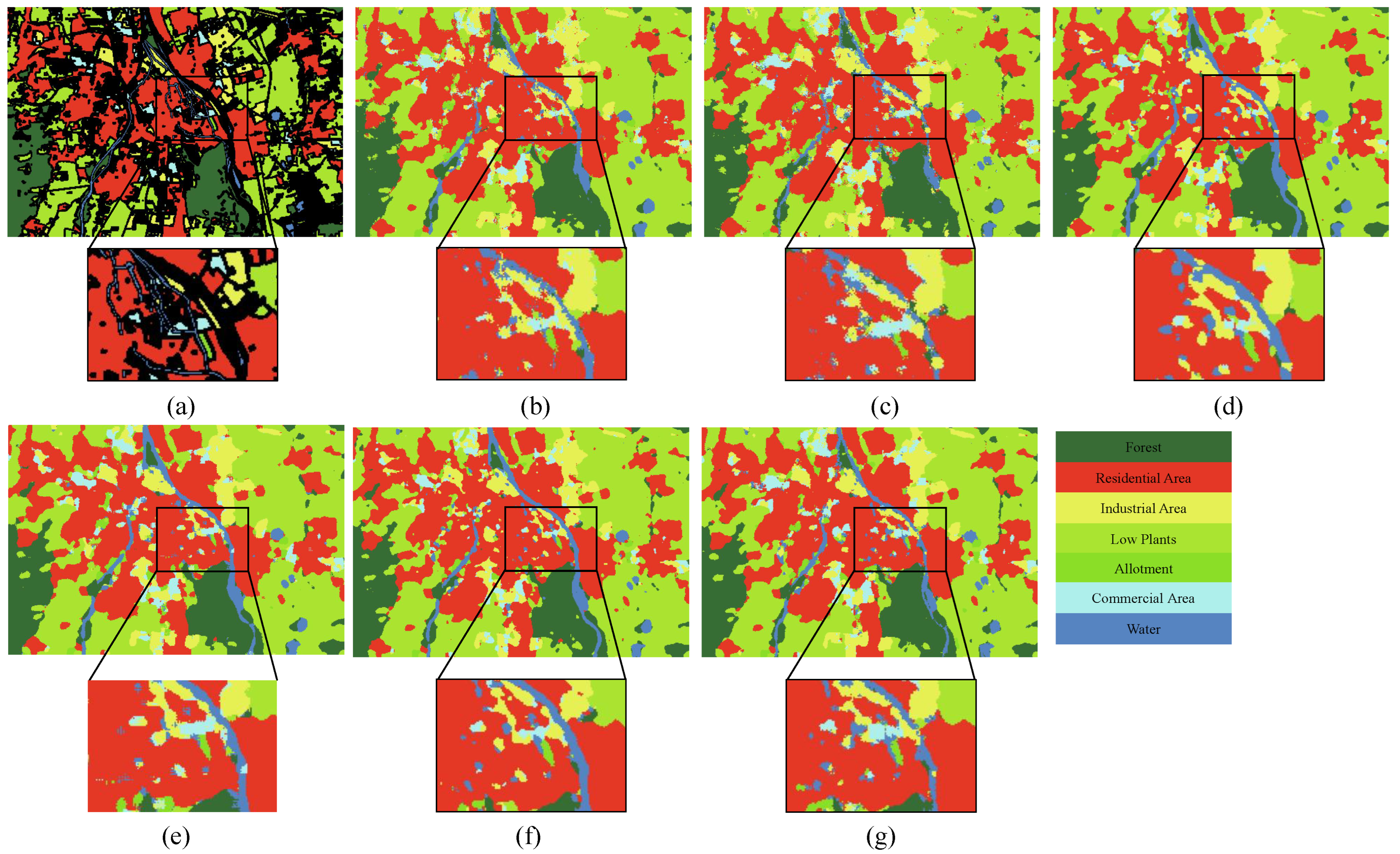
As shown in Figure 6, the CSTC algorithm is more adaptable to the fine-grained, sample-imbalanced classes in the Augsburg data. Although the CrossHL modle is simpler and faster to train, it has shallow cross-modal interaction capability and difficulty modeling complex relationships. HCT is based on the complex Transformer model, leading to complex training, and it is sensitive to sample size.

In Classification

Table 4. Classification results of different comparison algorithms on the Augsburg dataset.

Augsburg	CrossHL	ExViT	HCT	MS2CANet	S2ATNet	Proposed
1	99.24	99.09	98.72	99.16	99.06	99.39
2	98.88	99.03	98.67	98.79	99.01	99.22
3	88.00	88.38	95.55	94.78	91.66	94.75
4	99.38	98.93	99.49	99.39	99.53	99.46
5	81.90	77.33	91.77	78.24	74.77	87.02
6	50.80	62.76	51.18	64.56	59.50	72.17
7	65.96	62.17	70.77	66.09	69.39	70.84
OA (100%)	96.80	96.84	97.21	97.35	97.25	97.90
AA (100%)	83.45	83.96	86.59	85.86	84.70	88.98
Kappa (100%)	95.40	95.46	96.01	96.20	96.05	96.99

, HCT achieves only a small advantage over the CSTC algorithm in the weak categories Industrial Area, Low Plants, and Allotment, and the classification accuracy of the two in Commercial Area is about 20% lower than that of the CSTC algorithm, indicating that the proposed model is more accurate in the Augsburg dataset compared with CrossHL and HCT. The proposed model is a better HSI–LiDAR multimodal classification scheme that can significantly improve weak class performance and overall generalization ability while maintaining the main class accuracy.

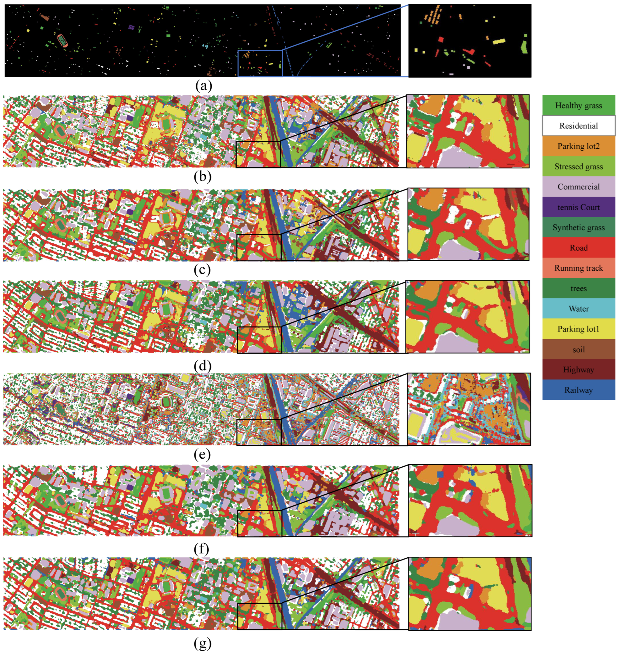
For the Houston dataset, as shown in Figure 7 and

Table 5. Classification results of different comparison algorithms on the Houston dataset.

Houston	CrossHL	ExViT	hct	MS2CANet	S2ATNet	Proposed
1	98.55	97.87	99.74	99.49	99.40	99.06
2	98.90	98.47	99.15	99.32	98.39	98.64
3	100.00	99.68	100.00	99.84	100.00	100.00
4	98.63	98.29	99.83	99.40	98.72	99.23
5	100.00	100.00	100.00	100.00	99.91	100.00
6	98.00	99.60	100.00	100.00	100.00	100.00
7	92.37	98.91	99.08	98.49	95.05	99.50
8	97.09	95.47	97.69	94.10	98.72	99.32
9	96.60	97.28	98.81	98.30	98.73	99.75
10	97.40	97.48	100.00	100.00	100.00	99.13
11	100.00	99.91	100.00	100.00	100.00	100.00
12	99.57	98.45	98.36	98.79	98.36	98.53
13	97.21	97.46	98.48	98.48	97.21	98.22
14	100.00	100.00	100.00	100.00	100.00	100.00
15	100.00	100.00	100.00	100.00	100.00	100.00
OA (100%)	98.12	98.40	99.34	98.93	98.84	99.37
AA (100%)	98.29	98.59	99.41	99.08	98.97	99.43
Kappa (100%)	97.96	98.27	99.28	98.84	98.75	99.32

, there are significant differences in the classification effects of HCT, MS2CANet, S2ATNet, and CSTC. HCT performs well in areas with clear feature boundaries. S2ATNet realizes dynamic weighted fusion of HSI and LiDAR information through the introduction of adaptive spatial-spectral cross-talk and is particularly robust to areas with severe occlusion or unclear texture, thus achieving excellent performance in heterogeneous areas. In contrast, MS2CANet is more robust in complex urban scenes, such as Buildings and Low Vegetation. S2ATNet achieves excellent performance in heterogeneous area classification by introducing an adaptive spatial–spectral cross-attention mechanism, which realizes the dynamic weighted fusion of HSI and LiDAR information, especially in areas with severe occlusion or unclear texture. In contrast, MS2CANet does not differentiate between easily mixed categories, such as Buildings and Low Vegetation, in complex urban scenes. As is obvious in Figure 7, MS2CANet categorizes a large number of Trees and Grass as Water, leading to a large number of white pixels on the classification map. The CSTC method improves the network model’s in-depth understanding of complex spatial texture and spectral features through a strong feature extraction module and multi-stage feature fusion. In the Houston dataset, the accuracy of CSTC reaches 100% for the six easy-to-classify categories, such as Synthetic Grass, Soil, and Water, and for the remaining nine categories, the classification accuracy is 98% or more. On the classification results map, the noise region is significantly reduced, and the segmentation is cleaner and more accurate.

In summary, the comparative analysis of five state-of-the-art comparative algorithms on four classical HSI–LiDAR datasets shows that the CSTC-based HSI–LiDAR remote sensing image classification algorithm proposed in this study achieves excellent classification results in a number of metrics, such as overall classification accuracy, average accuracy, and the Kappa coefficient.

5.2. Ablation Experiments

In order to systematically evaluate the independent contribution and synergistic mechanism of the CCFF, MobileNetV2, and CrossAttentionF modules, this study carries out seven sets of controlled tests on four datasets. As shown in

Table 6. Results of CSTC ablation experiments on the MUUFL dataset.

Cases	Component			Indicators
	CCFF	MobileNetV2	CrossAttentionF	OA (%)	AA (%)	Kappa (%)
1	√	×	×	90.88	92.94	88.04
2	√	√	×	91.74	93.14	89.14
3	×	×	√	92.11	94.32	89.63
4	√	×	√	90.78	93.34	87.96
5	×	√	√	91.27	93.88	88.56
6	×	√	×	90.01	93.38	86.98
7	√	√	√	92.32	93.61	89.89

,

Table 7. Results of CSTC ablation experiments on the Trento dataset.

Trento	Component			Indicators
	CCFF	MobileNetV2	CrossAttentionF	OA (%)	AA (%)	Kappa (%)
1	√	×	×	99.70	99.53	99.60
2	√	√	×	99.77	99.66	99.69
3	×	×	√	99.60	99.37	99.46
4	√	×	√	99.76	99.66	99.68
5	×	√	√	99.79	99.67	99.71
6	×	√	×	99.65	99.42	99.53
7	√	√	√	99.81	99.71	99.74

,

Table 8. Results of CSTC ablation experiments on the Augsburg dataset.

Augsburg	Component			Indicators
	CCFF	MobileNetV2	CrossAttentionF	OA (%)	AA (%)	Kappa (%)
1	√	×	×	97.77	87.61	96.80
2	√	√	×	97.84	89.26	96.90
3	×	×	√	97.32	86.53	96.17
4	√	×	√	97.70	88.41	96.70
5	×	√	√	97.06	85.04	95.79
6	×	√	×	97.33	85.99	96.17
7	√	√	√	97.90	88.98	96.99

and

Table 9. Results of CSTC ablation experiments on the Houston dataset.

Houston	Component			Indicators
	CCFF	MobileNetV2	CrossAttentionF	OA (%)	AA (%)	Kappa (%)
1	√	×	×	99.19	99.27	99.12
2	√	√	×	99.52	99.53	99.48
3	×	×	√	98.64	98.87	98.53
4	√	×	√	99.32	99.39	99.26
5	×	√	√	98.60	98.81	98.48
6	×	√	×	98.17	98.51	98.02
7	√	√	√	99.80	99.84	99.78

, the experimental results show that CrossAttentionF, the core module for modal interaction, achieves the optimal single-module performance (MUUFL: OA = 92.11%; Augsburg: OA = 97.32%) when used alone on the MUUFL and Augsburg datasets. The cross-modal fusion mechanisms HSI→LiDAR and LiDAR→HSI spectral discrimination enhancement significantly alleviate the “homoscedastic” problem, e.g., the OA gap between the confusing categories Grass Pure and Grass Groundsurface is narrowed down to 5% in MUFFL. However, in the Trento and Houston datasets, the effectiveness of a single module is limited; the optimal single-module OA in Trento is 99.11%, and that in Augsburg is 97.32%. The best single-module AA is 99.67% in Trento, which relies on the feature optimization module to adapt to the data characteristics. CCFF improves the recognition ability of small-sample categories through residual multi-scale convolution and achieves a jump of 21.37% in the sparse-sample category Commercial Area in Augsburg. MobileNetV2 continues to optimize AA metrics with its lightweight inverted residual design and achieves an 18% increase in feature extraction speed in the Houston dataset. Finally, the three-module fusion CSTC model achieves optimal performance balance in all datasets: MUUFL (OA: 92.32%; Kappa: 89.89%) solves the classification ambiguities of complex scenes, Trento (OA: 99.81%) approaches the theoretical upper limit, Augsburg (AA: 88.98%) improves the interclass imbalance, and Houston (Kappa: 99.81%) achieves efficiency–accuracy co-optimization, verifying the inseparability of feature optimization and modal interaction.

The cross-dataset ablation experiments further reveal the intrinsic mechanism of the three-module cascade collaboration: the parallel convolution path of CCFF provides multi-scale feature primitives for CrossAttentionF, and the channel compression (1→16→32→64) of MobileNetV2 reduces the redundancy of Transformer inputs. The two work together to build the discriminative feature base. CrossAttentionF, on the other hand, dynamically modulates the modal semantic flow through bidirectional attention weights and realizes cross-modal feature alignment under the deep fusion of the secondary Transformer. This collaborative link enables the model to maintain strong robustness in four different scenarios, with the OA standard deviation decreasing from 1.38 for a single module to 0.86. In terms of generalization, the AA difference between Augsburg and Houston narrowed to 1.86%. This mechanism demonstrates its advantages especially in highly challenging scenarios: in the MUUFL Yellow Curb category with only 33 test samples, CCFF’s fine-grained feature extraction combined with CrossAttentionF’s modal complementarity overcomes the limitation of sample scarcity and achieves an accuracy of 93.94%; in the severely occluded area of Augsburg, the three modules work together to reduce the misclassification rate by 6.55%. Experiments confirm that CrossAttentionF dominates the cross-modal semantic bridging, CCFF guarantees the spatial–spectral feature discriminative power, and MobileNetV2 optimizes the computational efficiency. The three modules form a closed-loop architecture of feature optimization–interaction fusion–decision-making enhancement, which establishes a universal solution for the multi-source remote sensing classification task.

6. Discussion

In this section, the performance and computational efficiency of the proposed multimodal fusion model are comprehensively evaluated under different training sample sizes. The contribution of each module and the influence of sample size on classification accuracy are verified through systematic experiments, which provide a scientific basis for model design and training strategy.

6.1. Model Performance Evaluation

As shown in

Table 10. Comparison of the performance of algorithms on the MUUFL dataset.

MUUFL	CrossHL	ExViT	HCT	MS2CANet	S2ATNet	Proposed
Parameters ($\times {10}^3$)	1090.475	525.650	452.307	828.500	299.967	711.744
Training times (s)	38.03	160.38	26.62	36.90	61.34	85.46
Testing times (s)	2.75	9.71	1.64	2.64	3.64	4.95
Macro avg f1 (100%)	73.86	75.60	73.72	72.20	76.65	79.89
Weighted avg f1 (100%)	89.20	90.52	89.61	88.79	91.02	92.67

,

Table 11. Comparison of the performance of algorithms on the Houston dataset.

Houston	CrossHL	ExViT	HCT	MS2CANet	S2ATNet	Proposed
Parameters ($\times {10}^3$)	1091.503	525.910	452.567	832.612	300.995	712.004
Training times (s)	25.52	108.01	18.26	24.19	44.34	56.85
Testing times (s)	0.70	2.48	0.42	0.70	0.98	1.30
Macro avg f1 (100%)	98.09	98.47	99.30	98.75	98.87	99.39
Weighted avg f1 (100%)	98.11	98.41	99.34	98.93	98.84	99.38

,

Table 12. Comparison of the performance of algorithms on the Augsburg dataset.

Augsburg	CrossHL	ExViT	HCT	MS2CANet	S2ATNet	Proposed
Parameters ($\times {10}^3$)	1089.447	525.390	452.047	824.388	298.939	711.484
Training times (s)	86.29	373.42	60.08	81.79	138.88	197.50
Testing times (s)	3.76	13.18	2.40	3.99	4.98	6.89
Macro avg f1 (100%)	86.37	86.28	88.03	88.79	87.62	91.27
Weighted avg f1 (100%)	96.63	96.72	97.08	97.24	97.13	97.83

and

Table 13. Comparison of the performance of algorithms on the Trento dataset.

Trento	CrossHL	ExViT	HCT	MS2CANet	S2ATNet	Proposed
Parameters ($\times {10}^3$)	1089.190	525.325	451.982	823.360	298.682	711.419
Training times (s)	18.43	79.12	13.85	18.37	29.82	47.29
Testing times (s)	1.48	5.16	0.87	1.40	1.95	2.77
Macro avg f1 (100%)	98.32	99.06	99.31	98.51	98.35	99.45
Weighted avg f1 (100%)	99.46	99.67	99.68	99.20	99.47	99.81

, the systematic experiments on four datasets show that the CSTC model significantly outperforms the existing methods in terms of classification accuracy and robustness. In terms of key evaluation metrics, CSTC achieves a macro-average F1 (macro avg f1) of 79.89%, 99.39%, 91.27%, and 99.45% on the MUUFL, Houston, Augsburg, and Trento datasets, respectively, and a weighted-average F1 (weighted avg f1) of 92.67%, 99.38%, 97.83%, and 99.81%, all of which exceed the compared algorithms.

CSTC achieves an optimal performance-to-cost ratio with controlled computational overhead, making it suitable for resource-constrained edge platforms. The average number of parameters in the model is 711.7 × 10³, significantly lower than CrossHL’s 1090.5 × 10³. Although higher than the lightweight HCT and S2ATNet, it achieves a balance between accuracy and complexity through a dual-branch architecture design. Training efficiency on the Augsburg dataset with the largest sample size is 197.50 s, which is only 52.9% of that of the computationally intensive algorithm ExViT. The CSTC inference stage averages 3.97 s, an average improvement of 3.55 s over ExViT, and approaches real-time requirements on the small-scale Trento dataset. Notably, while HCT achieves the fastest inference speed with its pure convolutional architecture, its macro-average F1 scores lag behind CSTC by 6.17% and 3.24% on the MUUFL and Augsburg datasets, respectively, underscoring the necessity of the Transformer fusion module. In practical applications, the weighted-average F1 score of 99.37% on the Houston dataset, combined with an inference speed of 4.95 s, supports agricultural field mapping. Meanwhile, the macro average F1 score of 92.17% on Augsburg, coupled with a moderate parameter scale, provides a high-precision, lightweight solution for smart cities.

6.2. Effect of Different Training Samples on Experiments

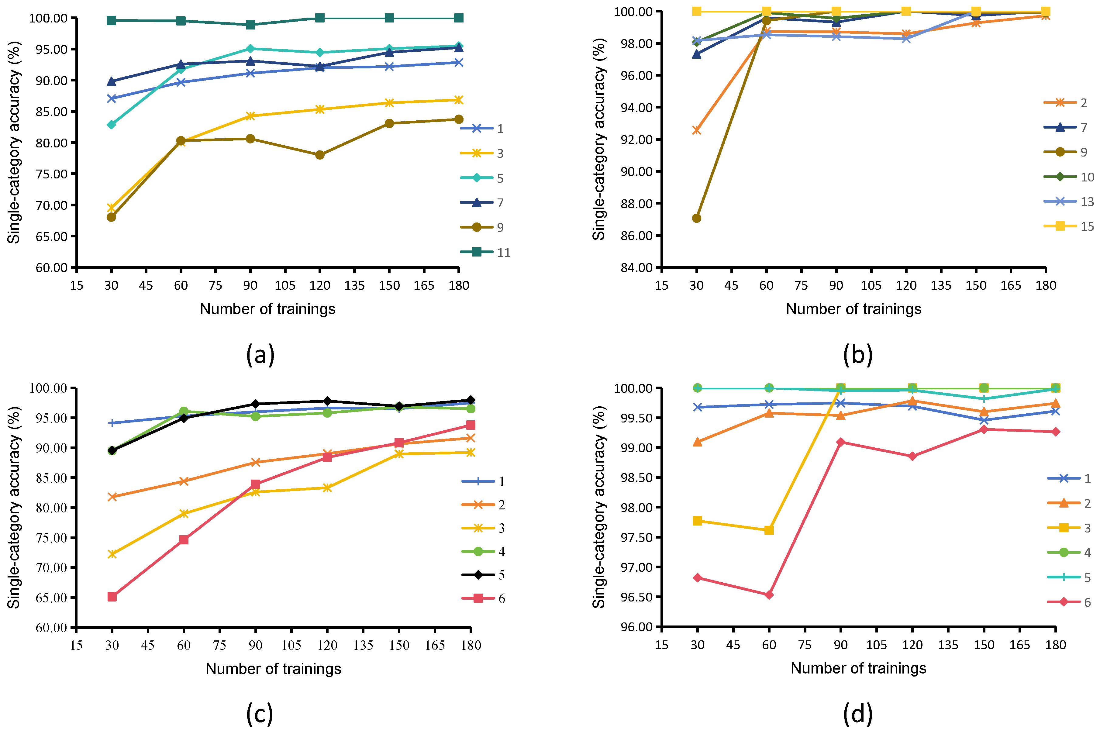
As shown in Figure 8, by analyzing the category-level accuracy of the four datasets, it was found that there is a significant difference in the effect of increasing the number of training samples on the accuracy of each category. In the MUUFL dataset, the accuracy for the Trees category increased from 87.06% to 92.86%, which is a flat increase, indicating that the model converged earlier on the learning of features in this category. The Grass Groundsurface category increased from 69.56% to 86.85%, which significantly benefited from the increase in the number of samples, reflecting the need for more data support for its complex texture. The Sidewalk category only increased from 68.04% to 83.73% but decreased in precision in the 90–120 sample interval, highlighting its classification challenges due to the spectral similarity of the materials. The Cloth Panels category consistently maintains nearly 100% precision, validating the strong separability of its unique spectra. In the Houston dataset, the easy-to-classify categories, such as Synthetic Grass and Water, reached an accuracy of over 99% at 30 samples, and the increase in samples had limited improvement in performance. In the Augsburg dataset, the accuracy of the Commercial Area category jumps from 65.14% to 93.79%, which indicates that the increase in samples effectively alleviates the problem of spectral mixing in urban functional areas. The accuracy for the Water category fluctuates greatly, limited by the spectral similarity between water bodies and shadows. The starting point of each category in the Trento dataset is over 96%, and the sample increase only brings a slight improvement of ≤0.5%, which confirms that its feature boundaries are clear and the spectral separation is high. Through category-level analysis, it can be concluded that the categories with unique spectral features, such as Cloth Panels and Synthetic Grass, are insensitive to the number of samples, and the categories with complex textures and spectral overlap, such as Grass Groundsurface and Commercial Area rely on sufficient samples to learn the features. When the sample size reaches 150, the accuracy of most of the categories stabilizes, and a further increase in sample size brings only ≤0.5% improvement. When the sample size reaches 150, the accuracy stabilizes, and the marginal benefit of further increasing the sample size decreases.

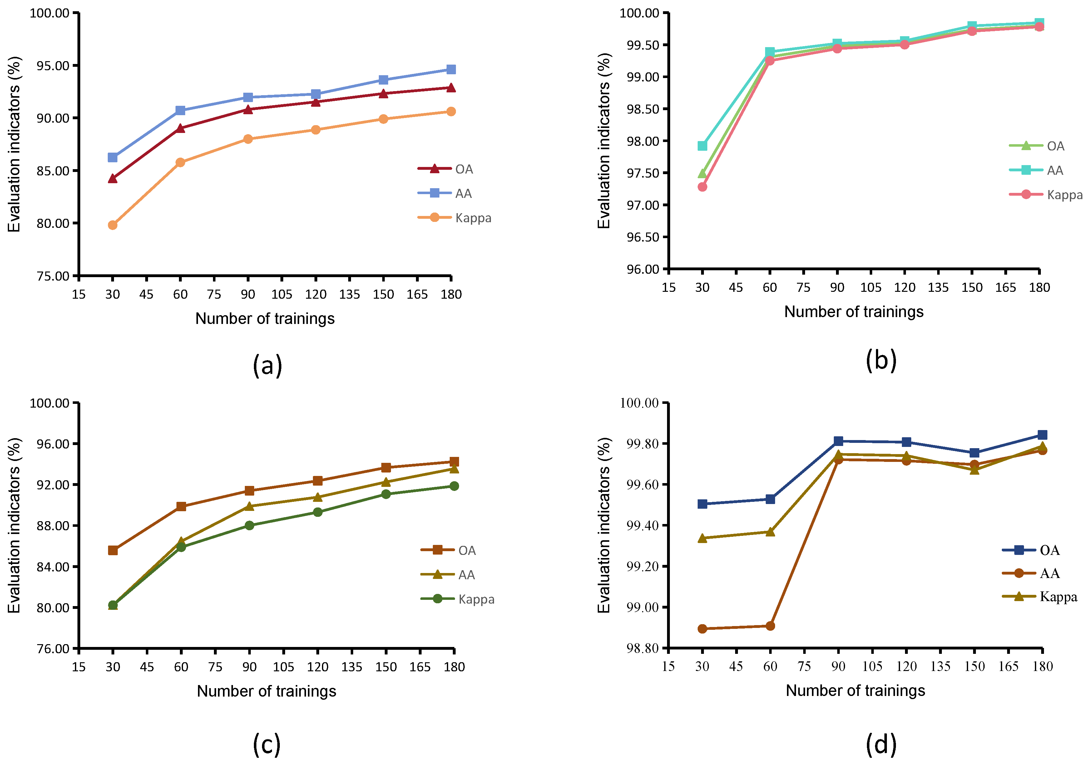
As shown in Figure 9, the overall metrics show a continuous upward trend with the increase in sample size, but the magnitude of gain and the speed of convergence vary significantly among different datasets: in terms of performance improvement, MUUFL’s OA increases from 84.25% to 92.88%, and Kappa increases from 79.80% to 90.61%, which is the largest increase, reflecting the underfitting caused by insufficient initial samples. Augsburg’s AA increased from 80.23% to 93.55%, indicating that the increase in training size effectively improves the ability to recognize a few categories. Houston and Trento show only limited improvement of ≤2.3% with the increase in samples due to the initial accuracy being higher than 97%. In terms of convergence characteristics, the OA, AA, and Kappa of all datasets plateau when the sample size reaches 150. The Kappa increase is generally higher than that of OA, which highlights the significant effect of sample increase on the improvement of category consistency. When the sample size was increased from 150 to 180, MUUFL’s OA only increased by 0.57%, verifying the cost-effectiveness of 150 samples. Augsburg’s OA reached 93.66% at 150 samples, which is close to the 94.24% at 180 samples, further supporting the utility of this sample size. In summary, increasing the training sample size to 150 can significantly improve model generalization ability, especially for the complex category of spectral–spatial mixing, but continuing to expand the sample size has diminishing returns. Therefore, the sample size should be reasonably selected to balance the classification performance and computational cost, which is suitable for remote sensing application scenarios with limited resources.

7. Conclusions

This study proposes CSTC, a dual-fusion network based on visual Transformers, for the collaborative classification of HSI and LiDAR data. The core innovation of CSTC lies in its dual-fusion mechanism: through a symmetric cross-attention module, it achieves deep interaction and dynamic alignment between HSI spectral features and LiDAR spatial elevation features, effectively addressing the shortcomings of traditional single-fusion or parallel-branch architectures in utilizing cross-modal complementary information. Secondly, the interacted features are spliced together and fed into the quadratic Transformer encoder for in-depth cross-modal semantic integration, which significantly strengthens the discriminative ability of features. Meanwhile, the model uses CCFF for HSI spatial–spectral fusion for modal characteristics and stacks MobileNetV2 for LiDAR spatial structure extraction, which effectively enhances the discriminative properties of intra-modal features. Extensive experiments on four classical benchmark datasets, namely MUUFL, Trento, Augsburg, and Houston, show that CSTC outperforms the existing state-of-the-art methods in terms of overall accuracy (OA), average accuracy (AA), and Kappa coefficients, and the ablation experiments further validate the dual-fusion mechanism and the effectiveness and synergies of each key module. The model achieves a good balance between training and inference efficiency while maintaining a reasonable parameter scale, showing strong potential for practicality. The core contribution of these results is demonstrating that fine-grained modal interaction and staged deep fusion are effective ways to solve the problem of effective fusion of HSI and LiDAR heterogeneous information and improve classification accuracy.

However, this study also has limitations, mainly because its validation is limited to standardized publicly available datasets. These datasets are usually preprocessed with relatively controllable noise and relatively static scenes. The robustness and generalization ability of the CSTC architecture in real-world complex scenes have not been fully validated. In addition, although the model is designed with lightweighting in mind, deployment efficiency on edge computing platforms with extreme resource constraints still needs to be optimized. Future work will focus on exploring the following directions: assessing the robustness of the model on real noisy environments and time-varying data, introducing remote sensing datasets containing complex noise and time-varying data for testing, and exploring corresponding robust training strategies; promoting the lightweighting of the model and investigating more efficient Transformer variants or knowledge distillation techniques to adapt to edge platforms such as UAVs and satellite payloads; and extending the model’s applicability by applying it to multi-temporal remote sensing data analysis or fusing more modalities for data collaborative classification tasks in order to cope with a wider range of remote sensing information interpretation needs.