Highlights
What are the main findings?
- The random forest (RF) classifier model, combined with an extensive reference dataset, yielded excellent results for mapping crop types in smallholder farms.
- All three seasonal crop maps in Thailand achieved an overall accuracy of more than 85%.
What is the implication of the main finding?
- The crop type classification maps highlighted sugarcane, rice, and cassava as the principal crops in the region.
Abstract
Accurate and timely information regarding the locations and types of crops cultivated is essential for sustainable agriculture and ensuring food security. However, accurately mapping season-specific crop types in tropical and subtropical regions is challenging due to smallholder farms, fragmented fields, predominant clouds, and limited seasonal reference data. To address these limitations, this study employed optical and radar satellite data in conjunction with machine learning algorithms, including Random Forest (RF), Support Vector Machine (SVM), and Gradient Tree Boosting (GBoost), utilizing a large number of reference datasets across crop seasons. To validate the results, extensive field visits were undertaken throughout the year. Our focus centered on two regions in Thailand recognized for their small fields and frequent overcast conditions. Utilizing over 8000 reference points, we mapped 12 crop types in Chaiyaphum province and 13 crop types in Suphan Buri province for three cropping seasons in 2023. The RF algorithm proved to be the most effective, demonstrating superior performance across all seasons in comparison to the other models, achieving an overall accuracy exceeding 85%, with classifications for sugarcane and rice exceeding 90%. The resultant maps identified sugarcane, rice, and cassava as the principal crops in the region. This research exemplifies a methodology for producing highly accurate seasonal crop maps, providing valuable tools for making informed decisions for crop sustainable management, thereby supporting sustainable agriculture practices. Our findings underscore the potential of Earth observation satellites and machine learning algorithms in addressing significant agricultural challenges and facilitating the development of more resilient strategies for food security.
1. Introduction
The agricultural landscape of Thailand represents a vibrant tapestry of richness and diversity, characterized by an extensive array of crops and distinctive farming practices [1]. Agriculture plays a fundamental role in Thailand’s economy, culture, and daily life, not only providing sustenance for the population but also enhancing the livelihoods of rural communities. Commonly referred to as the “rice bowl of Asia,” Thailand occupies a prestigious position as one of the world’s leading exporters of rice. Rice, serving as a staple in the local cuisine and a significant commodity in international trade, embodies the essence of the nation’s agricultural identity [2]. While numerous industrialized nations have transitioned away from small-scale farming, Thailand distinguishes itself through a considerable number of families that continue to manage their farms [3,4]. This harmonious amalgamation of traditional techniques and modern technology enhances the uniqueness of its agricultural system. Benefiting from its tropical climate and fertile soils, Thailand possesses optimal conditions for triple cropping. The nation cultivates a diverse range of crops, including rubber and sugarcane, as well as exotic fruits such as durians and mangosteens [5]. Beyond serving as a means of sustenance, agriculture in Thailand is profoundly intertwined with the nation’s heritage, which is celebrated through numerous festivals, rituals, and cherished traditions [6].
In the dynamic context of agriculture, the mapping of crop types is essential [7]. Timely and precise crop type maps provide critical insights into the geographical distribution of various crops, thereby enabling farmers, policymakers, and researchers to make informed decisions [8]. With the availability of precise crop maps, resources such as water and fertilizers can be managed more efficiently [9]. Furthermore, these maps assist in predicting and monitoring crop production, which is vital for addressing global food demands and confronting challenges such as climate change, pest infestations, and diseases [3]. Additionally, tracking crop sequences—patterns of crop rotation over time—proves invaluable for understanding soil health, land use, and sustainable farming practices [10]. The analysis of crop rotation mapping yields valuable information regarding how farmers can enhance nutrient management, mitigate risks from pests and diseases, and achieve improved yields.
Over the past five decades, remote sensing technology has experienced a substantial transformation, evolving from coarse-resolution imagery to high-resolution, multi-sensor, real-time monitoring capabilities [7,11,12,13]. This technology has facilitated numerous applications, including land cover mapping [14,15], tracking of invasive plant species [16], monitoring of deforestation and reforestation initiatives [17], and analysis of wetland ecosystems [18], thereby providing unprecedented insights. In the domain of agriculture, remote sensing data has fundamentally enhanced our understanding of crop types, growth patterns, distribution, and yield estimation [19,20,21]. Moreover, the integration of remote sensing with machine learning substantially increases its efficacy, as machine learning algorithms proficiently classify crops and monitor variations in land use [9,19,22,23,24,25].
Recently, the integration of multi-temporal data from various sensors, in conjunction with several machine learning algorithms, has demonstrated significant potential for mapping crop rotations. For example, Blickensdörfer et al. [8] classified 14 crop classes across Germany by utilizing a time series comprising Sentinel-1 (S1), Sentinel-2 (S2), and Landsat data, combined with a random forest (RF) classifier, achieving an overall accuracy (OA) exceeding 78%. Ghassemi et al. [26] produced European-wide crop maps considering 21 classes based on multi-temporal S2 and S1 data together with RF and support vector machine (SVM) with an accuracy of 78.%. Xing et al. [27] identified five crop rotations in Shandong Province, China, by employing a time series of S2 data and the RF, resulting in OAs of 93% and 85%. Qi et al. [28] produced four crop rotations in the Yellow River basin in China using a time series of S2 images and the machine learning algorithms, including one-class support vector machine (OC-SVM), decision trees (DTs), k-means clustering, and RF methods, achieving a high OA of over 95% across various seasons. Furthermore, Pott et al. [29] classified crop rotations on the South American map, particularly in Brazil, utilizing multi-temporal S1 and S2 datasets together with the RF, achieving an OA of 95%. These exemplary findings demonstrate both efficiency and reliability in the mapping of crop-type rotations. However, mapping crop type rotation across different seasons poses challenges attributable to cloud-corrupted optical satellite imagery, seasonal and phenological variations, diverse crop types, and the absence of reliable ground truth data. In addition, these machine learning algorithms, together with expensive ground data, have not yet been fully evaluated across different seasons within a year, especially in Thailand.
As discussed in the study conducted by Suwanlee et al. [30], some of the issues are addressed by advancements in remote sensing technology, e.g., through integration of data from S1, S2, Landsat, and ALOS satellites and several machine learning approaches (OC-SVM, DT, SVM, and RF) in mapping the annual sugarcane crop in the Northeast of Thailand. The combination of optical and radar imagery significantly enhances the OA, with a range of 80–94%. Valero et al. [31] mapped main crop types in three European test sites using the combined multi-temporal S1 and S2 datasets together with the RF classifier, achieving OA values of 80 to 90%. Jain et al. [32] monitored cropland in Arrah district, India, using very high SkySat imagery and a phenology-based index. Moreover, Suwanlee et al. [33] mapped crop types in the Northeast of Thailand using S1, S2, and the Highly Scalable Temporal Adaptive Reflectance Fusion Model (HISTARFM) data together with the RF classifier method, resulting in the OA exceeding 85%. Therefore, multi-temporal remote sensing data can effectively monitor intra- and inter-seasonal changes, such as planting and harvesting, thereby facilitating the improved mapping of diverse cropping systems, particularly in countries like Thailand. However, variations in crop growth cycles and farming methodologies contribute an additional layer of complexity. In regions characterized by mixed farming and small field sizes, cloud coverage makes crop identification particularly challenging due to similarities in spectral information and blurring/mixing effects at field boundaries.
Despite the progress in analytics and technology, gaps remain in accurately mapping season-specific crop types in mixed cropping systems, smallholder farms, and regions with cloudy conditions. Additionally, there is a lack of seasonal reference data and limited comprehensive methods for measuring optimal machine learning approaches, as seen in Thailand. In particular, season-specific crop mapping based on several machine learning models, combined with a large number of reference datasets across crop-growing seasons in Southeast Asian countries, has yet to be rigorously tested under conditions of high crop diversity and the complexity of cropping systems with mixed crops in small fields. To address these gaps, this study concentrates on mapping crop types and cropping patterns in Thailand with the following objectives:
- Classify season-specific crop types in smallholder farming regions of Thailand during the 2023–2024 period, leveraging multi-temporal data acquired from various Earth Observation (EO) sensors.
- Evaluate the effectiveness of machine learning algorithms, specifically RF, SVM, and gradient tree boosting (GBoost), for season-specific crop classification in mixed cropping systems based on an extensive collection of reference data.
- Analyze temporal changes in crop patterns across various seasons, July–October, November-February, and March-June, to identify crop sequences and cropping patterns.
In this way, the study provides up-to-date and precise mappings of season-specific crop types and cropping patterns for sustainable agricultural management in Thailand. The mapping of crop rotation enables local governments to organize cultivation activities, including those related to sugar mills, and lays the foundation for improved agricultural planning, enhanced crop understanding, and effective resource management across the region.
2. Study Area and Data
2.1. Study Area
The two selected study areas (Sentinel-2 tiles 47QRU and 47PNS) possess not only strategic significance but are also crucial vertices of agricultural prosperity, located in proximity to essential sugar mills and various agricultural industries (Figure 1). These regions are distinguished as vital hubs for both farming and production. The landscape exhibits remarkable variability, ranging from flat plains situated just 11 m above sea level to mountain peaks ascending to 1539 m, exemplifying the diversity of nature. The tropical semi-humid climate, categorized as Aw-main under the Köppen system, is exceptionally conducive to cultivation, encompassing three distinct seasons: an intensely hot summer from mid-February to mid-May, a fruitful rainy season from mid-May to mid-October, and a refreshing winter from mid-October to mid-February. The average temperature is 27 °C, with annual rainfall measuring 1690 mm and humidity levels persisting around 72%.
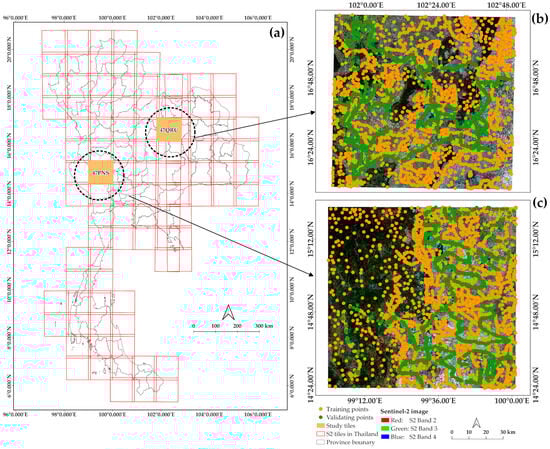
Figure 1.
Location of the two study areas in Thailand: (a) Sentinel-2 tiles 47QRU and 47PNS; (b) and (c) true color satellite imagery dated November 2023, along with reference points utilized for training (in orange), respectively, validation (in green).
The tributaries that traverse these landscapes provide a vital water supply for crops and sustain local communities. The favorable climate and rich geographical features render this region extraordinarily well-suited for farming. Farmers have adapted to these conditions, traditionally cultivating staple crops such as rice, sugarcane, cassava, and para rubber, employing time-honored agricultural practices to optimize yields. This exceptional combination of natural resources and agricultural expertise has nurtured and solidified the region’s reputation as a thriving hub for agricultural excellence.
2.2. Reference Data
Reference data were acquired during three significant growth periods: July 1–30, November 1–30, and January 8–30. Observations encompassed 12 crop types and land use classes in 47QRU, and 13 in 47PNS, representing a variety of land uses, including sugarcane, rice, rubber, cassava, and palm oil, among others (Table 1). For each period, we collected the ground truth in two rounds of fieldwork (the second week for the training model and the third and fourth weeks for map validation). In this study, eight people were separated into two groups for data collection using two cars. Moreover, the green dots, as shown in Figure 1, serve as validation and are aligned with the main roads due to their easy access and the recording of the sample datasets. A simple random sampling methodology was employed to ensure comprehensive coverage across the areas of interest (Figure 1). Data points were collected along the roads leading to the same fields across the three seasonal periods. Reference points were documented using a handheld Global Positioning System (GPS) device, a Garmin 62s, to ensure high precision. The data were segmented into training (90%) and validation (10%) sets, thereby maximizing the reliability of the classifier utilized. This methodology guaranteed robust and dependable map outputs.

Table 1.
Number of reference points collected during various crop seasons through fieldwork for the 12 (47QRU) and 13 (47PNS) dominant classes utilized for the classification of season-specific crop types in the 2023–2024 period. The number of classes differs across the two study regions, as the pineapple crop is not present in 47QRU.
2.3. Earth Observation (EO) Data
Between June 2023 and July 2024, we gathered multi-temporal data from two radar satellites (S1 and ALOS-2) and two optical satellites: S2 and Landsat 8/9 (Table 2). Among the optical imagery, we selected only images with less than 60% cloud cover. All EO data were processed using GEE [30]. In this study, the scene (47QRU or 47PNS tile) refers to all individual image granules covering the study area, not the number of unique acquisition dates.
Table 2.
Number of Sentinel-1, Sentinel-2, Landsat 8/9, and ALOS-2 in 2023–2024 for each study area and cropping period.
Regarding the S1 SAR data, Level-1 Ground Range Detected (GRD) images were utilized. These dual-polarization C-band images are accessible at a resolution of 10 m, and capture both VV (vertical-vertical) and VH (vertical-horizontal) polarizations. The preprocessing of all available S1 data involves noise removal, thermal noise removal, radiometric calibration, speckle filtering, terrain correction, and conversion from sigma0 to dB [30,34]. To enrich the S1 feature set, the VV/VH ratio and the Radar Vegetation Index (RVI) were added. All 267 S1 scenes were processed within the GEE framework [30].
The C-band imagery from S1 was complemented by L-band SAR data from ALOS-2, acquired in ScanSAR mode, which provides horizontal-horizontal (HH) and horizontal-vertical (HV) polarizations at a resolution of 25 m. A total of 109 ALOS-2 scenes were utilized, all of which underwent preprocessing by the Japan Aerospace Exploration Agency (JAXA) for orthorectification and topographic adjustments [35]. In GEE, digital numbers (DN) were converted to decibels (dB), followed by the application of noise reduction techniques utilizing a focal median filter, and the calculation of an HH/HV ratio for analytical purposes [36]. Using the nearest neighbor method, the 25 m pixels were subsequently resampled to 10 m to ensure compatibility with other datasets.
Within the optical part of the electromagnetic spectrum, we analyzed 1255 scenes from the S2 Level-2A Multispectral Instrument (MSI) data, which included four 10 m bands (B2, B3, B4, and B8) and six 20 m bands (B5, B6, B7, B8a, B11, and B12), the latter resampled to 10 m for consistency. Scenes exhibiting above 60% cloud cover were discarded using the Scene Classification (SCL) band in GEE to identify clouds and shadows [36].
To further complement the available optical data, an additional 233 images from Landsat 8 and Landsat 9 were incorporated, selecting spectral bands 2-7 at a resolution of 30 m. These images underwent atmospheric correction conducted by the United States Geological Survey (USGS) Earth Resources Observation and Science (EROS) Center. Cloud pixels were eliminated employing the CFmask procedure [37], which utilizes Quality Assessment (QA) data. Similar to the preceding datasets, these spectral bands were resampled to a 10 m resolution to align with the S2 data. By integrating data from S1, S2, ALOS-2, and Landsat 8/9, a comprehensive dataset was created that effectively maps crop types and patterns across the study area.
2.4. Vegetation Indices (VIs)
Following the resampling of the S2 and Landsat 8/9 datasets, a range of vegetation indices (VIs) was computed and appended to the existing dataset (Table 3). To further refine the analysis, the highest specific seasonal values of NDVI and GNDVI were extracted, e.g., maximum NDVI (MaxNDVI), maximum NDII (MaxNDII), and maximum GNDVI (MaxGNDVI).
Table 3.
Summary of vegetation indices (VIs) derived from multi-sensor data of S2 and L8/9. In these formulas, NIR refers to the near-infrared band, RED indicates the red band, BLUE represents the blue band, GREEN denotes the green band, and SWIR1 refers to the short-wave infrared band.
2.5. Pixel-Based Compositing and Auxiliary Data
To create seasonal composites, we employed several compositing methods (e.g., minimum, median, and maximum) [48,49]. This approach produces cloud-free synthetic images to facilitate the downstream classification task. In our study, we developed composite images corresponding to various time intervals—specifically, one, two, three, and six months. All spectral bands and VIs (S1, S2, Landsat, and ALOS) were processed in this way across the three seasons (e.g., Jul–Oct, Nov–Feb, and Mar–Jun).
To further facilitate the differentiation between crops, we also included gridded climate (temperature and rainfall) and elevation data. For climate data, we utilized a dataset comprising 30 years of average temperature and precipitation information sourced from WorldClim version 2 [50], which features a resolution of 1 km2. Elevation data were obtained from NASA’s Shuttle Radar Topography Mission (SRTM), which utilizes radar interferometry to provide a resolution of 30 m. All data were aligned with the 10 m S2 datasets.
3. Classification Procedures
This study aimed to map and track crop patterns across different seasons in two regions of Thailand: the S2 tile 47QRU in Chaiyaphum province and 47PNS in Suphan Buri province during the year 2023. To achieve this objective, we analyzed data from various optical and radar satellite resources, obtained and applied powerful machine learning methods using a large number of seasonal reference datasets from fieldwork. The methodology performed from the GEE platform comprises three main steps:
Data Preparation: Gathering and preparing time-series satellite data from various sensors.
Model Development: Creating and fine-tuning classification models.
Map Evaluation: Utilization of independent validation points (see Section 2.2 and Figure 1) for the assessment of map accuracy.
A training dataset of 8000 points was used to train the classifiers for each crop season. Three distinct machine-learning models were developed to classify crop patterns during the primary growing periods: July to October, November to February, and March to June. The workflow for this process is presented in Figure 2.
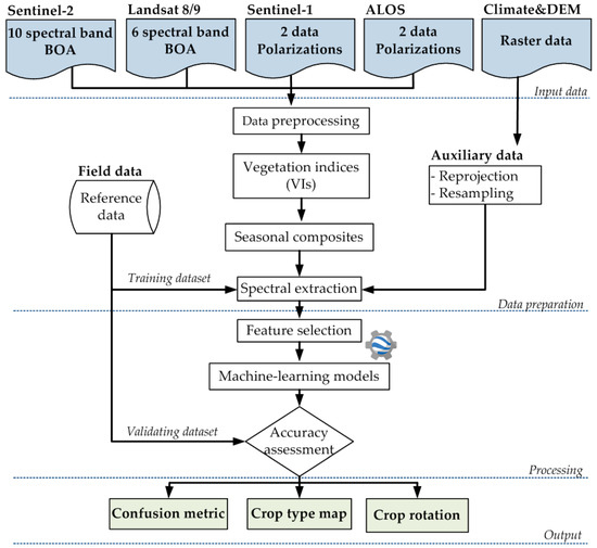
Figure 2.
Workflow used as the methodology for crop mapping in the two provinces of Thailand.
3.1. Feature Selection
This study employed the RF algorithm to identify the most significant features from the S1, S2, Landsat 8/9, and ALOS datasets to enhance the accuracy of classification models. Research conducted by Hossain and Chen [51] has consistently demonstrated that the emphasis on key features not only mitigates the risk of overfitting and conserves computational resources but also significantly enhances the accuracy of crop-type mapping. In the present study, a recursive feature selection method was implemented utilizing the Mean Decrease in Accuracy (MDA) technique, as introduced by Immitzer et al. [52], on the GEE platform, following recent findings by Som-ard et al. [10]. As a result, the optimized features for each seasonal predictive model were selected and used. In this study, the important features for each of the three seasons selected through this methodology were subsequently employed to construct each season’s predictive models.
3.2. Classification Algorithms
In this study, machine learning algorithms such as RF, GBoost, and SVM were integrated with a comprehensive reference dataset to effectively map season-specific crop types. RF is a robust and widely utilized machine learning technique designed for classification and regression tasks [53]. It operates by constructing an ensemble of decision trees, each trained on distinct subsets of the data. Collectively, these trees enhance final predictions, thereby increasing the accuracy of the model and minimizing the risk of overfitting [53]. The algorithm employs two essential parameters: (1) the number of trees (tree), which determines the quantity of decision trees generated; this study utilized between 50 and 500 (at the step interval of 50); and (2) random features per split, which specifies the number of features assessed for each tree split. In this study, we fit the number of trees to 500 trees for all three seasonal predictive models. This work established it as the square root of the number of features as recommended in Ghassemi et al. [26].
GBoost represents an alternative machine learning methodology that employs boosting techniques to improve performance by optimizing differentiable loss functions [54]. This algorithm has demonstrated exceptional proficiency in managing high-dimensional data and intricate patterns, thereby rendering it particularly suitable for remote sensing applications [55]. The primary parameters for GBoost encompass: (1) the number of trees, which regulates the quantity of iterations within the boosting process; (2) the loss function, which delineates the method by which errors are computed and minimized. In the course of this study, we conducted experiments concerning the number of trees, varying from 50 to 500 (at intervals of 50). The ideal value for the predictive models across all seasons was determined to be 500 trees, indicating that this number of trees yields the best results, thereby highlighting the model’s simplicity and efficiency within this context.
SVM is a versatile technique in machine learning dedicated to the classification of data through the maximization of separation among distinct groups within a high-dimensional space [56]. A critical consideration in implementing SVM involves selecting the kernel, which significantly affects how the algorithm maps data into this space. In the context of our research, we employed the Radial Basis Function (RBF) kernel. Two principal hyperparameters were meticulously tuned: (1) cost, evaluated within a range of 1 to 500 (the interval of 1); (2) gamma, investigated within the range of 1 to 10 (the step of 1). The optimal configurations in this work were determined to be a cost of 2 and a gamma value of 0.01 for all three seasonal models.
The performance of all predictive models was evaluated using the standard statistical metrics described in Section 3.3. Utilizing these optimized models and the salient features identified (Section 3.1), we predicted crop types across the entirety of the study area. The implementation of these classifiers in GEE facilitated efficient data processing, despite the inherent challenges posed by small field sizes and persistent cloud cover.
3.3. Accuracy Assessment
The accuracy of the outcomes derived from various classification models was evaluated employing four principal metrics: overall accuracy (OA), user’s accuracy (UA), producer’s accuracy (PA) [57], and the kappa coefficient (KC) [58], all based upon an independent validation dataset (Table 1). To enhance our understanding of the reliability of the estimated crop areas, the uncertainty was also quantified with a 95% confidence interval (CI) using a stratified assessment process, as proposed by Olofsson et al. [59].
3.4. Crop Rotation Identification
We employed the maps derived from the supervised classification models to examine the temporal changes in crop types within our research areas. To enhance our understanding of these changes, we used stacked bar charts to illustrate the percentage of each crop type per season across both study areas. Furthermore, crop transitions were illustrated via a Sankey diagram, which delineates the proportional changes in crops from one period to another. This visualization effectively conveys the flow and transformation of various crop types throughout the study periods, thus providing insights into crop rotation patterns and dynamics. Additionally, we presented detailed maps featuring zoomed-in comparison boxes, which enabled us to distinctly emphasize and compare the evolution of crop patterns across the three periods. This approach facilitated a deeper understanding of the seasonal dynamics of crop distribution.
4. Results
4.1. Comparative Evaluation of Machine Learning Algorithms
In our analysis, we identified the key features essential for crop type classification for each of the three crop seasons by leveraging the capabilities of the RF algorithm. Figure 3 shows the top important features for three seasons and two study regions. This process highlighted the ten most important features that emerged as critical in our study: the S2 bands around the NIR red-edge (B7, B6, and B8), the two S1 backscatter coefficients (VV and VH), ALOS HV, and specific Landsat bands (B6 and B7). These features enabled us to differentiate between various crop classes across the study area effectively. Notably, during the first (Jul–Oct) and second (Nov–Feb) growing periods, B7, B6, and B8 were associated with crop greenness, peak phenology, and rainfall patterns, while two S1 backscatter coefficients, VV and VH, corresponded to bare soil and newly planted crops for the third (Mar–Jun) period. It has, however, also to be noted that the selected features varied strongly between the two study sites and the three growing seasons (Figure 4).
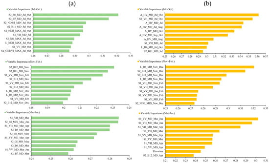
Figure 3.
Top ten key features for each cropping season as identified by the RF method classifying data using multi-modal and multi-temporal data over Thailand: (a) study area 47QRU, (b) study area 47PNS. The variable name is sensor type_band information_compositing methods (minimum: MIN; median: MD; maximum: MAX) month, for example: S2_B12_MD_Nov.

Figure 4.
This image shows how often a given feature is selected across the two study sites and three growing seasons. The minimum is one (white), the maximum is six (black), and various shades of gray represent between these values.
Table 4 presents the overall accuracy (OA) and Kappa coefficients (κ) for the mapping of crop types and land cover across the two study regions and three periods. RF consistently outperforms the other models across all periods and study regions, achieving OA values ranging from 87 to 92%. This demonstrates a strong overall performance in accurately mapping crop types and land cover with high reliability. Compared to RF, GBoost performs adequately in the earlier periods but experiences a significant decline in the Mar–Jun period. SVM shows the lowest overall accuracy, with OA values sometimes plummeting to as low as 66%. Only in the first growing period (Jul–Oct), SVM demonstrates a performance comparable to the two competing classifiers.
Table 4.
Overall accuracy (OA) and kappa coefficient (κ) based on independent validation and the different machine learning models for season-specific crop types.
Figure 5 presents a true-color PlanetScope image, along with the three competing land cover classifications. The maps generated using the RF model are characterized by reduced clutter and enhanced spatial consistency compared to those produced by GBoost and SVM classifiers. The map results from RF-classification models for both regions demonstrate superior capability in differentiating between “sugarcane” and “cassava”, respectively, “pineapple” (Figure 5). As a result, the optimized RF model has been selected for predicting crop type classes across the study regions.
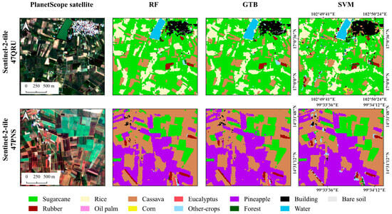
Figure 5.
Exemplary subsets of the maps produced by the three machine learning models, together with true color PlanetScope imagery, demonstrating an enhanced compactness and reduced clutter of the RF algorithm.
4.2. Crop Type Classification
The crop type and land cover classifications for the three growing seasons based on the RF classifier are shown in Figure 6. The maps depict the inter-seasonal crop distributions for three periods (i.e., July–October, November–February, and March–June) in 2023, providing critical insights into the spatial distribution of various crops across the three seasons and facilitating agricultural monitoring and management. The stable crop and land cover classes for the three growing seasons and the two study regions were as follows: rubber, oil palm, eucalyptus, pineapple, other crops, forest, buildings, and water. However, sugarcane, rice, cassava, corn, and bare soil have changed over three growing periods due to crop cultivation patterns and management in each season in Thailand. The dominant crop area changes were rice, sugarcane, and cassava, respectively, for the two study regions. Notably, the rice crop in 47QRU is the main change, with decreasing areas of 2318 km2, 0.12 km2, and 0.16 km2, while in 47PNS, the cultivated areas were reduced by 1030 km2, 317 km2, and 410 km2 for the three growing seasons. Moreover, sugarcane (47QRU) transformed the estimated areas to 3677 km2, 1960 km2, and 1875 km2, and the 47PNS tile with sugarcane crop areas appeared as 2049 km2, 1244 km2, and 1913 km2 for all growing seasons. The distributed crop areas across three growing seasons for the study regions are demonstrated in Figure 6.
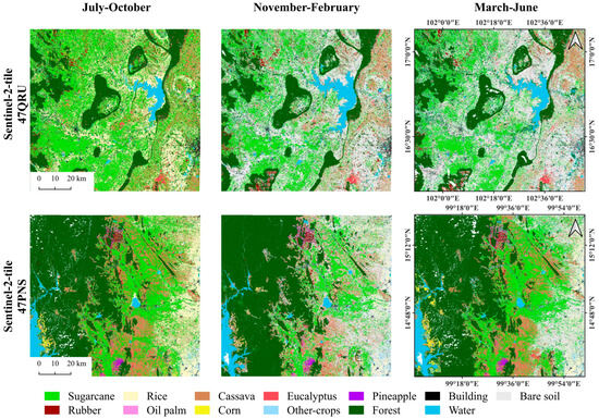
Figure 6.
Crop type maps for 47QRU and 47PNS tiles and the three growing seasons, obtained using the RF classifier models.
Figure 7 presents the confusion matrices derived from the validation datasets for each of the three crop seasons. It is noteworthy that the highest UA and PA values, exceeding 85%, were observed for nearly all crop types, particularly sugarcane, cassava, rubber, oil palm, and rice, across all crop seasons. The most significant misclassification was recorded in the “other crops” and “oil palm” classes, attributed to the substantial overlap of features.
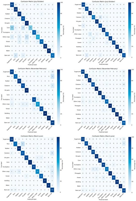
Figure 7.
Confusion matrices for both study areas and the three cropping seasons; (left) 47QRU, (right) 47PNS. The reported results refer to the RF classifier.
4.3. Crop Pattern Identification
Figure 8 shows the estimated and error-adjusted areas of crop types and LC classes with 95% CI for three cropping seasons between Jul and Oct, Nov and Feb, and Mar and Jun, for both study areas of S2 47QRU (a) and 47PNS (b) tiles, together with the best RF classification models.
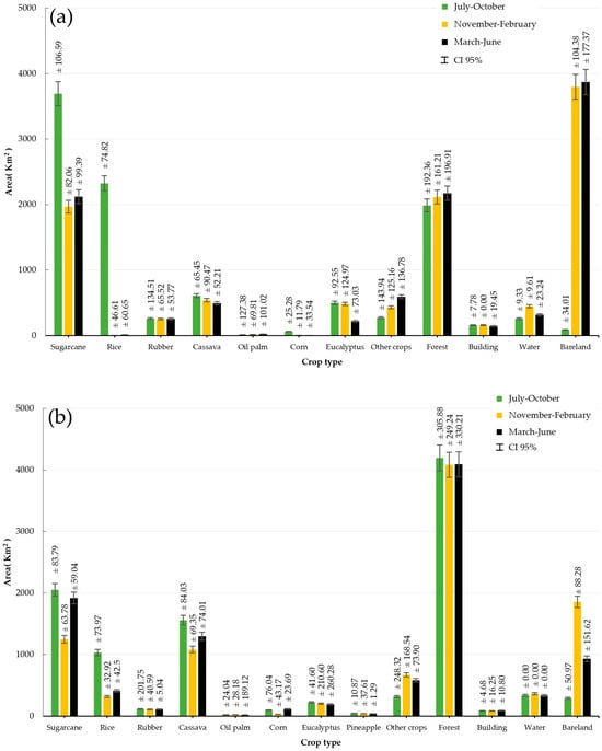
Figure 8.
The estimated crop types and land cover (LC) areas with 95% confidence interval (CI) for three cropping seasons between July and October, November and February, and March and June, for both study areas of S2 47QRU (a) and 47PNS (b) tiles, together with the optimized RF classification models.
According to Figure 8a, the primary cultivated crops were sugarcane, cassava, and rice. Conversely, during the Nov-Feb period, rice fields were not assessed, as they were not planted during this timeframe. Similarly, in Figure 8b, the most commonly cultivated crops remained sugarcane, cassava, and rice. A comparison of both study regions indicates that sugarcane maintained the highest proportion across all three periods, likely due to the proximity of sugarcane mills, which influence cultivation patterns. Over the three growing periods, the sugarcane crop is highly cultivated for both study regions, although the main seasons change in Thailand. It appears that farmers plant the sugarcane crop throughout the year, as it is the primary crop of the region. Cassava cultivation is similar to the sugarcane crop, and there are fewer plants in Jul–Oct due to an unsuitable season for the S2 47QRU region. During this period, farmers cultivate rice in some areas that were previously used for cassava crops. Conversely, the highly rice areas appeared in the rainy season (Jul–Oct) and decreased in the remaining seasons. Focusing on the Nov-Feb period, rice has not been planted in 47QRU due to the dry season. In contrast, rice fields in 47PNS, located in the central region of Thailand, exhibit three cropping patterns. The farmers in this region plant the rice crop throughout the entire year due to several factors, including sufficient water, effective crop management, accessibility, high yields per hectare, and proximity to industries.
Figure 9 illustrates the transitions in crop types and LC across the three seasons of 2023: Jul–Oct, Nov–Feb, and Mar–Jun. In Figure 9a, the most significant crop dynamics occurred between the Jul–Oct period and the Nov–Feb period, with a transition from sugarcane to bare soil and subsequently from bare soil to sugarcane between the Nov–Feb period and the Mar–Jun period. In Figure 9b, the most notable transitions occurred from rice to bare soil from the Jul–Oct period and the Nov–Feb period, and from bare soil to sugarcane from the Nov–Feb period and the Mar–Jun period. This information regarding changes in crop types is invaluable for understanding crop rotation patterns.
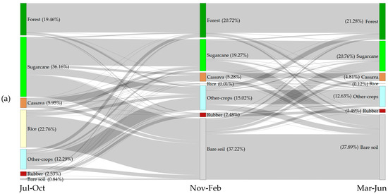
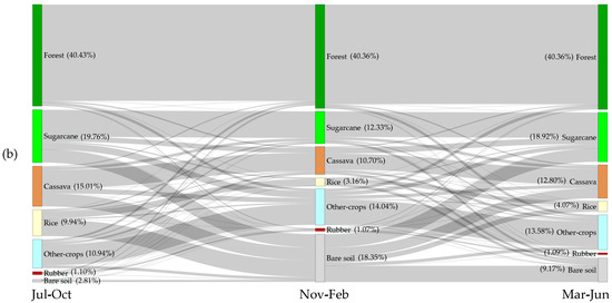
Figure 9.
Crop transition between July and October, November and February, and March and June, for both study areas of S2 47QRU (a) and 47PNS (b) tiles together with the optimized RF classification models.
According to Figure 9, well-defined transitions in crop types and land cover are observed across the crop-growing seasons. However, some implausible transitions appear between particular classes, such as “forest and other crops”, “rubber tree and forest”, and “other crops and sugarcane”. These inconsistencies are likely the result of misclassification for each growing season caused by spectral similarity and mixed pixels, leading to confusion between these crop types and land cover classes. However, this study confirms that analyzing cropping patterns and crop type transitions can provide valuable information for promoting sustainable agricultural practices, optimizing land use, and enhancing crop yield management.
5. Discussions
5.1. Evaluating the Potential of Machine Learning Algorithms
This study evaluated the effectiveness of three machine learning algorithms—RF, SVM, and GBoost—for season-specific crop type classification during the 2023–2024 period in mixed cropping systems with an abundance of smallholder farms. The experiments demonstrated that the RF model achieved the highest OA, exceeding 90%, and consistently outperformed the other tested algorithms. Our finding aligns with previous works [28,33] reinforcing the robustness of RF for crop type classification under conditions of small field sizes and complex landscapes. GBoost could not achieve the same performance as RF, but clearly outperformed the SVM classifier. The latter algorithm is known for requiring extensive fine-tuning to identify the optimal hyperparameters [30,60,61].
Despite these promising results, our analysis also found inconsistent and implausible results, for example, when labels transitioned back and forth between forest and crop classes. With an overall accuracy of around 90%, such inconsistencies are to be expected and warrant the development of methods directly classifying crop rotation patterns [25,26]. This study utilized a large number of reference points for all three seasons, thereby enhancing the model’s performance. However, this is time-consuming and resource-intensive. This may restrict the scalability of the approach in broader applications. Future work should also consider semi-automated labeling, transfer learning, or the use of open-access and ancillary datasets to reduce field data demands while maintaining reliable performance.
Based on the feature importance analysis, our experiments identified the most important variables for crop classification: S2 spectral bands B6, B7, and B8 along the NIR red-edge; S1 VV and VH backscatter coefficients, ALOS HV polarization, and two Landsat bands (B6 and B7). These features consistently contributed to distinguishing among crop types [62]. This finding aligns with prior studies [10,19,30], which also emphasized the effectiveness of these variables in distinguishing crops with overlapping spectral signatures.
Compared to GBoost and SVM, the classification results using the RF model showed greater smoothness and enhanced spatial consistency. The RF model exhibits reduced noise and demonstrates superior capability in differentiating between crop classes, notably between “sugarcane” and “cassava” as well as “sugarcane” and “pineapple”. The findings align with previous research [10], which highlights that the RF well classified the classes of “sugarcane” and “cassava” in a small field size (<1 ha) within a large region in Thailand. Although the RF classifier in this study demonstrated high flexibility and excellent performance, small fields containing mixed tree species still exhibited noise and mixed pixels. Future work could address these challenges by incorporating higher-resolution datasets (e.g., THEOS-2, PlanetScope, and AlphaEarth imagery), applying object-based image analysis (OBIA), integrating texture and landscape metrics, and exploring deep neural network (DNN) algorithms to capture spatial context better. These strategies may help mitigate spatial heterogeneity and further improve classification performance in complex agricultural landscapes.
As a result, the optimized RF model has been selected for predicting crop type classes across the study regions. Following suggestions by Suwanlee et al. [30], season-specific crop type maps were generated. Amongst the three cropping seasons, the highest accuracy was achieved during the period of Mar-Jun. This improved performance is primarily attributed to the greater availability of satellite sensor datasets and the more balanced distribution of reference samples across crop classes in both study regions. Conversely, the lower classification accuracy observed in the first period (Jul–Oct) is likely due to the substantial overlap in spectral signatures and similar levels of vegetation greenness among crop types [27,28,29,63]. Despite these challenges, the seasonal crop classification maps provide valuable insights into the spatial distribution of major crops throughout the year, supporting more effective agricultural monitoring, planning, and decision-making.
This study developed efficient RF predictive models, achieving high accuracy in crop type and LC classifications. However, some misclassifications persisted in each growing season due to spectral similarity and mixed pixels, causing confusion between certain crop types and LC classes. Future studies could address these issues by incorporating soft classification and deep learning approaches to capture spectral heterogeneity better and reduce boundary misclassification errors, as demonstrated in recent studies [64,65].
5.2. Crop Type Rotations
To the best of our knowledge, this is the first study in Thailand to successfully identify crop type rotations across three distinct agricultural seasons within areas characterized by small field sizes and complex landscapes. Our workflow effectively monitored and mapped the spatial distribution patterns of crop types over three seasons, demonstrating the feasibility and potential of multi-seasonal crop classification in a challenging agricultural environment.
The three individually produced crop type maps revealed a complex pattern of crop distribution, with rice, sugarcane, and cassava being the dominant crops. The subsequent analysis of crop sequences has identified several common rotations, including rice-sugarcane, rice-cassava, and sugarcane-cassava. Each crop possesses distinct characteristics that influence soil health, water usage, and economic viability, thereby significantly affecting agricultural sustainability and food security [66]. For example, residues from rice crops can enhance soil nutrient levels, benefiting subsequent crops such as cassava, which has been documented to demonstrate improved yields when cultivated after rice due to the nutrient recycling effect [67]. One key observation was the rotation of upland rice with sugarcane, a practice that can disrupt the life cycles of soil-borne pathogens, potentially reducing the risk of disease outbreaks [68]. From an economic perspective, market demands and government policies can influence the selection between these crops. In certain regions, sugarcane has been favored due to its higher profitability compared to rice, particularly when supported by low-interest credit and harvesting services [67,68,69]. Nevertheless, although sugarcane may offer superior economic returns, the cultivation of cassava by smallholders has been found to drive more robust local economic growth compared to sugarcane. The implications of altering crop types are complex and interconnected. Decisions regarding crop rotation and type must consider agronomic benefits, economic viability, environmental sustainability, and the impact of climate change. Policymakers and farmers should consider these factors to promote sustainable agricultural practices that support food security and ecological health.
Although this study provided valuable information on the transitions in crop types and LC across the three seasons of 2023: Jul-Oct, Nov-Feb, and Mar-Jun, some implausible changes were observed between classes, such as ‘forest and other crops’, ‘rubber tree and forest’, and ‘other crops and sugarcane’. Future work could reduce these errors by applying spatiotemporal filtering or object-based post-processing to remove unlikely changes before rotation analysis.
6. Conclusions
This study successfully mapped and monitored seasonal crop types in smallholder farms (<1 ha), fragmented fields, and cloudy regions in Thailand using a large number of seasonal reference data points and several machine learning algorithms (i.e., Random Forest (RF), Support Vector Machine (SVM), and Gradient Tree Boosting (GBoost)). In our results, the RF algorithm proved to be the most effective, demonstrating superior performance across all seasons compared to the other models, achieving an overall accuracy of over 85%. This study exemplifies a methodology for producing highly accurate seasonal crop maps, providing valuable tools for making informed decisions for crop sustainable management. Our findings possess significant implications for agricultural monitoring and policymaking for related stakeholders. This study has the potential to support initiatives aimed at enhancing food security, optimizing irrigation management, and guiding sustainable land use planning by providing accurate high-resolution maps of crop types and crop sequences in an area characterized by three distinct cropping periods. The results of this study can be utilized to develop decision-support tools for farmers, policymakers, and other stakeholders, thereby equipping them with valuable insights to improve crop yields and minimize environmental impact. The approach employed in this study could also be applied to different regions and countries, yielding valuable insights into agricultural development and food security. Future research should consider exploring the integration of additional data sources, such as a foundation model [70] that includes meteorological datasets and socio-economic factors, to attain a better understanding of the drivers of cropping decisions and to further enhance the map quality. Furthermore, the combination of deep learning techniques such as DNN or TempCNN with the existing methodology could enhance feature extraction and classification accuracy, particularly in diverse landscapes. This work underscores the potential of Earth observation satellites and machine learning algorithms in addressing significant agricultural challenges and facilitating the development of more resilient strategies for food security.
Author Contributions
Conceptualization, J.S.-a., M.D.H., S.K., S.R.S. and E.I.-V.; methodology, J.S.-a., M.D.H. and S.K.; software, J.S.-a. and S.K.; validation, J.S.-a. and V.V.; formal analysis, J.S.-a., S.K. and S.R.S.; investigation, J.S.-a., S.K. and S.R.S.; resources, J.S.-a.; data curation, J.S.-a., S.K. and S.R.S.; writing—original draft preparation, J.S.-a., M.D.H., V.V., A.P., E.I.-V., M.I. and C.A.; writing—review and editing, J.S.-a., M.D.H., S.R.S., V.V., P.H., A.P., E.I.-V., M.I. and C.A.; visualization, J.S.-a., S.K., S.R.S. and V.V.; supervision, J.S.-a.; project administration, J.S.-a.; funding acquisition, J.S.-a. All authors have read and agreed to the published version of the manuscript.
Funding
This research project was financially supported by Mahasarakham University.
Data Availability Statement
The data presented in this study are available on request from the corresponding author.
Conflicts of Interest
Author V.V., P. H. and A.P. was employed by the company Mitr Phol Sugarcane Research Center Co., LTD. The remaining authors declare that the research was conducted in the absence of any commercial or financial relationships that could be construed as a potential conflict of interest.
References
- Apipoonyanon, C.; Szabo, S.; Tsusaka, T.W.; Leeson, K.; Gunawan, E.; Kuwornu, J.K. Socio-economic and environmental barriers to increased agricultural production: New evidence from central Thailand. Outlook Agric. 2021, 50, 178–187. [Google Scholar] [CrossRef]
- Waqas, M.; Naseem, A.; Humphries, U.W.; Hlaing, P.T.; Shoaib, M.; Hashim, S. A comprehensive review of the impacts of climate change on agriculture in Thailand. Farming Syst. 2025, 3, 100114. [Google Scholar] [CrossRef]
- Yodkhum, S.; Gheewala, S.H.; Sampattagul, S. Life cycle GHG evaluation of organic rice production in northern Thailand. J. Environ. Manag. 2017, 196, 217–223. [Google Scholar] [CrossRef]
- Som-ard, J. Rice Security Assessment Using Geo-Spatial Analysis. Int. J. Geoinform. 2021, 16, 21–38. [Google Scholar]
- Romruen, O.; Karbowiak, T.; Tongdeesoontorn, W.; Shiekh, K.A.; Rawdkuen, S. Extraction and characterization of cellulose from agricultural by-products of Chiang Rai Province, Thailand. Polymers 2022, 14, 1830. [Google Scholar] [CrossRef]
- Liao, X.; Nguyen, T.; Sasaki, N. Use of the knowledge, attitude, and practice (KAP) model to examine sustainable agriculture in Thailand. Reg. Sustain. 2022, 3, 41–52. [Google Scholar] [CrossRef]
- Atzberger, C. Advances in remote sensing of agriculture: Context description, existing operational monitoring systems and major information needs. Remote Sens. 2013, 5, 949–981. [Google Scholar] [CrossRef]
- Blickensdörfer, L.; Schwieder, M.; Pflugmacher, D.; Nendel, C.; Erasmi, S.; Hostert, P. Mapping of crop types and crop sequences with combined time series of Sentinel-1, Sentinel-2 and Landsat 8 data for Germany. Remote Sens. Environ. 2022, 269, 112831. [Google Scholar] [CrossRef]
- Tariq, A.; Yan, J.; Gagnon, A.S.; Riaz Khan, M.; Mumtaz, F. Mapping of cropland, cropping patterns and crop types by combining optical remote sensing images with decision tree classifier and random forest. Geo-Spat. Inf. Sci. 2023, 26, 302–320. [Google Scholar] [CrossRef]
- Som-ard, J.; Immitzer, M.; Vuolo, F.; Ninsawat, S.; Atzberger, C. Mapping of crop types in 1989, 1999, 2009 and 2019 to assess major land cover trends of the Udon Thani Province, Thailand. Comput. Electron. Agric. 2022, 198, 107083. [Google Scholar] [CrossRef]
- Weiss, M.; Jacob, F.; Duveiller, G. Remote sensing for agricultural applications: A meta-review. Remote Sens. Environ. 2020, 236, 111402. [Google Scholar] [CrossRef]
- Zhang, Z.; Shu, D.; Liao, C.; Liu, C.; Zhao, Y.; Wang, R.; Huang, X.; Zhang, M.; Gong, J. FlexiSAM: A flexible SAM-based semantic segmentation model for land cover classification using high-resolution multimodal remote sensing imagery. ISPRS J. Photogramm. Remote Sens. 2025, 227, 594–612. [Google Scholar] [CrossRef]
- Aires, U.R.; Martins, V.S.; Ferreira, L.B.; Huang, Y.; Heintzman, L.; Ouyang, Y. Impact of sampling techniques on crop type mapping using multi-temporal composites from Harmonized Landsat-Sentinel images. Comput. Electron. Agric. 2025, 237, 110676. [Google Scholar] [CrossRef]
- Calderón-Loor, M.; Hadjikakou, M.; Bryan, B.A. High-resolution wall-to-wall land-cover mapping and land change assessment for Australia from 1985 to 2015. Remote Sens. Environ. 2021, 252, 112148. [Google Scholar] [CrossRef]
- Suwanlee, S.R.; Keawsomsee, S.; Pengjunsang, M.; Homtong, N.; Prakobya, A.; Borgogno-Mondino, E.; Sarvia, F.; Som-ard, J. Monitoring Agricultural Land and Land Cover Change from 2001–2021 of the Chi River Basin, Thailand Using Multi-Temporal Landsat Data Based on Google Earth Engine. Remote Sens. 2023, 15, 4339. [Google Scholar] [CrossRef]
- Pan, L.; Xia, H.; Zhao, X.; Guo, Y.; Qin, Y. Mapping winter crops using a phenology algorithm, time-series Sentinel-2 and Landsat-7/8 images, and Google Earth Engine. Remote Sens. 2021, 13, 2510. [Google Scholar] [CrossRef]
- Maqsood, M.H.; Mumtaz, R.; Khan, M.A. Deforestation detection and reforestation potential due to natural disasters—A case study of floods. Remote Sens. Appl. Soc. Environ. 2024, 34, 101188. [Google Scholar] [CrossRef]
- Pande-Chhetri, R.; Abd-Elrahman, A.; Liu, T.; Morton, J.; Wilhelm, V.L. Object-based classification of wetland vegetation using very high-resolution unmanned air system imagery. Eur. J. Remote Sens. 2017, 50, 564–576. [Google Scholar] [CrossRef]
- Pflugmacher, D.; Rabe, A.; Peters, M.; Hostert, P. Mapping pan-European land cover using Landsat spectral-temporal metrics and the European LUCAS survey. Remote Sens. Environ. 2019, 221, 583–595. [Google Scholar] [CrossRef]
- Zhang, S.; Qin, H.; Li, X.; Zhang, M.; Yao, W.; Lyu, X.; Jiang, H. Sensitive Multispectral Variable Screening Method and Yield Prediction Models for Sugarcane Based on Gray Relational Analysis and Correlation Analysis. Remote Sens. 2025, 17, 2055. [Google Scholar] [CrossRef]
- Raza, A.; Shahid, M.A.; Zaman, M.; Miao, Y.; Huang, Y.; Safdar, M.; Maqbool, S.; Muhammad, N.E. Improving Wheat Yield Prediction with Multi-Source Remote Sensing Data and Machine Learning in Arid Regions. Remote Sens. 2025, 17, 774. [Google Scholar] [CrossRef]
- Teixeira Pinto, C.; Jing, X.; Leigh, L. Evaluation analysis of Landsat level-1 and level-2 data products using in situ measurements. Remote Sens. 2020, 12, 2597. [Google Scholar] [CrossRef]
- Wang, J.; Xiao, X.; Liu, L.; Wu, X.; Qin, Y.; Steiner, J.L.; Dong, J. Mapping sugarcane plantation dynamics in Guangxi, China, by time series Sentinel-1, Sentinel-2 and Landsat images. Remote Sens. Environ. 2020, 247, 111951. [Google Scholar] [CrossRef]
- Wang, M.; Liu, Z.; Baig, M.H.A.; Wang, Y.; Li, Y.; Chen, Y. Mapping sugarcane in complex landscapes by integrating multi-temporal Sentinel-2 images and machine learning algorithms. Land Use Policy 2019, 88, 104190. [Google Scholar] [CrossRef]
- Wang, X.; Fang, S.; Yang, Y.; Du, J.; Wu, H. A New Method for Crop Type Mapping at the Regional Scale Using Multi-Source and Multi-Temporal Sentinel Imagery. Remote Sens. 2023, 15, 2466. [Google Scholar] [CrossRef]
- Ghassemi, B.; Dujakovic, A.; Żółtak, M.; Immitzer, M.; Atzberger, C.; Vuolo, F. Designing a European-wide crop type mapping approach based on machine learning algorithms using LUCAS field survey and Sentinel-2 data. Remote Sens. 2022, 14, 541. [Google Scholar] [CrossRef]
- Xing, H.; Chen, B.; Lu, M. A sub-seasonal crop information identification framework for crop rotation mapping in smallholder farming areas with time series sentinel-2 imagery. Remote Sens. 2022, 14, 6280. [Google Scholar] [CrossRef]
- Qi, H.; Qian, X.; Shang, S.; Wan, H. Multi-year mapping of cropping systems in regions with smallholder farms from Sentinel-2 images in Google Earth engine. GIScience Remote Sens. 2024, 61, 2309843. [Google Scholar] [CrossRef]
- Pott, L.P.; Amado, T.J.C.; Schwalbert, R.A.; Corassa, G.M.; Ciampitti, I.A. Mapping crop rotation by satellite-based data fusion in Southern Brazil. Comput. Electron. Agric. 2023, 211, 107958. [Google Scholar] [CrossRef]
- Suwanlee, S.R.; Keawsomsee, S.; Izquierdo-Verdiguier, E.; Som-Ard, J.; Moreno-Martinez, A.; Veerachit, V.; Polpinij, J.; Rattanasuteerakul, K. Mapping sugarcane plantations in Northeast Thailand using multi-temporal data from multi-sensors and machine-learning algorithms. Big Earth Data 2025, 9, 187–216. [Google Scholar] [CrossRef]
- Valero, S.; Arnaud, L.; Planells, M.; Ceschia, E. Synergy of Sentinel-1 and Sentinel-2 imagery for early seasonal agricultural crop mapping. Remote Sens. 2021, 13, 4891. [Google Scholar] [CrossRef]
- Jain, M.; Srivastava, A.K.; Joon, R.K.; McDonald, A.; Royal, K.; Lisaius, M.C.; Lobell, D.B. Mapping smallholder wheat yields and sowing dates using micro-satellite data. Remote Sens. 2016, 8, 860. [Google Scholar] [CrossRef]
- Suwanlee, S.R.; Keawsomsee, S.; Izquierdo-Verdiguier, E.; Moreno-Martínez, Á.; Ninsawat, S.; Som-ard, J. Synergistic use of multi-sensor satellite data for mapping crop types and land cover dynamics from 2021 to 2023 in Northeast Thailand. Int. J. Appl. Earth Obs. Geoinf. 2025, 141, 104673. [Google Scholar] [CrossRef]
- Filipponi, F. Sentinel-1 GRD preprocessing workflow. In Proceedings of the 3rd International Electronic Conference on Remote Sensing, online, 22 May–5 June 2019; p. 11. [Google Scholar]
- Shimada, M.; Itoh, T.; Motooka, T.; Watanabe, M.; Shiraishi, T.; Thapa, R.; Lucas, R. New global forest/non-forest maps from ALOS PALSAR data (2007–2010). Remote Sens. Environ. 2014, 155, 13–31. [Google Scholar] [CrossRef]
- Weigand, M.; Staab, J.; Wurm, M.; Taubenböck, H. Spatial and semantic effects of LUCAS samples on fully automated land use/land cover classification in high-resolution Sentinel-2 data. Int. J. Appl. Earth Obs. Geoinf. 2020, 88, 102065. [Google Scholar] [CrossRef]
- Skakun, S.; Wevers, J.; Brockmann, C.; Doxani, G.; Aleksandrov, M.; Batič, M.; Frantz, D.; Gascon, F.; Gómez-Chova, L.; Hagolle, O. Cloud Mask Intercomparison eXercise (CMIX): An evaluation of cloud masking algorithms for Landsat 8 and Sentinel-2. Remote Sens. Environ. 2022, 274, 112990. [Google Scholar] [CrossRef]
- Tucker, C.J. Red and photographic infrared linear combinations for monitoring vegetation. Remote Sens. Environ. 1979, 8, 127–150. [Google Scholar] [CrossRef]
- Cihlar, J.; Manak, D.; D’Iorio, M. Evaluation of compositing algorithms for AVHRR data over land. IEEE Trans. Geosci. Remote Sens. 2002, 32, 427–437. [Google Scholar] [CrossRef]
- Gitelson, A.A.; Kaufman, Y.J.; Merzlyak, M.N. Use of a green channel in remote sensing of global vegetation from EOS-MODIS. Remote Sens. Environ. 1996, 58, 289–298. [Google Scholar] [CrossRef]
- Gitelson, A.A.; Kaufman, Y.J.; Stark, R.; Rundquist, D. Novel algorithms for remote estimation of vegetation fraction. Remote Sens. Environ. 2002, 80, 76–87. [Google Scholar] [CrossRef]
- Le Maire, G.; François, C.; Dufrene, E. Towards universal broad leaf chlorophyll indices using PROSPECT simulated database and hyperspectral reflectance measurements. Remote Sens. Environ. 2004, 89, 1–28. [Google Scholar] [CrossRef]
- Yan, K.; Gao, S.; Chi, H.; Qi, J.; Song, W.; Tong, Y.; Mu, X.; Yan, G. Evaluation of the vegetation-index-based dimidiate pixel model for fractional vegetation cover estimation. IEEE Trans. Geosci. Remote Sens. 2021, 60, 4400514. [Google Scholar] [CrossRef]
- Huete, A.R. A soil-adjusted vegetation index (SAVI). Remote Sens. Environ. 1988, 25, 295–309. [Google Scholar] [CrossRef]
- Klemas, V.; Smart, R. The influence of soil salinity, growth form, and leaf moisture on-the spectral radiance of. Photogramm. Eng. Remote Sens 1983, 49, 77–83. [Google Scholar]
- Huete, A.; Didan, K.; Miura, T.; Rodriguez, E.P.; Gao, X.; Ferreira, L.G. Overview of the radiometric and biophysical performance of the MODIS vegetation indices. Remote Sens. Environ. 2002, 83, 195–213. [Google Scholar] [CrossRef]
- Serrano, L.; Ustin, S.L.; Roberts, D.A.; Gamon, J.A.; Penuelas, J. Deriving water content of chaparral vegetation from AVIRIS data. Remote Sens. Environ. 2000, 74, 570–581. [Google Scholar] [CrossRef]
- Griffiths, P.; van der Linden, S.; Kuemmerle, T.; Hostert, P. A pixel-based Landsat compositing algorithm for large area land cover mapping. IEEE J. Sel. Top. Appl. Earth Obs. Remote Sens. 2013, 6, 2088–2101. [Google Scholar] [CrossRef]
- Griffiths, P.; Nendel, C.; Hostert, P. Intra-annual reflectance composites from Sentinel-2 and Landsat for national-scale crop and land cover mapping. Remote Sens. Environ. 2019, 220, 135–151. [Google Scholar] [CrossRef]
- Garmaev, E.Z.; P’yankov, S.; Shikhov, A.; Ayurzhanaev, A.; Sodnomov, B.; Abdullin, R.; Tsydypov, B.; Andreev, S.; Chernykh, V. Mapping modern climate change in the Selenga river basin. Russ. Meteorol. Hydrol. 2022, 47, 113–122. [Google Scholar] [CrossRef]
- Hossain, M.D.; Chen, D. Performance comparison of deep learning (DL)-based tabular models for building mapping using high-resolution red, green, and blue imagery and the geographic object-based image analysis framework. Remote Sens. 2024, 16, 878. [Google Scholar] [CrossRef]
- Immitzer, M.; Neuwirth, M.; Böck, S.; Brenner, H.; Vuolo, F.; Atzberger, C. Optimal input features for tree species classification in Central Europe based on multi-temporal Sentinel-2 data. Remote Sens. 2019, 11, 2599. [Google Scholar] [CrossRef]
- Breiman, L. Random forests. Mach. Learn. 2001, 45, 5–32. [Google Scholar] [CrossRef]
- Friedman, J.H. Greedy function approximation: A gradient boosting machine. Ann. Stat. 2001, 29, 1189–1232. [Google Scholar] [CrossRef]
- Bailly, J.-S.; Arnaud, M.; Puech, C. Boosting: A classification method for remote sensing. Int. J. Remote Sens. 2007, 28, 1687–1710. [Google Scholar] [CrossRef]
- Vapnik, V.N. An overview of statistical learning theory. IEEE Trans. Neural Netw. 1999, 10, 988–999. [Google Scholar] [CrossRef] [PubMed]
- Congalton, R.G.; Green, K. Assessing the Accuracy of Remotely Sensed Data: Principles and Practices; CRC Press: Boca Raton, FL, USA, 2019. [Google Scholar]
- Pontius Jr, R.G.; Millones, M. Death to Kappa: Birth of quantity disagreement and allocation disagreement for accuracy assessment. Int. J. Remote Sens. 2011, 32, 4407–4429. [Google Scholar] [CrossRef]
- Olofsson, P.; Foody, G.M.; Stehman, S.V.; Woodcock, C.E. Making better use of accuracy data in land change studies: Estimating accuracy and area and quantifying uncertainty using stratified estimation. Remote Sens. Environ. 2013, 129, 122–131. [Google Scholar] [CrossRef]
- Zheng, Y.; Dong, W.; Lu, Y.; Zhang, X.; Dong, Y.; Sun, F. A new attention-based deep metric model for crop type mapping in complex agricultural landscapes using multisource remote sensing data. Int. J. Appl. Earth Obs. Geoinf. 2024, 134, 104204. [Google Scholar] [CrossRef]
- Suwanlee, S.R.; Qaisrani, Z.N.; Som-ard, J.; Keawsomsee, S.; Kasa, K.; Nuthammachot, N.; Kaewplang, S.; Ninsawat, S.; Mondino, E.B.; De Petris, S. Integrating PRISMA hyperspectral data with Sentinel-1, Sentinel-2 and Landsat data for mapping crop types and land cover in northeast Thailand. Egypt. J. Remote Sens. Space Sci. 2025, 28, 252–260. [Google Scholar] [CrossRef]
- Costa, J.d.S.; Liesenberg, V.; Schimalski, M.B.; Sousa, R.V.d.; Biffi, L.J.; Gomes, A.R.; Neto, S.L.R.; Mitishita, E.; Bispo, P.d.C. Benefits of combining ALOS/PALSAR-2 and Sentinel-2A data in the classification of land cover classes in the Santa Catarina southern Plateau. Remote Sens. 2021, 13, 229. [Google Scholar] [CrossRef]
- Yan, S.; Yao, X.; Zhu, D.; Liu, D.; Zhang, L.; Yu, G.; Gao, B.; Yang, J.; Yun, W. Large-scale crop mapping from multi-source optical satellite imageries using machine learning with discrete grids. Int. J. Appl. Earth Obs. Geoinf. 2021, 103, 102485. [Google Scholar] [CrossRef]
- Rana, S.; Gerbino, S.; Carillo, P. Study of spectral overlap and heterogeneity in agriculture based on soft classification techniques. MethodsX 2025, 14, 103114. [Google Scholar] [CrossRef] [PubMed]
- Barriere, V.; Claverie, M.; Schneider, M.; Lemoine, G.; d’Andrimont, R. Boosting crop classification by hierarchically fusing satellite, rotational, and contextual data. Remote Sens. Environ. 2024, 305, 114110. [Google Scholar] [CrossRef]
- Som-ard, J.; Immitzer, M.; Vuolo, F.; Atzberger, C. Sugarcane yield estimation in Thailand at multiple scales using the integration of UAV and Sentinel-2 imagery. Precis. Agric. 2024, 25, 1581–1608. [Google Scholar] [CrossRef]
- Saqib, S.E.; Lakapunrat, N.; Yaseen, M.; Visetnoi, S.; Boonchit, K.; Ali, S. Assessing the impacts of transitioning from rice farming to sugarcane cultivation on food security: Case of the dietary energy intake in the Northeast of Thailand. NJAS Impact Agric. Life Sci. 2023, 95, 2278897. [Google Scholar] [CrossRef]
- Prasara-A, J.; Gheewala, S.H. An assessment of social sustainability of sugarcane and cassava cultivation in Thailand. Sustain. Prod. Consum. 2021, 27, 372–382. [Google Scholar] [CrossRef]
- Suchato, R.; Patoomnakul, A.; Photchanaprasert, N. Alternative cropping adoption in Thailand: A case study of rice and sugarcane production. Heliyon 2021, 7, e08629. [Google Scholar] [CrossRef] [PubMed]
- Lisaius, M.C.; Blake, A.; Keshav, S.; Atzberger, C. Using Barlow twins to create representations from cloud-corrupted remote sensing time series. IEEE J. Sel. Top. Appl. Earth Obs. 2024, 17, 13162–13168. [Google Scholar] [CrossRef]
Disclaimer/Publisher’s Note: The statements, opinions and data contained in all publications are solely those of the individual author(s) and contributor(s) and not of MDPI and/or the editor(s). MDPI and/or the editor(s) disclaim responsibility for any injury to people or property resulting from any ideas, methods, instructions or products referred to in the content. |
© 2025 by the authors. Licensee MDPI, Basel, Switzerland. This article is an open access article distributed under the terms and conditions of the Creative Commons Attribution (CC BY) license (https://creativecommons.org/licenses/by/4.0/).