A Continuous Low-Rank Tensor Approach for Removing Clouds from Optical Remote Sensing Images

Abstract

Optical remote sensing images are often partially obscured by clouds due to the inability of visible light to penetrate cloud cover, which significantly limits their subsequent applications. Most existing cloud removal methods formulate the problem using low-rank and sparse priors within a discrete representation framework. However, these approaches typically rely on manually designed regularization terms, which fail to accurately capture the complex geostructural patterns in remote sensing imagery. In response to this issue, we develop a continuous blind cloud removal model. Specifically, the cloud-free component is represented using a continuous tensor function that integrates implicit neural representations with low-rank tensor decomposition. This representation enables the model to capture both global correlations and local smoothness. Furthermore, a band-wise sparsity constraint is employed to represent the cloud component. To preserve the information in regions not covered by clouds during reconstruction, a box constraint is incorporated. In this constraint, cloud detection is performed using an adaptive thresholding strategy, and a morphological erosion function is employed to ensure accurate detection of cloud boundaries. To efficiently handle the developed model, we formulate an alternating minimization algorithm that decouples the optimization into three interpretable subproblems: cloud-free reconstruction, cloud component estimation, and cloud detection. Our extensive evaluations on both synthetic and real-world data reveal that the proposed method performs competitively against state-of-the-art cloud removal methods.

1. Introduction

Optical remote sensing images constitute a fundamental Earth observation data source, providing multispectral capabilities for land surface dynamics monitoring with indispensable roles in environmental assessment [1,2], resource management [3], disaster early warning [4,5], and other applications such as hyperspectral image reconstruction [6]. However, atmospheric interference caused by cloud cover results in information loss in 60–70% of optical data through radiation attenuation and geometric occlusion [7], creating a critical bottleneck that constrains both the temporal availability and spatial integrity of remote sensing observations [8]. Addressing this challenge necessitates dedicated research on cloud removal methodologies to restore data usability, thereby ensuring the reliability of climate monitoring, disaster response systems, and sustainable resource management frameworks.

The existing methods for cloud removal are primarily classified into two groups: traditional model-based approaches and deep learning-based methods. Model-based methods leverage spatiotemporal and spectral correlations within optical remote sensing images to reconstruct cloud-covered regions. In contrast, deep learning approaches utilize deep neural networks to either capture the complex characteristics of optical images or model the relationship between observed and reconstructed images, enabling cloud removal through data-driven optimization.

Traditional model-based approaches for removing thick clouds are mainly categorized into three classes: spatial-based, spectral-based, and temporal-based methods. Spatial-based methods reconstruct cloud-cover information by exploiting the spatial correlations within a single image, e.g., image inpainting methods [9,10,11]. Zhu et al. [12] propose an enhanced neighborhood similar pixel interpolator (NSPI) to effectively address thick cloud removal. Maalouf et al. [13] apply the Bandelet transform, along with geometric flow, to reconstruct cloud-affected regions in remote sensing images. These methods generally perform well on small-scale or structurally simple cloud regions but often struggle with large and complex cloud patterns.

Spectral-based methods [14,15,16] reconstruct cloud-contaminated regions by leveraging auxiliary spectral bands and exploiting the spectral correlations among different wavelengths. Li et al. [15] introduce a multilinear regression method for restoring unavailable observations in the sixth band of Aqua MODIS through spectral correlation analysis. Shen et al. [16] reconstruct cloud-contaminated regions by leveraging the spectral correlations among multispectral bands. These methods can handle large-scale cloud regions under certain conditions, but their performance degrades when inter-band correlation is low or when auxiliary information is lacking. In other words, these methods are typically applied for the removal of thin clouds.

Temporal-based methods [17,18,19,20,21,22,23,24,25,26,27] leverage the periodic observations of the same region by optical satellites, utilizing multitemporal remote sensing images to reconstruct cloud-covered areas by exploiting temporal redundancy. Lin et al. [18] utilize information cloning and temporal correlations from multitemporal satellite images to reconstruct cloud-covered regions via a Poisson equation-based global optimization. Li et al. [19] integrate sequential radiometric calibration combined with residual correction to effectively eliminate thick clouds from images by utilizing complementary temporal data. Peng et al. [20] model the global and temporal correlations of remote sensing images using tensor ring decomposition combined with a deep feature fidelity term. Li et al. [21] further develop a method based on tensor ring decomposition, incorporating a gradient-domain fidelity term to enhance the temporal consistency in the reconstruction. Ji et al. [28] propose a blind cloud removal (i.e., removing clouds without a predefined cloud mask) and detection method employing tensor singular value decomposition along with a group sparse function. These methods effectively improve the accuracy and robustness of cloud removal by jointly modeling the spatial and temporal correlations in multitemporal images.

As deep learning advances rapidly in image processing, its superior feature extraction and nonlinear representation capabilities have shown great promise in cloud removal in optical remote sensing images. Most existing methods utilize convolutional neural networks (CNNs) [29,30,31,32,33], which characterize the local spatiotemporal–spectral properties of remote sensing images using various convolutional kernels. However, the locality of convolution operations limits their ability to capture global features. Zhang et al. [32] propose a learning framework based on spatiotemporal patch groups with a global–local loss function to effectively remove clouds and shadows. Recently, Transformer-based methods have been introduced for cloud removal [34,35,36], utilizing attention mechanisms to capture long-range dependencies and effectively model non-local spatial or temporal features in remote sensing images. To further enhance reconstruction fidelity, generative adversarial networks (GANs) have been widely adopted [37,38,39,40]. To tackle SAR-to-optical image conversion and cloud contamination removal, a dual-GAN model incorporating dilated residual inception blocks is developed in [40]. Yang et al. [39] introduce a GAN-based framework guided by structural representations of ground objects, effectively leveraging structural feature learning to improve cloud removal performance. Wang et al. [41] develop an SAR-guided spatial–spectral network to reconstruct cloud-contaminated optical images. A deep learning method utilizing Deep Image Prior (DIP) technology is introduced by Czerkawski et al. [42]. Despite their strong expressive power for modeling land-cover structures, most deep learning methods are data-driven and may suffer from generalization issues when applied to images with different resolutions, spectral characteristics, or cloud patterns.

The existing model-based methods typically characterize the prior knowledge of cloud-free component images by manually designing regularization terms from a discrete perspective. However, due to the inherent limitations of handcrafted regularizations, these approaches often fail to accurately model the underlying image priors. To overcome this difficulty, this work proposes a blind cloud removal model from a continuous perspective, in which the cloud-free image is represented by a tensor function and the cloud component is modeled using a band-wise sparse function. Specifically, the cloud-free image is constructed via a tensor function based on implicit neural representation (INR) and Tucker decomposition [43]. By exploiting the powerful representational capability of INRs and the inherent low-rank property of Tucker decomposition, the model effectively captures the image’s global correlations and local smoothness. Furthermore, considering that thick clouds obstruct visible light, a band-wise sparse function is proposed to capture the cloud component’s structural characteristics. To preserve the information in cloud-free regions during reconstruction, a thresholding strategy is employed to obtain an initial cloud mask, which is further expanded using convolution to ensure that cloud-covered areas are fully detected. To efficiently handle the developed model, we formulate an alternating minimization algorithm that decouples the optimization into three interpretable subproblems: cloud-free reconstruction, cloud component estimation, and cloud detection. The proposed method is demonstrated to achieve superior cloud removal and better preserve fine image details, as evidenced by comprehensive evaluations on synthetic and real-world data.

The main contributions of this paper are outlined below:

• A continuous blind cloud removal model is developed in which the cloud-free image is represented by a tensor function constructed via implicit neural representation and Tucker decomposition. This formulation effectively captures both the global correlations and local smoothness of the image.
• A band-wise group sparsity function is introduced to model the spectral and spatial properties of clouds, enabling accurate characterization of cloud structures in the absence of a cloud mask. Furthermore, a thresholding- and convolution-based dilation strategy is designed to automatically detect cloud regions and ensure complete coverage of cloud-contaminated areas.
• A method based on alternating minimization is designed to address the proposed model, and comprehensive evaluations on synthetic and real-world datasets show the proposed method’s superior cloud removal performance and enhanced detail preservation.

The organization of the paper is outlined below. Section 2 introduces the fundamental notations and definitions necessary for understanding our approach. Section 3 presents the continuous tensor function for modeling the cloud-free image component, the band-wise sparse function for representing the cloud component, and the adaptive thresholding-based cloud detection strategy. Furthermore, a unified framework is designed to jointly detect clouds and reconstruct cloud-contaminated regions. Section 4 presents comprehensive experimental results on synthetic and real-world datasets to verify the effectiveness of the proposed approach. Finally, Section 5 concludes the paper.

2. Notations and Preliminaries

In this part, the essential notations and definitions that underpin our study are presented. For clarity and ease of reference, the principal symbols used throughout this paper are summarized in

Table 1. Key mathematical symbols and their definitions used throughout the paper.

Symbols	Description
a, $\mathit{a}$, $\mathit{A}$, $\mathcal{A}$	Denote a scalar, vector, matrix, and tensor, respectively.
$a_{i_1, i_2,\dots ,i_N}$	Entry of tensor $\mathcal{A}$ at position $(i_1,i_2,\dots ,i_N)$
${∥\mathcal{A}∥}_F$	${∥\mathcal{A}∥}_F:=\sqrt{{\sum }_{i_1,i_2,\dots ,i_N}{\left|a_{i_1,i_2,\dots ,I_N}\right|}^2}$
${∥\mathit{a}∥}_2$	${∥\mathit{a}∥}_2:=\sqrt{a_1^2+a_2^2+a_3^2+\dots +a_n^2}$
${\mathcal{A}}_{\left(k\right)}$	matricization (unfolding) of $\mathcal{A}$ along the k-th mode.
${\mathcal{A}}_{m,n,:,t}$	the $(m,n)$-th tube of the t-th time node of $\mathcal{A}$
$\mathcal{A}=\mathcal{X}{\times }_n\mathit{Q}$	${\mathit{A}}_{\left(n\right)}=\mathit{Q}{\mathit{X}}_{\left(n\right)}$
⊙	the element-wise product

. In particular, the detailed definition of tensor mode-n product is provided below.

Definition 1 

(Tensor Mode-$\mathit{n}$ Product [44]). Given a tensor $\mathcal{A}\in {\mathbb{R}}^{I_1\times I_2\times \dots \times I_N}$ and a matrix $\mathit{U}\in {\mathbb{R}}^{J\times I_n}$, the mode-n product of $\mathcal{A}$ with $\mathit{U}$ is defined as

$$\mathcal{A}{\times }_n\mathit{U}={\mathrm{Fold}}_n\left(\mathit{U}{\mathit{A}}_{\left(n\right)}\right),$$

where ${\mathit{A}}_{\left(n\right)}\in {\mathbb{R}}^{I_n\times {\prod }_{d\ne n}{I}_d}$ denotes the mode-n matricization (unfolding) of tensor $\mathcal{A}$, and ${\mathit{Fold}}_n(·)$ is the inverse operation of mode-n unfolding, mapping a matrix back to its original tensor form.

3. Methodology

The degradation process of the cloud removal problem can be written in the following form:

$$\mathcal{Y}=\mathcal{X}+\mathcal{C},$$

(1)

where $\mathcal{Y}\in {\mathbb{R}}^{M\times N\times B\times T}$ denotes the observed optical image, which is contaminated by clouds; $\mathcal{X}$ is the underlying cloud-free component image; and $\mathcal{C}$ is the cloud component image. The objective of this study is to simultaneously recover the cloud-free image and the cloud component from the observed data.

3.1. Continuous Representation for Cloud-Free Component

To reconstruct cloud-covered regions more effectively, it is essential to precisely model the prior knowledge of cloud-free component images. Traditional methods employ low-rank decomposition to effectively capture the global structural correlations in cloud-free component images. However, due to their handcrafted nature and reliance on discrete representations, they often fail to accurately characterize the complex geostructural patterns in the image, resulting in blurred details in the reconstructed regions. To overcome this limitation, we leverage the strong representational power of neural networks to automatically learn the priors of cloud-free component images. Specifically, we design a tensor function that combines implicit neural representation and tensor decomposition to represent cloud-free component images from a continuous perspective. The corresponding mathematical formulation is given as follows:

$$\mathcal{X}\left(\mathit{v}\right)=\mathcal{U}{\times }_1{f}_{{\theta }_1}\left(v_1\right){\times }_2{f}_{{\theta }_2}\left(v_2\right){\times }_3{f}_{{\theta }_3}\left(v_3\right){\times }_4{f}_{{\theta }_4}\left(v_4\right),$$

(2)

where ${\times }_n$ ($n=1,2,3,4$) denotes the mode-n tensor–matrix product, $f_{{\theta }_i}(·)$ is the i-th factor function parameterized by an MLP with learnable parameters ${\theta }_i$ ($i=1,2,3,4$), and $\mathcal{U}\in {\mathbb{R}}^{r_1\times r_2\times r_3\times r_4}$ is the core tensor. The dimensions $r_i$ are the predefined tensor function ranks for each mode. $\mathcal{X}\left(\mathit{v}\right)\in \mathbb{R}$ denotes the pixel value of the cloud-free image $\mathcal{X}$ at coordinate $\mathit{v}=(v_1,v_2,v_3,v_4)$, where

$$\mathit{v}\in I_1\times I_2\times I_3\times I_4,$$

$I_1=\{1,2,\dots ,M\}$, $I_2=\{1,2,\dots ,N\}$, $I_3=\{1,2,\dots ,B\}$, and $I_4=\{1,2,\dots ,T\}$, with × denoting the Cartesian product.

Each factor vector is a bounded function that maps a coordinate $v_i$ to a latent representation in ${\mathbb{R}}^{r_i}$. In this work, we adopt multilayer perceptrons (MLPs) to parameterize these functions as follows:

$$f_{{\theta }_i}\left(v_i\right)={\mathit{W}}_d^i\left(\sigma ({\mathit{W}}_{d-1}^i\dots \sigma \left({\mathit{W}}_2^i\sigma \left({\mathit{W}}_1^i{v}_i\right)\right))\right),i=1,2,3,4$$

(3)

where the scalar $v_i\in \{1,2,\dots ,N_i\}$ is the input of the MLP, $f_{{\theta }_i}\left(v_i\right)\in {\mathbb{R}}^{r_i}$ is its output, d denotes the number of layers, and $\sigma (·)$ is the sine activation function. The learnable parameters are ${\theta }_i={\{W_k^i\in {\mathbb{R}}^{L_k^i\times L_{k-1}^i}\}}_{k=1}^d$, where $L_0^i=1$ denotes the dimension of the MLP input layer, which corresponds to the scalar coordinate $v_i$, and $L_d^i=r_i$ denotes the dimension of the MLP output layer, which equals the rank $r_i$ of the i-th mode in the tensor function representation. We follow SIREN [45] in using sine activation for its ability to represent high-frequency details, alleviate spectral bias, and maintain smoothness with well-behaved derivatives. It can also be interpreted as a learnable Fourier basis, enabling richer frequency representation than ReLU or tanh.

For simplicity, Equation (2) can be reformulated as

$$\mathcal{X}\left(\mathit{v}\right)=f_{{\theta }_{\mathcal{X}}}\left(\mathit{v}\right),$$

(4)

where ${\theta }_{\mathcal{X}}=\{\mathcal{U},{\theta }_1,{\theta }_2,{\theta }_3,{\theta }_4\}$ denotes the set of parameters of the unsupervised low-rank tensor function, and all parameters (including $\mathcal{U},{\theta }_1,{\theta }_2,{\theta }_3,{\theta }_4$) are updated with the neural network during the training process.

3.2. Band-Wise Sparsity Function for Cloud Component

Since visible light cannot penetrate clouds, optical remote sensing images are often partially obscured by cloud cover. Moreover, because the wavelengths of visible light used to capture optical images are relatively close, their ability to penetrate clouds is also similar. As a result, cloud-covered regions typically appear as thick clouds, simultaneously affecting all spectral bands at the same spatial location. This phenomenon can be mathematically described as a band-wise sparsity property, which is formulated as follows:

$${∥\mathcal{C}∥}_{\mathrm{BS}}=\sum _{m,n,t}{∥{\mathcal{C}}_{m,n,:,t}∥}_2.$$

(5)

3.3. Cloud Detection Method

Blind cloud removal decomposes the cloud-contaminated image into a cloud-free component and a cloud component. This process may lead to unwanted changes in regions that are not affected by clouds, which should ideally remain unchanged. To mitigate this problem, ref. [28] first performs cloud detection based on the estimated cloud component to generate a cloud mask and then introduces a box constraint to preserve the information in regions that are not covered by clouds. The corresponding formulation for cloud detection is given below:

$${\mathcal{M}}_{m,n,:,t}=\left\{\begin{array}{cc}\hfill 1,& \mathrm{if}{\displaystyle \frac{1}{B}}\sum _{b=1}^B\left|{\mathcal{C}}_{m,n,b,t}\right|<ϵ,\hfill \\ \hfill 0,& \mathrm{otherwise},\hfill \end{array}\right.$$

(6)

where $ϵ$ is the given thresholding value and ${\mathcal{M}}_{m,n,:,t}$ denotes the $(m,n)$-th tube of the t-th time node of the cloud mask $\mathcal{M}$. Specifically, ${\mathcal{M}}_{m,n,:,t}=1$ indicates the corresponding pixel at location $(m,n)$ at time t is not cloud-contaminated, while ${\mathcal{M}}_{m,n,:,t}=0$ indicates cloud-contaminated pixels. The corresponding formulation for the box constraint is as follows:

$$\mathcal{M}\odot \mathcal{X}=\mathcal{M}\odot \mathcal{Y},$$

(7)

where ⊙ denotes the element-wise product, $\mathcal{X}$ is the reconstructed cloud-free image component, and $\mathcal{Y}$ is the observed image.

However, the above cloud detection method faces challenges in selecting an appropriate threshold and accurately detecting the cloud edges, which can result in poor reconstruction quality. To overcome these problems, we introduce a quantile-based adaptive thresholding strategy for cloud mask generation, formulated as

$${\overline{\mathcal{M}}}_{m,n,:}^t=\left\{\begin{array}{cccc}\hfill 1,& \mathrm{if}{\overline{\mathcal{C}}}_{m,n}^t<{ϵ}^t,\hfill & \hfill & (\text{cloud-free pixel}\mathrm{pixel})\hfill \\ \hfill 0,& \mathrm{otherwise},\hfill & \hfill & (\text{cloud-contaminated pixel}\mathrm{pixel})\hfill \end{array}\right.$$

(8)

where ${\overline{\mathcal{M}}}_{m,n,:}^t$ denotes the t-th time node data, ${\overline{\mathcal{C}}}^t={\displaystyle \frac{1}{B}}{\sum }_{b=1}^B\left|{\mathcal{C}}_{m,n,b}^t\right|$ the band-averaged absolute reflectance at the t-th time node, and ${ϵ}^t=\mathrm{Quantile}\left({\overline{\mathcal{C}}}^t,q^t\right)$ is the adaptive threshold derived from the $q^t$-th percentile of ${\overline{\mathcal{C}}}^t$, with $q^t\in [0,1]$ controlling the quantile level for robust threshold estimation.

To enhance boundary precision in cloud region delineation, we further refine the initial mask $\overline{\mathcal{M}}$ through morphological erosion:

$$\mathcal{M}(m,n,:,:)=\underset{(k,l)\in \mathit{K}}{min}\mathcal{M}(m+k,n+l,:,:),$$

(9)

where $\mathit{K}\subset {\mathbb{Z}}^2$ defines the structuring element, which is a predefined set of coordinate offsets $(k,l)$ that specifies the local neighborhood for the erosion operation. This process effectively suppresses isolated false positives and sharpens cloud boundary localization.

For simplicity, we combine the cloud detection Equation (8) and cloud boundary dilation Equation (9) operations into a single function, as defined below:

$$\mathcal{M}=f_{\mathrm{CD}}\left(\mathcal{C}\right).$$

(10)

3.4. Proposed Model and Algorithm

Based on the enhanced modeling of cloud-free and cloud components and the improved cloud detection strategy, we introduce a continuous blind cloud removal model as described below:   

$$\begin{array}{cc}\hfill & \underset{\mathcal{X},\mathcal{C},\mathcal{M}}{min}{\displaystyle \frac{1}{2}}{∥\mathcal{Y}-\mathcal{M}\odot \mathcal{X}-\mathcal{C}∥}_F^2+{\lambda }_1{∥\mathcal{C}∥}_{\mathrm{BS}}+{\lambda }_2{∥\mathcal{X}{\times }_4\mathit{D}∥}_2,\hfill \\ \hfill & s.t.,\mathcal{X}\left(\mathit{v}\right)=f_{{\theta }_{\mathcal{X}}}\left(\mathit{v}\right),\mathcal{M}=f_{\mathrm{CD}}\left(\mathcal{C}\right),\mathcal{X}\in \mathbb{S},\hfill \end{array}$$

(11)

where ${\lambda }_1$ and ${\lambda }_2$ are positive regularization parameters. The operator $\mathit{D}\in {\mathbb{R}}^{T\times T}$ denotes the discrete temporal gradient matrix, which computes first-order differences along the temporal dimension. The term $\mathcal{X}{\times }_4\mathit{D}$ represents the mode-4 product between the tensor $\mathcal{X}$ and $\mathit{D}$, producing a tensor of the same spatial dimensions but containing temporal gradients at each spatial location. This term penalizes large temporal variations in $\mathcal{X}$, thereby encouraging temporal smoothness of the reconstructed cloud-free images. The feasible set $\mathbb{S}=\{\mathcal{X}\mid \mathcal{M}\odot (\mathcal{Y}-\mathcal{X})=0\}$ enforces data fidelity in cloud-free regions.

It is worth noting that the main difference between this work and our previous study [28] lies in the representation of cloud-free images. The previous work employed tensor singular value decomposition (T-SVD) to capture low-rank structures, while this work introduces implicit neural representations to parameterize Tucker decomposition, leading to a continuous tensor function modeling. This enables us to not only preserve low-rank properties but also implicitly capture local smoothness in remote sensing images.

To solve the problem (11), we design an alternating minimization algorithm that separates the overall optimization into three interpretable subproblems: cloud-free reconstruction, cloud component estimation, and cloud detection, each with a clear physical meaning. The detailed steps are outlined as follows.

(1) $\mathcal{X}$-subproblem: Since the cloud-free image is represented by a continuous tensor function, determining the cloud-free component is equivalent to updating the parameter ${\theta }_{\mathcal{X}}$. At the s-th iteration, the ${\theta }_{\mathcal{X}}$ subproblem is formulated as

$$\begin{array}{cc}\hfill & \underset{{\theta }_{\mathcal{X}}}{min}{\displaystyle \frac{1}{2}}{∥\mathcal{Y}-{\mathcal{M}}^s\odot \mathcal{X}-{\mathcal{C}}^s∥}_F^2+{\lambda }_2{∥\mathcal{X}{\times }_4\mathit{D}∥}_2+{\iota }_{\mathbb{S}}\left(\mathcal{X}\right),\hfill \\ \hfill & s.t.,\mathcal{X}\left(\mathit{v}\right)=f_{{\theta }_{\mathcal{X}}}\left(\mathit{v}\right),\hfill \end{array}$$

(12)

where the indicator function ${\iota }_{\mathbb{S}}\left(\mathcal{X}\right)$ is defined as

$${\iota }_{\mathbb{S}}\left(\mathcal{X}\right)=\left\{\begin{array}{cc}\hfill 0,& \mathcal{X}\in \mathbb{S},\hfill \\ \hfill \infty ,& \mathrm{otherwise}.\hfill \end{array}\right.$$

(13)

The parameter ${\theta }_{\mathcal{X}}$ is optimized using the Adaptive Moment Estimation (Adam) algorithm. After optimization, the $\mathit{v}$-th element of the cloud-free image is updated as

$${\mathcal{X}}^{s+1}\left(\mathit{v}\right)=\left(1-{\mathcal{M}}^s\right)\odot f_{{\theta }_{\mathcal{X}}^{s+1}}\left(\mathit{v}\right)+{\mathcal{M}}^s\odot \mathcal{Y}.$$

(14)

(2) $\mathcal{C}$-subproblem: At the s-th iteration, the corresponding subproblem is formulated as

$$\begin{array}{c}\hfill \underset{\mathcal{C}}{min}{\displaystyle \frac{1}{2}}{∥\mathcal{Y}-{\mathcal{M}}^s\odot {\mathcal{X}}^{s+1}-\mathcal{C}∥}_F^2+{\lambda }_1{∥\mathcal{C}∥}_{\mathrm{BS}},\end{array}$$

(15)

where ${∥\mathcal{C}∥}_{\mathrm{BS}}={\sum }_{m,n,t}{∥{\mathcal{C}}_{m,n,:,t}∥}_2$. Problem (15) can be addressed through the subsequent problems:

$$\underset{\mathcal{C}}{min}\sum _{m,n,t}\left\{{\displaystyle \frac{1}{2}}{∥{\mathcal{C}}_{m,n,:,t}-{\left(\mathcal{Y}-{\mathcal{M}}^s\odot {\mathcal{X}}^{s+1}\right)}_{m,n,:,t}∥}_F^2+{\lambda }_1{∥{\mathcal{C}}_{m,n,:,t}∥}_2\right\}.$$

(16)

Then, the solution of ${\mathcal{C}}_{m,n,:,t}$ is obtained as follows:

$${\mathcal{C}}_{m,n,:,t}^{s+1}=\max \left({∥{\mathcal{Z}}^s∥}_2-{\lambda }_1,0\right){\displaystyle \frac{{\mathcal{Z}}^s}{{∥{\mathcal{Z}}^s∥}_2}}.$$

(17)

where ${\mathcal{Z}}^s={(\mathcal{Y}-{\mathcal{M}}^s\odot {\mathcal{X}}^{s+1})}_{m,n,:,t}$, and we denote ${\displaystyle \frac{0}{0}}=1$.

(3) $\mathcal{M}$-subproblem: At the s-th iteration, the cloud mask is generated by Equation (10):

$${\mathcal{M}}^{s+1}=f\left({\mathcal{C}}^{s+1}\right).$$

(18)

The cloud detection and restoration steps are detailed in Algorithm 1.

Algorithm 1 Proposed Continuous Blind Cloud Removal Method

Require:  $\mathcal{Y}\in {\mathbb{R}}^{M\times N\times B\times T}$, ${\lambda }_1,{\lambda }_2$, max iter S, quantile level $q_t$ Ensure:  Cloud-free image $\mathcal{X}$, cloud component $\mathcal{C}$, cloud mask $\mathcal{M}$   1: Initialization:   2:    Randomly initialize ${\theta }_{\mathcal{X}}^{\left(0\right)}$ for $f_{{\theta }_{\mathcal{X}}}$.   3:    Set ${\mathcal{C}}^{\left(0\right)}\leftarrow 0$, ${\mathcal{M}}^{\left(0\right)}\leftarrow \mathbf{1}$, $s\leftarrow 0$.   4: for$s=0$to$S-1$do   5:     (a) $\mathcal{X}$-subproblem (cloud-free update):   6:        Solve ${min}_{{\theta }_{\mathcal{X}}}\frac{1}{2}\parallel \mathcal{Y}-{\mathcal{M}}^{\left(s\right)}\odot \mathcal{X}-{\mathcal{C}}^{\left(s\right)}{\parallel }_F^2+{\lambda }_2{\parallel \mathcal{X}{\times }_4\mathbf{D}\parallel }_F^2+{\iota }_{\mathbb{S}}\left(\mathcal{X}\right),$   7:                 s.t. $\mathcal{X}\left(\mathit{v}\right)=f_{{\theta }_{\mathcal{X}}}\left(\mathit{v}\right)$.   8:        Update ${\theta }_{\mathcal{X}}$ with Adam.   9:        Then, set ${\mathcal{X}}^{(s+1)}\left(\mathit{v}\right)\leftarrow (1-{\mathcal{M}}^{\left(s\right)})\odot f_{{\theta }_{\mathcal{X}}^{(s+1)}}\left(\mathit{v}\right)+{\mathcal{M}}^{\left(s\right)}\odot \mathcal{Y}.$ 10:    (b) $\mathcal{C}$-subproblem (cloud component update): 11:        For each tube $(m,n,t)$ compute $\mathcal{Z}\leftarrow {(\mathcal{Y}-{\mathcal{M}}^{\left(s\right)}\odot {\mathcal{X}}^{(s+1)})}_{m,n,:,t}.$ 12:        Closed-form (group soft-thresholding): ${\mathcal{C}}_{m,n,:,t}^{(s+1)}\leftarrow {max(\parallel \mathcal{Z}\parallel }_2-{\lambda }_1,0)·{\displaystyle \frac{\mathcal{Z}}{{\parallel \mathcal{Z}\parallel }_2}}.$ 13:    (c) $\mathcal{M}$-subproblem (mask update): 14:        Compute band-averaged magnitude ${\overline{\mathcal{C}}}_{m,n,t}^{(s+1)}\leftarrow {\displaystyle \frac{1}{B}}{\sum }_{b=1}^B\left|{\mathcal{C}}_{m,n,b,t}^{(s+1)}\right|.$ 15:        Adaptive threshold: ${ϵ}_t\leftarrow \mathrm{Quantile}({\overline{\mathcal{C}}}_{:,:,t}^{(s+1)},q_t).$ 16:        Initial mask: ${\overline{\mathcal{M}}}_{m,n,t}^{(s+1)}\leftarrow \left\{\begin{array}{cc}1,\hfill & {\overline{\mathcal{C}}}_{m,n,t}^{(s+1)}<{ϵ}_t,\hfill \\ 0,\hfill & \mathrm{otherwise}.\hfill \end{array}\right.$ 17:        Morphological erosion (refinement): ${\mathcal{M}}_{m,n,t}^{(s+1)}\leftarrow {min}_{(k,l)\in K}{\overline{\mathcal{M}}}_{m+k,n+l,t}^{(s+1)}.$ 18: end for 19: return${\mathcal{X}}^{\left(S\right)},{\mathcal{C}}^{\left(S\right)},{\mathcal{M}}^{\left(S\right)}$

4. Experiments

In order to conduct a thorough assessment of cloud removal effectiveness, we compare both model-based and deep learning-based approaches, including HaLRTC [25], ALM-IPG [26], TVLRSDC [27], BC-SLRpGS [28], and MT [42]. Among them, HaLRTC, ALM-IPG, TVLRSDC, and BC-SLRpGS are model-based methods, while MT is a deep learning-based approach. Specifically, HaLRTC and ALM-IPG require cloud masks, whereas BC-SLRpGS, TVLRSDC, MT, and our proposed method operate in a blind cloud removal setting. All methods are carefully tuned to achieve optimal performance on each individual dataset. For the comparison methods, parameters were set according to the authors’ original recommendations or tuned via grid search within the ranges suggested in their papers. For the proposed method, the parameters ${\lambda }_1$, ${\lambda }_2$, and $q_t$ (listed in Algorithm 1) were tuned using grid search over the ranges ${\lambda }_1,{\lambda }_2\in \{{10}^{-7},{10}^{-6},{10}^{-5},{10}^{-4},{10}^{-3},{10}^{-2},{10}^{-1},{10}^0\}$ and $q_t\in \{0.0,0.1,\dots ,1.0\}$. The final values were selected to maximize the mean PSNR on the validation set for each dataset. A detailed discussion of the parameter sensitivity is provided in Section 4.5. In the following sections, the proposed method’s performance is tested through both synthetic and real-world experiments. If not otherwise specified, all experiments were conducted on a workstation equipped with an Intel Core i7-14650HX CPU (Intel Corporation, Santa Clara, CA, USA), 48 GB RAM, 1 TB hard drive, and an NVIDIA GeForce RTX 4060 Laptop GPU with 8 GB memory (NVIDIA Corporation, Santa Clara, CA, USA). The code implementation of the proposed method is available online https://github.com/Pfive2025/Cloud-Removal.git (accessed on 25 August 2025).

4.1. Synthetic Experiments

This section is dedicated to evaluating the performance of the proposed model using five simulated datasets and six cloud masks.

4.1.1. Dataset and Metric

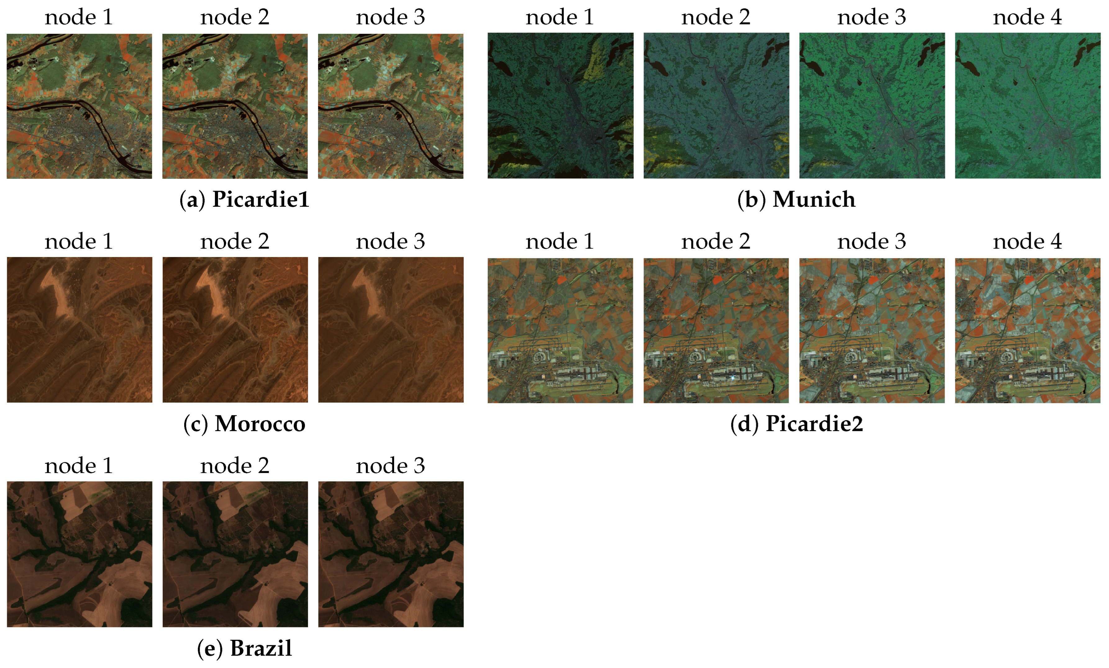
The details of the simulated datasets are provided in

Table 2. Detailed information of the simulated datasets.

Dataset	Size	Bands	Temporal	GSD (m)	Sensor
Picardie1	500 × 500	6	3	20	Sentinel-2
Picardie2	500 × 500	6	4	20	Sentinel-2
Munich	512 × 512	3	4	30	Landsat-8
Morocco	$400\times 400$	4	3	10	Sentinel-2
Brazil	$400\times 400$	4	3	10	Sentinel-2

, while representative visual examples are illustrated in Figure 1. The spatial resolution is described using ground sampling distance (GSD). Specifically, the Munich dataset is acquired from Landsat-8 with a GSD of 30 m; the Picardie1 and Picardie2 datasets are captured by Sentinel-2 with a GSD of 20 m; and the Morocco and Brazil datasets are obtained from Sentinel-2 with a GSD of 10 m. Figure 2 displays the cloud masks used in the experiments, which are extracted from real-world cloud-contaminated remote sensing images https://dataspace.copernicus.eu/ (accessed on 25 August 2025).

To quantitatively assess the cloud removal performance, we employ three widely used metrics: $\mathrm{PSNR}\left(t\right)$, $\mathrm{SSIM}\left(t\right)$, and $\mathrm{CC}\left(t\right)$, which represent the Peak Signal-to-Noise Ratio (PSNR), the Structural Similarity Index Measure (SSIM), and Correlation Coefficient (CC) at time node t, respectively. Better reconstruction performance is indicated by higher $\mathrm{PSNR}\left(t\right)$, $\mathrm{SSIM}\left(t\right)$, and $\mathrm{CC}\left(t\right)$ values. These metrics are defined as follows:

$$\mathrm{PSNR}\left(t\right)={\displaystyle \frac{1}{B}}\sum _{b=1}^{B}10\times {log}_{10}{\displaystyle \frac{{\left({\mathcal{T}}_b^t\right)}_{max}^2}{{∥{\mathcal{R}}_b^t-{\mathcal{T}}_b^t∥}_F^2}},$$

$$\mathrm{SSIM}\left(t\right)={\displaystyle \frac{1}{B}}\sum _{b=1}^B{\displaystyle \frac{\left(2{\mu }_{{\mathcal{R}}_b^t}{\mu }_{{\mathcal{T}}_b^t}+c_1\right)\left(2{\sigma }_{{\mathcal{R}}_b^t{\mathcal{T}}_b^t}+c_2\right)}{\left({\mu }_{{\mathcal{R}}_b^t}^2+{\mu }_{{\mathcal{T}}_b^t}^2+c_1\right)\left({\sigma }_{{\mathcal{R}}_b^t}^2+{\sigma }_{{\mathcal{T}}_b^t}^2+c_2\right)}},$$

$$\mathrm{CC}\left(t\right)={\displaystyle \frac{{\sum }_{i=1}^{MNB}({\mathcal{B}}_i^t-{\mu }_{\mathcal{B}})({\widehat{\mathcal{B}}}_i^t-{\mu }_{\widehat{\mathcal{B}}})}{\sqrt{{\sum }_{i=1}^{MNB}{({\mathcal{B}}_i^t-{\mu }_{\mathcal{B}})}^2{\sum }_{i=1}^{MNB}{({\widehat{\mathcal{B}}}_i^t-{\mu }_{\widehat{\mathcal{B}}})}^2}}},$$

(19)

where ${\mathcal{T}}_b^t$ denotes the b-th band of the ground truth image at time node t, and ${\mathcal{R}}_b^t$ is the corresponding reconstructed image; ${\left({\mathcal{T}}_b^t\right)}_{\max }$ is the maximum pixel value of ${\mathcal{T}}_b^t$; ${\mu }_{{\mathcal{R}}_b^t}$ and ${\sigma }_{{\mathcal{R}}_b^t}$ represent the mean and standard deviation of ${\mathcal{R}}_b^t$, respectively; ${\sigma }_{{\mathcal{R}}_b^t{\mathcal{T}}_b^t}$ denotes the covariance between ${\mathcal{R}}_b^t$ and ${\mathcal{T}}_b^t$; and $c_1$, $c_2$ are predefined constants; ${\mathcal{B}}_i^t$ and ${\widehat{\mathcal{B}}}_i^t$ denote the i-th pixel of the reconstructed and ground truth images at the t-th temporal instance, respectively. ${\mu }_{\mathcal{B}}$ and ${\mu }_{\widehat{\mathcal{B}}}$ represent their corresponding mean values.

For datasets where multiple time nodes are affected by clouds, we use the mean values of $\mathrm{PSNR}\left(t\right)$ and $\mathrm{SSIM}\left(t\right)$ across all cloud-contaminated time nodes to assess the overall cloud removal performance. These are denoted as MPSNR and MSSIM, respectively, and defined as

$$\mathrm{MPSNR}={\displaystyle \frac{1}{T^{\prime }}}\sum _{t=1}^{T^{\prime }}\mathrm{PSNR}\left(t\right),\mathrm{MSSIM}={\displaystyle \frac{1}{T^{\prime }}}\sum _{t=1}^{T^{\prime }}\mathrm{SSIM}\left(t\right)$$

(20)

where $T^{\prime }$ indicates the count of cloud-contaminated time nodes in the dataset.

4.1.2. Quantitative Comparison

The quantitative results (PSNR, SSIM, and CC) for various cloud removal techniques applied to simulated datasets are presented in

Table 3. Quantitative comparison of cloud removal approaches on synthetic datasets in terms of PSNR, SSIM, CC, and runtime. The highest results are emphasized in bold.

Dataset	Metric	Observed	HaLRTC	ALM-IPG	TVLRSDC	BC-SLRpGS	MT	Proposed
Brazil	$\mathrm{PSNR}\left(1\right)$	9.56	35.19	43.28	33.18	45.87	34.06	47.52
	$\mathrm{SSIM}\left(1\right)$	0.7436	0.9557	0.9928	0.9728	0.9937	0.8420	0.9937
	$\mathrm{CC}\left(1\right)$	0.4128	0.9941	0.9991	0.9929	0.9996	0.9916	0.9997
	Time (s)	—	7.58	79.80	57.45	311.86	219.84	72.51
Morocco	$\mathrm{PSNR}\left(1\right)$	10.50	40.96	51.23	42.87	50.96	50.96	52.84
	$\mathrm{SSIM}\left(1\right)$	0.7899	0.9837	0.9973	0.9927	0.9964	0.9512	0.9975
	$\mathrm{CC}\left(1\right)$	0.3613	0.9972	0.9998	0.9984	0.9998	0.9971	0.9998
	Time (s)	—	9.03	65.90	37.22	154.37	207.48	68.17
Munich	$\mathrm{PSNR}\left(1\right)$	12.82	36.50	33.45	35.92	35.69	32.11	38.28
	$\mathrm{SSIM}\left(1\right)$	0.8966	0.9684	0.9750	0.9640	0.9721	0.8468	0.9766
	$\mathrm{CC}\left(1\right)$	0.3546	0.9838	0.9696	0.9817	0.9804	0.9556	0.9894
	Time (s)	—	11.28	82.16	19.23	252.71	277.67	24.24
Picardie1	$\mathrm{PSNR}\left(1\right)$	7.90	45.99	52.28	48.46	53.98	46.03	54.25
	$\mathrm{SSIM}\left(1\right)$	0.6997	0.9876	0.9975	0.9923	0.9975	0.9816	0.9978
	$\mathrm{CC}\left(1\right)$	0.0555	0.9781	0.9953	0.9889	0.9967	0.9805	0.9970
	$\mathrm{PSNR}\left(2\right)$	9.52	46.70	54.44	50.75	54.75	42.85	57.12
	$\mathrm{SSIM}\left(2\right)$	0.7915	0.9889	0.9983	0.9946	0.9975	0.9596	0.9985
	$\mathrm{CC}\left(2\right)$	0.0235	0.9825	0.9971	0.9937	0.9974	0.9579	0.9985
	$\mathrm{PSNR}\left(3\right)$	11.59	48.86	51.63	50.38	54.18	42.20	56.57
	$\mathrm{SSIM}\left(3\right)$	0.8667	0.9934	0.9981	0.9959	0.9985	0.9585	0.9987
	$\mathrm{CC}\left(3\right)$	0.0602	0.9900	0.9950	0.9933	0.9971	0.9544	0.9984
	$\mathrm{MPSNR}$	9.67	47.19	52.79	49.86	54.30	43.69	55.98
	$\mathrm{MSSIM}$	0.7860	0.9900	0.9980	0.9943	0.9978	0.9666	0.9983
	$\mathrm{MCC}$	0.0464	0.9835	0.9958	0.9920	0.9971	0.9643	0.9980
	Time (s)	—	40.07	109.63	69.31	495.80	990.88	78.92
Picardie2	$\mathrm{PSNR}\left(1\right)$	7.50	46.50	51.86	47.38	51.45	43.19	52.82
	$\mathrm{SSIM}\left(1\right)$	0.7306	0.9914	0.9976	0.9932	0.9972	0.9694	0.9971
	$\mathrm{CC}\left(1\right)$	0.0765	0.9709	0.9921	0.9787	0.9912	0.9385	0.9934
	$\mathrm{PSNR}\left(2\right)$	7.90	47.41	44.39	43.03	44.22	43.29	51.40
	$\mathrm{SSIM}\left(2\right)$	0.6992	0.9918	0.9979	0.9921	0.9961	0.9695	0.9968
	$\mathrm{CC}\left(2\right)$	0.0004	0.9811	0.9624	0.9521	0.9622	0.9528	0.9929
	$\mathrm{PSNR}\left(3\right)$	9.67	48.22	55.76	50.31	54.85	41.92	55.02
	$\mathrm{SSIM}\left(3\right)$	0.7937	0.9932	0.9987	0.9952	0.9980	0.9631	0.9981
	$\mathrm{CC}\left(3\right)$	0.0653	0.9852	0.9974	0.9908	0.9969	0.9383	0.9970
	$\mathrm{PSNR}\left(4\right)$	11.73	48.36	54.53	50.35	53.63	42.20	55.75
	$\mathrm{SSIM}\left(4\right)$	0.8681	0.9950	0.9988	0.9963	0.9984	0.9599	0.9985
	$\mathrm{CC}\left(4\right)$	0.1084	0.9876	0.9970	0.9922	0.9964	0.9480	0.9978
	$\mathrm{MPSNR}$	9.20	47.62	51.63	47.77	51.04	42.65	53.75
	$\mathrm{MSSIM}$	0.7729	0.9929	0.9982	0.9942	0.9974	0.9655	0.9976
	$\mathrm{MCC}$	0.0627	0.9812	0.9872	0.9785	0.9867	0.9444	0.9953
	Time (s)	—	26.48	151.78	231.91	235.20	1220.11	152.48
Average for All Data	PSNR	9.87	44.47	49.29	45.26	49.96	41.88	52.16
	SSIM	0.7880	0.9849	0.9952	0.9889	0.9945	0.9402	0.9953
	CC	0.2476	0.9880	0.9903	0.9887	0.9927	0.9706	0.9964
	Time (s)	—	18.89	97.85	83.02	289.99	583.20	79.26

, with the highest values for each metric highlighted in bold. In this table, $\mathrm{PSNR}\left(t\right)$, $\mathrm{SSIM}\left(t\right)$, and $\mathrm{CC}\left(t\right)$ represent the PSNR, SSIM, and CC values at time node t, while MPSNR, MSSIM, and MCC denote the average PSNR, SSIM, and CC across all cloud-contaminated time nodes.

To better reflect the complexity of cloud distributions in real-world remote sensing scenarios, the test datasets include Brazil, Morocco, and Munich, where only the first time node is contaminated by clouds, as well as Picardie1 and Picardie2, which contain clouds in multiple time nodes.

As shown in the table, the proposed method outperforms the others in terms of PSNR, SSIM, and CC in most cases. For the Picardie2 dataset, all the temporal images are cloud-contaminated, with certain spatial regions occluded in every time node, making reconstruction particularly challenging. As reported in Table 3, the proposed method achieves the highest MPSNR, MSSIM, and MCC, demonstrating strong robustness under severe degradation. At time node 2, the relative improvement compared with the other time nodes is smaller, which may be due to higher scene complexity and more pronounced land-cover variation, but the proposed method still delivers superior PSNR, SSIM, and CC compared with all the competing approaches. Moreover, across all four time nodes, the proposed method maintains relatively stable numerical performance in contrast to some competing methods, where accuracy varies substantially between time nodes.

In conclusion, the proposed method achieves the highest average performance across all the datasets, with an average PSNR of 52.16 dB and SSIM of 0.9953, clearly outperforming all the competing methods. In addition to accuracy, Table 3 also reports the runtime (in seconds) of each method on the same hardware platform. The proposed method attains comparable efficiency to model-based methods such as TVLRSDC and ALM-IPG while being substantially faster than deep learning approaches that involve large-scale network inference. This demonstrates that our method strikes a favorable balance between reconstruction quality and computational efficiency. These results highlight the effectiveness and practicality of the proposed continuous blind cloud removal framework under diverse cloud conditions.

4.1.3. Qualitative Comparison

In this section, we compare the cloud removal capabilities of different methods by presenting both the visual results and the residual maps (i.e., residual between the reconstruction and the ground truth).

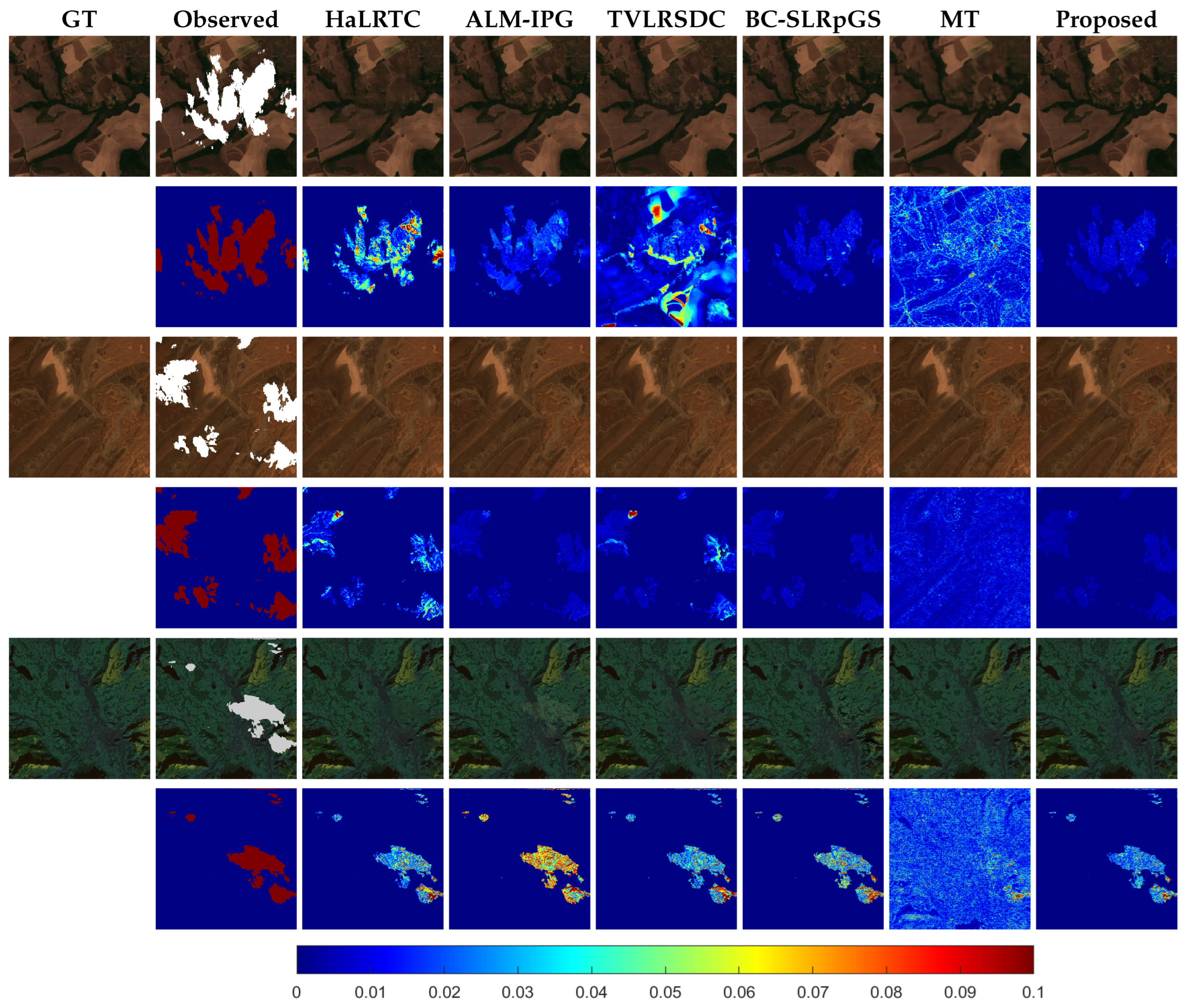
The results for the Brazil, Morocco, and Munich datasets are illustrated in Figure 3, arranged from top to bottom in the corresponding order. For each dataset, the top row showcases the cloud removal results, while the corresponding residual maps are shown below. In these simulated experiments, only the first time node is contaminated by clouds. As shown in the figure, all the methods produce visually promising reconstructions. However, the residual maps reveal more detailed differences. Specifically, the HaLRTC, ALM-IPG, TVLRSDC, and BC-SLRpGS methods exhibit large residuals compared to the ground truth, as indicated by the presence of red regions in their residual maps. Although the MT method does not produce large red areas in the residual maps, it changes the information in regions that were not contaminated by clouds in the observed image, resulting in lower overall reconstruction quality. Conversely, the proposed method not only achieves superior visual quality but also yields the smallest residuals, with the least presence of red regions in the residual maps. This implies that our method produces reconstructed images that are nearest to the ground truth when compared to all the others.

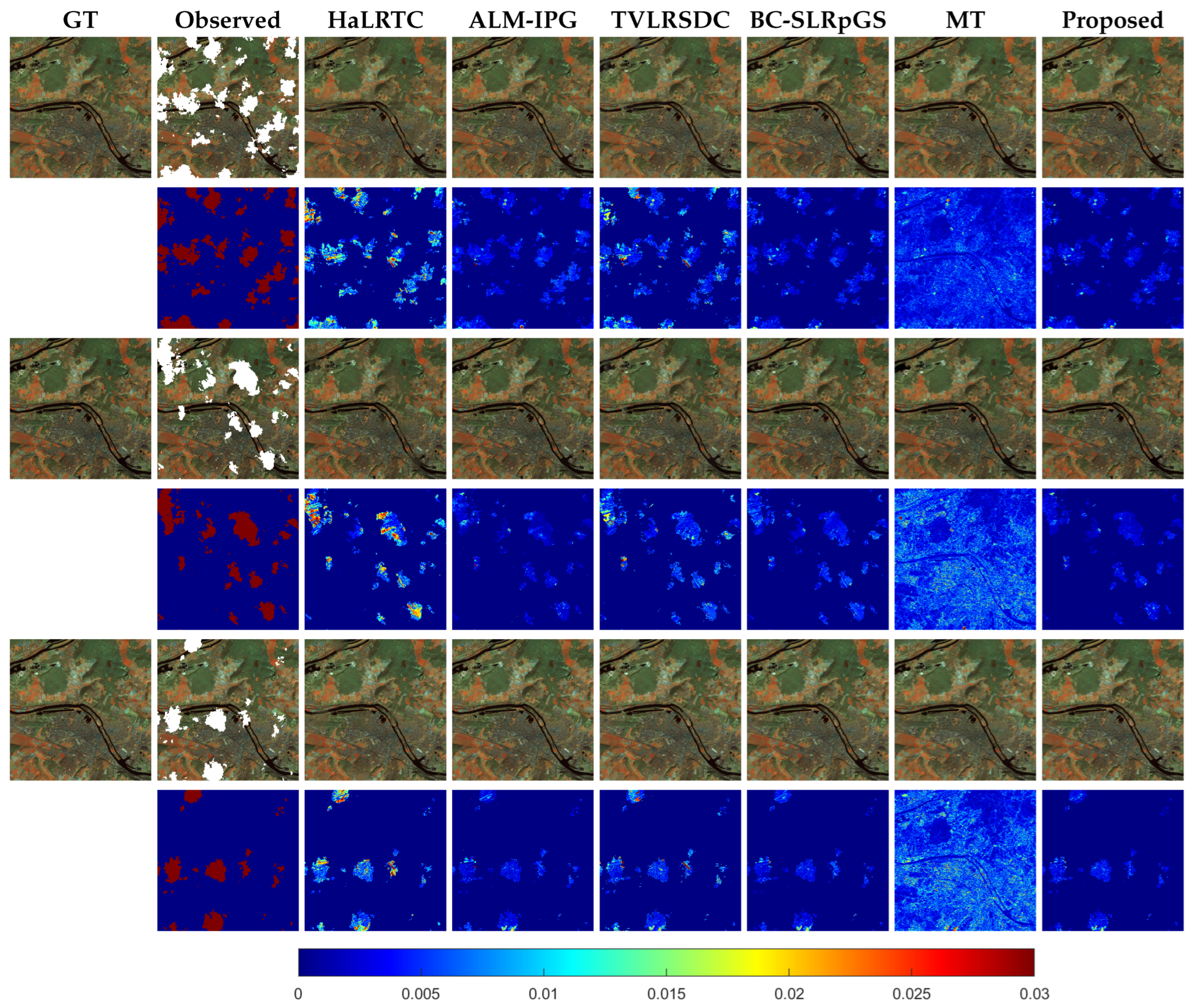
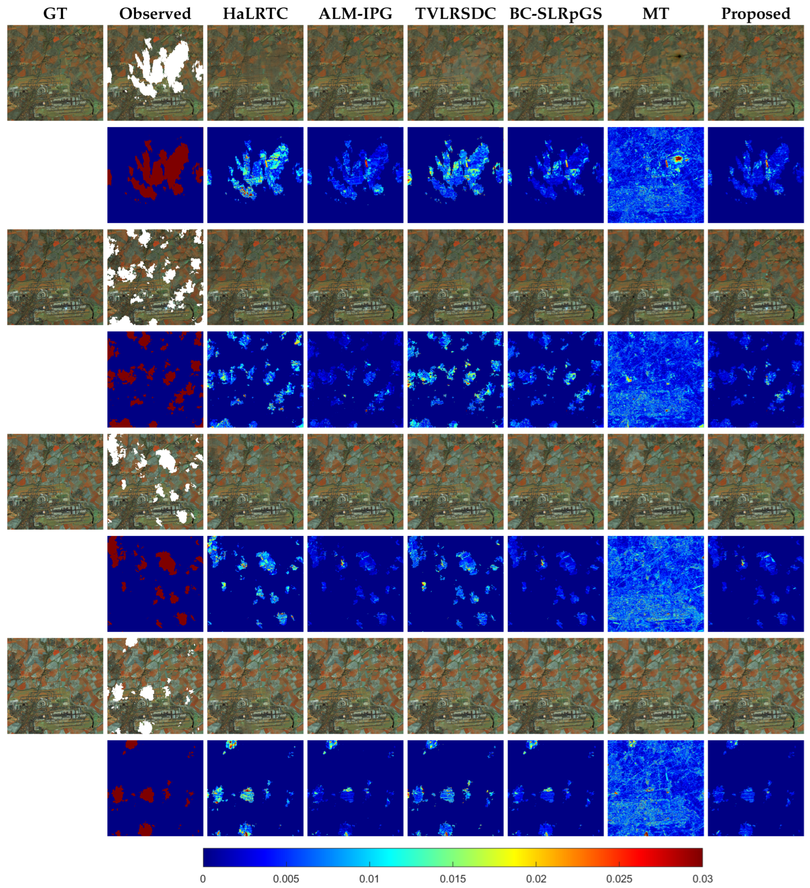
The results of cloud removal for each method on the Picardie1 and Picardie2 datasets are presented in Figure 4 and Figure 5, respectively. In both datasets, all the temporal images are cloud-contaminated, and some spatial regions are occluded across all the time nodes. This leads to severe information loss and poses significant challenges for cloud removal. From the figures, it can be observed that the performance of cloud removal by HaLRTC, TVLRSDC, and MT is less satisfactory. For example, HaLRTC produces overly smooth results and loses substantial detail; TVLRSDC shows inconsistencies between the reconstructed regions and their surroundings; and MT changes the information in regions that were not contaminated by clouds in the observed image, leading to degraded visual quality. In contrast, ALM-IPG, BC-SLRpGS, and our approach yield more accurate and visually consistent reconstructions. Among them, a cloud mask for ALM-IPG is provided, while BC-SLRpGS and our approach perform blind cloud removal. The residual maps further demonstrate that the proposed method results in fewer large residual values, indicating that it preserves more fine details and achieves reconstructions closer to the ground truth.

4.2. Real Experiments

In this part, we assess the cloud removal effectiveness of the approach presented on two real-world cloud-contaminated datasets.

4.2.1. Data

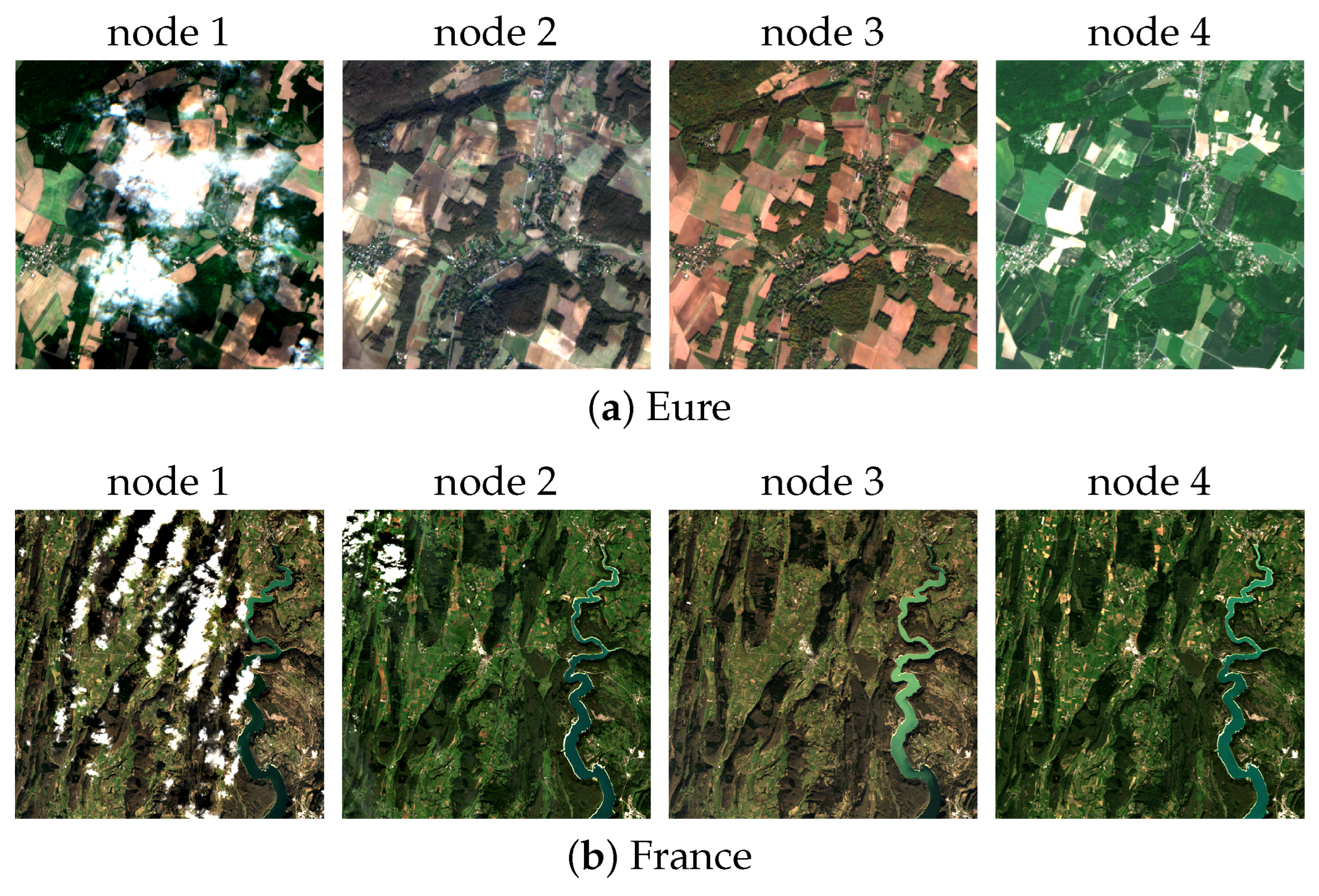
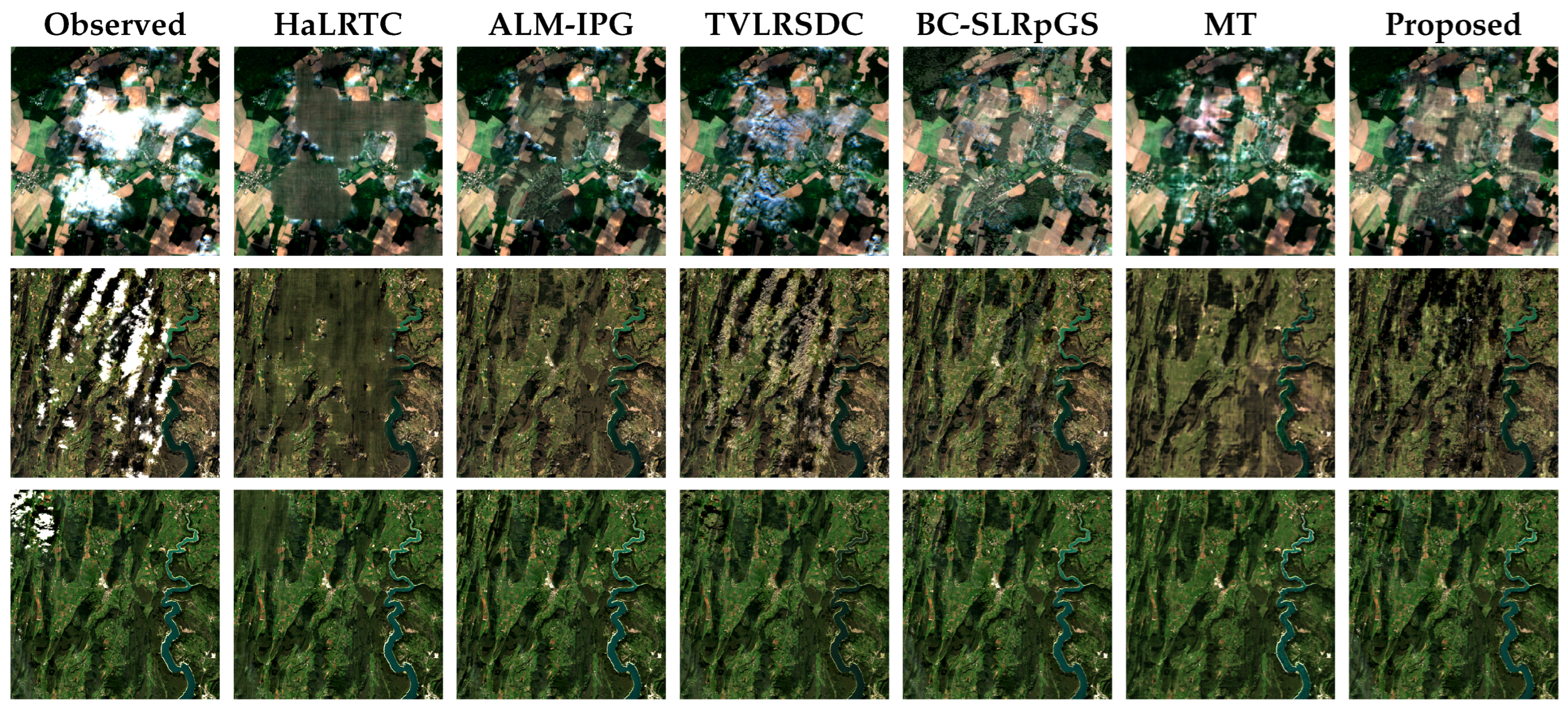
The detailed information of the real datasets used in this section is summarized in

Table 4. Detailed information of the real-world datasets.

Dataset	Size	Bands	Temporal	GSD (m)	Sensor
Eure	400 × 400	4	4	10	Sentinel-2
France	600 × 600	7	4	30	Landsat-8

, and the corresponding visual examples are provided in Figure 6. The Eure dataset, captured by Sentinel-2 with a spatial resolution of 10 meters, consists of four time nodes (each with four spectral bands), one of which is contaminated by clouds. The France dataset, acquired by Landsat-8 with a spatial resolution of 30 meters, also contains four time nodes (each with seven bands), two of which are cloud-contaminated. Figure 6 shows that images captured at different times in both datasets exhibit significant variations, further increasing the difficulty of cloud removal.

4.2.2. Qualitative Comparison

The cloud removal outcomes for all the methods across the two real-world datasets are shown in Figure 7. The results for the Eure dataset are presented in the first row, while the second and third rows provide the outcomes for the first and second cloud-contaminated time nodes of the France dataset. As shown in the figure, HaLRTC fails to effectively reconstruct the cloud-covered areas, particularly on the Eure dataset, where it is unable to recover any meaningful information. The results from ALM-IPG exhibit noticeable differences in comparison to the reconstructed parts and the surrounding areas free from clouds. The results of TVLRSDC and MT still contain visible cloud information, suggesting that they fail to fully restore the cloud-contaminated information. Both BC-SLRpGS and the proposed method achieve visually pleasing results. Significantly, the proposed method better preserves details, demonstrating its superior ability to recover structural information in real-world cloud-contaminated remote sensing images.

4.2.3. Cloud Detection Results

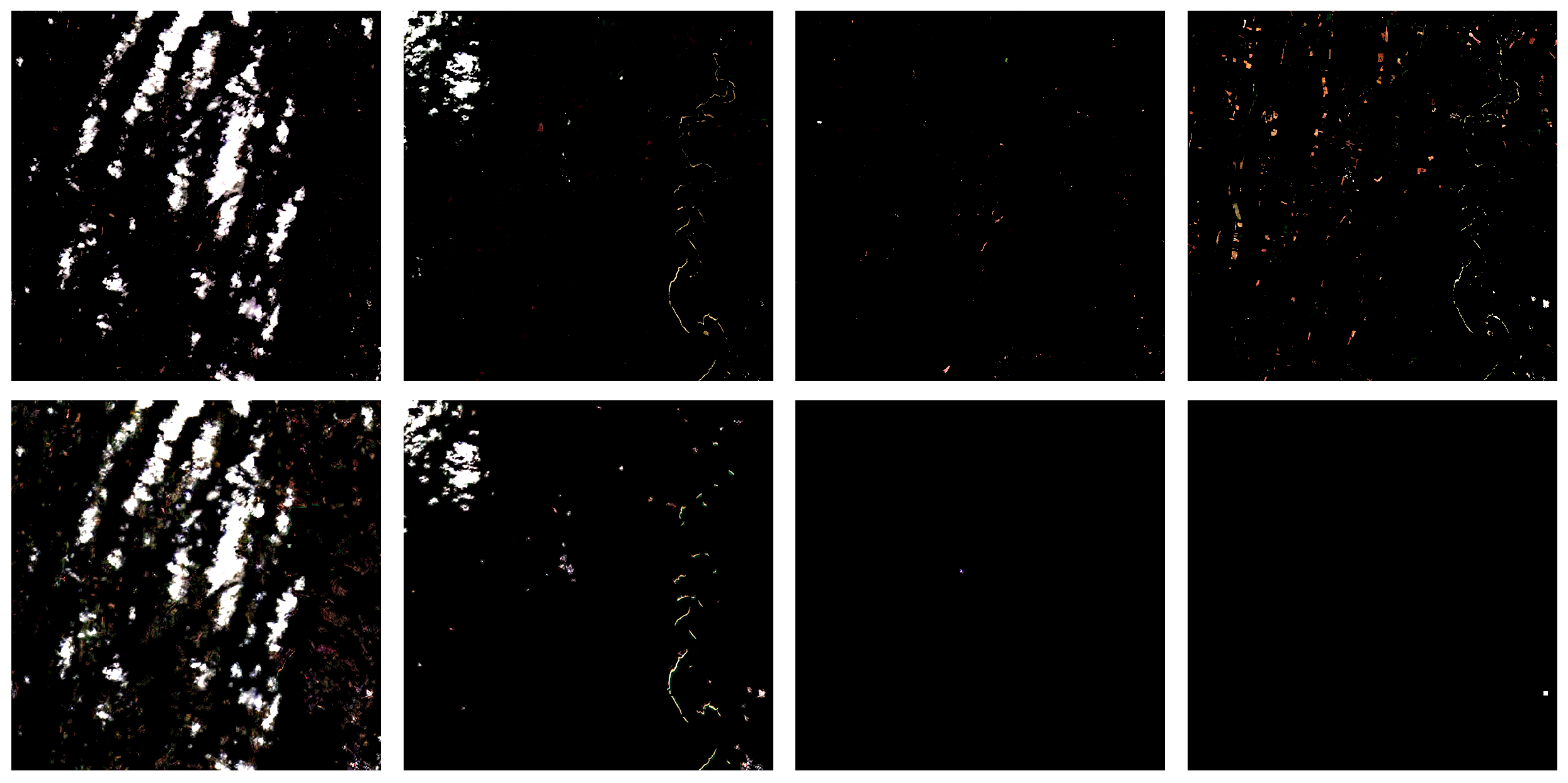
In this section, we evaluate the cloud detection performance of the proposed method. Among the comparison methods, TVLRSDC, BC-SLRpGS, MT, and our approach are all blind cloud removal approaches. As demonstrated in previous experiments, both TVLRSDC and MT tend to change information in areas unaffected by clouds in the observed image, indicating poor cloud detection performance. Therefore, our analysis in this section focuses on comparing the cloud detection performance of BC-SLRpGS and our approach.

The results of cloud detection (i.e., the estimated cloud components) on both the Eure and France datasets are illustrated in Figure 8 and Figure 9. In each figure, the first row shows the cloud detection results of BC-SLRpGS, while the second row illustrates the outcomes of our approach. From the figures, we observe that, for time nodes without cloud contamination (e.g., the second, third, and fourth time nodes of the Eure dataset, and the third and fourth time nodes of the France dataset), BC-SLRpGS incorrectly identifies non-cloud regions as clouds. This misdetection leads to undesired modifications in the clean temporal images, ultimately degrading the overall reconstruction quality. In contrast, the proposed method detects almost no cloud components in these cloud-free time node images, demonstrating its ability to preserve the original content where no cloud is present. These results demonstrate that, compared with BC-SLRpGS, the proposed method achieves more precise cloud detection, which in turn contributes to more effective and reliable cloud removal.

4.3. Scalability on Large-Size Images

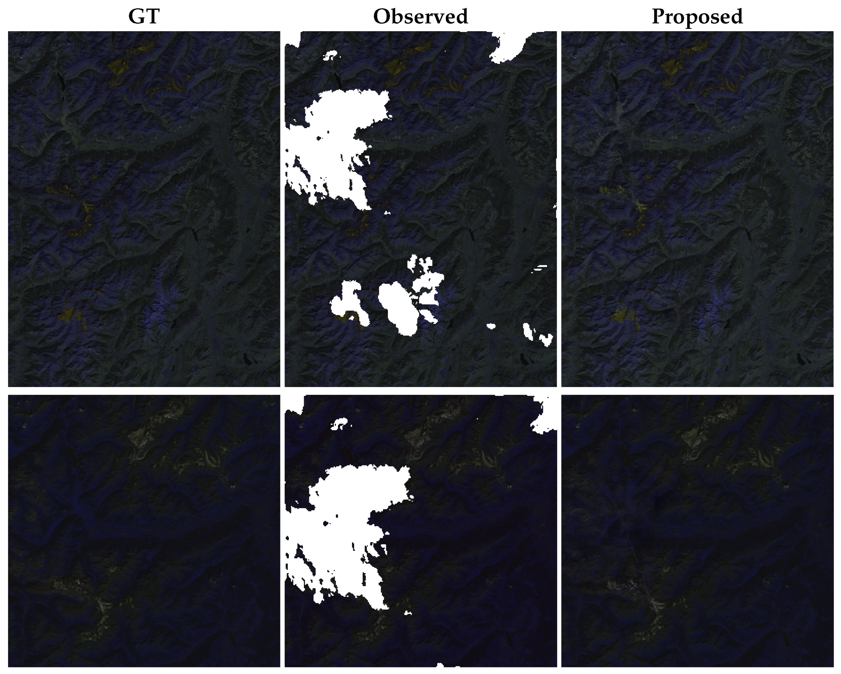
To further evaluate the scalability of the proposed method, we performed experiments on large remote sensing images with sizes of $4200\times 5490$ and $7000\times 7000$ pixels https://dataspace.copernicus.eu/data-collections (accessed on 25 August 2025). As reported in

Table 5. Quantitative performance of the proposed method on large-size remote sensing images.

Dataset	Size (k × k)	PSNR (dB)	SSIM	Time (min)
Large-1	$4200\times 5490$	41.29	0.9842	21.25
Large-2	$7000\times 7000$	42.75	0.9905	33.53

, the method consistently achieves high reconstruction accuracy (PSNR above 41 dB and SSIM over 0.98) while maintaining practical computational efficiency (20–34 min per image).

All large-scale experiments were conducted on a server equipped with an Intel Xeon(R) Gold 6348 CPU (2.60GHz, Intel Corporation, Santa Clara, CA, USA) with 100GB RAM and an NVIDIA A800 (80 GB memory, NVIDIA Corporation, Santa Clara, CA, USA). The method was implemented in PyTorch 2.1.2 with CUDA 11.8, and the runtime reported in Table 5 corresponds to single-GPU execution.

Figure 10 provides visual examples on the two large test images, showing that the proposed approach successfully reconstructs fine spatial structures even at very high resolutions. These results confirm that the continuous tensor function representation scales well and is applicable to large-scale remote sensing scenarios in practice.

4.4. Ablation Study

To evaluate the contribution of the continuous tensor function representation, we replaced it with a discrete low-rank Tucker decomposition while keeping all the other settings unchanged. As shown in

Table 6. Ablation: continuous vs. discrete low-rank representation on the Munich dataset.

Method	PSNR (dB)	SSIM
Discrete low-rank Tucker	37.35	0.9719
Continuous tensor function (Ours)	38.28	0.9766

, our continuous formulation achieves notable improvements, demonstrating its superior capability in modeling fine image details.

To evaluate the influence of the temporal dimension T on the performance of the proposed method, we conducted experiments on the Munich simulated dataset with $T\in \{1,2,3,4\}$.

Table 7. Effect of temporal dimension T on the performance of the proposed method on the Munich dataset.

T	PSNR (dB)	SSIM
1	33.38	0.9455
2	37.38	0.9720
3	37.96	0.9758
4	38.28	0.9766

reports the quantitative results in terms of PSNR and SSIM. It can be observed that increasing T consistently improves the restoration quality. For example, the PSNR increases from 33.38 dB at $T=1$ to 38.28 dB at $T=4$, and the SSIM improves from 0.9455 to 0.9766. This performance gain can be attributed to the richer complementary information and temporal redundancy provided by additional cloud-free observations, which facilitate more accurate recovery of cloud-covered regions.

In addition, we clarify that the morphological erosion step is adopted as a preprocessing operation to stabilize the detection with different quantile levels. Without erosion, a smaller quantile threshold $q_t$ is typically required to achieve accurate detection, whereas, with erosion, comparable detection results can be obtained even with a larger quantile threshold $q_t^{\prime }>q_t$, where $q_t$ and $q_t^{\prime }$ denote the quantile levels before and after applying morphological erosion, respectively. Since morphological erosion is not the main contribution of this work, we keep it as a fixed auxiliary operation rather than a tunable component and do not provide further ablation studies on this factor.

4.5. Hyperparameter Sensitivity Analysis

We further conducted a sensitivity analysis on three key hyperparameters of the proposed method: the quantile level $q_t$ in cloud detection, and the regularization parameters ${\lambda }_1$ and ${\lambda }_2$. Experiments were performed on the Munich dataset, and the PSNR values were recorded while varying each parameter independently. Specifically, $q_t$ is varied from 0.0 to 1.0 with a step size of 0.1, while ${\lambda }_1$ and ${\lambda }_2$ are tested with values $\{{10}^{-7},{10}^{-6},{10}^{-5},{10}^{-4},{10}^{-3},{10}^{-2},{10}^{-1},{10}^0\}$.

The results are plotted in Figure 11. As shown, when $q_t$ increases, PSNR initially rises and reaches its maximum at $q_t=0.9$, then decreases. This is because a smaller $q_t$ corresponds to a lower threshold, leading to larger detected cloud regions and potentially more false positives. For ${\lambda }_1$ and ${\lambda }_2$, PSNR remains relatively stable with minor fluctuations for the first seven values but decreases when either parameter reaches ${10}^0$, indicating that excessively large regularization weights may over-smooth the reconstruction. These results suggest that $q_t$ values around 0.9 and ${\lambda }_1,{\lambda }_2\in [{10}^{-7},{10}^{-1}]$ offer robust performance.

5. Conclusions

This paper proposed a novel continuous blind cloud removal model to address the limitations of the existing discrete low-rank and sparse prior-based methods. Unlike traditional approaches that rely on manually designed regularization terms, the proposed method represents the cloud-free image component using a continuous tensor function that integrates implicit neural representations with low-rank tensor decomposition. This formulation enables more accurate modeling of both global correlations and local smoothness in remote sensing imagery. In the case of the cloud component, we implemented a band-wise sparse function that effectively captures both the spectral and spatial features of clouds. To retain the details in cloud-free regions while reconstructing, we designed a box constraint guided by an adaptive thresholding-based cloud detection strategy, further enhanced by morphological erosion to ensure precise delineation of cloud boundaries. An alternating minimization algorithm was designed to effectively address the proposed model. Extensive evaluations on both simulated and real-world datasets showed that our method consistently outperforms or remains competitive with state-of-the-art approaches in terms of both visual quality and quantitative metrics. These results validate the efficiency and reliability of the proposed continuous framework in tackling the cloud removal challenges in optical remote sensing imagery.

While the proposed method demonstrates strong performance across diverse datasets, several limitations remain. First, when applied to extremely large-scale datasets or ultra-high-resolution images, the computational cost may become significant due to the optimization-based nature of the approach, even though our experiments show competitive runtime on moderate-scale data. Second, in scenes with highly dynamic land-cover changes (e.g., rapid vegetation growth or seasonal flooding), the temporal smoothness prior in our model may not fully capture abrupt variations, potentially leading to over-smoothing or incomplete reconstruction in rapidly changing regions.

In future work, we will focus on improving the scalability of the method for large-scale datasets, enhancing adaptability to highly dynamic scenes, and exploring the integration of multimodal data to further improve reconstruction performance.

References

1. Wang, Z.; Chen, T.; Zhu, D.; Jia, K.; Plaza, A. Rseife: A new remote sensing ecological index for simulating the land surface eco-environment. J. Environ. Manag. 2023, 326, 116851. [Google Scholar] [CrossRef]
2. Maity, S.; Das, S.; Pattanayak, J.M.; Bera, B.; Shit, P.K. Assessment of ecological environment quality in kolkata urban agglomeration, india. Urban Ecosyst. 2022, 25, 1137–1154. [Google Scholar] [CrossRef]
3. Sharma, S.; Beslity, J.O.; Rustad, L.; Shelby, L.J.; Manos, P.T.; Khanal, P.; Reinmann, A.B.; Khanal, C. Remote Sensing and GIS in Natural Resource Management: Comparing Tools and Emphasizing the Importance of In-Situ Data. Remote Sens. 2024, 16, 4161. [Google Scholar] [CrossRef]
4. Wei, R.; Feng, Z.; Wu, Z.; Yu, C.; Song, B.; Cao, C. Optical remote sensing image target detection based on improved feature pyramid. IEEE J. Sel. Top. Appl. Earth Obs. Remote Sens. 2023, 16, 7507–7517. [Google Scholar] [CrossRef]
5. Wang, Y. Research on remote sensing image target detection algorithm based on optical measurement information. In Proceedings of the 2022 IEEE Conference on Telecommunications, Optics and Computer Science (TOCS), Online, 11–12 December 2022; pp. 1243–1248. [Google Scholar]
6. Chen, Y.; Lai, W.; He, W.; Zhao, X.L.; Zeng, J. Hyperspectral Compressive Snapshot Reconstruction via Coupled Low-Rank Subspace Representation and Self-Supervised Deep Network. IEEE Trans. Image Process. 2024, 33, 926–941. [Google Scholar] [CrossRef]
7. Ju, J.; Roy, D.P. The availability of cloud-free landsat ETM+ data over the conterminous united states and globally. Remote Sens. Environ. 2008, 112, 1196–1211. [Google Scholar] [CrossRef]
8. Chen, T.; Lv, L.; Wang, D.; Zhang, J.; Yang, Y.; Zhao, Z.; Wang, C.; Guo, X.; Chen, H.; Wang, Q.; et al. Empowering Agrifood System With Artificial Intelligence: A Survey of The Progress, Challenges and Opportunities. ACM Comput. Surv. 2025, 57, 1–37. [Google Scholar] [CrossRef]
9. He, K.; Sun, J. Image Completion Approaches Using the Statistics of Similar Patches. IEEE Trans. Pattern Anal. Mach. Intell. 2014, 36, 2423–2435. [Google Scholar] [CrossRef] [PubMed]
10. Cheng, Q.; Shen, H.; Zhang, L.; Li, P. Inpainting for Remotely Sensed Images With a Multichannel Nonlocal Total Variation Model. IEEE Trans. Geosci. Remote Sens. 2014, 52, 175–187. [Google Scholar] [CrossRef]
11. Bertalmio, M.; Vese, L.; Sapiro, G.; Osher, S. Simultaneous structure and texture image inpainting. IEEE Trans. Image Process. 2003, 12, 882–889. [Google Scholar] [CrossRef] [PubMed]
12. Zhu, X.; Gao, F.; Liu, D.; Chen, J. A Modified Neighborhood Similar Pixel Interpolator Approach for Removing Thick Clouds in Landsat Images. IEEE Geosci. Remote Sens. Lett. 2012, 9, 521–525. [Google Scholar] [CrossRef]
13. Maalouf, A.; Carre, P.; Augereau, B.; Fernandez-Maloigne, C. A Bandelet-Based Inpainting Technique for Clouds Removal From Remotely Sensed Images. IEEE Trans. Geosci. Remote Sens. 2009, 47, 2363–2371. [Google Scholar] [CrossRef]
14. Shen, H.; Li, X.; Zhang, L.; Tao, D.; Zeng, C. Compressed Sensing-Based Inpainting of Aqua Moderate Resolution Imaging Spectroradiometer Band 6 Using Adaptive Spectrum-Weighted Sparse Bayesian Dictionary Learning. IEEE Trans. Geosci. Remote Sens. 2014, 52, 894–906. [Google Scholar] [CrossRef]
15. Li, X.; Shen, H.; Zhang, L.; Zhang, H.; Yuan, Q. Dead Pixel Completion of Aqua MODIS Band 6 Using a Robust M-Estimator Multiregression. IEEE Geosci. Remote Sens. Lett. 2014, 11, 768–772. [Google Scholar]
16. Shen, H.; Zeng, C.; Zhang, L. Recovering Reflectance of AQUA MODIS Band 6 Based on Within-Class Local Fitting. IEEE J. Sel. Top. Appl. Earth Obs. Remote Sens. 2011, 4, 185–192. [Google Scholar] [CrossRef]
17. Yang, S.J.; Zheng, Y.B.; Li, H.C.; Chen, Y.; Zhu, Q. Spectral-Temporal Consistency Prior for Cloud Removal From Remote Sensing Images. IEEE Trans. Geosci. Remote Sens. 2025, 63, 5400212. [Google Scholar] [CrossRef]
18. Lin, C.H.; Tsai, P.H.; Lai, K.H.; Chen, J.Y. Cloud removal from multitemporal satellite images using information cloning. IEEE Trans. Geosci. Remote Sens. 2012, 51, 232–241. [Google Scholar] [CrossRef]
19. Li, Z.; Shen, H.; Cheng, Q.; Li, W.; Zhang, L. Thick cloud removal in high-resolution satellite images using stepwise radiometric adjustment and residual correction. Remote Sens. 2019, 11, 1925. [Google Scholar] [CrossRef]
20. Peng, H.; Huang, T.Z.; Zhao, X.L.; Lin, J.; Wu, W.H.; Li, L.Y. Deep Domain Fidelity and Low-Rank Tensor Ring Regularization for Thick Cloud Removal of Multitemporal Remote Sensing Images. IEEE Trans. Geosci. Remote Sens. 2024, 62, 5409314. [Google Scholar] [CrossRef]
21. Li, L.Y.; Huang, T.Z.; Zheng, Y.B.; Zheng, W.J.; Wu, G.C.; Zhao, X.L. Thick Cloud Removal for Multitemporal Remote Sensing Images: When Tensor Ring Decomposition Meets Gradient Domain Fidelity. IEEE Trans. Geosci. Remote Sens. 2023, 61, 5512414. [Google Scholar] [CrossRef]
22. Shen, H.; Wu, J.; Cheng, Q.; Aihemaiti, M.; Zhang, C.; Li, Z. A spatiotemporal fusion based cloud removal method for remote sensing images with land cover changes. IEEE J. Sel. Top. Appl. Earth Obs. Remote Sens. 2019, 12, 862–874. [Google Scholar] [CrossRef]
23. Chen, J.; Jönsson, P.; Tamura, M.; Gu, Z.; Matsushita, B.; Eklundh, L. A Simple Method for Reconstructing a High-Quality NDVI Time-Series Data Set Based on The Savitzky-Golay Filter. Remote Sens. Environ. 2004, 91, 332–344. [Google Scholar] [CrossRef]
24. Chen, B.; Huang, B.; Chen, L.; Xu, B. Spatially and Temporally Weighted Regression: A Novel Method to Produce Continuous Cloud-Free Landsat Imagery. IEEE Trans. Geosci. Remote Sens. 2017, 55, 27–37. [Google Scholar] [CrossRef]
25. Liu, J.; Musialski, P.; Wonka, P.; Ye, J. Tensor completion for estimating missing values in visual data. IEEE Trans. Pattern Anal. Mach. Intell. 2013, 35, 208–220. [Google Scholar] [CrossRef]
26. Wang, J.; Olsen, P.A.; Conn, A.R.; Lozano, A.C. Removing clouds and recovering ground observations in satellite image sequences via temporally contiguous robust matrix completion. In Proceedings of the IEEE Conference on Computer Vision and Pattern Recognition, Las Vegas, NV, USA, 27–30 June 2016; pp. 2754–2763. [Google Scholar]
27. Chen, Y.; He, W.; Yokoya, N.; Huang, T.Z. Blind cloud and cloud shadow removal of multitemporal images based on total variation regularized low-rank sparsity decomposition. ISPRS J. Photogramm. Remote Sens. 2019, 157, 93–107. [Google Scholar] [CrossRef]
28. Ji, T.Y.; Chu, D.; Zhao, X.L.; Hong, D. A Unified Framework of Cloud Detection and Removal Based on Low-Rank and Group Sparse Regularizations for Multitemporal Multispectral Images. IEEE Trans. Geosci. Remote Sens. 2022, 60, 5303015. [Google Scholar] [CrossRef]
29. Wang, L.; Wang, Q.; Tong, X.; Atkinson, P.M. MST-Net: A General Deep Learning Model for Thick Cloud Removal From Optical Images. IEEE Trans. Geosci. Remote Sens. 2025, 63, 5612518. [Google Scholar] [CrossRef]
30. Chen, Y.; Weng, Q.; Tang, L.; Zhang, X.; Bilal, M.; Li, Q. Thick Clouds Removing From Multitemporal Landsat Images Using Spatiotemporal Neural Networks. IEEE Trans. Geosci. Remote Sens. 2022, 60, 4400214. [Google Scholar] [CrossRef]
31. Ji, S.; Dai, P.; Lu, M.; Zhang, Y. Simultaneous Cloud Detection and Removal From Bitemporal Remote Sensing Images Using Cascade Convolutional Neural Networks. IEEE Trans. Geosci. Remote Sens. 2021, 59, 732–748. [Google Scholar] [CrossRef]
32. Zhang, Q.; Yuan, Q.; Li, J.; Li, Z.; Shen, H.; Zhang, L. Thick cloud and cloud shadow removal in multitemporal imagery using progressively spatio-temporal patch group deep learning. ISPRS J. Photogramm. Remote Sens. 2020, 162, 148–160. [Google Scholar] [CrossRef]
33. Chen, Y.; Chen, M.; He, W.; Zeng, J.; Huang, M.; Zheng, Y.B. Thick Cloud Removal in Multitemporal Remote Sensing Images via Low-Rank Regularized Self-Supervised Network. IEEE Trans. Geosci. Remote Sens. 2024, 62, 5506613. [Google Scholar] [CrossRef]
34. Du, C.; Xiao, J.; Li, J.; Liu, Y.; He, J.; Yuan, Q. SSGT: Spatiospectral Guided Transformer for Hyperspectral Image Fusion Joint With Cloud Removal. IEEE J. Sel. Top. Appl. Earth Obs. Remote Sens. 2025, 18, 3472–3487. [Google Scholar] [CrossRef]
35. Wu, Y.; Deng, Y.; Zhou, S.; Liu, Y.; Huang, W.; Wang, J. CR-former: Single-Image Cloud Removal With Focused Taylor Attention. IEEE Trans. Geosci. Remote Sens. 2024, 62, 5651614. [Google Scholar] [CrossRef]
36. Rui, Q.; He, S.; Li, T.; Wang, G.; Ruan, N.; Mei, L.; Yang, Y.; Shen, H. Density-Aware Cloud Removal of Remote Sensing Imagery Using a Global-Local Fusion Transformer. IEEE Trans. Geosci. Remote Sens. 2024, 62, 5651511. [Google Scholar] [CrossRef]
37. Dou, A.; Hao, Y.; Liu, W.; Li, L.; Wang, Z.; Liu, B. Remote Sensing Image Cloud Removal Based on Multi-Scale Spatial Information Perception. Multimed. Syst. 2024, 30, 249. [Google Scholar] [CrossRef]
38. Zhou, H.; Wang, Y.; Liu, W.; Tao, D.; Ma, W.; Liu, B. MSC-GAN: A Multistream Complementary Generative Adversarial Network With Grouping Learning for Multitemporal Cloud Removal. IEEE Trans. Geosci. Remote Sens. 2025, 63, 5400117. [Google Scholar] [CrossRef]
39. Yang, J.; Wang, W.; Chen, K.; Liu, L.; Zou, Z.; Shi, Z. Structural Representation-Guided GAN for Remote Sensing Image Cloud Removal. IEEE Geosci. Remote Sens. Lett. 2025, 22, 6002105. [Google Scholar] [CrossRef]
40. Darbaghshahi, F.N.; Mohammadi, M.R.; Soryani, M. Cloud Removal in Remote Sensing Images Using Generative Adversarial Networks and SAR-to-Optical Image Translation. IEEE Trans. Geosci. Remote Sens. 2022, 60, 6002105. [Google Scholar] [CrossRef]
41. Wang, Y.; Zhang, B.; Zhang, W.; Hong, D.; Zhao, B.; Li, Z. Cloud Removal With SAR-Optical Data Fusion Using a Unified Spatial–Spectral Residual Network. IEEE Trans. Geosci. Remote Sens. 2024, 62, 5600820. [Google Scholar] [CrossRef]
42. Czerkawski, M.; Upadhyay, P.; Davison, C.; Werkmeister, A.; Cardona, J.; Atkinson, R.; Michie, C.; Andonovic, I.; Macdonald, M.; Tachtatzis, C. Deep Internal Learning for Inpainting of Cloud-Affected Regions in Satellite Imagery. Remote Sens. 2022, 14, 1342. [Google Scholar] [CrossRef]
43. Luo, Y.; Zhao, X.; Li, Z.; Ng, M.K.; Meng, D. Low-Rank Tensor Function Representation for Multi-Dimensional Data Recovery. IEEE Trans. Pattern Anal. Mach. Intell. 2024, 46, 3351–3369. [Google Scholar] [CrossRef] [PubMed]
44. Kolda, T.G.; Bader, B.W. Tensor decompositions and applications. SIAM Rev. 2009, 51, 455–500. [Google Scholar] [CrossRef]
45. Sitzmann, V.; Martel, J.; Bergman, A.; Lindell, D.; Wetzstein, G. Implicit Neural Representations with Periodic Activation Functions. In Advances in Neural Information Processing Systems; Curran Associates, Inc.: Red Hook, NY, USA, 2020; Volume 33, pp. 7462–7473. [Google Scholar]
Figure 1. Visual illustrations of the simulated datasets used in the experiments.
Remotesensing 17 03001 g001
Figure 2. Cloud masks used in the synthetic experiments.
Remotesensing 17 03001 g002
Figure 3. Cloud removal results on the simulated datasets. The results for Brazil, Morocco, and Munich datasets are presented from top to bottom. For dataset, the first row shows the visual results of cloud removal, and the second row displays the corresponding residual maps (red = high residual; blue = low residual).
Remotesensing 17 03001 g003
Figure 4. Cloud removal results on the simulated Picardie1 dataset. From top to bottom are the results at time points 1 to 3. For each time point, the first row shows the visual results of cloud removal, and the second row displays the corresponding residual maps (red = high residual; blue = low residual).
Remotesensing 17 03001 g004
Figure 5. Cloud removal results on the simulated Picardie2 dataset. From top to bottom are the results at time points 1 to 4. For each time point, the first row shows the visual results of cloud removal, and the second row displays the corresponding residual maps (red = high residual; blue = low residual).
Remotesensing 17 03001 g005
Figure 6. Visual illustrations of the real-world datasets.
Remotesensing 17 03001 g006
Figure 7. Cloud removal results on the real-world Eure (first row) and France (second and third rows) datasets.
Remotesensing 17 03001 g007
Figure 8. Cloud detection performance on the Eure dataset. From left to right are the detection results at time points 1 to 4. Among them, only the image at time point 1 is contaminated by clouds in the observed data, while the remaining three time points are cloud-free.
Remotesensing 17 03001 g008
Figure 9. Cloud detection results on the France dataset. From left to right are the detection results at time points 1 to 4. Among them, only the images at time points 1 and 2 are cloud-contaminated in the observed data, while the remaining two time points are cloud-free.
Remotesensing 17 03001 g009
Figure 10. Visual comparison on large-size remote sensing images: (top row) 4200 × 5490 pixels and (bottom row) 7000 × 7000 pixels.
Remotesensing 17 03001 g010
Figure 11. Sensitivity analysis of hyperparameters on the Munich dataset. From left to right: effect of quantile level q t , effect of λ 1 , and effect of λ 2 .
Remotesensing 17 03001 g011