Article

SARFT-GAN: Semantic-Aware ARConv Fused Top-k Generative Adversarial Network for Remote Sensing Image Denoising

School of Information Science and Technology, Beijing Forestry University, Beijing 100083, China
*
Author to whom correspondence should be addressed.
Remote Sens. 2025, 17(17), 3114; https://doi.org/10.3390/rs17173114
Submission received: 27 June 2025 / Revised: 27 August 2025 / Accepted: 5 September 2025 / Published: 7 September 2025

Abstract

Highlights

What are the main findings?
  • We propose ARConv Fused Top-k Attention: it fuses geometry-adaptive ARConv with sparse Top-k attention to couple fine-grained local modeling and long-range aggregation.
  • We propose SARFT-GAN: it embeds ARConv Fused Top-k Attention into the generator and introduces a Semantic-Aware Discriminator to exploit semantic priors.
What is the implication of the main finding?
  • The method improves perceptual realism and semantic consistency of denoised imagery, benefiting downstream tasks.

Abstract

Optical remote sensing images play a pivotal role in numerous applications, notably feature recognition and scene semantic segmentation. Nevertheless, their efficacy is frequently compromised by various noise types, which detrimentally impact practical usage. We have meticulously crafted a novel attention module amalgamating Adaptive Rectangular Convolution (ARConv) with Top-k Sparse Attention. This design dynamically modifies feature receptive fields, effectively mitigating superfluous interference and enhancing multi-scale feature extraction. Concurrently, we introduce a Semantic-Aware Discriminator, leveraging visual-language prior knowledge derived from the Contrastive Language–Image Pretraining (CLIP) model, steering the generator towards a more realistic texture reconstruction. This research introduces an innovative image denoising model termed the Semantic-Aware ARConv Fused Top-k Generative Adversarial Network (SARFT-GAN). Addressing shortcomings in traditional convolution operations, attention mechanisms, and discriminator design, our approach facilitates a synergistic optimization between noise suppression and feature preservation. Extensive experiments on RRSSRD, SECOND, a private Jilin-1 set, and real-world NWPU-RESISC45 images demonstrate consistent gains. Across three noise levels and four scenarios, SARFT-GAN attains state-of-the-art perceptual quality—achieving the best FID in all 12 settings and strong LPIPS—while remaining competitive on PSNR/SSIM.

1. Introduction

Remote sensing is a non-contact Earth observation technology that captures surface electromagnetic information via onboard sensors, providing essential data for environmental understanding and decision making [1]. With rapid advances in aerospace information technology, remote sensing imagery has been widely adopted in land resource surveys [2], ecological assessment [3], military reconnaissance [4], and disaster monitoring [5]. However, optical images are often degraded by random noise induced by sensor imperfections, atmospheric scattering, and compression. Such noise blurs edges, suppresses textures, and degrades the performance of downstream algorithms (e.g., recognition and classification) [6], thereby reducing the practical value of remote sensing data. While hardware progress can mitigate systematic sources of noise, software denoising remains vital for handling random noise under complex imaging conditions [7].
In optical remote sensing, sensor noise is commonly modeled as Poisson–Gaussian [8]: Y = α P + N ( 0 , σ 2 ) , where P Poisson ( y p ) captures signal-dependent shot noise and N ( 0 , σ 2 ) denotes additive readout noise. Because the variance of P scales with the intensity y p (i.e., Var ( P ) = y p ), practitioners often apply a Variance-Stabilizing Transform (VST) [9] to approximate homoscedasticity and reduce the problem to Gaussian denoising; following this line, we train with synthetic Gaussian noise. Complementary directions include GAN-based noise estimation that learns parameterized noise from real images [10,11] and multi-observation self-supervision (e.g., Neighbor2Neighbor [12]) that models noise without paired data. Our network can be used as a denoising backbone once such data are prepared by these pipelines.
Denoising is inherently ill-posed: a single degraded observation may correspond to many plausible clean images [13]. The core challenge is to suppress noise while preserving fine structures under signal-dependent corruption. Deep learning has made substantial progress; CNN encoder–decoder architectures help separate noise from semantics, attention mechanisms reweight informative regions, and GANs can improve perceptual realism. Yet notable limitations persist in the remote sensing setting: (i) Rigid sampling in standard convolutions. Fixed square kernels (e.g., 3 × 3 ) adapt poorly to irregular boundaries and multi-scale objects, hampering detail capture across diverse targets (vehicles vs. buildings). (ii) Indiscriminate global coupling in attention. Vanilla Transformer attention [14] assigns weights across all positions, which can propagate weak or spurious correlations in high-noise regimes and lead to texture distortion [15]. (iii) Semantics-agnostic discriminators. Common GAN discriminators [16,17] emphasize distribution matching but are insensitive to class- or region-specific semantics, risking physically implausible textures in fine-grained areas (e.g., vegetation, facades).
To address these issues, we propose SARFT-GAN, a generative–discriminative architecture tailored for optical remote sensing denoising. Our design couples geometry-adaptive sampling with sparse, noise-robust feature aggregation and injects semantic priors into the adversarial learning process. Extensive evaluations on four datasets demonstrate consistent improvements over strong baselines in both fidelity and perceptual quality.
Our contributions are threefold:
  • We develop an ARConv Fused Top-k Attention module that combines geometry-adaptive sampling with sparsified correlation, overcoming the rigidity of fixed kernels and the noise sensitivity of dense attention.
  • We introduce a Semantic-Aware Discriminator that leverages priors from pre-trained vision–language models to guide the generator toward physically plausible textures and fine-grained semantic consistency.
  • We conduct comprehensive experiments across 3 noise levels × 4 land-cover scenarios (12 settings) and a real-image set, achieving SOTA LPIPS/FID and competitive PSNR/SSIM.

2. Related Work

The extensive topic of image denoising has been addressed by the academic community through a plethora of proposed algorithms, derived from continuous theoretical exploration and methodological innovation. A myriad of these denoising algorithms can be categorized into the following two primary divisions: traditional model-based methods and data-driven deep learning architectures.

2.1. Traditional Image-Denoising Methods

Research on traditional image denoising techniques is well-established and can be primarily divided into two categories: filter-based methods [18,19] and statistical learning-based methods [20,21,22]. These approaches distinguish noise from the signal through mathematical modeling and utilization of image prior knowledge, warranting a detailed examination of their fundamental principles.

2.1.1. Filter-Based Methods

Filtering methods mitigate noise through image smoothing and are categorized into spatial domain filtering and transform domain filtering.
Spatial domain methods employ either local or global pixel correlations to achieve denoising. Initial techniques, such as median and bilinear filtering, were dependent on local neighborhood information, but these often resulted in texture blurring. A significant advancement was the introduction of the Non-Local Means (NLM) algorithm by Buades et al. [18], which performs denoising by averaging globally analogous patches. This method notably enhances the preservation of intricate textures, even though it is computationally inefficient.
Transform domain methods, such as those employed for noise removal in images, operate by mapping the image to either the frequency or wavelet domain. A notable example of this approach is Block Matching and 3D Filtering (BM3D) [19], which integrates both spatial and transform domain strategies. This method functions by grouping similar patches, applying collaborative filtering, and subsequently reconstructing the image via an inverse transform. While BM3D is particularly effective at removing Gaussian noise, it has a tendency to generate artifacts in images that do not contain repetitive structures. Additionally, it requires manual parameter tuning.

2.1.2. Statistical Learning-Based Methods

These methodologies utilize data to ascertain noise distributions and image priors, thereby facilitating the construction of optimization models.
Sparse coding frameworks, exemplified by the K-SVD algorithm [20], utilize dictionary learning to represent image patches as sparse linear combinations and subsequently reconstruct clean images, leveraging sparsity constraints. Notably, this method retains textures effectively but is associated with high computational complexity.
Low-rank approximation techniques, notably Weighted Nuclear Norm Minimization (WNNM) [21], conceptualize image patches as low-rank matrices, achieving denoising via weighted singular value decomposition. While WNNM surpasses traditional methods in detail recovery, it may induce over-smoothing in intricate textures.
Bayesian approaches, including BayesShrink [22], employ adaptive thresholding based on Bayesian estimation to balance the trade-off between denoising and detail preservation. However, these methods are contingent upon accurate assumptions regarding noise distribution and demonstrate reduced robustness in the presence of non-Gaussian noise.
Despite significant achievements, traditional methods face the following bottlenecks. Parameter Sensitivity: Most algorithms require manual tuning of hyperparameters (e.g., patch size, noise variance), limiting their generalization capability. High Computational Cost: Methods like BM3D and K-SVD involve iterative optimization, making their time complexity unsuitable for real-time applications.

2.2. Deep Learning-Based Methods

Deep learning surpasses the limitations of traditional methods’ reliance on prior assumptions by autonomously discerning the mapping relationship between noise and image features via data-driven techniques. This has led to the emergence of two primary technical pathways: methods based on Convolutional Neural Networks (CNN) and those based on Generative Adversarial Networks (GAN).

2.2.1. CNN-Based

Convolutional Neural Network (CNN)-based methodologies model the denoising process directly via end-to-end training, thereby providing efficient inference and robust generalization capabilities. The following discusses some fundamental architectures along with their core principles. The Residual Learning Paradigm, as introduced by Zhang et al. with DnCNN [23], was the first to employ residual learning in the context of image denoising. This network facilitates the reconstruction of clean images by predicting noise residuals, which streamlines the learning objective and bolsters training stability. Multi-scale Feature Fusion: The FFDNet [24] method strategically downsamples noisy images into multi-channel sub-images, which are then used as network inputs. This approach allows for the joint processing of noise features across various scales, thereby enhancing adaptability to non-uniform noise. Attention Mechanism: The RIDNet [25] model employs a Channel Attention module, allowing for the dynamic adjustment of feature channel weights and thereby enhancing the restoration of high-frequency textures. U-Net Structure: CBDNet [26] utilizes an encoder-decoder framework with integrated skip connections. This facilitates the amalgamation of both shallow details and profound semantic features, thereby showcasing exemplary performance in the realm of real-world noise elimination.
CNN-based methods tend to produce overly smooth regions in images, compromising detail and texture information.

2.2.2. GAN-Based

Generative Adversarial Networks (GANs) improve the visual quality of denoising results by employing adversarial training between generators and discriminators.Traditional GAN Architecture: Approaches such as Dehaze-AGGAN [27] incorporate a generator that learns denoising mappings and a discriminator that differentiates between generated images and real clean images. The adversarial loss ensures distribution consistency in the generated results.Conditional GAN: ID-AGAN [28] incorporates noise-level estimation as a conditional input for blind denoising. Notably, its generator utilizes an asymmetric structure, thereby augmenting the decoupling of noise features.Wasserstein GAN: WGAN-GP [29] enhances training stability through the implementation of a gradient penalty, effectively mitigating issues of mode collapse. It has demonstrated exceptional performance in the field of medical image denoising.The Multi-scale Generator: CMFHGAN, as delineated in [30], proposes a generator operating on multiple scales, transitioning from coarse to fine. This unique design executes global denoising, subsequently followed by local texture enhancement, ensuring the effective preservation of details.Self-Attention Mechanism: The Hya-gan model [31] incorporates a hybrid attention module, combining spatial and channel attention, within its generator. This feature enhances the model’s ability to capture long-range dependencies.
Although these GAN-based studies have enhanced the capabilities of generators to produce more realistic textures, limited research has been conducted on optimizing the discriminator, a core component of GANs. The discriminator’s role is critical as it determines whether the distribution learned by the denoise network aligns with the quality standards of real-world images.

3. Method

3.1. Generator

3.1.1. Overview

As illustrated in Figure 1, the generator of SARFT-GAN comprises three components: the shallow feature extraction module, deep feature extraction module, and image reconstruction module.
(1)
Shallow Feature Extraction
A 3 × 3 convolutional layer H SF ( · ) extracts shallow features F 0 R H × W × C from the noisy input I noisy R H × W × C in :
F 0 = H SF ( I noisy )
This module establishes a mapping from image space to high-dimensional feature space while preserving low-frequency structural information.
(2)
Deep Feature Extraction
Constructs deep features F DF R H × W × C through K Residual Adaptive Transformer Blocks (RATB):
F i = H RATB i ( F i 1 ) , i = 1 , 2 , , K
F DF = H CONV ( F K )
Each RATB contains L Adaptive Attention Layers (AAL) and a 3 × 3 convolutional layer.
(3)
Image Reconstruction Module
Suppresses noise via residual connection:
I clean = H REC ( F 0 F DF ) + I noisy
where ⊕ denotes feature concatenation, and H REC consists of a 3 × 3 convolutional layer.

3.1.2. ARConv Fused Top-k Attention

In neural architecture design, the global self-attention mechanism from traditional Transformers serves as a foundational computational module. During implementation, a parameterization mechanism partitions the input tensor along the feature dimension into h parallel subspaces. Each subspace independently executes the attention operation, and the resulting h output features (dimension L × ( d / h ) ) are concatenated along the channel axis. A fully connected layer then integrates cross-subspace features. However, this native attention paradigm requires global correlation computation over L 2 query-key pairs, incurring significant redundancy. Moreover, inherent limitations of standard convolutions constrain modeling of remote sensing images containing objects with diverse scales.
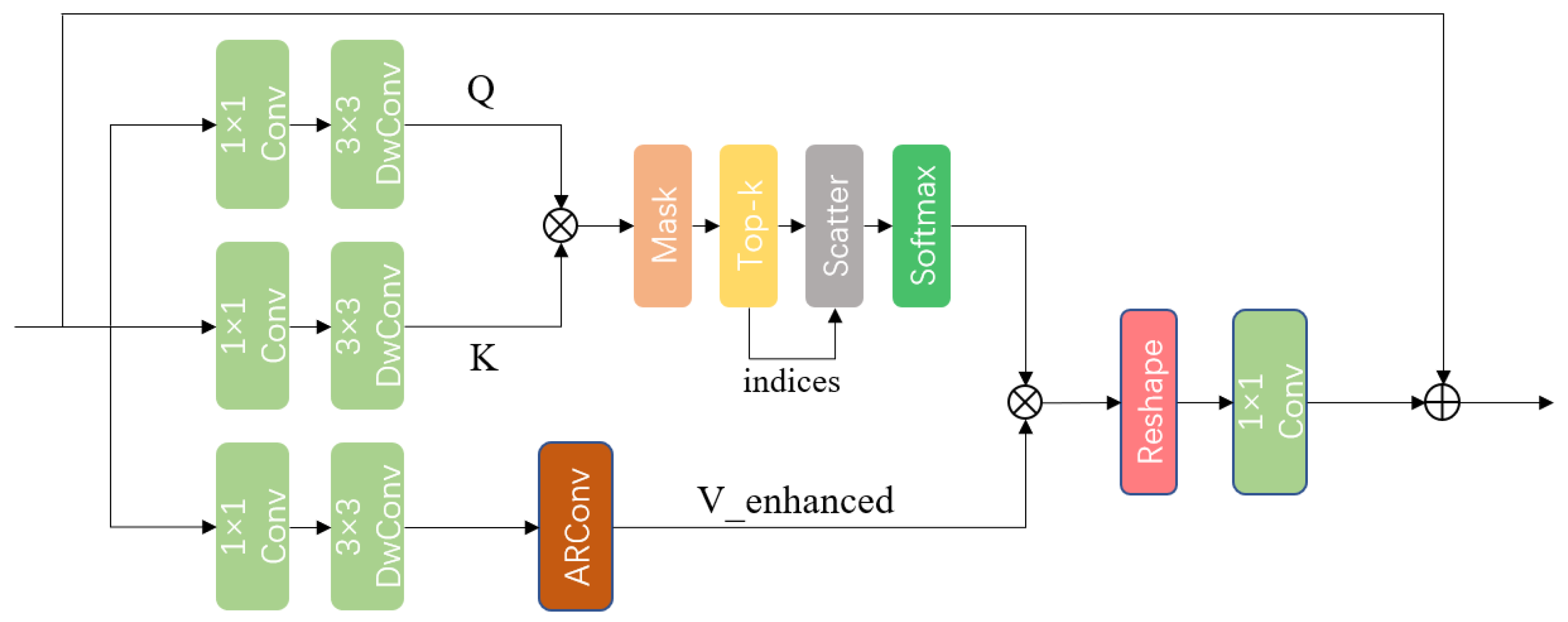
As shown in Figure 2, we first encode channel context via 1 × 1 convolution and 3 × 3 depthwise convolution, while introducing an ARConv module on the V branch to construct enhanced feature representation V enhanced :
V enhanced = ARConv ( V )
This module employs an adaptive rectangular convolution structure. The cross-channel attention computation retains the original flow: the transposed attention matrix M is computed by reshaping Q and K , followed by a dynamic top-k selection strategy preserving the top-k significant responses:
SparseAtt ( Q , K , V enhanced ) = softmax T k ( Q K T / d k ) V enhanced
where the T k ( · ) operator performs channel-wise adaptive filtering, retaining only the top-k maximum activations per row with normalization.
Here, the value matrix V is replaced by the enhanced version V enhanced with autoregressive context modeling. This design enables the model to capture long-range channel dependencies while maintaining computational efficiency.
Finally, multi-head attention fuses subspace features: outputs from multiple sparse attention heads are concatenated along the channel dimension, followed by a learnable linear projection matrix to generate the final representation.

3.1.3. ARConv

ARConv adaptively captures multi-scale features by dynamically learning geometric parameters and sampling strategies for convolution kernels [32]. Its structure is shown in Figure 3 and its core innovation lies in a three-stage mechanism:
(1)
Dynamic Kernel Parameter Learning
ARConv employs a dual-branch structure to predict height feature maps h R H × W × 1 and width feature maps w R H × W × 1 . Specifically, given input feature map X R H × W × C in : A shared feature extractor processes the input Dedicated Height Learner and Width Learner branches generate spatial parameters Sigmoid activation normalizes outputs, scaled by learnable modulation factors:
h = a h · σ ( f θ 1 ( X ) ) + b h
w = a w · σ ( f θ 2 ( X ) ) + b w
where a h , b h , a w , b w are learnable coefficients constraining kernel dimensions to preset physical ranges (e.g., h [ b h , a h + b h ] ). This enables each spatial position to dynamically adjust its receptive field based on local geometric properties.
(2)
Dynamic Sparse Sampling Mechanism
Using the learned height/width parameters, ARConv determines effective sampling points via adaptive selection:
k h = ϕ h ¯ n , k w = ϕ w ¯ m
where ϕ ( x ) = x [ x is even ] ensures an odd number of samples, and n , m are scaling coefficients. Sampling coordinates are generated through grid interpolation:
r i j = ( 2 i k h 1 ) h 0 2 k h , ( 2 j k w 1 ) w 0 2 k w
This produces a non-uniform sampling grid R R k h × k w × 2 , aligning kernel shape with target scales.
(3)
Affine Transformation for Spatial Adaptability
To enhance feature representation flexibility, ARConv incorporates the following learnable affine transformation:
Y = Conv ( S ; SK ) M + B
where: S R ( k h H ) × ( k w W ) × C in is the expanded sampled feature map M , B R H × W × C out are modulation matrix and bias terms predicted by subnetworks. It is worth noting that, rather than instantiating a full set of convolution weights at every spatial location, we use a shared kernel bank to produce a base response and apply a lightweight channel-wise affine modulation (scale and shift per channel) to adapt locally. This replaces a large 4-D weight tensor per location with just two channel vectors, drastically reducing the degrees of freedom and the risk of overfitting.
To provide an intuitive understanding of ARConv’s underlying mechanism, we visualize its geometry-adaptive behavior. As we can see in Figure 4, the convolution kernels adaptively modulate sampling pattern according to local geometry and scale by predicting position-wise height/width maps that deform a shared rectangular grid.

3.2. Semantic-Aware Discriminator

As shown in Figure 5, the Semantic-Aware Discriminator consists of a Semantic Feature Extractor and a Semantic-aware Fusion Block (SeFB) [33].
The Semantic Feature Extractor extracts multi-level semantic features from noise-free reference images I g t to provide semantic priors for the discriminator. We employ the ResNet-50 branch of the pre-trained vision-language model CLIP (CLIP-RN50), which was trained on large-scale image-text pairs and exhibits strong semantic representation capabilities. The RN50 architecture comprises four layers where feature resolution decreases through downsampling while semantic abstraction increases with layer depth. Experiments determined the third convolutional layer features as the optimal semantic source. This is mathematically expressed as follows:
S h = ϕ CLIP - RN 50 ( 3 ) ( I g t )
where ϕ ( 3 ) denotes the feature extraction function of CLIP-RN50’s third layer, and S h represents the semantic features.
The Semantic-aware Fusion Block dynamically integrates semantic features S h with image features f I (from either generated or real images) through semantic-conditioned feature modulation. The semantic features S h are first processed by a feature encoder composed of Group Normalization (GN), Layer Normalization (LN), and Self-Attention (SA) to generate a semantically enhanced query vector as follows:
Q = LN SA GN ( S h )
This procedure captures global contextual dependencies within semantic features via the self-attention mechanism. Concurrently, denoised image features f denoise and noise-free image features f gt are projected through convolutional layers to generate corresponding key-value pairs { K denoise , V denoise } and { K gt , V gt } .
Adaptive fusion of semantic and image features is achieved via the following cross-attention mechanism:
f ( ) att = Softmax Q · K ( ) d k V ( )
where d k is a scaling factor and ( ) denotes feature processing for different input branches ( d e n o i s e or g t ). It is worth noting that cross-attention explicitly aligns semantic priors with visual features via the query–key–value mechanism: semantic embeddings serve as queries while visual tokens act as keys/values, so the attention weights prioritize regions consistent with the semantics and suppress misleading correlations. For example, although water and vegetation may look similar at low resolution, a “water” query assigns higher weights to water surfaces and lower weights to vegetation, thereby mitigating semantic misalignment and achieving more consistent cross-modal alignment. To preserve original detail information, the attention features f ( ) att are further concatenated channel-wise with convolution-enhanced features Conv ( f ( ) ) , followed by nonlinear mapping, as follows:
f ( ) s = Conv GELU LN ( f ( ) att Conv ( f ( ) ) )
Here ⊕ indicates channel-wise concatenation, and the GELU activation function introduces smooth nonlinearity to enhance model expressiveness.

4. Experiment

4.1. Settings

4.1.1. Datasets

To enhance model generalization, our data sources comprise two components: public datasets and a custom-built private dataset.
Public Data Section: We utilize original images from the RRSSRD [34] and SECOND [35] datasets as our noise-free images. The RRSSRD is a remote sensing super-resolution dataset established by Dong et al. [34], and includes data from Worldview-2 and Gaofen-2, representing Xiamen City and Jinan City in China. The spatial resolution is 0.6 m, and each image comprises three channels: red (r), green (g) and blue (b). The original image size is 480 × 480 pixels. The SECOND dataset is a change detection dataset covering urban areas such as Hangzhou, Chengdu, and Shanghai in China. We use remote sensing images from this dataset, which are obtained from multi-platform, multi-sensor acquisition, thus ensuring data diversity and practical application value. The original image size is 512 × 512 pixels, and the spatial resolution is at a sub-meter level. It includes categories like non-vegetated surfaces, trees, low vegetation, water, buildings, and playgrounds, which cover typical change scenarios of natural and human activities. We crop the images along the center into 480 × 480 pixel sizes.
Private Data Section: We utilize images captured by the Jilin-1 satellite as our data source. These images have a spatial resolution of 0.5m and are comprised of RGB three channels. The images were taken from Hengyang City, which is situated in central-southern Hunan Province, China, with geographical coordinates ranging from 110°32′16″E–113°16′32″E and 26°07′05″N–27°28′24″N. The city features a complex and diverse terrain with land covers including urban areas, water bodies, farmland, and vegetation. Initially, we crop a full remote sensing image into numerous 480 × 480 pixel size images, discarding the remaining parts. Subsequently, we eliminate images containing large areas of zero-pixel values, considering these as invalid images.
By integrating both public and private data, the original images were corrupted using Additive White Gaussian Noise (AWGN). This process resulted in a total of 12,321 noise-clean image pairs, each measuring 480 × 480 pixels in size.

4.1.2. Implementation Details

In our research, the RATB quantity, AAL quantity, window size, and channel quantity are typically set to 6, 6, 8, and 180, respectively. During the training process, we employ the Adam optimizer [36] for optimization, with a batch size of 4. All denoising methods discussed in this paper are trained from scratch using an auxiliary training set. All experiments are conducted using Pytorch 2.5.1 and Python 3.10 on a server equipped with a 15-core, model Xeon(R) Platinum 8474C CPU and an NVIDIA GEFORCE RTX 4090 GPU (NVIDIA, Santa Clara, CA, USA) with 24G video memory.

4.1.3. Evaluation Metrics

Addressing the dual challenges of detail restoration and visual fidelity in the denoising task, this paper proposes a multi-dimensional evaluation system. This system encompasses pixel-level accuracy, structural consistency, and perceptual authenticity. The specific definitions of indicators and their calculation methods are detailed below.
In the image reconstruction task, the Mean Squared Error (MSE) evaluates the reconstruction fidelity by quantifying the mean of the squared differences between the corresponding pixels of the generated image X d e n o i s e d and the real high-resolution image X G T . Its mathematical expression is expressed as follows:
MSE = 1 H W i = 1 H j = 1 W ( X G T ( i , j ) X d e n o i s e d ( i , j ) ) 2
where H and W are the height and width of the image respectively. X G T ( i , j ) and X d e n o i s e d ( i , j ) represent the pixel values of the ground truth and the denoised image at the position ( i , j ) respectively.
The Peak Signal-to-Noise Ratio (PSNR) is constructed based on the Mean Squared Error (MSE). It measures the global fidelity of the reconstructed image by quantifying the ratio of the maximum signal intensity to the noise energy between the denoised image X d e n o i s e d and the real high-resolution image X G T . The calculation formula is expressed as follows:
PSNR = 10 · log 10 MAX I 2 MSE dB
where MAX I represents the maximum range of image pixel values (for example, 255 for 8-bit images), and MSE is the Mean Squared Error.
The Structural Similarity Index (SSIM) evaluates the perceptual consistency between the denoised image X d e n o i s e d and the real image X G T from three dimensions: luminance, contrast, and structural similarity by simulating the sensitivity of the human visual system to local structural information. The calculation formula is expressed as follows:
SSIM ( X G T , X d e n o i s e d ) = ( 2 μ X G T μ X d e n o i s e d + C 1 ) ( 2 σ X G T X d e n o i s e d + C 2 ) ( μ X G T 2 + μ X d e n o i s e d 2 + C 1 ) ( σ X G T 2 + σ X d e n o i s e d 2 + C 2 )
where μ X G T , μ X d e n o i s e d are the local means of the two images respectively, representing luminance information; σ X G T 2 , σ X d e n o i s e d 2 are the local variances, reflecting the contrast; σ X G T X d e n o i s e d is the covariance, describing the structural correlation; C 1 , C 2 are constant terms to avoid the denominator being zero, usually C 1 = ( 0.01 L ) 2 , C 2 = ( 0.03 L ) 2 , and L is the pixel dynamic range.
The Learned Perceptual Image Patch Similarity (LPIPS) measures the perceptual distance between the denoised image X d e n o i s e d and the real image X G T in the feature space by extracting high-order semantic features through a pre-trained deep neural network. The calculation process can be formalized as:
LPIPS ( X G T , X d e n o i s e d ) = l w l · ϕ l ( X G T ) ϕ l ( X d e n o i s e d ) 2 2
where ϕ l ( · ) represents the feature map of the l-th layer of the pre-trained network (such as VGG or AlexNet); w l is the learnable weight coefficient of each layer, calibrated through human visual preference data; · 2 is the L2 norm, quantifying the Euclidean distance of feature differences.
The Fréchet Inception Distance (FID) evaluates the overall realism and diversity of the generative model by calculating the distribution difference between the generated image set X d e n o i s e d = { X d e n o i s e d ( 1 ) , X d e n o i s e d ( 2 ) , , X d e n o i s e d ( N ) } and the real image set X G T = { X G T ( 1 ) , X G T ( 2 ) , , X G T ( N ) } in the deep feature space. Its mathematical expression is expressed as follows:
FID = μ X G T μ X d e n o i s e d 2 2 + Tr Σ X G T + Σ X d e n o i s e d 2 ( Σ X G T Σ X d e n o i s e d ) 1 / 2
where μ X G T , μ X d e n o i s e d R d are the feature mean vectors of the two sets ( d = 2048 corresponding to the ’pool3’ layer of Inception-v3); Σ X G T , Σ X d e n o i s e d R d × d are the feature covariance matrices; Tr ( · ) is the matrix trace operation, which quantifies the degree of match of the distribution structure.
In remote sensing image denoising, PSNR and SSIM are widely used to assess pixel-level fidelity. However, they primarily capture average per-pixel differences and can be insensitive to perceptual quality—particularly in high-noise or structurally complex scenes. By contrast, perceptual metrics such as LPIPS and FID are more sensitive to structural realism and fine textures, which are crucial for human interpretation and downstream applications (e.g., classification, target detection). Methods that score highly on PSNR/SSIM may still yield overly smooth results lacking fine detail. To mitigate this limitation, we report LPIPS and FID alongside PSNR/SSIM to evaluate realism and structural consistency in feature space and provide a more balanced assessment.In this work, our goal is to strike a balance between pixel-level fidelity and perceptual quality. We believe that striking a balance between pixel-level fidelity and perceptual quality is particularly important for practical remote sensing applications.

4.2. Comparisons with State-of-the-Art Algorithms

We compare the proposed SARFT-GAN method with several previous methods, including one local similarity-based method (BM3D [19]), two residual learning and convolutional neural network-based methods (DnCNN [23], BUIFD [37]), three Transformer-based methods (IDTransformer [38], SwinIR [39], CFAT [40]), one deep unfolding network-based method (DUMRN [41]), and one dual-branch method (DRANet [42]). Implementation codes were downloaded from the official websites of each method’s authors or designated code hosting platforms to ensure code accuracy and completeness. In our experiments, all methods used default parameter settings and were retrained using our remote sensing dataset. Evaluations were conducted separately for four different scenarios: building, farmland, vegetation, and water.
In evaluating the performance of denoising, experiments were conducted at three distinct noise intensity levels. During the image corruption phase, three specific noise intensities were introduced: σ = 15, σ = 25, and σ = 50. Here, σ denotes the standard deviation of Gaussian noise.

4.2.1. Quantitative Comparison

The quality of denoised images is quantitatively evaluated using four metrics: PSNR, SSIM, LPIPS, and FID. Table 1, Table 2 and Table 3 present a summary of the quantitative evaluation results across various methods and scenarios; with red indicating the highest performing method and blue signifying the second-best performance. It is evident from these tables that our method consistently achieves superior results on the FID image quality metric, irrespective of the noise level or scenario (a total of 12 conditions: 3 noise levels × 4 scenarios). In terms of LPIPS, our method outperforms in the majority of cases, with only three instances of secondary performance.While our method does not exhibit optimal performance for traditional pixel-level metrics (PSNR and SSIM) in every context, it consistently ranks among the top two. Notably, at a noise level of σ = 15, our approach achieves superior performance across all metrics in the vegetation scenario. The FID metric, in particular, is 1.91 lower than that of the next best method. This underscores our method’s marked proficiency in restoring intricate details of vegetation texture and scene semantics under minimal noise conditions. As noise levels escalate, our method maintains a robust performance edge, affirming its outstanding resistance to noise.Our results are competitive on PSNR/SSIM and strongly competitive on FID and LPIPS, indicating that the proposed SARFT-GAN better preserves realistic details and semantic consistency.

4.2.2. Qualitative Comparison

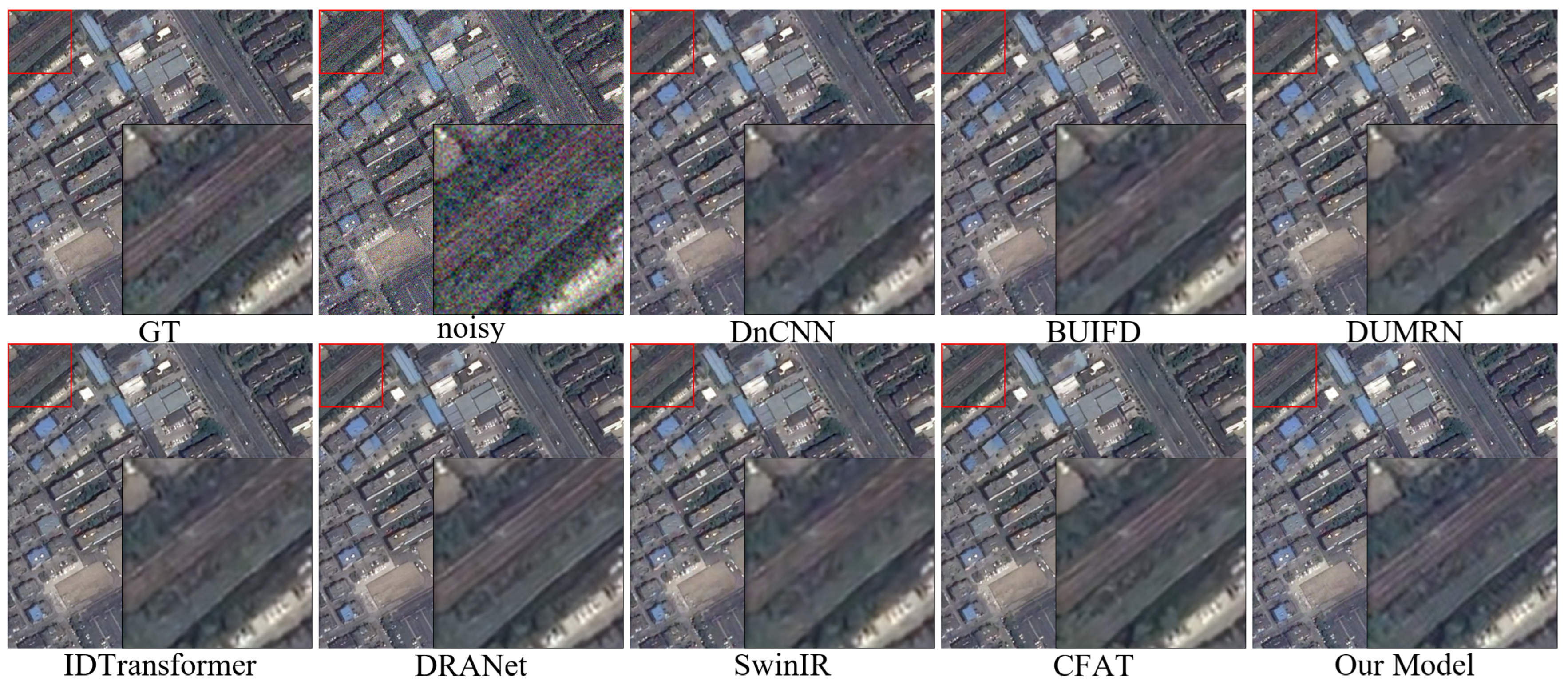
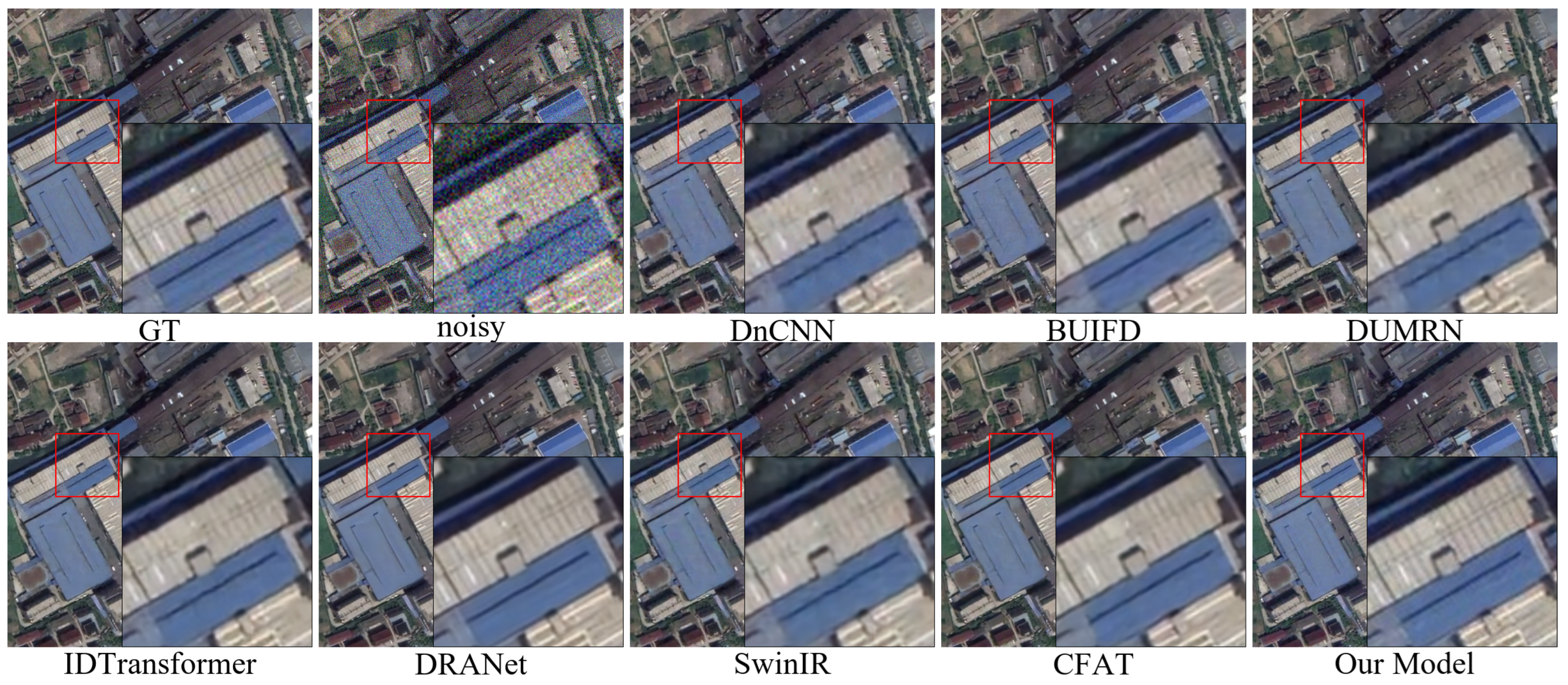
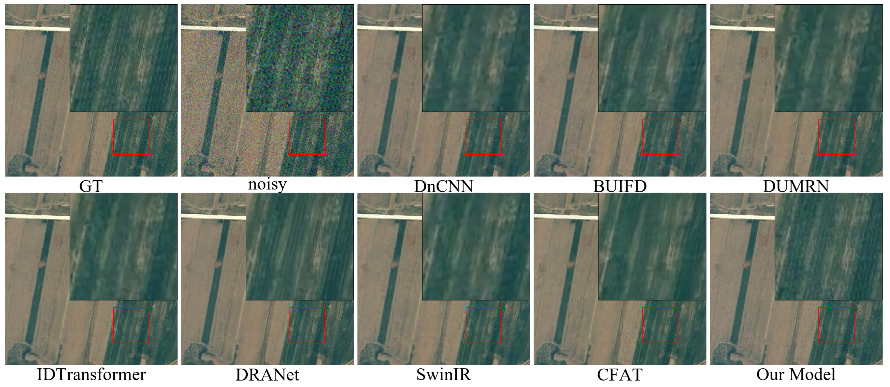
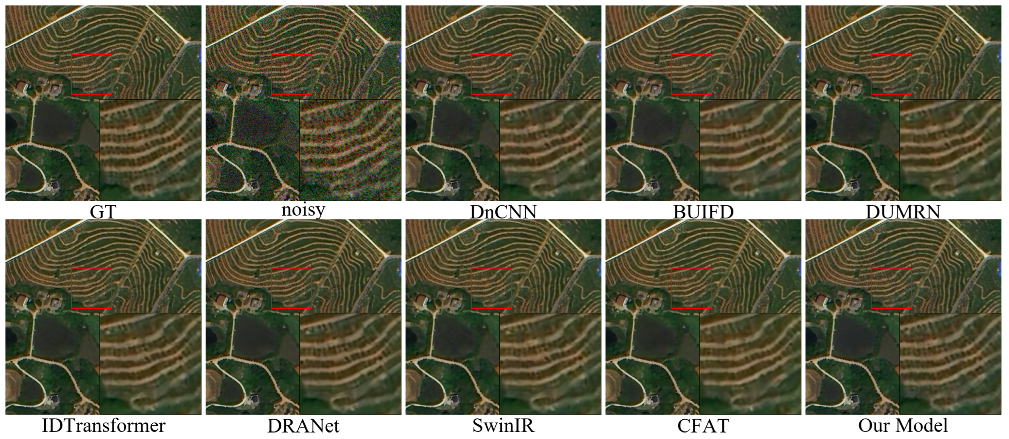
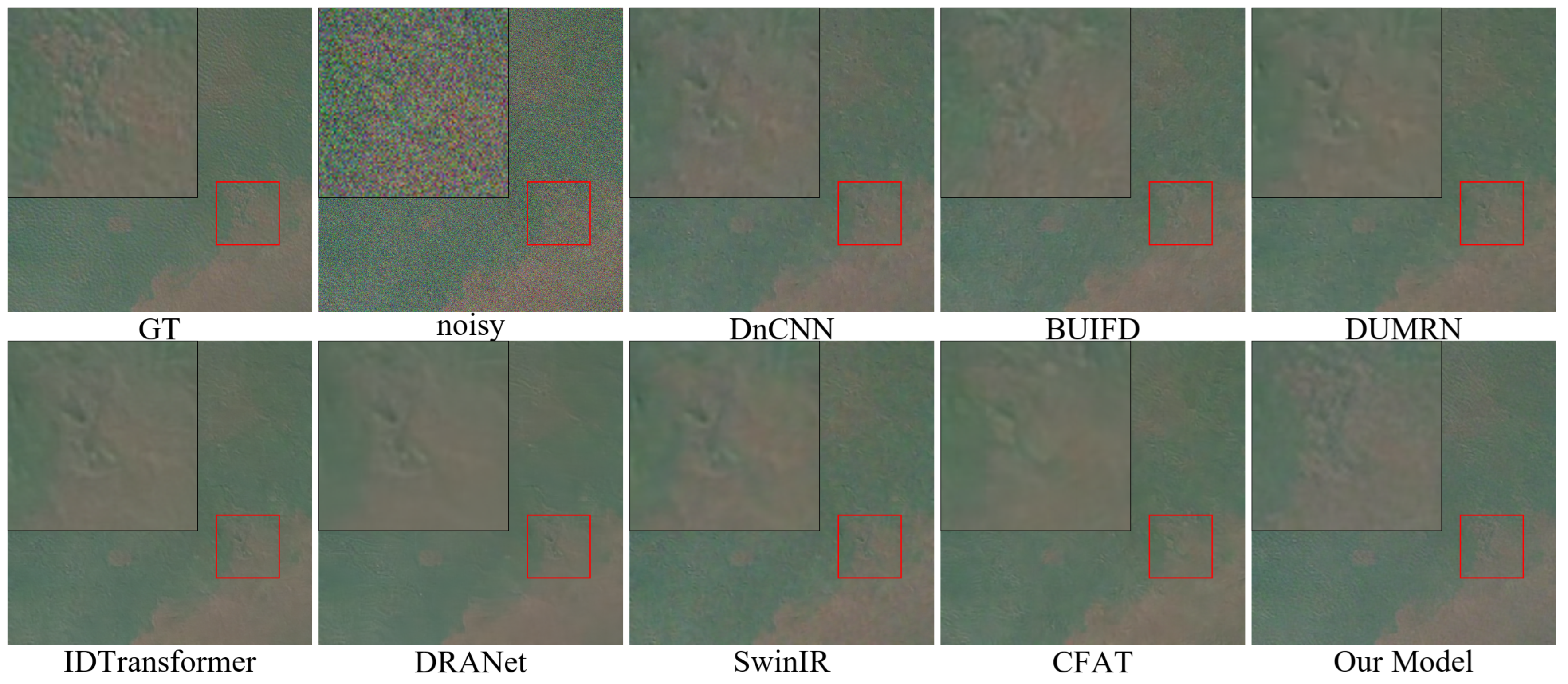
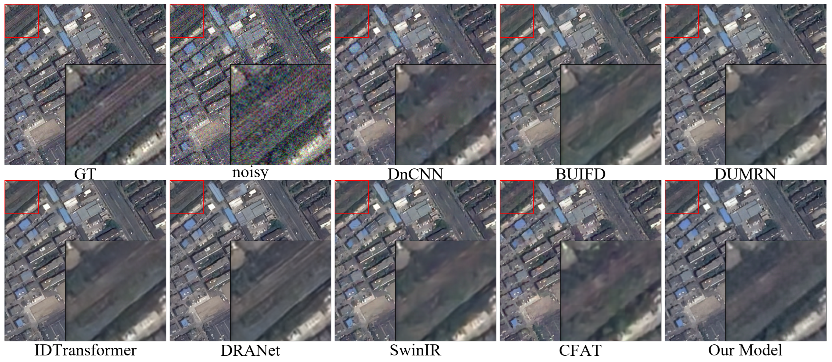
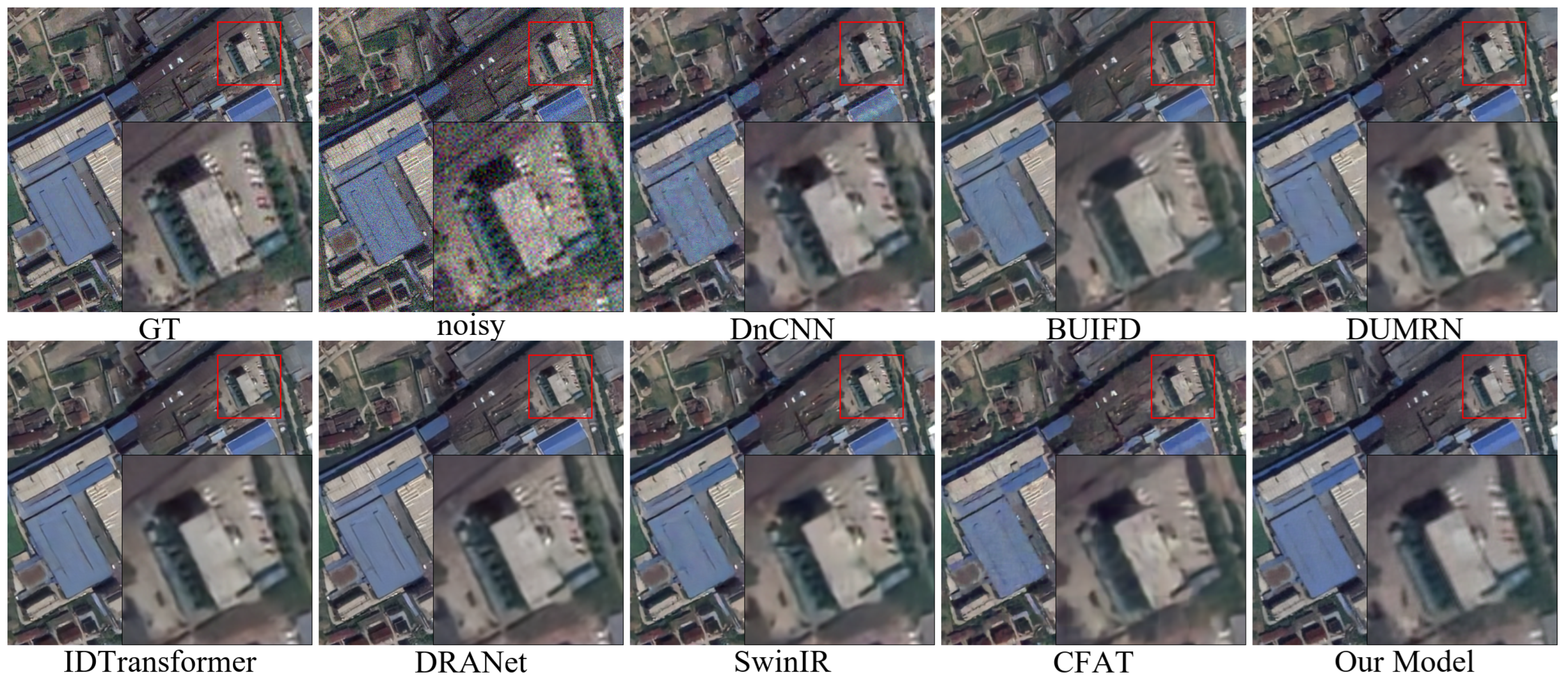
Figure 6, Figure 7, Figure 8, Figure 9 and Figure 10 illustrate the denoising effects of various methodologies under diverse scenarios at a noise level of σ = 25. All methods demonstrate adequate denoising capabilities when confronted with moderate noise levels. However, our method clearly surpasses others in terms of noise suppression, as evidenced by the intricate details of road lines in Figure 6 and roof features in Figure 7. While DnCNN and DUMRN exhibit some level of noise suppression, they fall short in terms of restored image quality, leaving noticeable smearing traces. BUIFD, IDTransformer, and SwinIR do not excessively smear, but they fall short in restoring texture details. On the other hand, DRANet and CFAT restores texture details effectively without any smearing, but the resultant image lacks a degree of realism and appears somewhat smoothed. Our proposed method masterfully balances noise suppression and texture detail restoration, yielding a more realistic and effective outcome than its counterparts. Figure 8 and Figure 9 depict the denoising effects at σ = 25 for farmland, vegetation, and water scenarios respectively. Consistent with conclusions drawn from the building scenario analysis, our method again proves superior in terms of realism and overall denoising results across different landscape details. This consistently showcases our method’s outstanding performance and robust generalization capability.
Figure 11 and Figure 12 display performance at a noise level of σ = 50. High-intensity noise presents substantial challenges. Notably, DnCNN, BUIFD, DUMRN, IDTransformer, SwinIR, and CFAT show significant distortion marked by pronounced smearing traces. In contrast, our method upholds detailed restoration with minimal distortion, even under such high-noise conditions. This underscores its robust strength.

4.3. Real-World Noisy Remote Sensing Images

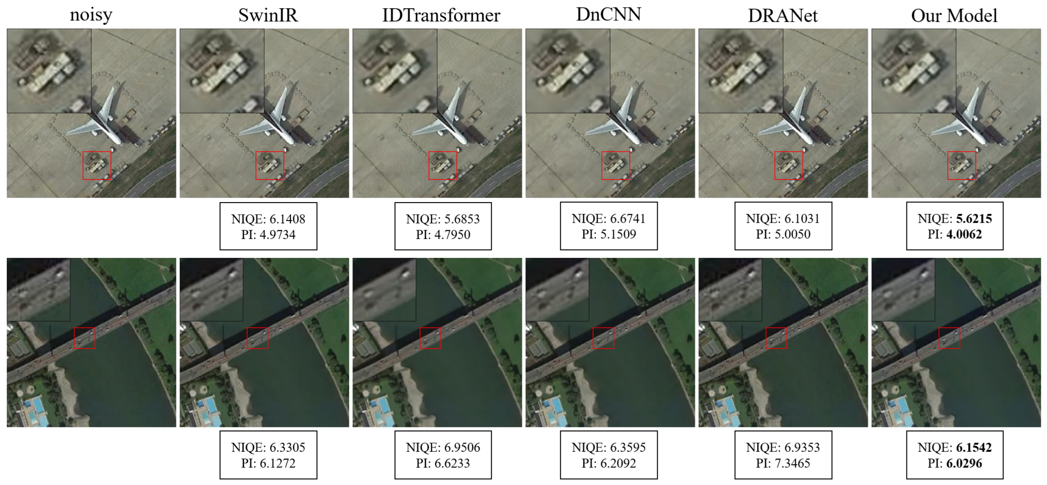
To further validate the effectiveness of the proposed method in restoring real-world noisy remote sensing images, we evaluate it on two real images from the NWPU-RESISC45 dataset [43]. Because these real images do not have matched clean references, PSNR and SSIM cannot be used in this subsection. Instead, we adopt two no-reference metrics: Natural Image Quality Evaluator (NIQE) [44] and Perceptual Index (PI) [45]. For both metrics, lower is better: NIQE assesses how closely an image conforms to natural scene statistics, and PI reflects overall perceptual quality. Although no-reference IQA metrics are not as precise as full-reference measures such as PSNR and SSIM, they still provide an objective assessment of image quality. As shown in Figure 13, our method exhibits clear advantages. It achieves the best NIQE and PI scores on all test images, indicating superior denoising performance. In terms of visual quality, SwinIR, IDTransformer and Our Model yield similarly pleasing results, which also explains their close NIQE and PI scores. Overall, these experiments demonstrate the effectiveness and reliability of our approach in practical applications.

4.4. Model Complexity and Runtime Comparison

We evaluated efficiency on an NVIDIA GeForce RTX 4090 (NVIDIA, Santa Clara, CA, USA). Table 4 compares our model with five recent methods (DnCNN, SwinIR, DRANet, IDTransformer, and CFAT) in terms of FLOPs, parameter count, and average per-image inference time; FLOPs and runtime were measured with 480×480 inputs. As shown in Table 4, the FLOPs and parameter count are comparable to those of transformer-based methods and relatively high; this follows from the added capacity of attention and enhanced convolutions, yet is acceptable. In contrast, our model is the second fastest in wall-clock inference time (behind only DnCNN), indicating solid practical efficiency. Overall, the method achieves a satisfactory efficiency.

4.5. Ablation Study

We conduct ablation studies to highlight the importance of each component in our model. Quantitative results are shown in Table 5. Results are averaged across test sets. All results were obtained under a noise level of σ = 15. Experimental groups include: (a) Model-1: Without ARConv attention (replaced with standard convolution) (b) Model-2: Without Top-k selection attention (c) Model-3: Without Semantic-Aware Discriminator (replaced with PatchGAN) (d) Model-4: Our proposed method (with both ARConv and Top-k selection attention) The table shows that combining Top-k and ARConv achieves optimal performance, while omitting either component degrades results. Model-1 performs slightly worse than Model-2, indicating that removing ARConv has a greater negative impact: removing ARConv harms content-adaptive feature formation and geometry-aligned aggregation, which has a larger impact on pixel-fidelity metrics than removing Top-k sparsification, because Top-k cannot compensate for the loss of ARConv’s geometry-aware receptive fields and enhanced value features. Model-3 outperforms Model-1 and Model-2 on PSNR and SSIM but underperforms them on LPIPS and FID, indicating that the Semantic-Aware Discriminator plays a larger role in improving perceptual quality in our method.

5. Discussion

It should be noted that our evaluation is mainly conducted on datasets which are primarily urban datasets. Although the proposed modules are not tied to specific scene categories, further validation on rural or mixed-land-cover datasets is necessary to fully assess generalization. We leave such evaluations—including agricultural and forested areas—for future work.
In addition to the above, our paper has other limitations. First, our method depends on a large quantity of remote sensing images for training, which may not be easy to obtain in many applications; future work can consider using unsupervised domain adaptation or few-shot learning techniques. Second, the Transformer contains many parameters and may place higher demands on hardware resources. Lightweight design also deserves further exploration.

6. Conclusions

This study introduces SARFT-GAN, an innovative generative adversarial network specifically designed for denoising optical remote sensing images. It achieves a synergistic optimization of noise suppression and detail preservation by overcoming the limitations inherent in traditional convolution operations, attention mechanisms, and discriminator design. The dynamic sampling mechanism, which is based on ARConv, allows for a flexible adjustment of the receptive field in accordance with target geometry. When combined with the Top-k sparse attention strategy, it effectively suppresses redundant interference from irrelevant features in global attention, thereby addressing issues of blurring in high-frequency texture regions. The semantically-aware discriminator further guides the generation process using semantic priors derived from pre-trained vision-language models, ensuring that texture reconstruction in complex scenes (e.g., vegetation, buildings) aligns with physical laws. Ablation studies have been conducted to validate the effectiveness of each SARFT-GAN component, with particular emphasis on the significant contribution of ARConv to performance. In conclusion, the proposed SARFT-GAN model demonstrates promising application potential in practical image denoising.

Author Contributions

Conceptualization, H.S.; methodology, H.S.; software, H.S.; validation, H.S.; formal analysis, H.S.; investigation, H.S.; resources, F.Y. and J.C.; data curation, R.D., G.S., H.Z. and F.C.; writing—original draft preparation, H.S.; writing—review and editing, F.Y.; visualization, H.S.; supervision, R.D., G.S., H.Z. and F.C.; project administration, F.Y. and J.C.; funding acquisition, F.Y. and J.C. All authors have read and agreed to the published version of the manuscript.

Funding

This research was funded by the National Key R&D Program of China (2022YFF1302700), the Emergency Open Competition Project of National Forestry and Grassland Administration (202303), and the Fundamental Research Funds for the Central Universities (ZZK202506).

Data Availability Statement

The data presented in this study are available upon request from the corresponding author due to confidentiality obligations stipulated in the participant consent agreements.

Conflicts of Interest

The authors declare no conflicts of interest.

References

  1. Feng, X.; Zhang, W.; Su, X.; Xu, Z. Optical remote sensing image denoising and super-resolution reconstructing using optimized generative network in wavelet transform domain. Remote Sens. 2021, 13, 1858. [Google Scholar] [CrossRef]
  2. Li, Q.; Huang, H.; Yu, W.; Jiang, S. Optimized views photogrammetry: Precision analysis and a large-scale case study in Qingdao. IEEE J. Sel. Top. Appl. Earth Obs. Remote Sens. 2023, 16, 1144–1159. [Google Scholar] [CrossRef]
  3. Zhu, Y.; Yang, G.; Yang, H.; Zhao, F.; Han, S.; Chen, R.; Zhang, C.; Yang, X.; Liu, M.; Cheng, J.; et al. Estimation of apple flowering frost loss for fruit yield based on gridded meteorological and remote sensing data in Luochuan, Shaanxi Province, China. Remote Sens. 2021, 13, 1630. [Google Scholar] [CrossRef]
  4. Qi, J.; Wan, P.; Gong, Z.; Xue, W.; Yao, A.; Liu, X.; Zhong, P. A self-improving framework for joint depth estimation and underwater target detection from hyperspectral imagery. Remote Sens. 2021, 13, 1721. [Google Scholar] [CrossRef]
  5. Xia, Z.; Li, Z.; Bai, Y.; Yu, J.; Adriano, B. Self-supervised learning for building damage assessment from large-scale xBD satellite imagery benchmark datasets. In Proceedings of the International Conference on Database and Expert Systems Applications, Vienna, Austria, 22–24 August 2022; Springer: Berlin/Heidelberg, Germany, 2022; pp. 373–386. [Google Scholar]
  6. Yuan, Q.; Zhang, Q.; Li, J.; Shen, H.; Zhang, L. Hyperspectral image denoising employing a spatial–spectral deep residual convolutional neural network. IEEE Trans. Geosci. Remote Sens. 2018, 57, 1205–1218. [Google Scholar] [CrossRef]
  7. Landgrebe, D.A.; Malaret, E. Noise in remote-sensing systems: The effect on classification error. IEEE Trans. Geosci. Remote Sens. 2007, GE-24, 294–300. [Google Scholar] [CrossRef]
  8. Foi, A.; Trimeche, M.; Katkovnik, V.; Egiazarian, K. Practical Poissonian-Gaussian noise modeling and fitting for single-image raw-data. IEEE Trans. Image Process. 2008, 17, 1737–1754. [Google Scholar] [CrossRef]
  9. Zhang, M.; Zhang, F.; Liu, Q.; Wang, S. VST-Net: Variance-stabilizing transformation inspired network for Poisson denoising. J. Vis. Commun. Image Represent. 2019, 62, 12–22. [Google Scholar] [CrossRef]
  10. Chen, J.; Chen, J.; Chao, H.; Yang, M. Image blind denoising with generative adversarial network based noise modeling. In Proceedings of the IEEE Conference on Computer Vision and Pattern Recognition, Salt Lake City, UT, USA, 18–23 June 2018; pp. 3155–3164. [Google Scholar]
  11. Cha, S.; Park, T.; Kim, B.; Baek, J.; Moon, T. GAN2GAN: Generative noise learning for blind denoising with single noisy images. arXiv 2019, arXiv:1905.10488. [Google Scholar]
  12. Huang, T.; Li, S.; Jia, X.; Lu, H.; Liu, J. Neighbor2neighbor: Self-supervised denoising from single noisy images. In Proceedings of the IEEE/CVF Conference on Computer Vision and Pattern Recognition, Nashville, TN, USA, 20–25 June 2021; pp. 14781–14790. [Google Scholar]
  13. Xue, S.; Qiu, W.; Liu, F.; Jin, X. Wavelet-based residual attention network for image super-resolution. Neurocomputing 2020, 382, 116–126. [Google Scholar] [CrossRef]
  14. Vaswani, A.; Shazeer, N.; Parmar, N.; Uszkoreit, J.; Jones, L.; Gomez, A.N.; Kaiser, Ł.; Polosukhin, I. Attention is all you need. Adv. Neural Inf. Process. Syst. 2017, 30, 6000–6010. [Google Scholar]
  15. Wang, P.; Wang, X.; Wang, F.; Lin, M.; Chang, S.; Li, H.; Jin, R. Kvt: K-nn attention for boosting vision transformers. In Proceedings of the European Conference on Computer Vision, Tel Aviv, Israel, 23–27 October 2022; Springer: Berlin/Heidelberg, Germany, 2022; pp. 285–302. [Google Scholar]
  16. Karras, T.; Laine, S.; Aittala, M.; Hellsten, J.; Lehtinen, J.; Aila, T. Analyzing and improving the image quality of stylegan. In Proceedings of the IEEE/CVF Conference on Computer Vision and Pattern Recognition, Seattle, WA, USA, 13–19 June 2020; pp. 8110–8119. [Google Scholar]
  17. Schonfeld, E.; Schiele, B.; Khoreva, A. A u-net based discriminator for generative adversarial networks. In Proceedings of the IEEE/CVF Conference on Computer Vision and Pattern Recognition, Seattle, WA, USA, 13–19 June 2020; pp. 8207–8216. [Google Scholar]
  18. Buades, A.; Coll, B.; Morel, J.M. A non-local algorithm for image denoising. In Proceedings of the 2005 IEEE Computer Society Conference on Computer Vision and Pattern Recognition (CVPR’05), San Diego, CA, USA, 20–25 June 2005; Volume 2, pp. 60–65. [Google Scholar]
  19. Dabov, K.; Foi, A.; Katkovnik, V.; Egiazarian, K. Image denoising by sparse 3-D transform-domain collaborative filtering. IEEE Trans. Image Process. 2007, 16, 2080–2095. [Google Scholar] [CrossRef]
  20. Aharon, M.; Elad, M.; Bruckstein, A. K-SVD: An algorithm for designing overcomplete dictionaries for sparse representation. IEEE Trans. Signal Process. 2006, 54, 4311–4322. [Google Scholar] [CrossRef]
  21. Gu, S.; Zhang, L.; Zuo, W.; Feng, X. Weighted nuclear norm minimization with application to image denoising. In Proceedings of the IEEE Conference on Computer Vision and Pattern Recognition, Columbus, OH, USA, 23–28 June 2014; pp. 2862–2869. [Google Scholar]
  22. Chang, S.G.; Yu, B.; Vetterli, M. Adaptive wavelet thresholding for image denoising and compression. IEEE Trans. Image Process. 2000, 9, 1532–1546. [Google Scholar] [CrossRef]
  23. Zhang, K.; Zuo, W.; Chen, Y.; Meng, D.; Zhang, L. Beyond a gaussian denoiser: Residual learning of deep cnn for image denoising. IEEE Trans. Image Process. 2017, 26, 3142–3155. [Google Scholar] [CrossRef] [PubMed]
  24. Zhang, K.; Zuo, W.; Zhang, L. FFDNet: Toward a fast and flexible solution for CNN-based image denoising. IEEE Trans. Image Process. 2018, 27, 4608–4622. [Google Scholar] [CrossRef] [PubMed]
  25. Anwar, S.; Barnes, N. Real image denoising with feature attention. In Proceedings of the IEEE/CVF International Conference on Computer Vision, Seoul, Republic of Korea, 27 October–2 November 2019; pp. 3155–3164. [Google Scholar]
  26. Guo, S.; Yan, Z.; Zhang, K.; Zuo, W.; Zhang, L. Toward convolutional blind denoising of real photographs. In Proceedings of the IEEE/CVF Conference on Computer Vision and Pattern Recognition, Long Beach, CA, USA, 15–20 June 2019; pp. 1712–1722. [Google Scholar]
  27. Zheng, Y.; Su, J.; Zhang, S.; Tao, M.; Wang, L. Dehaze-AGGAN: Unpaired remote sensing image dehazing using enhanced attention-guide generative adversarial networks. IEEE Trans. Geosci. Remote Sens. 2022, 60, 1–13. [Google Scholar] [CrossRef]
  28. Wang, Y.; Chang, D.; Zhao, Y. A new blind image denoising method based on asymmetric generative adversarial network. IET Image Process. 2021, 15, 1260–1272. [Google Scholar] [CrossRef]
  29. Gulrajani, I.; Ahmed, F.; Arjovsky, M.; Dumoulin, V.; Courville, A.C. Improved training of wasserstein gans. Adv. Neural Inf. Process. Syst. 2017, 30, 5769–5779. [Google Scholar]
  30. Han, Z.; Shangguan, H.; Zhang, X.; Cui, X.; Wang, Y. A coarse-to-fine multi-scale feature hybrid low-dose CT denoising network. Signal Process. Image Commun. 2023, 118, 117009. [Google Scholar] [CrossRef]
  31. Jin, M.; Wang, P.; Li, Y. Hya-gan: Remote sensing image cloud removal based on hybrid attention generation adversarial network. Int. J. Remote Sens. 2024, 45, 1755–1773. [Google Scholar] [CrossRef]
  32. Wang, X.; Zheng, Z.; Shao, J.; Duan, Y.; Deng, L.J. Adaptive Rectangular Convolution for Remote Sensing Pansharpening. In Proceedings of the Computer Vision and Pattern Recognition Conference, Nashville, TN, USA, 10–17 June 2025; pp. 17872–17881. [Google Scholar]
  33. Li, B.; Li, X.; Zhu, H.; Jin, Y.; Feng, R.; Zhang, Z.; Chen, Z. Sed: Semantic-aware discriminator for image super-resolution. In Proceedings of the IEEE/CVF Conference on Computer Vision and Pattern Recognition, Seattle, WA, USA, 16–22 June 2024; pp. 25784–25795. [Google Scholar]
  34. Dong, R.; Zhang, L.; Fu, H. RRSGAN: Reference-based super-resolution for remote sensing image. IEEE Trans. Geosci. Remote Sens. 2021, 60, 1–17. [Google Scholar] [CrossRef]
  35. Yang, K.; Xia, G.S.; Liu, Z.; Du, B.; Yang, W.; Pelillo, M.; Zhang, L. Semantic change detection with asymmetric Siamese networks. arXiv 2020, arXiv:2010.05687. [Google Scholar]
  36. Kingma, D.P.; Ba, J. Adam: A method for stochastic optimization. arXiv 2014, arXiv:1412.6980. [Google Scholar]
  37. El Helou, M.; Süsstrunk, S. Blind universal Bayesian image denoising with Gaussian noise level learning. IEEE Trans. Image Process. 2020, 29, 4885–4897. [Google Scholar] [CrossRef] [PubMed]
  38. Shen, Z.; Qin, F.; Ge, R.; Wang, C.; Zhang, K.; Huang, J. IDTransformer: Infrared image denoising method based on convolutional transposed self-attention. Alex. Eng. J. 2025, 110, 310–321. [Google Scholar] [CrossRef]
  39. Liang, J.; Cao, J.; Sun, G.; Zhang, K.; Van Gool, L.; Timofte, R. Swinir: Image restoration using swin transformer. In Proceedings of the IEEE/CVF International Conference on Computer Vision, Montreal, BC, Canada, 11–17 October 2021; pp. 1833–1844. [Google Scholar]
  40. Ray, A.; Kumar, G.; Kolekar, M.H. Cfat: Unleashing triangular windows for image super-resolution. In Proceedings of the IEEE/CVF Conference on Computer Vision and Pattern Recognition, Seattle, WA, USA, 16–22 June 2024; pp. 26120–26129. [Google Scholar]
  41. Xu, J.; Yuan, M.; Yan, D.M.; Wu, T. Deep unfolding multi-scale regularizer network for image denoising. Comput. Vis. Media 2023, 9, 335–350. [Google Scholar] [CrossRef]
  42. Wu, W.; Liu, S.; Xia, Y.; Zhang, Y. Dual residual attention network for image denoising. Pattern Recognit. 2024, 149, 110291. [Google Scholar] [CrossRef]
  43. Cheng, G.; Han, J.; Lu, X. Remote sensing image scene classification: Benchmark and state of the art. Proc. IEEE 2017, 105, 1865–1883. [Google Scholar] [CrossRef]
  44. Mittal, A.; Soundararajan, R.; Bovik, A.C. Making a “completely blind” image quality analyzer. IEEE Signal Process. Lett. 2012, 20, 209–212. [Google Scholar] [CrossRef]
  45. Wang, X.; Yu, K.; Wu, S.; Gu, J.; Liu, Y.; Dong, C.; Qiao, Y.; Change Loy, C. Esrgan: Enhanced super-resolution generative adversarial networks. In Proceedings of the European Conference on Computer Vision (ECCV) Workshops, Munich, Germany, 8–14 September 2018. [Google Scholar]
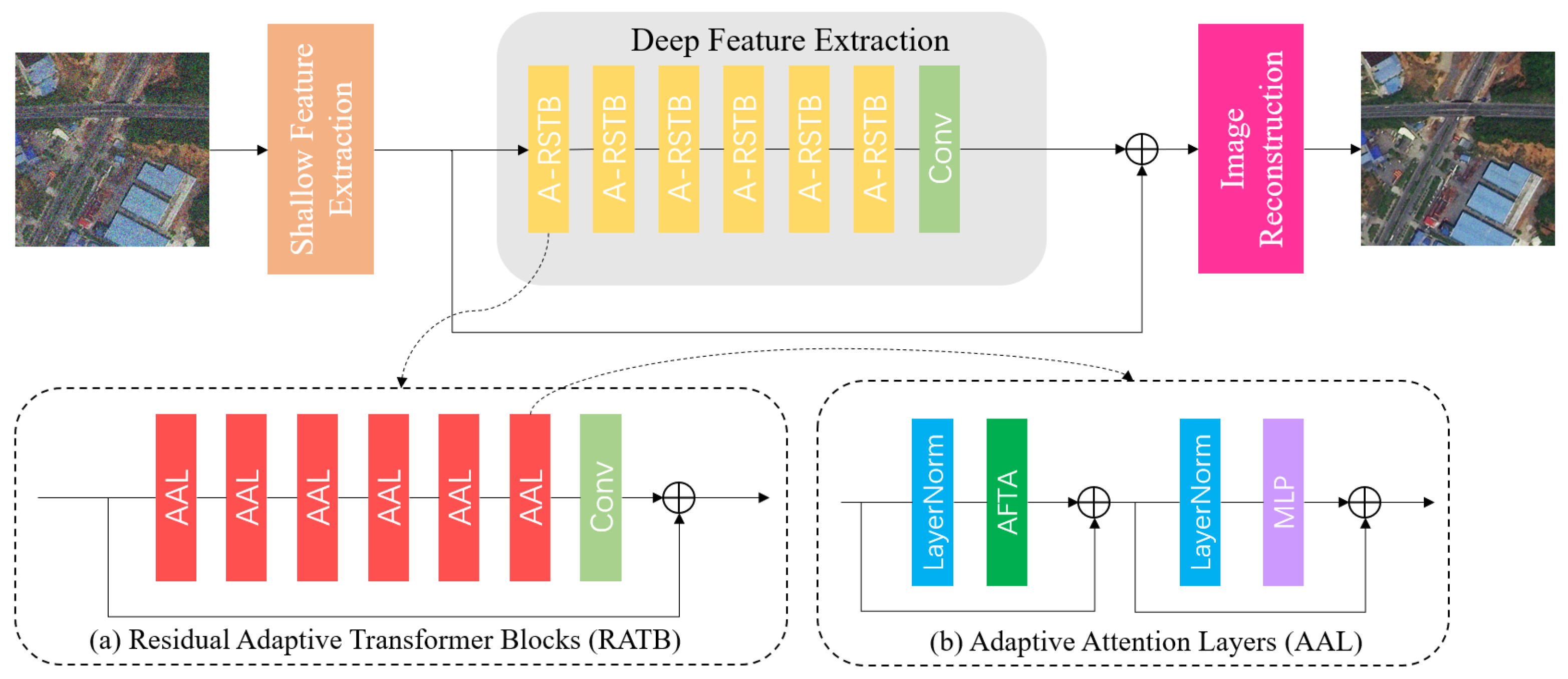
Figure 1. Overall framework of our SARFT-GAN.Models include the shallow feature extraction module, deep feature extraction module and image reconstruction module.
Remotesensing 17 03114 g001
Figure 2. Flowchart of ARConv Fused Top-k Attention. DWConv refers to the depth-wise convolution.
Remotesensing 17 03114 g002
Figure 3. Flowchart of ARConv, This module consists of three main parts. The first part addresses the learning process of the convolution kernel’s height and width. The second part focuses on the selection process for the number of sampling points of the convolution kernel. The third part simulates the generation process of the sampling map.
Remotesensing 17 03114 g003
Figure 4. Visualization of ARConv’s geometry-adaptive sampling. Left: a remote sensing image. Right: on the zoomed patches we overlay the rectangular sparse sampling lattice.
Remotesensing 17 03114 g004
Figure 5. Flowchart of Semantic-Aware Discriminator.
Remotesensing 17 03114 g005
Figure 6. The visual demonstration showcases the effectiveness of diverse denoising methodologies applied to Example 1 of the building test set corrupted by additive white Gaussian noise (AWGN) with σ = 25 .
Remotesensing 17 03114 g006
Figure 7. The visual demonstration showcases the effectiveness of diverse denoising methodologies applied to Example 2 of the building test set corrupted by additive white Gaussian noise (AWGN) with σ = 25 .
Remotesensing 17 03114 g007
Figure 8. The visual demonstration showcases the effectiveness of diverse denoising methodologies applied to Example 1 of the farmland test set corrupted by additive white Gaussian noise (AWGN) with σ = 25 .
Remotesensing 17 03114 g008
Figure 9. The visual demonstration showcases the effectiveness of diverse denoising methodologies applied to Example 1 of the vegetation test set corrupted by additive white Gaussian noise (AWGN) with σ = 25 .
Remotesensing 17 03114 g009
Figure 10. The visual demonstration showcases the effectiveness of diverse denoising methodologies applied to Example 1 of the water test set corrupted by additive white Gaussian noise (AWGN) with σ = 25 .
Remotesensing 17 03114 g010
Figure 11. The visual demonstration showcases the effectiveness of diverse denoising methodologies applied to Example 1 of the building test set corrupted by additive white Gaussian noise (AWGN) with σ = 50 .
Remotesensing 17 03114 g011
Figure 12. The visual demonstration showcases the effectiveness of diverse denoising methodologies applied to Example 2 of the building test set corrupted by additive white Gaussian noise (AWGN) with σ = 50 .
Remotesensing 17 03114 g012
Figure 13. Comparison of the performance of different models in NWPU-RESISC45 images.
Remotesensing 17 03114 g013
Table 1. Quantitative results of different methods in four scenarios with additive white Gaussian noise ( σ = 15 ). ↑ indicates that higher values are better and ↓ indicates that lower values are better. The best results are marked in red, while the second-best results are marked in blue.
ScenarioMetricBM3DDnCNNBUIFDDUMRNDRANetIDTransformerSwinIRCFATOur Model
BuildingPSNR ↑35.5436.7533.9436.7137.3236.8036.5536.0436.82
SSIM ↑0.93590.94900.94880.94810.95530.94940.95280.94590.9563
LPIPS ↓0.20460.14500.18220.14900.12410.14270.13340.14960.1220
FID ↓86.2427.5039.3130.4028.1932.0528.2130.3421.32
FarmlandPSNR ↑37.6538.1934.0638.2539.2038.5538.9537.5138.45
SSIM ↑0.92250.93440.93340.92950.94540.93580.93630.92940.9385
LPIPS ↓0.26680.21830.24860.22690.17890.21060.19890.22300.1770
FID ↓128.8768.1677.8272.6258.7368.4465.6271.0551.85
VegetationPSNR ↑36.2337.6534.6337.5637.3237.6637.8636.6337.99
SSIM ↑0.91560.94050.93850.93800.93910.93950.94290.93620.9446
LPIPS ↓0.25070.18470.20790.19020.16100.18260.17800.18240.1537
FID ↓93.9341.9150.3242.4040.7244.5141.7840.0338.12
WaterPSNR ↑42.3342.6138.9642.0643.6042.7743.3039.6942.34
SSIM ↑0.96330.96440.95980.96220.97050.96420.96360.96170.9659
LPIPS ↓0.28360.29430.35820.28180.24870.32170.31130.28920.1924
FID ↓161.2482.77106.6280.40111.28107.47117.7089.5259.24
Table 2. Quantitative results of different methods in four scenarios with additive white Gaussian noise ( σ = 25 ). ↑ indicates that higher values are better and ↓ indicates that lower values are better. The best results are marked in red, while the second-best results are marked in blue.
ScenarioMetricBM3DDnCNNBUIFDDUMRNDRANetIDTransformerSwinIRCFATOur Model
BuildingPSNR ↑32.7333.3934.0234.0134.3334.1433.9134.2134.64
SSIM ↑0.89140.90760.90840.91400.92620.91620.91220.91950.9170
LPIPS ↓0.28420.22730.20960.22330.18710.20550.22940.20680.1993
FID ↓140.7460.9352.5965.8964.7058.7176.2667.1748.02
FarmlandPSNR ↑35.3335.7736.0735.9736.6836.2835.9236.4436.98
SSIM ↑0.87950.88770.89780.89000.91750.89990.89150.90640.8990
LPIPS ↓0.34560.31300.28920.31060.26950.27670.31310.27770.2441
FID ↓164.58118.73107.23123.45106.76116.13120.53121.16101.74
VegetationPSNR ↑33.3534.7434.6234.4634.9235.0634.8034.9135.25
SSIM ↑0.84870.89000.88870.89390.90390.89930.89120.89720.8946
LPIPS ↓0.34000.26650.25830.27120.23770.24440.27600.26210.2352
FID ↓145.5173.9779.2675.8577.8672.5793.0282.9271.19
WaterPSNR ↑40.4140.1939.9140.6741.7441.2440.1240.8141.89
SSIM ↑0.95400.95080.95330.95520.96040.95780.95210.95810.9597
LPIPS ↓0.34890.39320.37560.38280.29550.34890.36730.38770.2353
FID ↓196.00128.62169.29141.43172.15173.04145.18180.15102.88
Table 3. Quantitative results of different methods in four scenarios with additive white Gaussian noise ( σ = 50 ). ↑ indicates that higher values are better and ↓ indicates that lower values are better. The best results are marked in red, while the second-best results are marked in blue.
ScenarioMetricBM3DDnCNNBUIFDDUMRNDRANetIDTransformerSwinIRCFATOur Model
BuildingPSNR ↑28.7929.4030.0130.6030.7830.9430.6930.4231.23
SSIM ↑0.79510.81440.84210.84530.85780.85430.84550.84010.8648
LPIPS ↓0.41440.36330.31390.33360.27470.31120.32680.33470.3072
FID ↓210.23127.03138.30138.30113.62117.68145.56113.2197.37
FarmlandPSNR ↑32.3732.9332.8733.3934.0833.8733.4833.0934.27
SSIM ↑0.81530.82430.83430.83480.86450.84640.83370.83250.8632
LPIPS ↓0.46430.42680.39640.40350.33760.38970.40990.40390.3820
FID ↓251.98188.32186.64189.70174.61179.79210.20184.45167.58
VegetationPSNR ↑29.4931.4029.6331.6431.9831.8131.5531.3931.95
SSIM ↑0.73350.79230.76670.80100.80730.80920.79500.80050.8193
LPIPS ↓0.46010.39990.41760.38950.35440.35340.39430.36600.3478
FID ↓223.78158.42183.06166.36142.29132.30170.74127.64126.88
WaterPSNR ↑34.2036.9833.0138.2539.3639.1338.4637.7539.03
SSIM ↑0.93680.92530.93700.92820.94870.94030.94160.93860.9408
LPIPS ↓0.43590.47520.38960.44480.33150.36070.40320.40570.3044
FID ↓259.41220.70222.97256.40200.96188.22223.35218.11162.06
Table 4. Computational cost and efficiency comparison.
MetricDnCNNSwinIRDRANetIDTransformerCFATOur Model
FLOPs [G]129.082644.222082.41486.154978.762867.39
Params [M]0.5611.461.6218.5321.4911.56
Average Inference Time [ms]1.51243.9188236.28123.225.8
Table 5. Ablation analysis of SARFT-GAN with different components. ↑ indicates that higher values are better and ↓ indicates that lower values are better.
MethodPSNR ↑SSIM ↑LPIPS ↓FID ↓
Model-137.220.94230.172250.64
Model-237.930.94830.169247.58
Model-337.950.94960.184352.35
Model-4 (Our)38.910.95130.161342.63
Disclaimer/Publisher’s Note: The statements, opinions and data contained in all publications are solely those of the individual author(s) and contributor(s) and not of MDPI and/or the editor(s). MDPI and/or the editor(s) disclaim responsibility for any injury to people or property resulting from any ideas, methods, instructions or products referred to in the content.