Article

Impacts of Land Use Patterns on Flood Risk in the Chang-Zhu-Tan Urban Agglomeration, China

1
School of Public Policy and Management, China University of Mining and Technology, Xuzhou 221116, China
2
Department of Geography, Vrije Universiteit Brussel, 1050 Brussels, Belgium
*
Author to whom correspondence should be addressed.
Remote Sens. 2025, 17(16), 2889; https://doi.org/10.3390/rs17162889
Submission received: 2 July 2025 / Revised: 10 August 2025 / Accepted: 18 August 2025 / Published: 19 August 2025

Abstract

Flood risk assessment is an effective tool for disaster prevention and mitigation. As land use is a key factor influencing flood disasters, studying the impact of different land use patterns on flood risk is crucial. This study evaluates flood risk in the Chang-Zhu-Tan (CZT) urban agglomeration by selecting 17 socioeconomic and natural environmental factors within a risk assessment framework encompassing hazard, exposure, vulnerability, and resilience. Additionally, the Patch-Generating Land Use Simulation (PLUS) and multilayer perceptron (MLP)/Bayesian network (BN) models were coupled to predict flood risks under three future land use scenarios: natural development, urban construction, and ecological protection. This integrated modeling framework combines MLP’s high-precision nonlinear fitting with BN’s probabilistic inference, effectively mitigating prediction uncertainty in traditional single-model approaches while preserving predictive accuracy and enhancing causal interpretability. The results indicate that high-risk flood zones are predominantly concentrated along the Xiang River, while medium-high- and medium-risk areas are mainly distributed on the periphery of high-risk zones, exhibiting a gradient decline. Low-risk areas are scattered in mountainous regions far from socioeconomic activities. Simulating future land use using the PLUS model with a Kappa coefficient of 0.78 and an overall accuracy of 0.87. Under all future scenarios, cropland decreases while construction land increases. Forestland decreases in all scenarios except for ecological protection, where it expands. In future risk predictions, the MLP model achieved a high accuracy of 97.83%, while the BN model reached 87.14%. Both models consistently indicated that the flood risk was minimized under the ecological protection scenario and maximized under the urban construction scenario. Therefore, adopting ecological protection measures can effectively mitigate flood risks, offering valuable guidance for future disaster prevention and mitigation strategies.

1. Introduction

As urbanization accelerates, natural disasters have become increasingly frequent, with urban flooding emerging as a recurring phenomenon. At the United Nations Water Conference (UNWC) in March 2023, UN Secretary-General António Guterres highlighted that three-quarters of all global natural disasters are water-related. Floods rank as the most devastating of all natural disasters in terms of vulnerability and impact, often affecting multiple regions simultaneously. According to the Emergency Events Database (EM-DAT), floods affected approximately 270 million people worldwide between 2000 and 2018, resulting in nearly 100,000 fatalities and economic losses totaling USD 640 billion [1]. And there is an inextricable link between land, as a carrier of human production and life, and flooding [2]. First, extensive land has been allocated for housing, roads, infrastructure, and industrial facilities, replacing permeable surfaces with impervious concrete cover. This prevents rainwater infiltration during precipitation events, significantly increasing flood risks. Second, variations in land use types—each with distinct socioeconomic values—result in uneven population and economic distribution across regions, further influencing flood vulnerability. Additionally, excessive deforestation and vegetation loss diminish soil water retention capacity, promoting soil loosening and erosion, which exacerbates flood hazards. Consequently, scientifically informed and sustainable land use planning is essential for effective flood mitigation [3].
Flood risk is generally considered to be a collection of hazards, exposures, and vulnerabilities [4]. Several scholars conceptualize risk as a function of both hazard and vulnerability, positing that risk emerges from the interaction between physical threats and societal susceptibility [5]. With ongoing advancements in urban disaster prevention capabilities, a growing body of scholarship now integrates resilience into risk assessment frameworks to enable more comprehensive evaluations of flood risk [6].
In recent years, numerous studies have been conducted to assess urban flooding risks, primarily employing three approaches: the historical disaster method, the index system method, and the scenario simulation method. Among these, the historical disaster method is relatively straightforward to implement but suffers from limited accuracy. For instance, Zhang et al. utilized natural disaster census data to evaluate agricultural disaster risks in Jilin Province, China, demonstrating the method’s practical application while highlighting its constraints [7]. Benito et al. analyzed the flood characteristics of the Douro River in Spain based on historical flood data [8]. The scenario simulation method primarily employs hydrodynamic modeling to assess flood risk, establishing specific scenarios to evaluate potential impacts under varying conditions. For instance, Mainguenaud et al. utilized a 1D/2D hydrodynamic model to simulate the consequences of levee failure [9]. Similarly, Liu et al. integrated Monte Carlo simulation with gridded population exposure and vulnerability data to develop a composite flood risk index, enabling risk assessment and prediction across different socioeconomic scenarios [10]. Other applications include the work of Tanim et al., who used the SWMM model for flood modeling [11], and Zischg et al., who analyzed river flood exposure in Switzerland by combining topographic data with the two-dimensional model BASEMENT v2.6 [12]. Further advancing the methodology, Zhao et al. coupled the 1D SWMM model with the 2D MIKE21 model to simulate river network flood risks under different recurrence intervals, leveraging remotely sensed data to map inundation extent and distribution in Cangzhou City, China [13]. The primary advantage of the scenario simulation method lies in its capacity to assess and predict flood risks under diverse future conditions, including varying return periods, land use practices, and climate change pathways. By simulating these scenarios, this approach enables proactive disaster preparedness and mitigation planning, offering valuable insights for long-term urban resilience strategies. The indicator system method, also referred to as the multi-criteria decision analysis (MCDA) approach, constructs a flood risk assessment framework tailored to the study area’s flood characteristics, natural geography, and socioeconomic conditions. This method systematically evaluates flood risk by integrating relevant indicators across multiple dimensions. For example, Bhuyan et al. selected an indicator system based on hazard and vulnerability to assess flood risk in the Nagaon region [14]. Similarly, Chen et al. evaluated flash flood risk by selecting key factors from three critical aspects—disaster-causing factors, disaster-predisposing environments, and disaster-bearing bodies—after first validating the accuracy of China’s flash flood hydrological modeling system [15]. MCDA offers greater flexibility, though its accuracy largely hinges on the selection of the indicator system and the determination of indicator weights. Scholars have progressively refined the risk assessment indicator system, initially focusing on natural geographic factors and later incorporating socioeconomic factors, urban resilience metrics, and other relevant dimensions. Notably, the growing application of social media big data in risk assessment has further enhanced the reliability of results [16,17]. Regarding weight determination, methodological advancements—from single subjective or objective approaches to simple multi-method combinations, and more recently, to machine learning techniques such as Random Forest (RF)—have significantly improved assessment accuracy [18].
Recent advances in data-driven and machine learning (ML) methods have introduced new possibilities for disaster risk assessment. Lu et al. developed a BN-GIS model, leveraging GIS’s spatial analysis capabilities and Bayesian networks’ probabilistic inference to assess flood hazards in Yinchuan City [19]. Wang et al. proposed a heterogeneous ensemble learning technique integrating multiple algorithms to evaluate flood risk in Shenzhen, revealing a strong correlation between urban development and heightened flood risk [20]. When applying ML or deep learning to risk assessment, accuracy is a critical consideration. For instance, Wei et al. compared five ML models for extreme rainfall-induced flooding, reporting accuracies exceeding 80%, with CatBoost achieving 95% accuracy [21]. Other ML approaches—such as K-means, BP neural networks, SVM, RF, and XGBoost—have also demonstrated high predictive performance in risk assessment [22,23,24]. Beyond accuracy, interpretability remains a key objective in ML applications. While conventional models often rely on post hoc techniques (e.g., SHAP, PDP) to enhance interpretability, BN models inherently provide full transparency due to their probabilistic graphical structure [25,26].
To address the challenges posed by uncertain future conditions, it is crucial to simulate potential development scenarios and evaluate flood risks under varying conditions. Such assessments hold strategic importance for advancing sustainable urban development. Integrating machine learning with scenario simulation can enhance prediction accuracy in complex scenarios, thereby strengthening urban resilience and climate change adaptation. Current studies focus on assessing flood risk under future Shared Socioeconomic Pathways (SSPs) [27] and varying precipitation scenarios [28], with abundant exploration of flood risk dynamics under different future land use scenarios. Existing research demonstrates that integrating land use modeling with flood risk assessment can effectively evaluate the impacts of land use changes on flood risk. For instance, Luo et al. used bias correction and spatial downscaling techniques (BCSD), combined with PLUS and MOP, to assess flood risk under different land use scenarios in the Guanzhong Plain, confirming that urban land use expansion leads to increased flood risk [29]. Zhao et al. combined multi-criteria decision analysis (MCDA) with the (PLUS) model to simulate future land use scenarios in Zhengzhou’s urban core, subsequently predicting flood risk probabilities for each scenario using BN [30]. Lin applied the Future Land Use Simulation (FLUS) model to project land use changes in the Guangzhou metropolitan area and assess associated flood risks [31]. Other studies, such as those by Acuña et al., simulated the impact of agricultural and forestry land use changes on flood risk in Spain and Slovenia [32]. Situ et al. developed an attention-based deep learning framework to predict future flood risks while incorporating land use segmentation to quantify annual losses [33]. In addition, Sun, Liu, Abhijit, and others have also provided compelling evidence for the relationship between land use and flood disasters [34,35,36].
In summary, this study employs the MCDA method to assess flood risk in the CZT urban agglomeration by integrating natural and social factors across four key dimensions: hazard, exposure, vulnerability, and resilience. Building on this assessment, the PLUS model is utilized to project land use patterns under different scenarios in 2035. To enhance predictive accuracy and interpretability, a hybrid approach combining MLP and BN models is adopted. The MLP ensures high prediction accuracy, while the BN leverages its inherent causal logic to improve result interpretability. The combined research method of dual models overcomes the problem of insufficient credibility of single models, enriches the combined research of remote sensing and machine learning, and provides a reference for studying flood disaster risks. The findings of this study provide valuable insights for optimizing future land use planning and enhancing disaster prevention and mitigation strategies in the CZT urban agglomeration. Furthermore, the proposed methodology offers a transferable framework for flood risk assessment and prediction in other urban regions.

2. Study Area and Data

2.1. Study Area

The CZT urban agglomeration, one of China’s sixteen nationally approved metropolitan areas (National Development and Reform Commission), is located in eastern Hunan Province (111°53′–114°15′E, 27°12′–28°38′N). Situated south of Dongting Lake, it borders Yueyang, Loudi, Hengyang, and Chenzhou cities. As the core growth pole of Hunan’s economic development, it also integrates into the Yangtze River Economic Belt, with Changsha serving as a key node city. The CZT urban agglomeration encompasses Changsha, Zhuzhou, and Xiangtan, spanning 19 districts, counties, and cities—including the urban centers of Changsha, Zhuzhou, and Xiangtan, as well as Liling, Shaoshan, and Xiangtan County—with a total area of 18,900 km2. Topographically, the region features elevated margins and a lower central basin, dominated by the Hunan Hills and the Xiang River Valley Plain. Prominent peaks include Dawei Mountain (1607.9 m) and Baozhong Mountain (793 m). The area experiences a humid subtropical monsoon climate, characterized by distinct seasons, abundant annual rainfall (concentrated in the flood season), and favorable light/heat conditions. The mean annual temperature ranges between 16 and 18 °C, with prolonged summer heat and extremely high temperatures. The study area’s extent is illustrated in Figure 1.
The CZT urban agglomeration exhibits significant flood vulnerability due to both natural and anthropogenic factors. Topographically, the region is generally low-lying, particularly in Xiangtan and parts of Zhuzhou located within the Xiang River’s alluvial plain, where low elevation increases susceptibility to flooding. The area’s dense surface water network—dominated by the Xiang River and its tributaries (Liuyang River, Loudao River, Bryan River, Juanshui River)—experiences concurrent flooding during the rainy season, often creating cumulative flood peaks. Despite the Xiang River’s substantial annual runoff (~79.16 billion m3), slow flow velocities in critical areas like Xiangtan, Yijiawan, and Changsha’s Orange Island impede drainage efficiency. Compounding these natural risks, urban heat island effects intensify localized convective weather, generating extreme rainfall events exceeding 100 mm/hour. Socioeconomically, rapid urbanization (exceeding 70%) has expanded impervious surfaces, severely limiting rainwater infiltration while concentrating population and assets in flood-prone zones. Agricultural encroachment along the Xiang River has further narrowed floodplains, reducing the river’s drainage capacity and elevating flood risks. Together, these factors create a complex flood hazard profile that threatens the region’s developmental sustainability. Recent years have witnessed several catastrophic flooding events across the CZT urban agglomeration, demonstrating escalating hydrological risks. On 24 June 2024, Changsha City recorded extreme precipitation of 768 million cubic meters within a single hour, equivalent to approximately 54 times the storage capacity of West Lake. The following year, Zhuzhou City experienced sustained deluges, with 7–8 May, 2025, bringing widespread accumulations of 90–150 mm and localized extremes exceeding 250 mm [37]. The year 2024 proved particularly severe for Zhuzhou, enduring 11 separate heavy rainfall episodes, including Typhoon Fengmei’s impact on July 28, which generated a record 501.3 mm single-point rainfall in Longfeng Town [38]. Earlier flooding on 8–11 July 2019, devastated Xiangtan City, where torrential rains affected 76,379 residents, inundated 2247 hectares of cropland, and caused ¥127.65 million in direct economic losses [39]. Since May 2025, the CZT urban agglomeration has similarly experienced several rounds of heavy rainfall and severe urban flooding. These recurrent disasters underscore the region’s growing vulnerability to both high-intensity precipitation events and prolonged rainfall episodes.

2.2. Data

The data used in this paper mainly include flood risk assessment and land use modeling data, as shown in Table 1. Flood risk assessment requires appropriate spatial resolution. Excessively coarse resolution reduces accuracy for small-area studies, while overly fine resolution increases implementation costs and reduces efficiency. Provincial-scale studies typically use 1 km resolution [40], with finer resolutions for smaller areas [41]. Given our medium-scale study area (about 18,900 km2), we standardized all data to 30 m resolution.

3. Methods

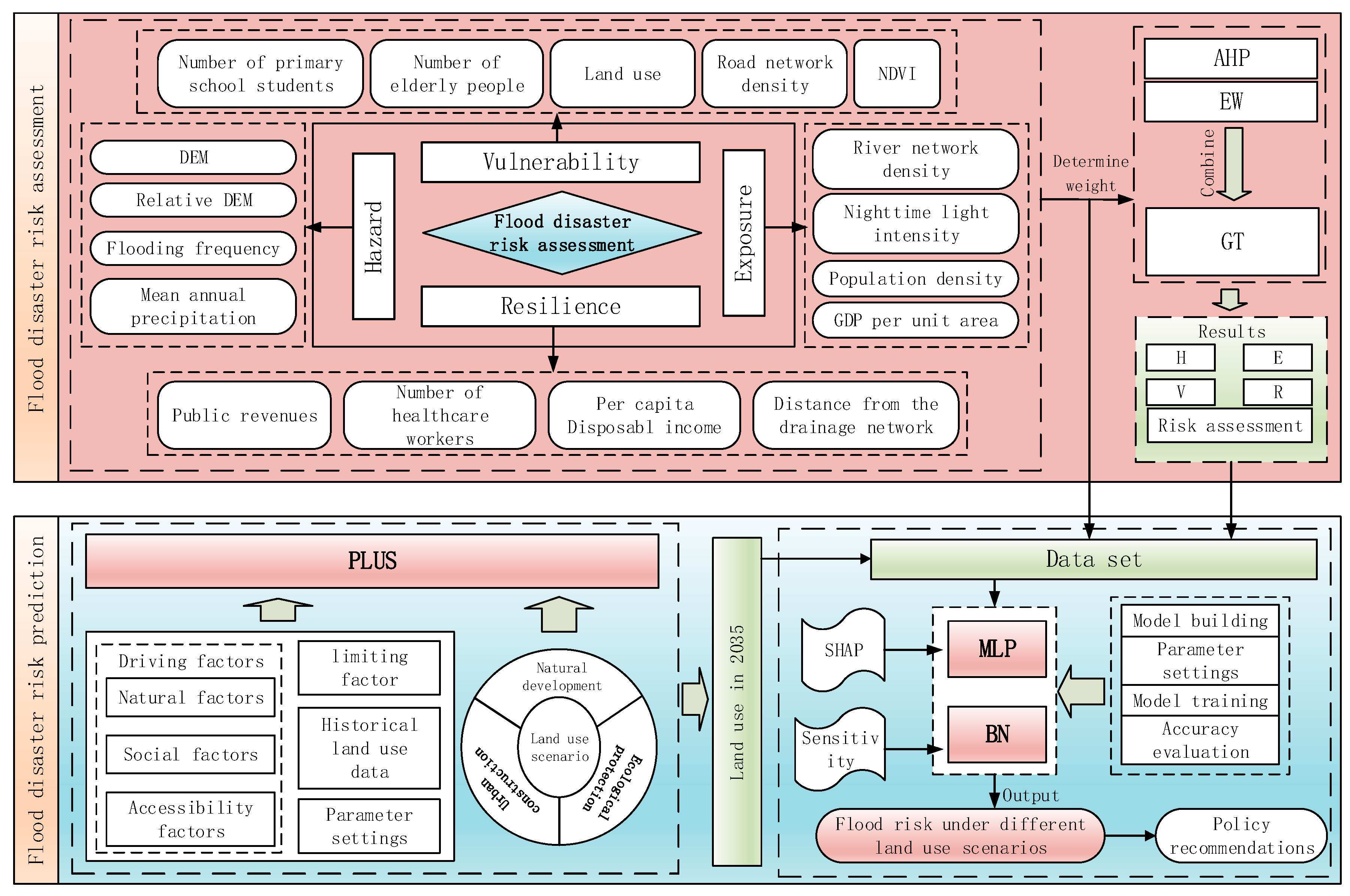
In this study, we assess flood risk in the CZT urban agglomeration using a framework that integrates hazard, exposure, vulnerability, and resilience. We further evaluate future flood risk under different land use scenarios by simulating land use changes and training MLP and BN models (Figure 2).

3.1. Flood Risk Assessment

3.1.1. Flood Risk Assessment Framework

This chapter applies the disaster risk system theory, utilizing the Hazard–Exposure–Vulnerability–Resilience (H-E-V-R) framework to assess flood risk in the CZT urban agglomeration. Within this framework, hazard refers to the intensity of the disaster-triggering factor, exposure denotes the extent of the disaster-prone environment, vulnerability reflects the susceptibility of the affected elements, and resilience represents the capacity to recover post-disaster [42]. Thus, flood risk in the CZT urban agglomeration can be quantified as the ratio of the product of H, E, and V to R. The formulas for calculating the indices in the framework are as follows:
R i s k = H × E × V R
H = i = 1 a W i × X i
E = i = 1 b W i × X i
V = i = 1 c W i × X i
R = i = 1 d W i × X i
where Risk represents flood risk, H represents flood hazard, E represents flood exposure, V represents flood vulnerability, R represents flood resilience, Wi is the weight of the indicator, and Xi is the standardized indicator.
Indicators are standardized using the Min–Max method with the following formula:
X i = a i a min a max a min
X i = a max a i a max a min
where a i and X i represent the original and standardized values of the indicator, respectively, and a max , a min represent the maximal and minimal values of the indicator, respectively. Positive indicators are normalized using Equation (6), and negative indicators are normalized using Equation (7).

3.1.2. Construction of a Risk Indicator System for Flood Risk

Select four indicators for hazard assessment. Flood frequency, which reflects a region’s historical flood susceptibility, was derived by analyzing remote sensing images of the CZT urban agglomeration during the May–June flood seasons from 2014 to 2023, combined with historical rainfall data to distinguish temporary inundation from permanent water bodies. Multi-year average annual rainfall, an indicator of precipitation intensity and persistence, was calculated using 40 years (1984–2023) of global meteorological station data, interpolated in ArcGIS to produce a long-term precipitation raster. Topographic influences were assessed through absolute elevation (from DEM data) and relative elevation, the latter computed as the standard deviation of elevation within a 5 × 5 raster neighborhood using ArcGIS’s focal statistics, capturing local terrain variability and its role in flood risk.
Flood exposure refers to the extent to which a region’s population, economic assets, resources, and environment may be affected by flooding. This study selects four exposure indicators. River network density reflects the concentration of waterways in a region; during extreme rainfall events, higher river density leads to increased runoff volume, faster water flow, and greater risks of dike breaches and overflow, particularly affecting areas along rivers and downstream. The river network density for the CZT urban agglomeration was extracted using DEM data processed in ArcGIS through hydrologic correction (fill sinks), flow direction analysis, flow accumulation analysis, stream reclassification, and stream ordering. The other three indicators—population density, nighttime light intensity, and gross product per unit area—represent the intensity of human activity. Regions with higher population density, stronger economic concentration (reflected by nighttime lights), and greater GDP per unit area typically experience more severe impacts when floods occur.
Flood risk-bearing vulnerability refers to the potential damage a specific region or system may sustain when exposed to flooding. In this study, we assess flood risk vulnerability using five key indicators. Land use and NDVI represent environmental vulnerability—regions with higher built-up land cover and lower vegetation density exhibit greater susceptibility to flood impacts. Elementary school children and the elderly reflect social vulnerability, as these groups are particularly susceptible during disasters due to limited mobility and higher dependency. Road network density serves as an indicator of transportation and emergency response vulnerability. Disruptions in transportation infrastructure can lead to paralyzed mobility and delayed relief efforts, exacerbating disaster consequences.
Flood disaster resilience is strongly influenced by three key factors. Funding determines both governmental relief efforts and individual self-help capabilities. Adequate financial resources enable timely emergency responses, recovery programs, and long-term mitigation strategies [43]. Regions with stronger healthcare systems can better minimize casualties by providing urgent care and managing post-disaster health crises [44]. Drainage infrastructure directly affects the magnitude and duration of flood impacts. Efficient drainage systems reduce surface water accumulation, accelerating recovery and mitigating long-term damage.

3.1.3. Multicollinearity Test

The presence of high intercorrelations among predictor variables may induce multicollinearity, potentially biasing model parameter estimates. To assess this phenomenon quantitatively, we employ the variance inflation factor (VIF) as a diagnostic measure for multicollinearity detection [45]. Following conventional statistical practice, predictor variables exhibiting VIF values exceeding the threshold of 10 were identified as demonstrating significant multicollinearity and consequently removed from subsequent analyses [46]. This paper uses Python to calculate the VIF results as shown in Table 2.
As shown in Table 2, the VIF values for all indicators are less than 10, indicating no significant multicollinearity among the indicators, making them suitable for use in subsequent experiments.

3.1.4. Determination of Indicator Weights

Relying solely on a single weight determination method often leads to results that are either excessively subjective or overly objective. To address this issue, this paper employs the Analytic Hierarchy Process (AHP) to determine the subjective weights of the indicators and the entropy weight method (EW) to derive their objective weights. These two approaches are then integrated using game theory (GT) to obtain a more balanced and realistic set of weights. The final weight results are presented in Table 3.
Game theory treats different weight assignment methods (e.g., AHP and entropy weight method) as “players” in a game, where negotiation or competition yields a consensus, with the final weights representing an equilibrium solution. To operationalize this, a linear combination of the two methods’ weight vectors is constructed (Equation (8)), followed by optimization of the combination coefficients (Equations (9) and (10)) using game-theoretic distance minimization. The final weights are derived from Equation (11) and presented in Table 3, where + denotes a positive role, − denotes a negative role, and / representatives have different roles at the normative level based on categorization.
W = μ 1 w z T + μ 2 w k T
min | | W w | | 2
w z w z T w z w k T w k w z T w k w k T u 1 u 2 w z w z T w k w k T
W = μ 1 μ 1 + μ 2 w z T + μ 2 μ 1 + μ 2 w k T
where W is the game theory weight, μ 1 and μ 2 are the linear combination coefficients, u 1 and u 2 are the optimal combination weights, and w z and w k are the weights of hierarchical analysis and entropy weighting.

3.2. Land Use Simulation

The PLUS model is an enhanced patch-level land use simulation framework that builds upon traditional cellular automata (CA) approaches. This advanced model incorporates two core components: (1) a Land Expansion Analysis Module (LEAS) powered by Random Forest algorithms for land use change analysis, and (2) a Cellular Automata Module (CARS) featuring Random Seed Generation to simulate spatial dynamics. By integrating these modules, the PLUS model achieves more accurate and realistic simulations of land use patterns at the patch level compared to conventional CA models [47].
This study employs the PLUS model to simulate land use patterns in the CZT urban agglomeration for 2035 under various scenarios, enabling flood risk prediction under different land use configurations. The simulation process utilized land use change data from 2017 to 2023 to generate a confusion matrix, which served as the original matrix for Markov chain quantity prediction. Recognizing land use as a complex system influenced by multiple factors [48], we selected 15 driving factors across three key dimensions: (1) natural environment (elevation, slope, NDVI, mean annual precipitation and temperature mean annual temperature, and precipitation); (2) socioeconomic factors (population density, GDP per unit area, and nighttime light intensity); and (3) accessibility (distance from first-class, second-class, and third-class roads, distance from the district/county center, distance from highway, distance from the railway).
Using 2017 as the baseline year, we simulated the 2023 land use layout and validated it against actual 2023 data. The model achieved a Kappa coefficient of 0.78 and an overall accuracy of 0.87, meeting the required precision thresholds. These validated parameters were subsequently applied to simulate the 2035 land use scenarios for the CZT urban agglomeration.
Different land use scenarios significantly influence flood risk. To assess these impacts, this paper establishes three distinct scenarios—natural development, urban construction, and ecological protection—leveraging the PLUS model’s flexible parameter-setting capabilities to simulate land use layouts under each scenario.
Natural Development Scenario: This scenario adheres to the historical land use evolution trends observed from 2017 to 2023, determining transition probabilities for each land use category without artificial interventions.
Urban Construction Scenario: Aimed at fostering economic growth and urban expansion, this scenario increases the transition probabilities of cultivated land, forest, and grassland to construction land by 20%, while decreasing the conversion probabilities of construction land to cultivated land, forest, grassland, and water by 25%. This is consistent with previous research [49,50] and the “Development Plan for Changsha Zhuzhou Xiangtan Urban Agglomeration.”
Ecological Protection Scenario: The “Land use planning of Changsha Zhuzhou Xiangtan Urban Agglomeration (2021–2035)” states that the region’s “ecological green heart” must be protected. So, this scenario reduces the transition probabilities of forest, grassland, and water to construction land by 50%, decreases the conversion of cultivated land to construction land by 30%, and increases the transition probabilities of cultivated land and grassland to forest by 20%.

3.3. Probabilistic Flood Risk Prediction

3.3.1. Multilayer Perceptron

➀ Model Principle
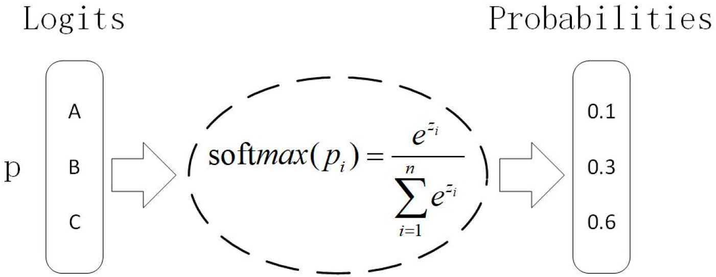
MLP is a feed-forward neural network model that extends the basic perceptron by incorporating multiple single-layer perceptrons. Its architecture follows a hierarchical “input layer-hidden layer-output layer” structure (Figure 3), where each hidden layer contains numerous neuron nodes. These nodes apply nonlinear activation functions—such as ReLU, Sigmoid, or Tanh—to transform input features, enabling the model to approximate complex nonlinear relationships. By stacking multiple hidden layers, the MLP progressively extracts higher-level features from raw data, overcoming the limitations of a single-layer perceptron in handling nonlinear, differentiable problems.
In an L-layer network, input layers receive N-dimensional vectors transformed by activation function f ( * ) . Common activation functions include Sigmoid, Tanh, and ReLU. Parameters w l and b l denote weights and biases connecting layer l to layer l + 1 . Variable P l represents input to layer l , while O l corresponds to output from layer l .
P l = O l 1 × W l + b l
O l = f ( P l )
➁ SHAP Interpretability Analysis
SHAP interpretability analysis is a game-theoretic approach for explaining machine learning models. It quantifies feature importance by evaluating each feature’s marginal contribution to model predictions. The SHAP value calculation involves two key steps: (1) assessing the prediction difference when a feature is included versus excluded to determine its individual impact, and (2) comprehensively evaluating the feature’s contribution across all possible feature combinations, with the final Shapley value computed as a weighted average (Equation (14)). In this study, we employ SHAP summary plots to visualize the contribution of flood risk factors (e.g., land use patterns) to model outputs, thereby enhancing model interpretability and providing actionable insights into flood risk drivers.
μ i = S N i | S | ! ( M | S | 1 ) ! M ! f x ( S i ) f x ( S )
In Equation (14), μ i represents the contribution of the feature i to the model output, N i is the set of features, M is the total number of features in the sample, f x ( S i ) refers to the predicted value of the model when the sample has only feature values in S i , and f x ( S ) is the predicted value of the model when the sample has only feature values in S .

3.3.2. Bayesian Network

➀ Model Principle
The BN framework comprises two core components: a directed acyclic graph (DAG) and a conditional probability table (CPT). As a probabilistic graphical model, BN’s key advantage lies in its ability to simulate human cognitive processes for causal reasoning, particularly in decision-making under uncertainty [51]. Leveraging its probabilistic reasoning mechanism and causal modeling capabilities, BN has shown exceptional utility in uncertainty reasoning and has emerged as a fundamental analytical tool for complex decision-making scenarios. The BN model supports bidirectional inference: (1) predicting target node probabilities using prior knowledge, and (2) deriving posterior probabilities for root nodes based on observed target node states and the network structure [52]. The model’s mathematical foundation is expressed as follows:
P ( A | B ) = P ( A B ) P ( B ) = P ( B | A ) P ( A ) P ( B )
In Equation (6), P ( A | B ) is the posterior probability, P ( A B ) is the probability that A and B occur together, P ( A ) and P ( B ) are the probabilities that A and B occur, also called the prior probabilities, and P ( B | A ) is the conditional probability.
➁ Sensitivity analysis
Kjaerulff et al. [53] introduced a sensitivity analysis method for BN using GENIE software, which systematically evaluates the influence of parent nodes on target nodes. When a parent node demonstrates weak sensitivity to a target node, changes in the parent node’s state will have minimal impact on the target node’s probability distribution. Conversely, highly sensitive parent nodes exert substantial influence on target node outcomes. This sensitivity analysis provides crucial insights for network refinement and validation, particularly in identifying key drivers within complex probabilistic systems [53].

3.3.3. Model Dataset and Model Construction

➀ Model datasets
This paper employs flood risk evaluation results and their criterion layer and indicator layers as data sources to calculate flood risk probabilities through a multi-step analytical process. First, 50,000 random points are generated across the study area, with input layer attributes superimposed onto these points to create an initial dataset for both MLP and BN models. The land use probabilities are then adjusted based on scenario-specific projections derived from the PLUS model, allowing the updated MLP and BN models to assess the impacts of different land use configurations on future flood risk. To ensure consistency between models, the continuous MLP outputs are classified into discrete risk probability levels—aligned with the BN’s native probabilistic outputs—using a hybrid approach that combines the natural breaks (Jenks) method with expert validation, with detailed classification thresholds provided in Table 4.
➁ model construction
This study employs an MLP implemented in Python to predict future flood risks under varying scenarios. The network architecture comprises three layers: an input layer with 17 neurons for feature processing, a hidden layer with 15 neurons using the Tanh activation function to model nonlinear relationships, and an output layer with 4 neurons activated by softmax for probabilistic classification (Figure 4). The architecture’s input and output layer dimensions correspond to the predictor variables (n = 17) and four risk classification categories, respectively. The hidden layer configuration was optimized through Bayesian optimization, with hyperparameter selection guided by maximizing ten-fold cross-validation accuracy. The Adam optimizer trains the model by minimizing categorical cross-entropy loss, with the softmax function transforming final outputs into a probability distribution across four flood risk categories: low, moderate, high, and serious.
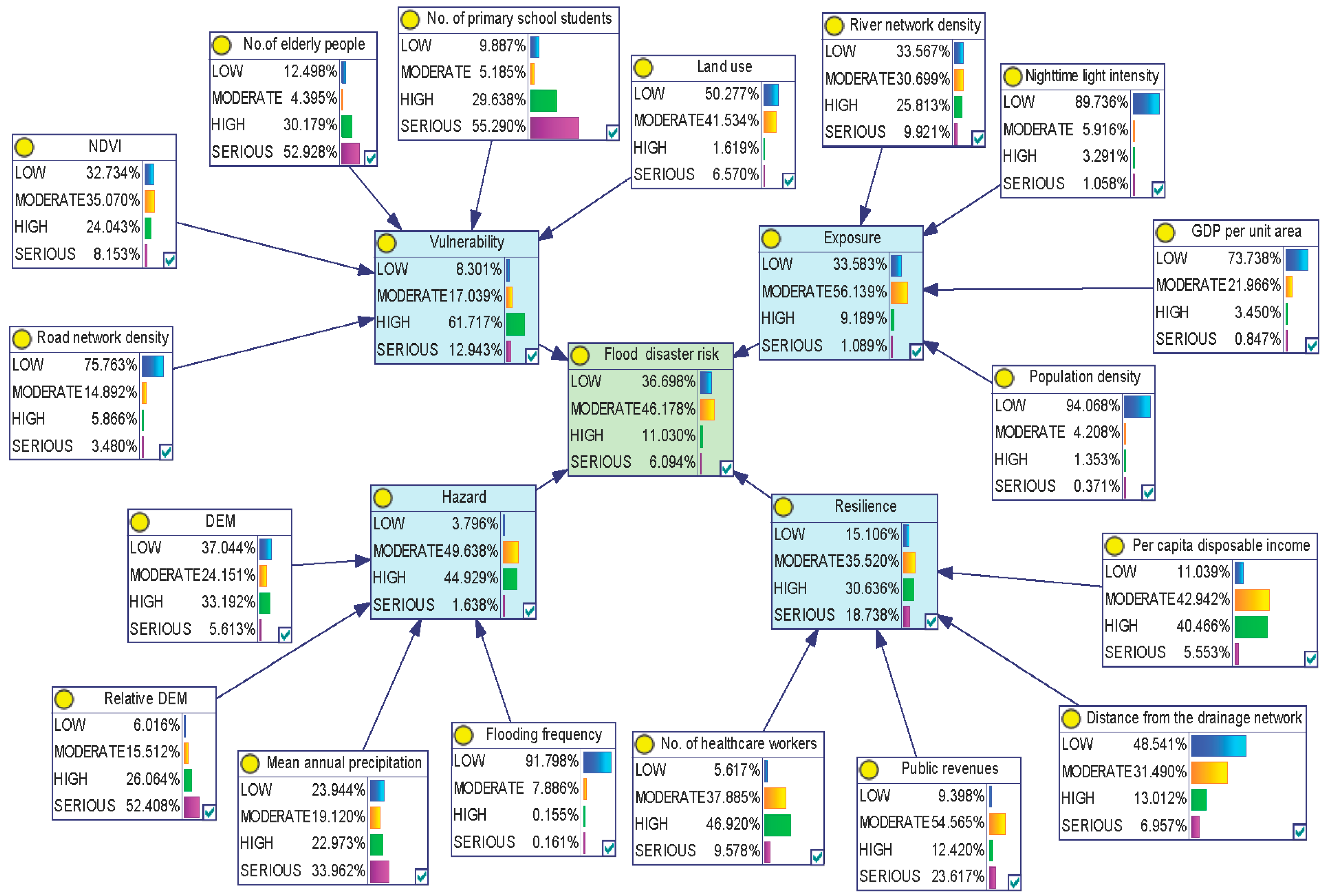
This study develops a BN model using GENIE software integrated with Python to assess flood risk probabilities in the CZT urban agglomeration. The network structure organizes flood risk factors hierarchically: individual indices serve as parent nodes, synthesized criterion layers function as intermediate nodes, and flood risk classification acts as the target node. Through parameter learning methods, we train the model using sample data statistics to derive conditional probability relationships, with the final network structure and probabilities presented in Figure 5.

3.3.4. Flood Risk Index

To facilitate quantitative comparison of flood risk across different land use scenarios, this study introduces a comprehensive flood risk index (FRI). This index was selected through a comprehensive process involving sensitivity analysis of the weights assigned to different groups (all of which are equidistant) and expert experience. It integrates probabilistic risk assessments by weighting each risk category (low, medium, high, and serious) with corresponding severity scores of 25, 50, 75, and 100, respectively. The FRI is calculated as a weighted sum of risk probabilities, with a mathematical expression in Equation (16).
F R I = L × 25 + M × 50 + H × 75 + S × 100
In Equation (16), L , M , H , and S represent the probabilities of low risk, moderate risk, high risk, and serious risk, respectively.

4. Results

4.1. Flood Risk Assessment

4.1.1. Hazard Assessment

Using the raster calculator, the four hazard indicators were weighted and stacked in a raster according to Equation (2). Subsequently, the resultant raster was classified into five distinct risk classes: low hazard, medium-low hazard, medium hazard, medium-high hazard, and high hazard, as depicted in Figure 6.
Based on the results of the flood hazard assessment and its corresponding indicator grid, it can be observed that high hazard areas are distributed along both sides of the Xiang River and in the eastern valley. Along the Xiang River, the banks are exposed to the risk of inundation throughout the year, with a high frequency of flooding events. This persistent threat of inundation contributes significantly to the high flood hazard in these areas. In the eastern valley, the absolute elevation is low, and the relative elevation is also low. This indicates that the terrain in this region is flatter compared to its surrounding areas, and there is a substantial difference in elevation between the valley and the adjacent regions. As a result, water tends to accumulate in the valley, increasing the likelihood of flooding and thus leading to a high hazard level.

4.1.2. Exposure Assessment

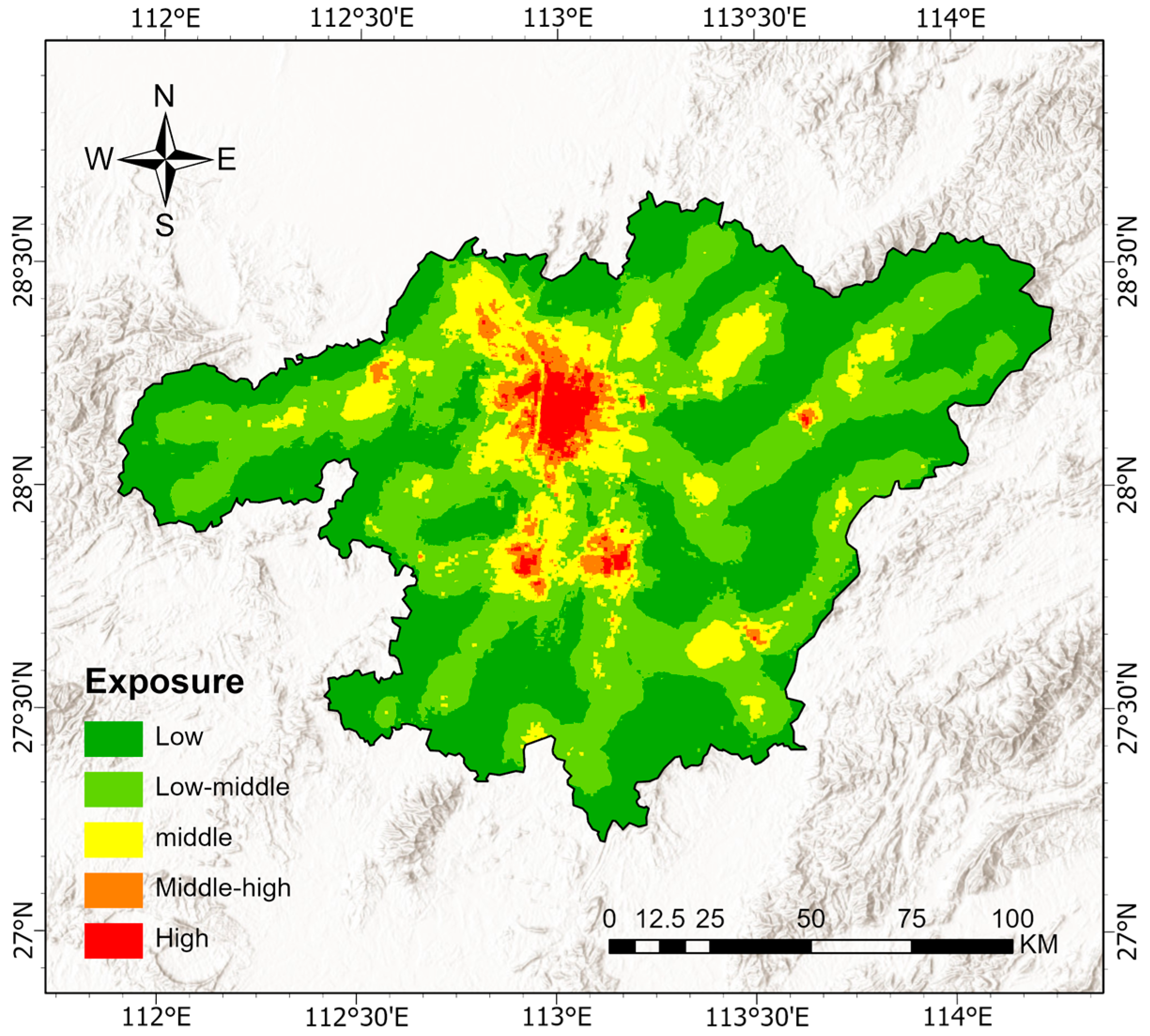
Employing the raster calculator, the four exposure indicators were weighted and superimposed onto the raster according to Equation (3). Subsequently, these were classified into five categories, as presented in Figure 7.
In terms of flood exposure, it is predominantly concentrated around the main urban areas of the three major cities in the CZT urban agglomeration. These areas are clustered along the banks of the Xiang River, and the exposure level decreases radially outward from this core. Specifically, high-exposure areas are situated in the central part of the CZT urban agglomeration. High-exposure areas represent high-value zones, characterized by dense population, elevated output per unit area, and a high nighttime lighting index, making them the core hubs of urban development. In contrast, medium-exposure areas function as urban–rural transitional zones, exhibiting relatively moderate development levels.

4.1.3. Vulnerability Assessment

The five vulnerability indicators were integrated using the raster calculator (Figure 8), weighted and superimposed according to Equation (4), and classified into five distinct levels.
High flood vulnerability areas are predominantly concentrated in the northern part of the study area, while medium-high-vulnerability zones are primarily distributed in the northwest and southeast. High-vulnerability areas exhibit a dense road network and are predominantly characterized by arable and construction land. Intensive economic development in these zones has led to significant population concentration, including a higher proportion of elderly residents and elementary school students. Rapid urbanization has also encroached upon green spaces, resulting in low vegetation coverage. Consequently, these areas face inadequate drainage capacity during flood events, hindered emergency evacuation, and diminished natural water retention, collectively exacerbating disaster risk.

4.1.4. Resilience Assessment

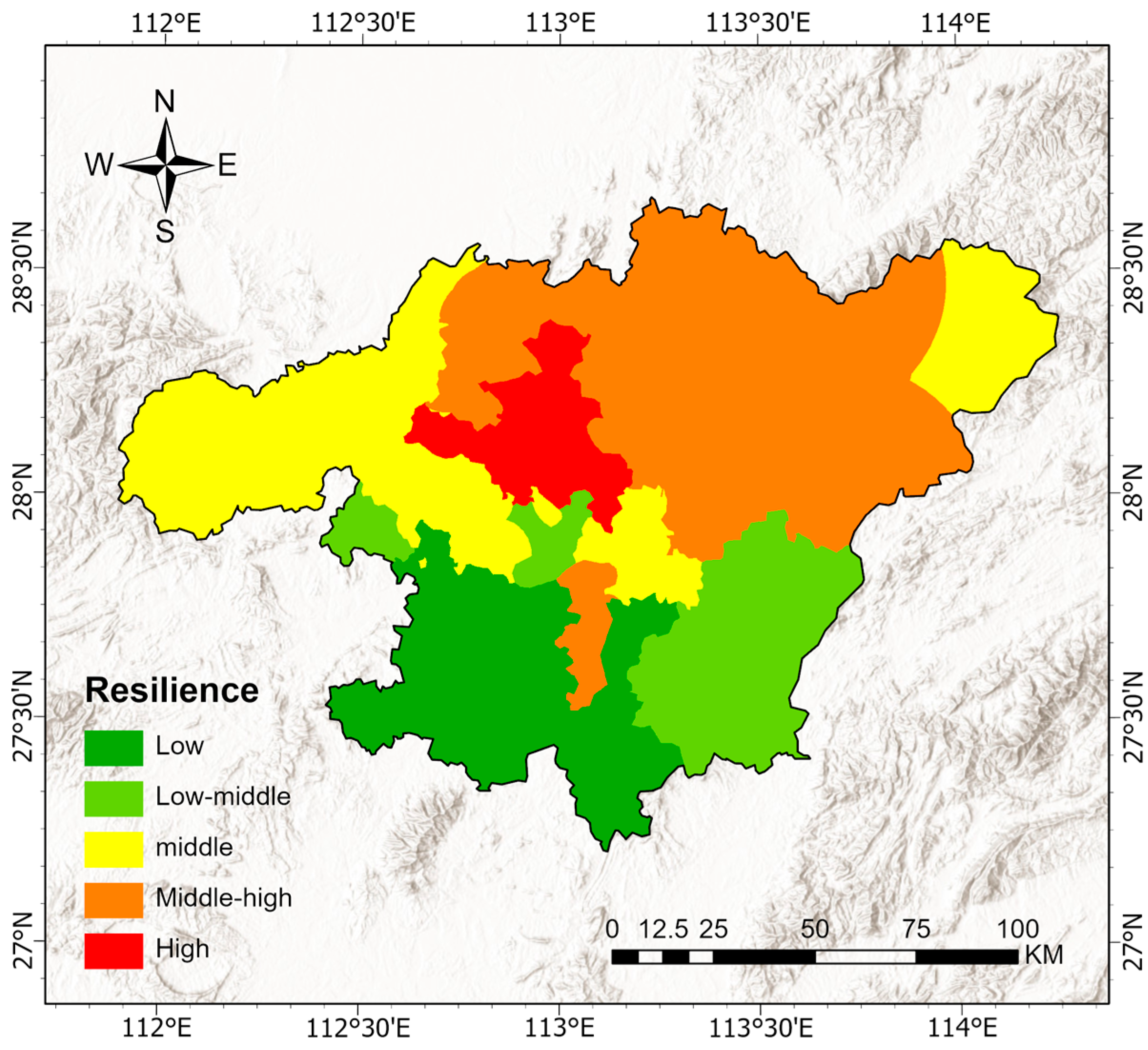
The four resilience indicators were weighted and integrated through raster calculation (Equation (5)), then classified into five distinct tiers, as illustrated in Figure 9.
Areas of high resilience are dispersed throughout the region, with notable clustering in the central zone. High-resilience regions are characterized by strong public fiscal revenue, enabling robust financial support for post-disaster recovery. These areas also benefit from a greater concentration of healthcare professionals, ensuring effective medical response and public health protection following disasters. Additionally, higher per capita disposable income enhances residents’ intrinsic capacity for recovery. From an infrastructure perspective, these regions maintain optimal drainage network density, resulting in superior floodwater management capabilities during extreme weather events.

4.1.5. Flood Risk Assessment

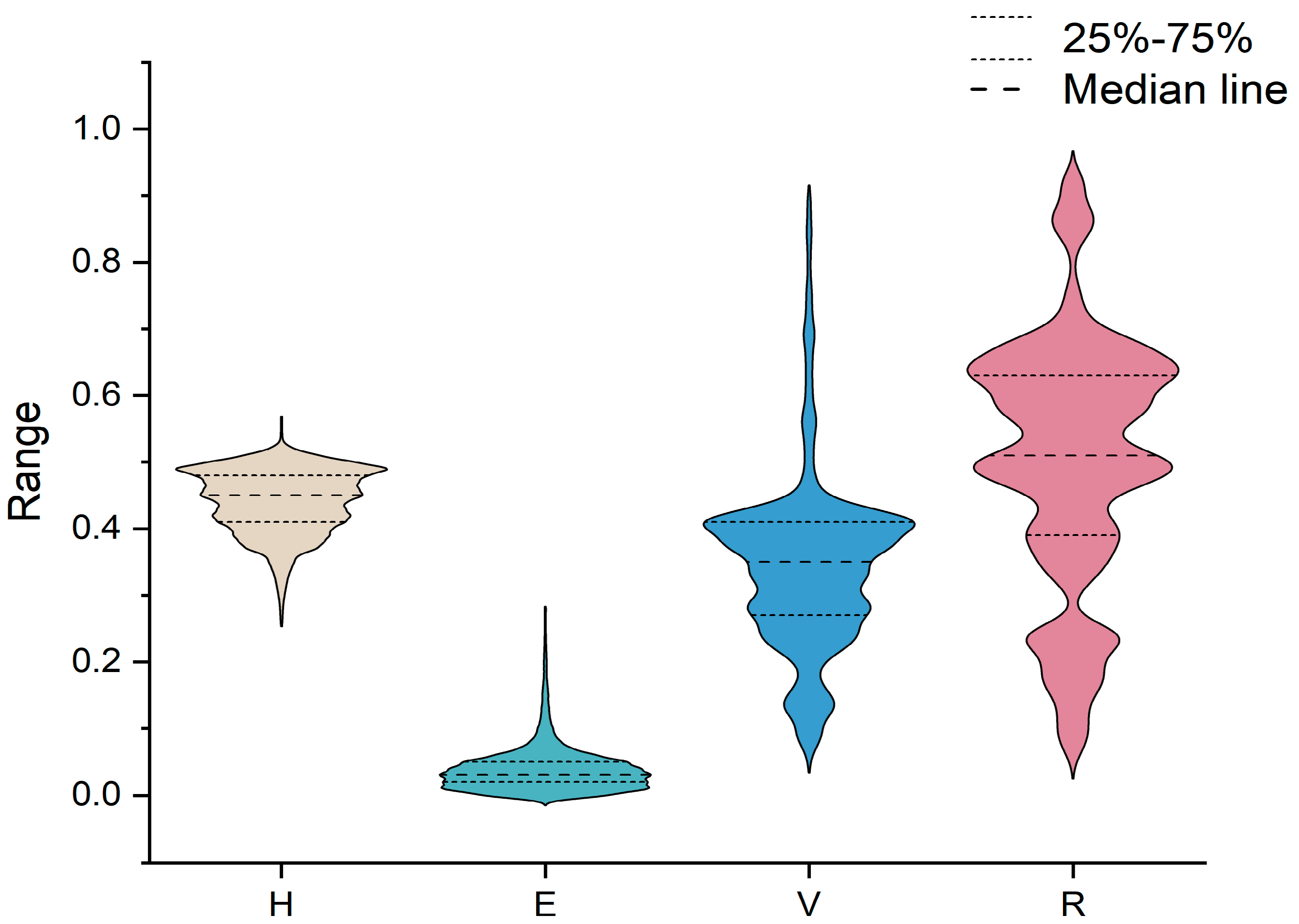
The weighted distributions of hazard, exposure, vulnerability, and resilience indicators are presented in Figure 10. Hazard levels predominantly fall within the 0.4–0.5 range, with minimal variation between high and low values, indicating uniformly medium-high hazard conditions where even the highest values are only relatively elevated. Similarly, exposure values show limited variability but are mostly concentrated below 0.15, suggesting generally low exposure risk across the study area. In contrast, vulnerability exhibits greater variation, with a median slightly exceeding 0.3. Resilience also demonstrates significant dispersion, with a median of approximately 0.5. These pronounced differences in vulnerability and resilience are more likely to drive regional disparities in flood risk.
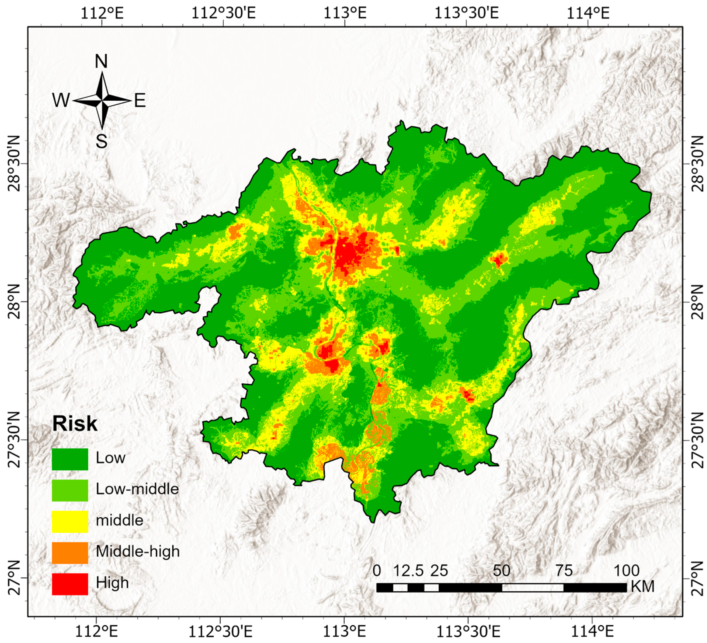
Using the raster calculator, the hazard, exposure, vulnerability, and resilience layers were weighted and integrated according to Equation (1), then classified into five distinct risk categories (Figure 11).
High-flood-risk areas are predominantly clustered in the central study area, forming contiguous blocks along both sides of the Xiang River. Medium-high- and medium-risk areas radiate outward from high-risk zones in a gradient-decreasing pattern, while low-risk areas are primarily scattered in remote mountainous regions with limited socioeconomic activity. Areas with high flood risk are characterized by low elevation, minimal relative relief, and flat topography, rendering them susceptible to waterlogging and elevated flood hazards. These regions face compounded risks due to (1) high population and economic density, where urban expansion has increased impervious surfaces, reduced groundwater infiltration capacity, and diminished vegetation cover—collectively exacerbating flood exposure and vulnerability; and (2) limited effectiveness of existing financial and healthcare resources (despite being comparatively higher than surrounding areas) in mitigating flood impacts. Nevertheless, in peripheral zones adjacent to high-risk areas, while hazard intensity, exposure, and vulnerability remain elevated, the enhanced recovery capacity significantly mitigates overall flood risk. This finding highlights the critical need for comprehensive flood risk management strategies that address both natural and socioeconomic dimensions. Future mitigation efforts should therefore adopt a dual approach: (1) improving natural landscape features (e.g., through green infrastructure and water retention systems), coupled with (2) strengthening institutional preparedness via optimized emergency response protocols, robust flood protection infrastructure, and upgraded regional healthcare systems.

4.2. Land Use Simulation

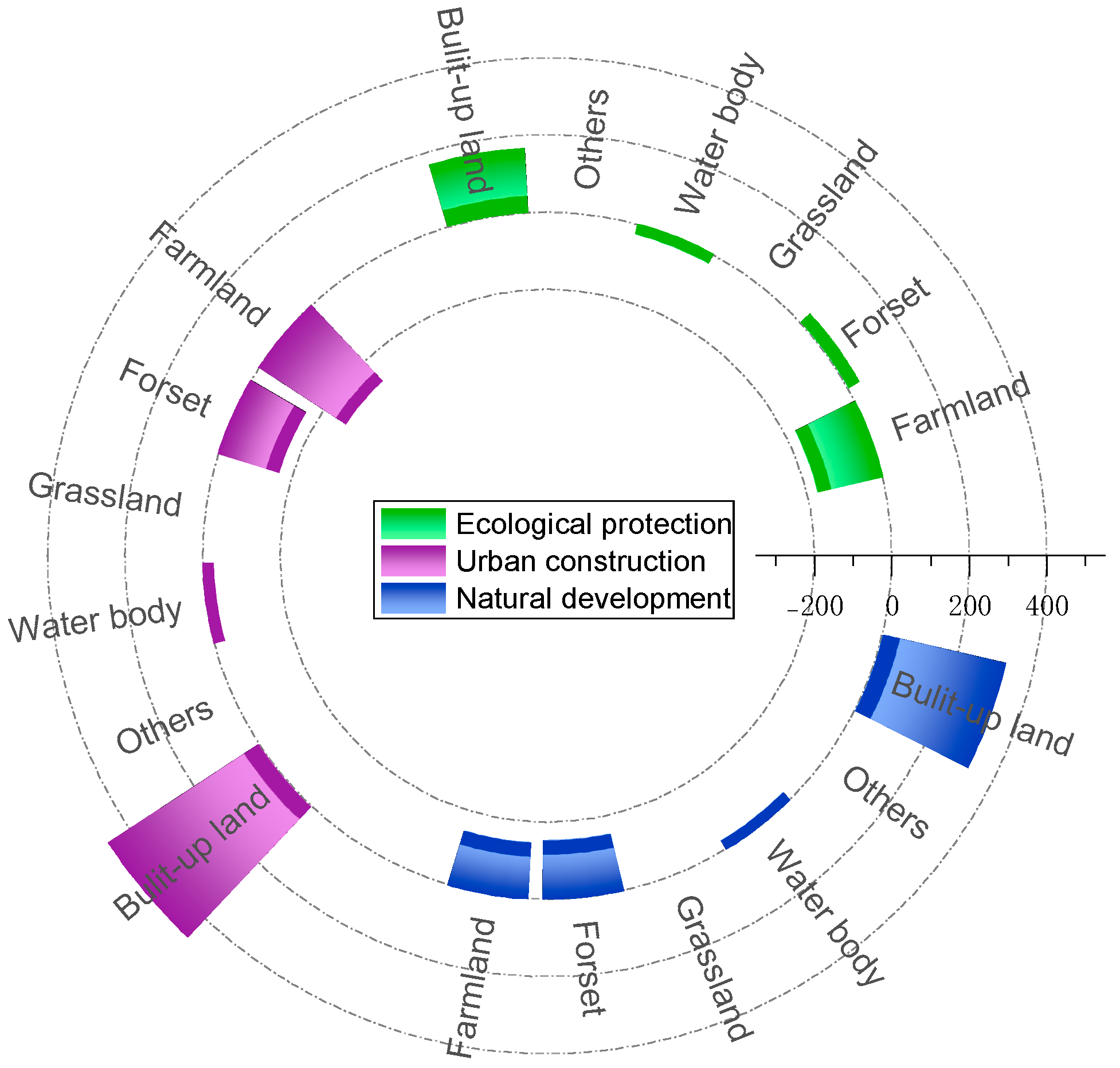
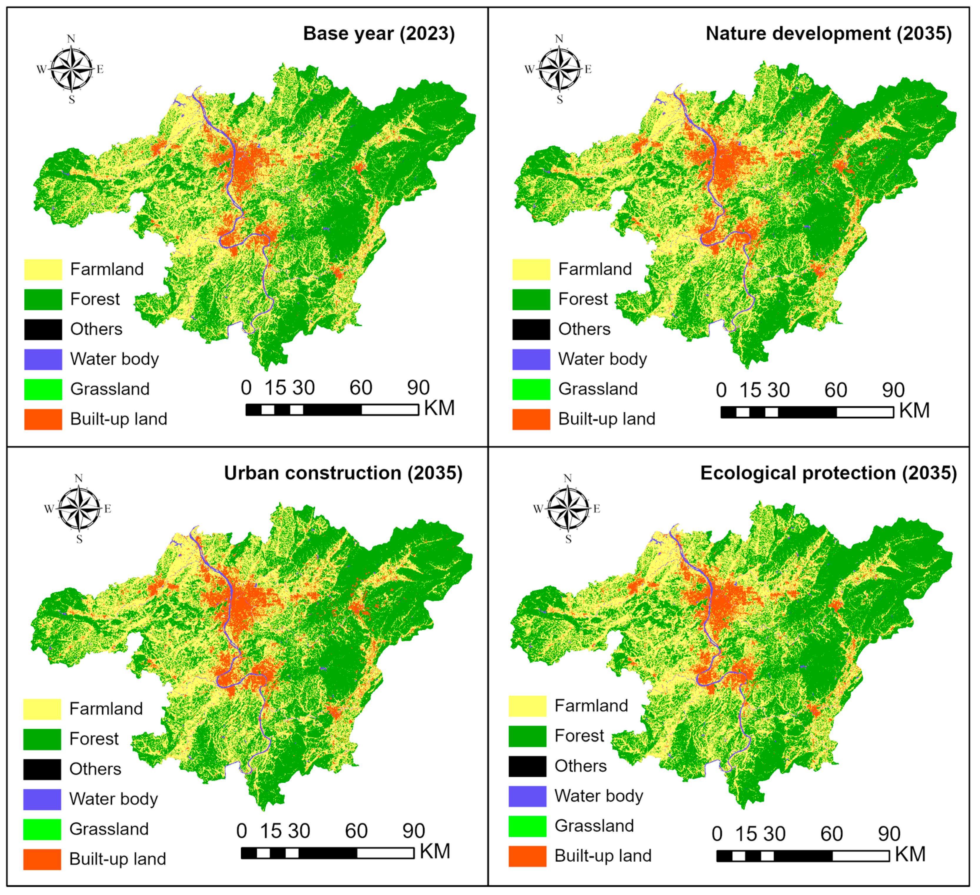
We employed Markov chain analysis to project land use changes under multiple scenarios, calculating transition probabilities between land use types to generate quantitative forecasts (Figure 12). These probability matrices, combined with neighborhood weight parameters and conversion rules, were subsequently integrated into the CARS module of the PLUS model. This implementation yielded spatially explicit land use projections for the year 2035 across all considered scenarios, as visualized in Figure 13.
A comparison of the natural development scenario with the 2023 baseline reveals substantial land use changes. The analysis shows a dramatic expansion of built-up land, increasing by 326.3 square kilometers, alongside a minor growth in other land from 0.21 to 0.27 square kilometers. In contrast, all other land categories experienced declines, with forest showing the most significant reduction of 153.07 square kilometers. Additional decreases occurred in farmland, which diminished by 146.37 square kilometers, water bodies, which reduced by 26.88 square kilometers, and grassland, which saw a slight decrease of 0.03 square kilometers.
The town development scenario significantly alters the probability of land use conversion. Compared to both the 2023 baseline and the natural development scenario, this scenario results in a substantially larger expansion of built-up land, alongside more pronounced reductions in cropland and forest land. Specifically, the areas of cultivated land, forest land, grassland, water bodies, unused land, and construction land are 7309.50 km2, 9335.87 km2, 1.52 km2, 290.25 km2, 0.27 km2, and 1665.02 km2, respectively. These figures represent increases of 3.4%, 1.7%, 2.9%, 9.3%, and 25.3% compared to 2023 levels. Spatially, urban expansion has intensified to support economic growth, with construction land extending outward and becoming more densely consolidated in areas previously characterized by mixed land use. Notably, cultivated land adjacent to construction zones has experienced significant encroachment.
The ecological conservation scenario generally enhances the retention of forest land and increases the likelihood of other land use types being converted into forest land. Compared to the base period, forest land area rises from 9501.61 km2 to 9534.45 km2. While arable land decreases relative to the natural development scenario, it experiences a significant increase compared to the urban development scenario. Due to the prioritization of ecological protection and controlled economic land development, construction land expansion is suppressed. Its area shows only a marginal increase from 2023, with a notably smaller growth rate than under the other two scenarios. Spatially, construction land expansion is largely confined to peripheral areas, with minimal encroachment on forest and cultivated land distant from urban centers. Additionally, under the constraints of the ecological protection scenario, some cultivated land adjacent to forested areas is converted into forest land, further contributing to ecological conservation.

4.3. Probabilistic Flood Risk Prediction

4.3.1. MLP-Based Probabilistic Prediction of Flood Risk

The MLP learns from the training data to develop a predictive model for estimating future flood risk probabilities. In this study, a ten-fold cross-validation approach is employed to evaluate model performance. The dataset is partitioned into ten subsets, and the model’s overall accuracy is assessed by computing the average prediction error rate across all subsets. The resulting error rates from the ten-fold cross-validation are presented in Table 5.
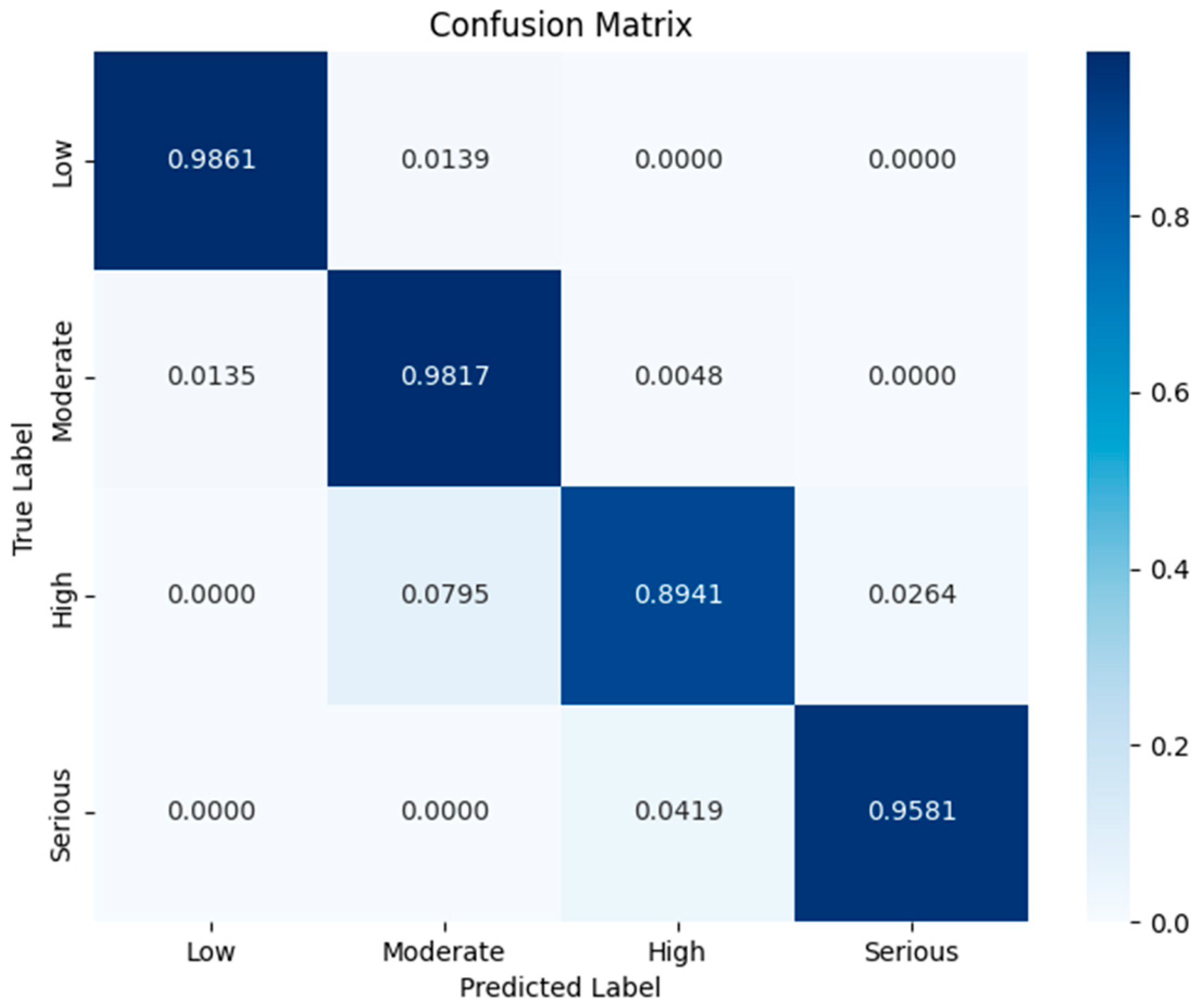
The ten-fold cross-validation results demonstrate strong predictive performance for the MLP model, with an average error rate of 2.17% and an accuracy rate of 97.83%. This high level of accuracy supports the model’s reliability in predicting future flood risks under varying land use scenarios. To further evaluate model performance, we plotted the accuracy and loss curves for both the training and test sets, as well as a confusion matrix to assess per-class prediction accuracy (Figure 14 and Figure 15).
As shown in Figure 14, both the training and test set accuracy curves exhibit steady, synchronous increases before stabilizing, while the loss curves demonstrate a corresponding synchronous decline before plateauing. The test set curves show minimal fluctuations, indicating stable learning. The final training accuracy is marginally higher than that of the test set, while the test loss is slightly greater than the training loss—a pattern consistent with well-generalized models that exhibit neither over-fitting nor under-fitting. Figure 15 further illustrates the model’s performance across risk categories, with prediction accuracies of 0.9861 (low risk), 0.9817 (moderate risk), 0.8941 (high risk), and 0.9581 (very high risk). While the high-risk category (0.8941) falls slightly below 0.90, all other categories achieve strong predictive performance.
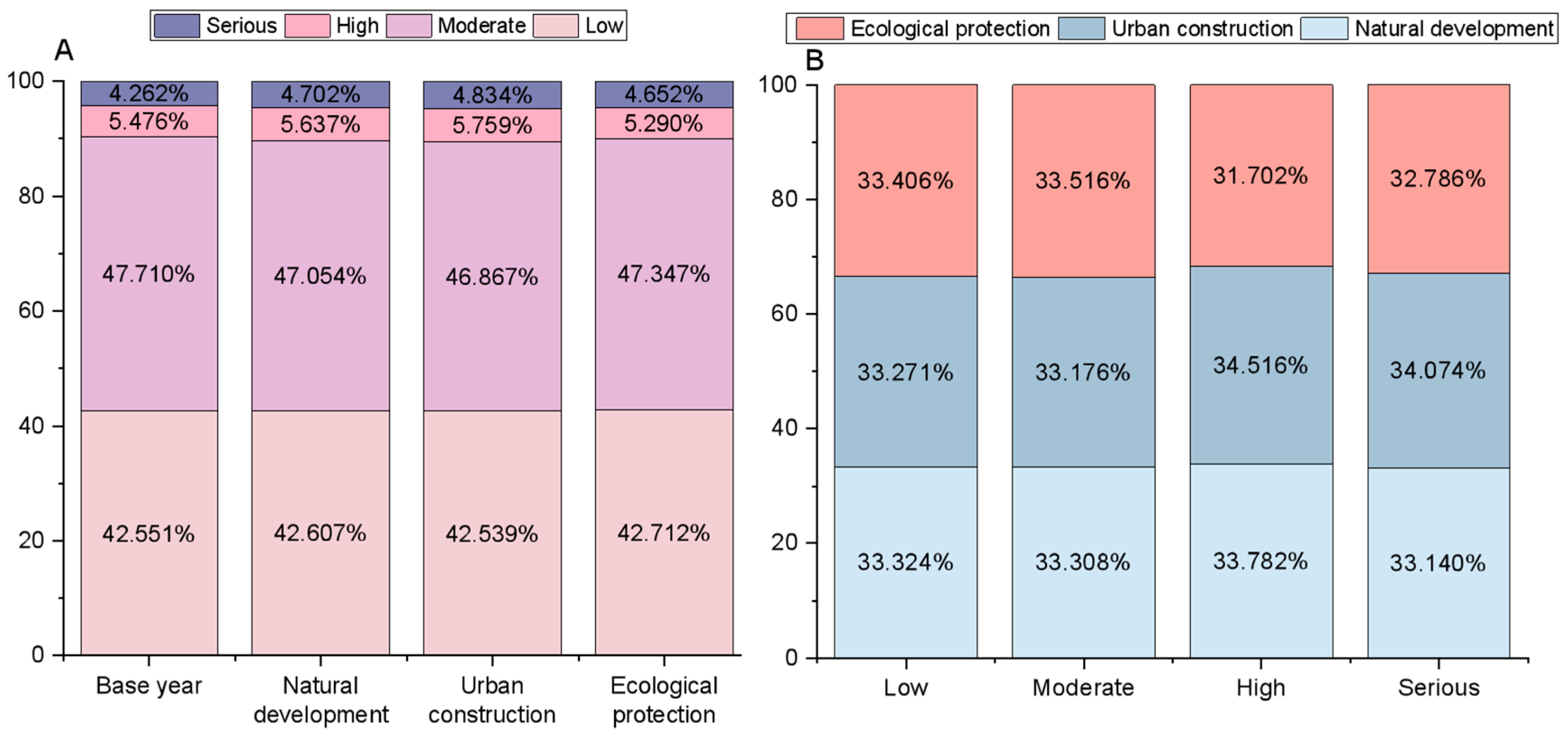
By adjusting the land use probabilities in the trained MLP model, we obtained the flood risk probabilities for different land use scenarios, as illustrated in Figure 16. Notably, the risk assessment process employs five classification levels to provide more detailed risk characterization, whereas the prediction process uses four levels to optimize model accuracy. This distinction arises because while a greater number of classification levels within a certain range enhances the granularity of risk assessment results, a reduced number of categories improves the predictive performance of the model.
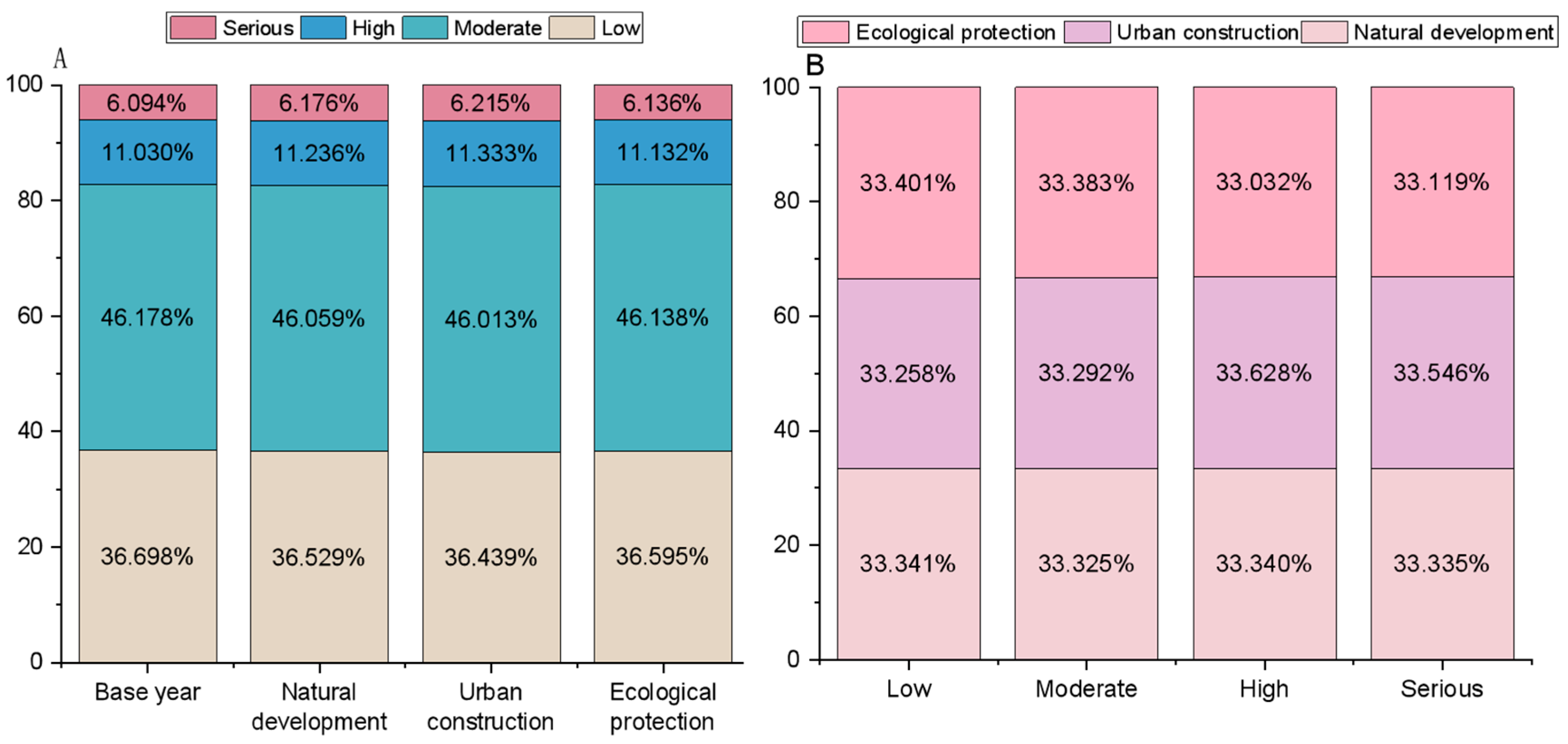
Figure 16A demonstrates that all three scenarios project higher proportions of serious and high flood risk compared to the base year. The urban construction scenario exhibits the most severe risk profile, with serious risk reaching 4.834%—the highest among all scenarios. Comparative analysis reveals that the ecological protection scenario presents the most favorable risk distribution, characterized by the lowest proportions of serious (4.652%) and high risk (5.290%), alongside the highest proportions of moderate (47.347%) and low risk (42.712%). The natural development scenario shows intermediate values, while the urban construction scenario consistently demonstrates the highest serious/high-risk and lowest moderate/low-risk percentages. Figure 16B further illustrates these patterns, with the urban construction scenario dominating the serious (34.074%) and high-risk (34.516%) categories, indicating its primary role in driving elevated flood risks. Conversely, the ecological protection scenario accounts for the majority of moderate- and low-risk areas, confirming its effectiveness in mitigating flood risks.
To enhance the interpretability of the MLP model, SHAP and its absolute values were employed to analyze the positive, negative, and combined impacts of features on the prediction results. The top 10 most influential features for the four risk levels were selected and visualized in Figure 17. In the figure, each line represents a feature, with scatter plots showing individual data samples and their corresponding SHAP values (horizontal axis). The bars indicate the absolute SHAP values, reflecting feature importance. For low-risk predictions, river network density and the number of elementary school students significantly influence the model output. The concentration of red points on the left side of the graph suggests that higher river network density and larger numbers of primary school students reduce the likelihood of low flood risk. This is consistent with the previous description. The denser the river network, the greater the flooding impact on the river and surrounding areas when water exceeds the river’s capacity. The number of primary school students has relatively weak independent evacuation abilities, and larger student numbers lead to poorer performance in low flood risk areas. Both of these factors result in decreased low-risk areas and increased overall risk. In moderate-risk predictions, feature importance aligns closely with low-risk predictions, though land use gains greater influence. For high-risk predictions, the key features—ordered by importance—are river network density, land use, public revenue, and nighttime lighting index. Finally, for serious flood risk predictions, land use exerts the strongest positive impact; a shift from forest land to other land types substantially increases the probability of flood risk.

4.3.2. BN-Based Probabilistic Prediction of Flood Risk

Although the MLP model employed SHAP to enhance interpretability, it did not explicitly elucidate the causal relationships between the input indicators and the target outcomes. To address this limitation, a BN model was introduced to delineate the causal linkages among these variables. Furthermore, the results derived from the BN model were systematically compared with those obtained from the MLP model, thereby improving the reliability and robustness of the findings.
The BN model was employed to develop a predictive model for estimating future flood risk probabilities through parameter learning. To rigorously evaluate the model’s performance, this study adopted a ten-fold cross-validation approach. The dataset was partitioned into ten subsets, and the model was trained and validated iteratively on each subset. The overall accuracy of the BN model was assessed by computing the average prediction error rate across all subsets. The resulting error rates from the ten-fold cross-validation are presented in Table 6.
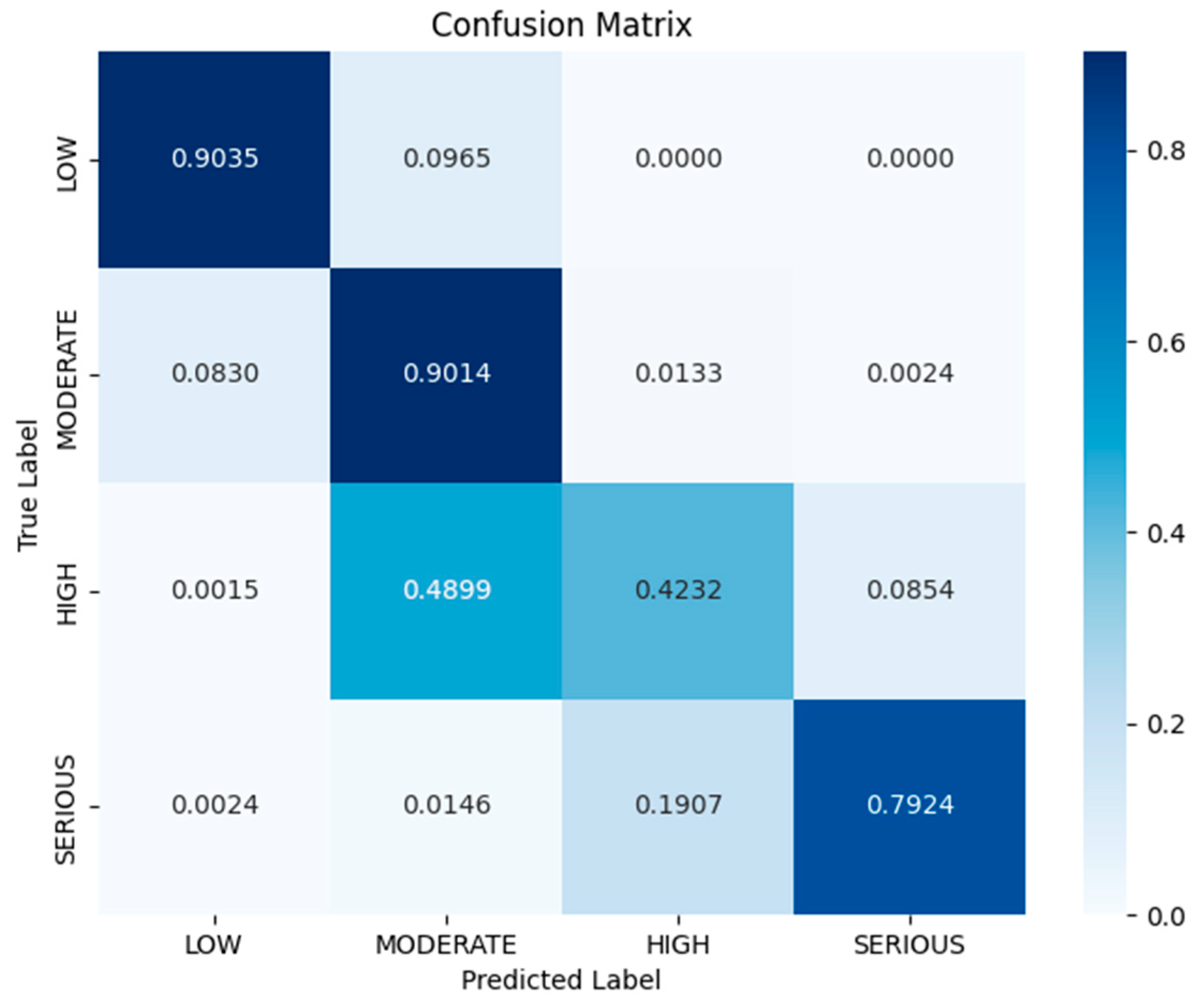
The BN model achieved an average accuracy of 87.14 percent, corresponding to an error rate of 12.86 percent, as shown in Table 5. This represents approximately a 10 percent lower accuracy compared to the MLP model. The classification accuracy for each risk level was evaluated through a confusion matrix in Figure 18. The results demonstrate that both low- and moderate-risk predictions exceeded 90 percent accuracy, with the primary misclassification occurring when low-risk cases were incorrectly labeled as moderate. However, high-risk prediction accuracy was notably lower at less than 50 percent, with nearly half of high-risk cases being misclassified as moderate. It can be seen that although the MLP model is less interpretable, it is much more accurate than the more interpretable BN model in terms of accuracy, especially in high classification.
Through sensitivity analysis performed using Genie software with flood risk as the target variable, we examined the influence of each parent node on flood risk outcomes as illustrated in Figure 19. The analysis revealed that land use shows a sensitivity value of 4.8 percent, ranking fourth among the seventeen parent nodes. However, this numerical ranking significantly underestimates land use’s actual impact. Land use exerts substantial influence on the top three most sensitive factors: nighttime lighting in first position, population density in second place, and gross product per unit area ranking third. These findings suggest that although there is no absolute advantage in direct sensitivity rankings, strategically altering land use can effectively mitigate flood risks.
Through systematic modification of land use probabilities within the trained BN model, we derived flood risk probability distributions across various land use scenarios, with results presented in Figure 20.
Figure 20A demonstrates that all three scenarios in the BN show elevated probabilities of serious, high, and moderate flood risks compared to the base year conditions. The urban construction scenario yields the highest probability of high flood risk at 6.215%. Among the scenarios, ecological preservation presents the most favorable risk profile, with the lowest probabilities of serious (6.136%) and high risk (11.132%), coupled with the highest probabilities of moderate (46.138%) and low risk (36.595%). The natural development scenario produces intermediate results, while the urban construction scenario generates the least favorable outcomes, exhibiting the highest probabilities of severe risks and the lowest probabilities of moderate and low risks. Figure 20B reveals that town development dominates the serious (33.546%) and high-risk (33.628%) categories, indicating these risk levels are primarily associated with urban expansion. Conversely, ecological protection accounts for the majority of moderate- and low-risk areas, demonstrating that conservation strategies effectively mitigate flood risks.

4.3.3. Flood Risk Index

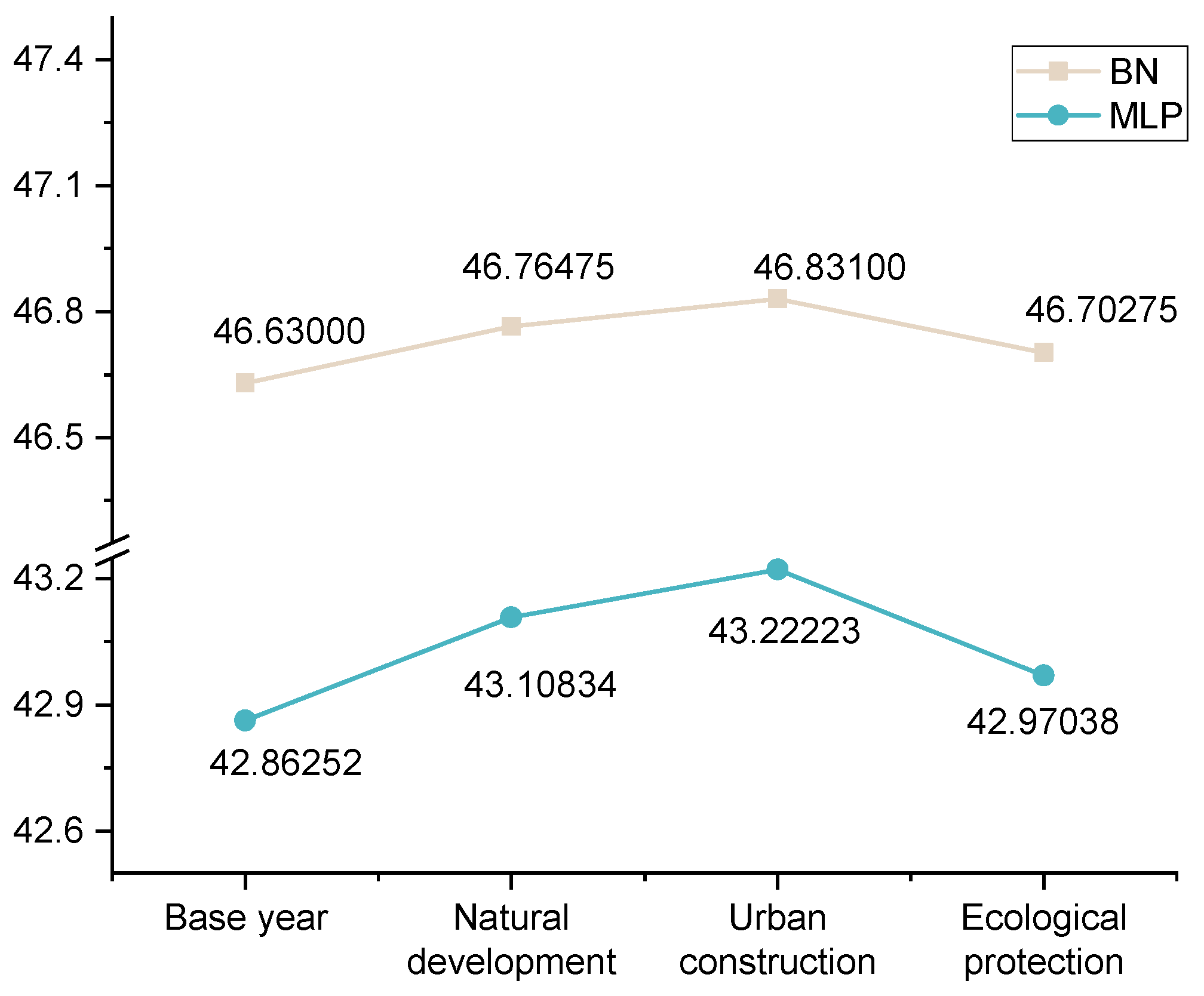
The simulation results demonstrate strong consistency between the two models. By applying Equation (16) to calculate flood risk indices for different scenarios, we obtained the results presented in Figure 21. While the absolute risk values differ between BN and MLP models due to their distinct network structures and computational logics, both models consistently show identical trends across scenarios. Specifically, the urban construction scenario yields the highest flood risk in both models, with indices of 46.83100 (BN) and 43.22230 (MLP). The natural development scenario ranks second, producing risk indices of 46.76475 (BN) and 43.10834 (MLP). The ecological protection scenario consistently shows the lowest risk, with corresponding values of 46.70275 (BN) and 42.97038 (MLP). Notably, all three scenarios exhibit higher risk indices compared to the base year conditions.

5. Discussion

5.1. Flood Risk Assessment

Flooding in the Dongting Lake basin and along the Xiang River has been extensively studied, with existing research focusing on flood resilience, flood damage assessment, and flood occurrence mechanisms [54,55]. The CZT urban agglomeration, located adjacent to these water bodies, faces particularly high flood risks due to increasing urban flood events in recent years. This study employs a multi-criteria indicator system to assess flood risk in this region, with results generally aligning with previous findings. These studies are similar in scope to our research and have been validated by historical flood locations, flood losses, historical flood areas, etc. [56,57,58]. However, our approach differs from prior studies in several key aspects. First, while many existing risk assessments omit resilience factors—a significant limitation given real-world conditions—our framework explicitly incorporates this critical dimension. Second, whereas previous work has often focused narrowly on specific aspects such as agricultural flood risk or urban/mountainous area flooding [59,60], our assessment comprehensively integrates both socioeconomic and natural factors. Third, regarding methodology, prior studies typically relied on either purely subjective or objective weighting approaches or their simple linear combinations. In contrast, we apply game theory to derive optimal combined weights, thereby enhancing model accuracy.

5.2. Probabilistic Flood Risk Prediction

Existing flood risk prediction studies have primarily focused on hydrological simulations to assess flood depths and risks under varying climate conditions and storm recurrence intervals [61,62], while largely neglecting the examination of flood risks associated with different land use scenarios. However, rapid urbanization has significantly amplified the influence of land use patterns on surface runoff processes. Incorporating land use considerations into flood risk assessment can provide effective mitigation strategies through optimized land planning. This study advances current methodologies by integrating the PLUS model with both BN and MLP approaches following initial risk assessment. Our coupled framework enables the prediction of both the probability and index of future flood risks across diverse land use scenarios. This novel integration facilitates the development of targeted land use policies for flood risk reduction, offering a more comprehensive approach to urban flood management. We have observed that while flood disasters vary under different land use scenarios, the overall risk changes relatively little. This can be attributed to several factors. First, the CZT urban agglomeration is located in the hilly regions of southern China, where forest land accounts for a significant proportion of the total land area, resulting in overall flood risk changing relatively little. However, when focusing on the Xiang River basin, we find that local land use changes are significant, leading to substantial increases in flood risk variability. This aligns with China’s governance framework, where government administrators at different levels can formulate appropriate policies based on the extent of local land use changes—crucial for mitigating urban flooding. Furthermore, the impact of land use on flood risk is not singular; land use also affects other risk factors. Including such interactions could further highlight land use’s influence, as researchers have demonstrated that it is a key factor affecting flood disasters [63].

5.3. Policy Recommendations

The flood risk assessment of the CZT urban agglomeration demonstrates that areas along both banks of the Xiang River exhibit significantly higher flood vulnerability compared to other regions, particularly within the zone’s economically developed urban cores. These densely urbanized areas, where construction land already predominates, present limited opportunities for flood risk reduction through large-scale land use changes due to both practical constraints and prohibitive costs. In such contexts, the most viable mitigation strategies should focus on enhancing drainage system capacity and optimizing the use of underground space while prioritizing the redevelopment of underutilized urban parcels over expansion into new areas. The findings highlight the profound impact of land use decisions on flood risk. Moving toward sustainable development requires a concerted effort to preserve and expand ecological lands, with particular emphasis on protecting existing forested areas and strengthening the ecological integrity of the metropolitan area’s designated “Green Heart.” This approach enables continued economic development while maintaining flood risk at acceptable levels through careful land use optimization rather than spatial expansion. Future urban development should strategically balance growth needs with hydrological considerations, ensuring that new construction occurs only after thorough evaluation of flood risk implications and with appropriate mitigation measures in place. Strict adherence to existing ecological protection policies will be essential for achieving this balance.

5.4. Innovations and Limitations

This study advances flood risk assessment methodology through several key innovations. First, we enhanced weight determination accuracy by integrating both subjective and objective weighting approaches, harmonizing them through game theory to achieve optimal balance. For flood risk prediction, we developed a novel coupling approach combining the PLUS model with both MLP and BN methods. The MLP model, augmented with SHAP analysis, effectively identifies the most influential risk factors, while the BN model provides complementary insights through sensitivity analysis. This dual-model approach not only improves predictive accuracy but also enhances result interpretability and robustness, as the mutually corroborating outputs from both MLP and BN models create a more reliable and comprehensive risk assessment framework.
The current analysis focuses specifically on land use impacts on flood risk, while recognizing that a more comprehensive assessment of interacting indicators would better reflect the complex dynamics of flood systems in natural environments. Methodologically, BN and MLP models were selected for risk probability prediction, though numerous alternative machine learning and deep learning approaches capable of processing categorical data remain to be systematically evaluated. In addition, different rainfall intensities, soil characteristics, and future climate change have not been taken into account, which will have an uncertain impact on our research. Future work should prioritize three areas: deeper investigation of how factor interactions influence flood risk, rigorous comparison of alternative predictive models to identify optimal approaches for accuracy improvement, and include broader environmental factors in the study. Such advancements would build upon the present findings while addressing current methodological constraints, ultimately leading to more robust flood risk assessment frameworks.

6. Conclusions

The flood risk assessment for the CZT urban agglomeration was conducted using the H-E-V-R framework. This study employed coupled modeling approaches, integrating the PLUS model with both BN and MLP techniques to predict future flood risks under various land use scenarios. The analysis yielded several key findings regarding regional flood risk:
(1) The high-risk areas for flood disasters in the CZT urban agglomeration exhibit significant spatial clustering, primarily concentrated along the Xiang River in the central part of the study area. Additionally, several discrete high-risk patches are distributed across the eastern and western regions. In contrast, low-risk areas are predominantly characterized by a scattered distribution, mainly located in hilly and mountainous terrain distant from urban agglomeration and core economic zones.
(2) The PLUS model was employed to simulate future land use in the CZT urban agglomeration, achieving a Kappa coefficient of 0.78 and an overall accuracy of 0.87, which satisfies the requirements for reliable simulation. Among the three scenarios analyzed, only the ecological protection scenario demonstrates a modest increase in forested land area, rising from 9501.61 km2 to 9534.45 km2 compared to the baseline year of 2023. This suggests that ecological protection policies effectively enhance forest retention. Meanwhile, while cultivated land area decreases by 173.19 km2 relative to the natural development scenario, it remains significantly higher than under the urban development scenario, highlighting the positive role of this scenario in preserving agricultural production. Additionally, the ecological protection scenario effectively controls construction land expansion, resulting in the smallest reductions in grassland and water areas, as well as the least increase in construction land among the three scenarios.
(3) The flood risk in the CZT urban agglomeration under future scenarios was predicted using MLP and BN models, with accuracies of 97.83% and 87.14%, respectively. The results demonstrate that land use significantly influences flood risk. Among the scenarios analyzed, the ecological protection scenario exhibits the lowest flood risk, followed by the natural development scenario, while the urban construction scenario presents the highest risk. These findings indicate that ecological protection policies are more effective in mitigating flood risk, underscoring the practical significance of land use planning in flood risk reduction.

Author Contributions

Conceptualization, T.Z. and K.W.; methodology, T.Z.; software, T.Z. and L.C.; validation, T.Z. and K.W.; formal analysis, T.Z.; investigation, T.Z. and X.W.; resources, T.Z. and K.W.; data curation, T.Z.; writing—original draft preparation, T.Z., K.W., X.W., X.L., L.L. and L.C.; writing—review and editing, T.Z. and K.W.; visualization, T.Z., K.W., X.W. and L.C.; supervision, T.Z., K.W., X.L., L.L. and L.C.; project administration, K.W.; funding acquisition, L.L. All authors have read and agreed to the published version of the manuscript.

Funding

This research was supported by the National Natural Science Foundation of China Youth Science Fund Program (42001212); the Special Fund Project for Geological Exploration Construction and Development in Shanxi Province—Open Fund of Shanxi Geoscience Think Tank (2023-008); and the Science and Technology Innovation Project of Jiangsu Provincial Department of Natural Resources (2022008).

Data Availability Statement

Data will be made available on request. The data are not publicly available due to privacy.

Acknowledgments

We gratefully acknowledge the anonymous reviewers and the editors for their comments and suggestions that improved this manuscript.

Conflicts of Interest

The authors declare no conflicts of interest.

References

  1. Tellman, B.; Sullivan, J.A.; Kuhn, C.; Kettner, A.J.; Doyle, C.S.; Brakenridge, G.R.; Erickson, T.A.; Slayback, D.A. Satellite imaging reveals increased proportion of population exposed to floods. Nature 2021, 596, 80–86. [Google Scholar] [CrossRef]
  2. Bhere, S.; Reddy, M.J. Flood risk assessment of suburban region in India by incorporating flood hazard, vulnerability and exposure. Nat. Hazards 2025, 121, 6625–6649. [Google Scholar] [CrossRef]
  3. Park, K.; Lee, E.H. Urban flood vulnerability analysis and prediction based on the land use using Deep Neural Network. Int. J. Disaster Risk Reduct. 2024, 101, 104231. [Google Scholar] [CrossRef]
  4. Dong, B.L.; Xia, J.Q.; Wang, X.J. Comprehensive flood risk assessment in highly developed urban areas. J. Hydrol. 2025, 648, 132391. [Google Scholar] [CrossRef]
  5. Feng, J.; Tian, Y.; Xie, Z.L.; Wang, H. Risk Assessment of Campus Waterlogging and Evacuation Route Planning. Water Resour. Manag. 2025, 39, 3071–3107. [Google Scholar] [CrossRef]
  6. Fu, G.T.; Meng, F.L.; Casado, M.R.; Kalawsky, R.S. Towards Integrated Flood Risk and Resilience Management. Water 2020, 12, 1789. [Google Scholar] [CrossRef]
  7. Zhang, J.W.; Wang, J.G.; Chen, S.B.; Tang, S.Q.; Zhao, W.T. Multi-Hazard Meteorological Disaster Risk Assessment for Agriculture Based on Historical Disaster Data in Jilin Province, China. Sustainability 2022, 14, 7482. [Google Scholar] [CrossRef]
  8. Benito, G.; Castillo, O.; Ballesteros-Cánovas, J.A.; Machado, M.; Barriendos, M. Enhanced flood hazard assessment beyond decadal climate cycles based on centennial historical data (Duero basin, Spain). Hydrol. Earth Syst. Sci. 2021, 25, 6107–6132. [Google Scholar] [CrossRef]
  9. Mainguenaud, F.; Khan, U.T.; Peyras, L.; Carvajal, C.; Beullac, B.; Sharma, J. Probabilistic Flood Hazard Assessment for Multiple Flood and Levee Breaching Scenarios: A Case Study of Etobicoke Creek, Canada. J. Flood Risk Manag. 2025, 18, e70002. [Google Scholar] [CrossRef]
  10. Liu, W.; Zhang, X.; Feng, Q.; Engel, B.A. City-scale integrated flood risk prediction under future climate change and urbanization based on the shared socioeconomic pathways (SSP) scenarios. J. Hydrol. 2025, 655, 132971. [Google Scholar] [CrossRef]
  11. Tanim, A.H.; Smith-Lewis, C.; Downey, A.; Imran, J.; Goharian, E. Bayes_Opt-SWMM: A Gaussian process-based Bayesian optimization tool for real-time flood modeling with SWMM. Environ. Modell. Softw. 2024, 179, 106122. [Google Scholar] [CrossRef]
  12. Zischg, A.P.; Mosimann, M.; Bernet, D.B.; Röthlisberger, V. Validation of 2D flood models with insurance claims. J. Hydrol. 2018, 557, 350–361. [Google Scholar] [CrossRef]
  13. Zhao, L.; Zhang, T.; Fu, J.; Li, J.; Cao, Z.; Feng, P. Risk Assessment of Urban Floods Based on a SWMM-MIKE21-Coupled Model Using GF-2 Data. Remote Sens. 2021, 13, 4381. [Google Scholar] [CrossRef]
  14. Bhuyan, M.J.; Deka, N.; Saikia, A. Micro-spatial flood risk assessment in Nagaon district, Assam (India) using GIS-based multi-criteria decision analysis (MCDA) and analytical hierarchy process (AHP). Risk Anal. 2024, 44, 817–832. [Google Scholar] [CrossRef] [PubMed]
  15. Chen, Y.R.; Zhang, N.; Zhang, X.L.; Wang, G.P.; Wang, Y.; Liu, R.H.; Ma, M.H. A novel dynamic flash flood early warning framework based on distributed hydrologic modeling. Ecol. Indic. 2025, 172, 113247. [Google Scholar] [CrossRef]
  16. Hossain, M.N.; Mumu, U.H. Flood susceptibility modelling of the Teesta River Basin through the AHP-MCDA process using GIS and remote sensing. Nat. Hazards 2024, 120, 12137–12161. [Google Scholar] [CrossRef]
  17. Nkonu, R.S.; Antwi, M. A novel ANN-CA and MCDA integrated framework for predicting urban expansion and its implications on future flood risk, Accra Metropolis. Environ. Dev. 2024, 52, 101061. [Google Scholar] [CrossRef]
  18. Fang, X.Q.; Liao, M.Y.; Yang, L.L.; Jiang, X.Y.; Jin, J.X.; Zhu, Q. Assessment of Flash Flood Risk Using Random Forest Regression Model Integrated with Binary Statistics. In Proceedings of the IGARSS 2024-2024 IEEE International Geoscience and Remote Sensing Symposium, Athens, Greece, 7–12 July 2024; pp. 3952–3955. [Google Scholar]
  19. Lu, Y.; Zhai, G.; Zhou, S. An integrated Bayesian networks and Geographic information system (BNs-GIS) approach for flood disaster risk assessment: A case study of Yinchuan, China. Ecol. Indic. 2024, 166, 112322. [Google Scholar] [CrossRef]
  20. Wang, Y.L.; Tian, Z.; Zhang, S.Y.; Guan, Y.L.; Ke, Q.; Yang, H.L. Flood risk assessment by heterogeneous ensemble learning techniques: A case study of Shenzhen City, China. J. Hydrol. 2025, 650, 132566. [Google Scholar] [CrossRef]
  21. Wei, Q.; Zhang, H.J.; Chen, Y.Q.; Xie, Y.F.; Yin, H.L.; Xu, Z.X. City scale urban flooding risk assessment using multi-source data and machine learning approach. J. Hydrol. 2025, 651, 132626. [Google Scholar] [CrossRef]
  22. Li, G.Y.; Shao, W.W.; Su, X.; Li, Y.; Zhang, Y.; Song, T.X. Urban Flood Hazard Assessment Based on Machine Learning Model. Water Resour. Manag. 2025, 39, 1953–1970. [Google Scholar] [CrossRef]
  23. Ding, J.W.; Wang, X.K.; Zhou, S.F.; Lei, S. Holistic risk assessment using a hybrid approach in a flash flood disaster-prone area of the Poyang lake basin. Nat. Hazards 2025, 121, 12959–12984. [Google Scholar] [CrossRef]
  24. Zhang, M.J.; Fu, X.; Liu, S.J.; Zhang, C. Integrating Remote Sensing and Machine Learning for Actionable Flood Risk Assessment: Multi-Scenario Projection in the Ili River Basin in China Under Climate Change. Remote Sens. 2025, 17, 1189. [Google Scholar] [CrossRef]
  25. Pradhan, B.; Lee, S.; Dikshit, A.; Kim, H. Spatial flood susceptibility mapping using an explainable artificial intelligence (XAI) model. Geosci. Front. 2023, 14, 101625. [Google Scholar] [CrossRef]
  26. Singha, C.; Sahoo, S.; Mahtaj, A.B.; Moghimi, A.; Welzel, M.; Govind, A. Advancing flood risk assessment: Multitemporal SAR-based flood inventory generation using transfer learning and hybrid fuzzy-AHP-machine learning for flood susceptibility mapping in the Mahananda River Basin. J. Environ. Manag. 2025, 380, 124972. [Google Scholar] [CrossRef]
  27. Lou, Y.H.; Wang, P.; Li, Y.; Zhang, Y.D.; Xie, B.; Hu, T.A. Projecting urban flood risk through hydrodynamic modeling under shared socioeconomic pathways. J. Environ. Manag. 2024, 370, 122647. [Google Scholar] [CrossRef]
  28. Allegri, E.; Zanetti, M.; Torresan, S.; Critto, A. Pluvial flood risk assessment for 2021–2050 under climate change scenarios in the Metropolitan City of Venice. Sci. Total Environ. 2024, 914, 169925. [Google Scholar] [CrossRef] [PubMed]
  29. Luo, P.P.; Wang, X.H.; Zhang, L.; Zainol, M.; Duan, W.L.; Hu, M.C.; Guo, B.; Zhang, Y.Z.; Wang, Y.H.; Nover, D. Future Land Use and Flood Risk Assessment in the Guanzhong Plain, China: Scenario Analysis and the Impact of Climate Change. Remote Sens. 2023, 15, 5778. [Google Scholar] [CrossRef]
  30. Zhao, H.B.; Gu, T.S.; Tang, J.Q.; Gong, Z.Y.; Zhao, P.J. Urban flood risk differentiation under land use scenario simulation. iScience 2023, 26, 106479. [Google Scholar] [CrossRef] [PubMed]
  31. Lin, W.; Sun, Y.; Nijhuis, S.; Wang, Z. Scenario-based flood risk assessment for urbanizing deltas using future land-use simulation (FLUS): Guangzhou Metropolitan Area as a case study. Sci. Total Environ. 2020, 739, 139899. [Google Scholar] [CrossRef] [PubMed]
  32. Acuña-Alonso, C.; Alvarez, X.; Bezak, N.; Zupanc, V. Modelling the impact land use change on flood risk: Umia (Spain) and Voglajna (Slovenia) case studies. Ecol. Eng. 2024, 200, 107185. [Google Scholar] [CrossRef]
  33. Situ, Z.; Zhong, Q.S.; Zhang, J.L.; Teng, S.; Ge, X.G.; Zhou, Q.Q.; Zhao, Z.W. Attention-based deep learning framework for urban flood damage and risk assessment with improved flood prediction and land use segmentation. Int. J. Disaster Risk Reduct. 2025, 116, 105165. [Google Scholar] [CrossRef]
  34. Sun, Q.; Fang, J.; Dang, X.; Xu, K.; Fang, Y.; Li, X.; Liu, M. Multi-scenario urban flood risk assessment by integrating future land use change models and hydrodynamic models. Nat. Hazards Earth Syst. Sci. 2022, 22, 3815–3829. [Google Scholar] [CrossRef]
  35. Liu, J.; Wang, J.; Xiong, J.; Cheng, W.; Cui, X.; He, W.; He, Y.; Duan, Y.; Yang, G.; Wang, N. Dynamic Assessment of the Flood Risk at Basin Scale under Simulation of Land-Use Scenarios and Spatialization Technology of Factor. Water 2021, 13, 3239. [Google Scholar] [CrossRef]
  36. Abijith, D.; Saravanan, S.; Parthasarathy, K.S.S.; Reddy, N.M.; Niraimathi, J.; Bindajam, A.A.; Mallick, J.; Alharbi, M.M.; Abdo, H.G. Assessing the impact of climate and land use change on flood vulnerability: A machine learning approach in coastal region of Tamil Nadu, India. Geosci. Lett. 2025, 12, 1. [Google Scholar] [CrossRef]
  37. Wind, E. Zhuzhou 7–8 Days of Heavy Rainstorms Followed by Sunny Days to Warm Up. Available online: https://baijiahao.baidu.com/s?id=1831342132050851664&wfr=spider&for=pc (accessed on 15 December 2024).
  38. Na, W. Typhoon “Memo” in Zhuzhou. Available online: https://baijiahao.baidu.com/s?id=1806507868216377868&wfr=spider&for=pc (accessed on 13 August 2025).
  39. Wu, H.P. 36 Townships (Streets) and 76,379 People Were Affected in Xiangtan! Floods Hit, They Defend Their Homes like This! Pescadores. Xiangtan, 2019. Available online: https://m.thepaper.cn/baijiahao_3911171 (accessed on 16 December 2024).
  40. Che, L.S.; Yin, S.Y.; Guo, Y.S. Flood risk assessment combining the historical disaster statistics method with the index system method. Hydrol. Sci. J. 2025, 70, 510–521. [Google Scholar] [CrossRef]
  41. Pham, B.T.; Luu, C.; Dao, D.V.; Phong, T.V.; Nguyen, H.D.; Le, H.V.; von Meding, J.; Prakash, I. Flood risk assessment using deep learning integrated with multi-criteria decision analysis. Knowl.-Based Syst. 2021, 219, 106899. [Google Scholar] [CrossRef]
  42. Zhang, T.; Wang, X.L.; Li, X.A.; Zhu, X.; Li, L.; Chen, L.Q. Spatio-Temporal Differentiation and Influencing Factors of Urban Ecological Resilience in Xuzhou City. Land 2025, 14, 1048. [Google Scholar] [CrossRef]
  43. Zhang, D.; Shi, X.; Xu, H.; Jing, Q.; Pan, X.; Liu, T.; Wang, H.; Hou, H. A GIS-based spatial multi-index model for flood risk assessment in the Yangtze River Basin, China. Environ. Impact Assess. Rev. 2020, 83, 106397. [Google Scholar] [CrossRef]
  44. Sun, R.; Shi, S.; Reheman, Y.; Li, S. Measurement of urban flood resilience using a quantitative model based on the correlation of vulnerability and resilience. Int. J. Disaster Risk Reduct. 2022, 82, 103344. [Google Scholar] [CrossRef]
  45. Whittingham, M.J.; Stephens, P.A.; Bradbury, R.B.; Freckleton, R.P. Why do we still use stepwise modelling in ecology and behaviour? J. Anim. Ecol. 2006, 75, 1182–1189. [Google Scholar] [CrossRef]
  46. Li, L.; Zhou, X.S.; Chen, L.Q.; Chen, L.G.; Zhang, Y.; Liu, Y.Q. Estimating Urban Vegetation Biomass from Sentinel-2A Image Data. Forests 2020, 11, 125. [Google Scholar] [CrossRef]
  47. Mutale, B.; Qiang, F. Modeling future land use and land cover under different scenarios using patch-generating land use simulation model. A case study of Ndola district. Front. Environ. Sci. 2024, 12, 1362666. [Google Scholar] [CrossRef]
  48. Teng, G.; Chen, L.Q.; Zhang, T.; Li, L.; Xiao, J.; Ma, L.Y. The Spatiotemporal Evolution of Land Use Ecological Efficiency in the Huaihai Economic Zone: Insights from a Multi-Dimensional Framework and Geospatial Modeling. Land 2025, 14, 883. [Google Scholar] [CrossRef]
  49. Tang, L.S.; Li, J.Z.; Xie, C.M.; Wang, M. Multi-Scenario Simulation of Ecosystem Service Value in Xiangjiang River Basin, China, Based on the PLUS Model. Land 2025, 14, 1482. [Google Scholar] [CrossRef]
  50. Zhou, W.; Wang, J.; Han, Y.; Yang, L.; Que, H.; Wang, R. Scenario Simulation of the Relationship between Land-Use Changes and Ecosystem Carbon Storage: A Case Study in Dongting Lake Basin, China. Int. J. Environ. Res. Public Health 2023, 20, 4835. [Google Scholar] [CrossRef] [PubMed]
  51. Bakhtiari, S.; Najafi, M.R.; Goda, K.; Peerhossaini, H. Integrated Bayesian Network and Strongest Path Method (BN-SPM) for effective multi-hazard risk assessment of interconnected infrastructure systems. Sust. Cities Soc. 2024, 104, 105294. [Google Scholar] [CrossRef]
  52. Banan-Dallalian, M.; Shokatian-Beiragh, M.; Golshani, A.; Abdi, A. Use of a Bayesian Network for storm-induced flood risk assessment and effectiveness of ecosystem-based risk reduction measures in coastal areas (Port of Sur, Sultanate of Oman). Ocean Eng. 2023, 270, 113662. [Google Scholar] [CrossRef]
  53. Kjærulff, U.; van der Gaag, L.C. Making Sensitivity Analysis Computationally Efficient. In Proceedings of the Sixteenth Conference On Uncertainty In Artificial Intelligence, San Francisco, CA, USA, 30 June–3 July 2000; Morgan Kaufmann Publishers Inc.: San Francisco, CA, USA, 2000. [Google Scholar]
  54. Yu, S.Y.; Kong, X.S.; Wang, Q.; Yang, Z.W.; Peng, J. A new approach of Robustness-Resistance-Recovery (3Rs) to assessing flood resilience: A case study in Dongting Lake Basin. Landsc. Urban Plan. 2023, 230, 104605. [Google Scholar] [CrossRef]
  55. Yan, R.; Liu, L.L.; Wang, J.; Zhou, S.; Wu, S.H. Assessment of flood loss in administrative units based on improved vulnerability curves. Adv. Clim. Change Res. 2025, 16, 154–166. [Google Scholar] [CrossRef]
  56. Wang, Y.M.; Li, Z.W.; Tang, Z.H.; Zeng, G.M. A GIS-Based Spatial Multi-Criteria Approach for Flood Risk Assessment in the Dongting Lake Region, Hunan, Central China. Water Resour. Manag. 2011, 25, 3465–3484. [Google Scholar] [CrossRef]
  57. Yang, M.; Yusoff, W.; Mohamed, M.F.; Jiao, S.; Dai, Y.J. Flood economic vulnerability and risk assessment at the urban mesoscale based on land use: A case study in Changsha, China. J. Environ. Manag. 2024, 351, 119798. [Google Scholar] [CrossRef] [PubMed]
  58. Zhou, S.H.; Xu, Z.W.; Zhang, Q.S.; Yu, P.; Jiang, M.Y.; Li, J.F.; Yang, M.H. Rainstorm-induced flood risk assessment in developed urban area using a data-driven approach with watershed units. Sci. Total Environ. 2024, 946, 174135. [Google Scholar] [CrossRef] [PubMed]
  59. Baggio, T.; Martini, M.; Bettella, F.; D’Agostino, V. Debris flow and debris flood hazard assessment in mountain catchments. CATENA 2024, 245, 108338. [Google Scholar] [CrossRef]
  60. Bin, L.L.; Xu, K.; Pan, H.; Zhuang, Y.C.; Shen, R.Z. Urban flood risk assessment characterizing the relationship among hazard, exposure, and vulnerability. Environ. Sci. Pollut. Res. 2023, 30, 86463–86477. [Google Scholar] [CrossRef]
  61. Zeng, Z.Y.; Lai, C.G.; Wang, Z.L.; Chen, Y.H.; Chen, X.H. Future sea level rise exacerbates compound floods induced by rainstorm and storm tide during super typhoon events: A case study from Zhuhai, China. Sci. Total Environ. 2024, 911, 168799. [Google Scholar] [CrossRef]
  62. Smits, W.K.; Attoh, E.; Ludwig, F. Flood risk assessment and adaptation under changing climate for the agricultural system in the Ghanaian White Volta Basin. Clim. Change 2024, 177, 39. [Google Scholar] [CrossRef]
  63. Nguyen, H.D.; Dang, D.K.; Nguyen, Q.H.; Bui, Q.T.; Petrisor, A.I. Evaluating the effects of climate and land use change on the future flood susceptibility in the central region of Vietnam by integrating land change modeler, machine learning methods. Geocarto Int. 2022, 37, 12810–12845. [Google Scholar] [CrossRef]
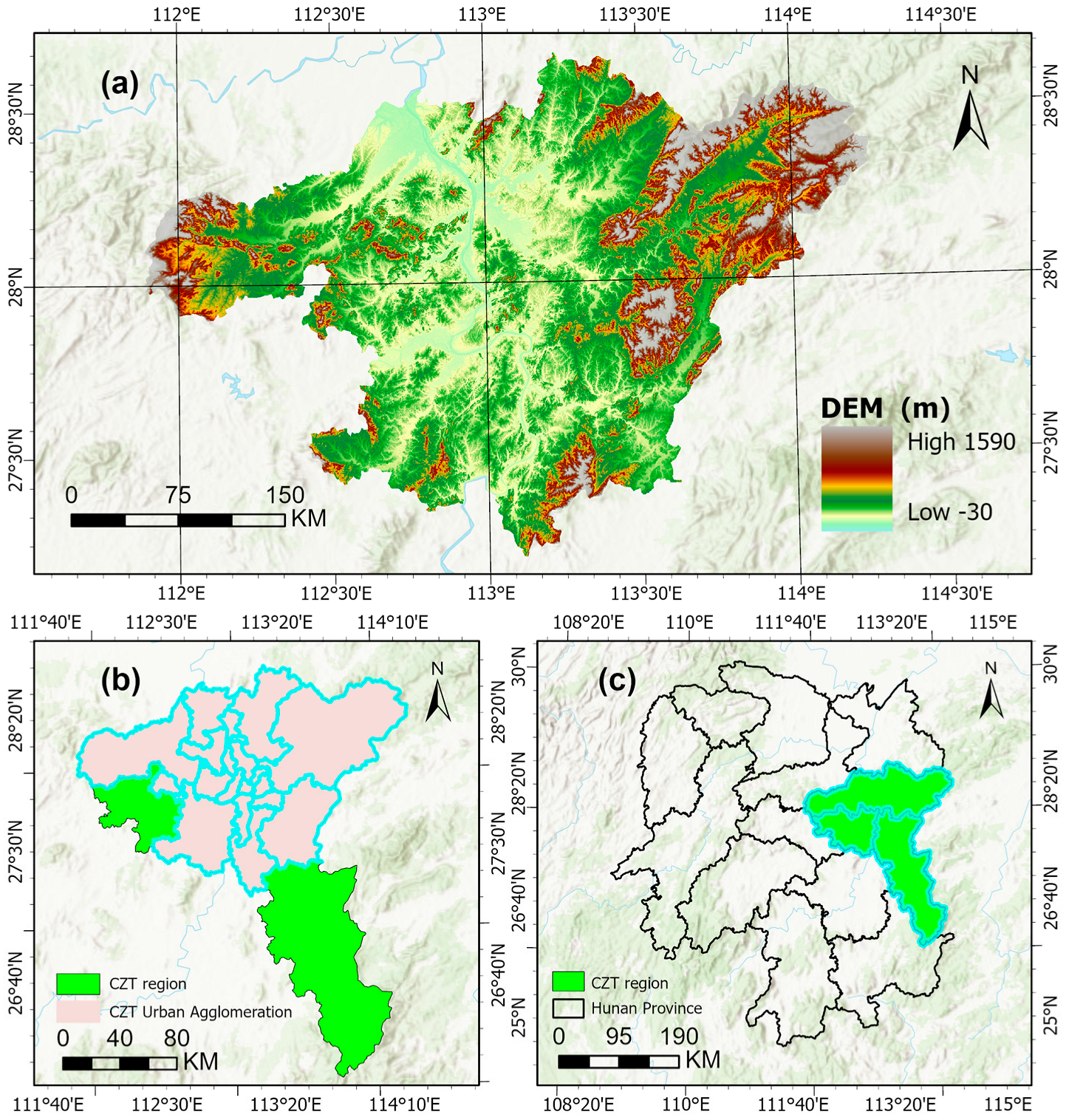
Figure 1. Schematic map of the scope and geographic location of CZT urban agglomeration. (a) Administrative division and elevation of CZT urban agglomeration; (b) location of CZT urban agglomeration in the three cities of CZT; (c) location of the three cities of CZT in Hunan Province.
Remotesensing 17 02889 g001
Figure 2. Research framework.
Remotesensing 17 02889 g002
Figure 3. Structure of the MLP model (Ai, Bi, and Ci represent neurons, and Yi represents the output result).
Remotesensing 17 02889 g003
Figure 4. Schematic diagram of the softmax function (P represents the probability vector, and A, B, and C are the raw numerical values output by the model).
Remotesensing 17 02889 g004
Figure 5. BN model for predicting the probability of flood risk.
Remotesensing 17 02889 g005
Figure 6. Flood hazard ranking of CZT urban agglomeration.
Remotesensing 17 02889 g006
Figure 7. Flood exposure ranking of CZT urban agglomeration.
Remotesensing 17 02889 g007
Figure 8. Flood vulnerability ranking of CZT urban agglomeration.
Remotesensing 17 02889 g008
Figure 9. Flood resilience ranking map of CZT urban agglomeration.
Remotesensing 17 02889 g009
Figure 10. Distribution of assessment results at the criterion layer.
Remotesensing 17 02889 g010
Figure 11. Flood risk ranking of CZT urban agglomeration.
Remotesensing 17 02889 g011
Figure 12. Changes in the amount of land use under different land use scenarios, 2020–2035.
Remotesensing 17 02889 g012
Figure 13. Land use in 2020 and simulated land use for the year 2035 under three different land use scenarios.
Remotesensing 17 02889 g013
Figure 14. MLP model training and test set accuracies (left panel) and loss curves (right panel).
Remotesensing 17 02889 g014
Figure 15. MLP model confusion matrix.
Remotesensing 17 02889 g015
Figure 16. Probability of flood risk for different land use scenarios of the MLP model. (A) Probability of flood risk under land use scenarios. (B) Probability of land use scenarios under flood risk.
Remotesensing 17 02889 g016
Figure 17. Summary plot of SAHP values for the MLP model.
Remotesensing 17 02889 g017
Figure 18. BN model confusion matrix.
Remotesensing 17 02889 g018
Figure 19. Target node sensitivity.
Remotesensing 17 02889 g019
Figure 20. Probability of flood risk for different land use scenarios of the BN model. (A) Probability of flood risk under land use scenarios. (B) Probability of land use scenarios under flood risk.
Remotesensing 17 02889 g020
Figure 21. Flood risk index.
Remotesensing 17 02889 g021
Table 1. Data used in the study.
Data and IndicatorResolutionData Source
Mean annual
precipitation and temperature station data
/National Oceanic and Atmospheric Administration: https://www.ncei.noaa.gov/data/global-summary-of-the-day/archive/ accessed on 13 August 2025
Nighttime light intensity250 m × 250 m
DEM12.5 m × 12.5 mNASA: https://www.nasa.gov/ accessed on 13 August 2025
Slope30 m × 30 mExtracted DEM
River network density
NDVI250 m × 250 mMODIS Imagery (2014–2023 MOD09Q1 Products) Extraction: https://ladsweb.modaps.eosdis.nasa.gov/search/ accessed on 13 August 2025
Flooding frequency
Population density1 km × 1 kmLandScan data from the U.S. Department of Energy’s Oak Ridge National Laboratory: https://landscan.ornl.gov accessed on 13 August 2025
GDP per unit area1 km × 1 kmResource and Environmental Science and Data
Center, Chinese Academy of Sciences: https://www.resdc.cn/ accessed on 13 August 2025
Distance from the drainage network30 m × 30 mOpen Street Map: https://www.openstreetmap.org/ accessed on 13 August 2025
Road network density
Land useThe Wuhan University CLCD dataset: https://doi.org/10.5281/zenodo.4417809 accessed on 13 August 2025
Per capita disposable income/Statistical Yearbook of Hunan Province and Chang-Zhu-Tan Three Cities
Number of healthcare workers
Public revenues
Number of primary school students
Number of elderly people
Distance from first-class, second-class, and third-class roads, distance from the district/county center, distance from highway, distance from the railway30 m × 30 mEuclidean Distance Analysis by Open Street Map Data
Administrative districts/National Platform for Common GeoSpatial Information Services: https://cloudcenter.tianditu.gov.cn/administrativeDivision accessed on 13 August 2025
Table 2. Results of multicollinearity test.
IndicatorVIFIndicatorVIF
Mean annual precipitation (X1)1.69Number of elderly people (X10)4.03
DEM (X2)2.61Road network density (X11)3.62
Relative DEM (X3)2.54NDVI (X12)2.75
Flooding frequency (X4)1.04Land use (X13)2.34
Population density (X5)2.08Per capita disposable income (X14)4.37
River network density (X6)1.34Number of healthcare workers (X15)8.93
GDP per unit area (X7)2.39Public revenues (X16)7.43
Nighttime light intensity (X8)4.02Distance from the drainage network (X17)1.45
Number of primary school students (X9)4.33
Table 3. Indicator system weights.
Criterion LayerIndicator LayerAHPEWGTImpact on Criterion Layer
HMean annual precipitation0.10170.00340.0448+
DEM0.07090.06710.0687
Relative DEM0.0620.02630.0413
Flooding frequency0.07440.16860.1289+
EPopulation density0.04160.13310.0946+
River network density0.04900.00890.0258+
GDP per unit area0.02900.09670.0682+
Nighttime light intensity0.01880.12410.0797+
VNumber of primary school students0.06100.05440.0572+
Number of elderly people0.02250.04830.0375+
Road network density0.04440.07610.0628+
NDVI0.04410.02030.0303/
Land use0.04820.07120.0614/
RPer capita disposable income0.16570.03390.0894+
Number of healthcare workers0.06950.02270.0424+
Public revenues0.04240.02570.0327+
Distance from the drainage network0.05480.01920.0342
Table 4. Grading of BN and MLP data.
DataGrade
LowModerateHighSerious
Mean annual precipitation<1826.51826.5–1919.61919.6–2000.1>2000.1
DEM>12080–12040–80<40
Relative DEM>18.110.5–18.14.8–10.5<4.5
Flooding frequency<11–33–5>5
Population density<13231323–45424542–11,438>11,438
River network density<0.0530.053–0.1250.125–0.199>0.199
GDP per unit area<82078207–33,05333,053–105,221>105,221
Nighttime light intensity<5.975.97–19.5219.52–38.14>38.14
Number of primary school students<30,66730,667–48,17548,175–82,50682,506
Number of elderly people<61,65761,657–95,68295,682–150,218>95,682
Road network density<0.460.46–1.261.26–2.55>2.55
NDVI>0.630.49–0.630.33–0.49<0.33
Land useForest, othersFarmland, grasslandWater bodyBuilt-up land
Per capita disposable income>54,86647,763–54,86632,626–47,763<32,626
Number of healthcare workers>10,1106848–10,1102909–6848<2909
Public revenues>1,011,440393,730–1,011,440161,072–393,730<393,730
Distance from the drainage network<9652.999652.99–21,038.5721,038.57–35,889.33>35,889.33
Hazard<0.350.35–0.460.46–0.55>0.55
Exposure<0.030.03–0.080.08–0.15>0.15
Vulnerability<0.110.11–0.250.25–0.50>0.50
Resilience>0.740.53–0.740.32–0.53<0.32
Flood risk<0.080.08–0.260.26–0.50>0.50
Table 5. The results of the MLP model training based on a 10-fold cross-validation.
Fold n12345678910Average
Error rate (%)2.132.112.152.072.252.052.192.311.872.632.17
Table 6. The results of the BN model training based on a 10-fold cross-validation.
Fold n12345678910Average
Error rate (%)12.5612.4611.9412.7412.213.5313.8514.0312.2812.9812.86
Disclaimer/Publisher’s Note: The statements, opinions and data contained in all publications are solely those of the individual author(s) and contributor(s) and not of MDPI and/or the editor(s). MDPI and/or the editor(s) disclaim responsibility for any injury to people or property resulting from any ideas, methods, instructions or products referred to in the content.