A Hybrid Short-Term Prediction Model for BDS-3 Satellite Clock Bias Supporting Real-Time Applications in Data-Denied Environments

Abstract

High-precision satellite clock bias (SCB) prediction is essential for GNSS applications, including real-time precise point positioning (RT-PPP), Earth observation, planetary exploration, and spaceborne geodetic missions. However, during communication outages or when real-time SCB products are unavailable, RT-PPP may fail due to missing clock corrections. This underscores the necessity of reliable short-term SCB prediction in data-denied environments. To address this challenge, a hybrid model that integrates wavelet transform, a particle swarm optimization-enhanced gray model, and a first-order weighted local method is proposed for short-term SCB prediction. First, the novel model employs the db1 wavelet to perform three-level multi-resolution decomposition and single-branch reconstruction on preprocessed SCB, yielding one trend term and three detailed terms. Second, the particle swarm optimization algorithm is adopted to globally optimize the parameters of the traditional gray model to avoid falling into local optima, and the optimization-enhanced gray model is applied to predict the trend term. For the three detailed terms, the embedding dimension and time delay are calculated, and they are constructed in phase space to establish a first-order weighted local model for prediction. Third, the final SCB prediction is obtained by summing the predicted results of the trend term and the three detailed terms correspondingly. The BDS-3 SCB products from the GNSS Analysis Center of Wuhan University (WHU) are selected for experiments. Results indicate that the proposed model surpasses conventional linear polynomial (LP), quadratic polynomial (QP), gray model (GM), and Legendre (Leg.) polynomial models. The average precision and stability improvements reach (80.00, 79.16, 82.14, and 72.22) % and (36.36, 41.67, 41.67, and 61.11) % for 30 min prediction, (79.31, 78.57, 80.65, and 76.92) % and (44.44, 44.44, 47.37, and 74.36) % for 60 min prediction, and the average precision of the predicted SCB products is better than 0.20 ns and 0.21 ns for 30 min and 60 min, respectively. Furthermore, the proposed model exhibits strong robustness and is less affected by changes in clock types and the amount of modeling data. Therefore, in practical applications, the short-term SCB products predicted by the novel model are fully capable of satisfying the requirements of centimeter-level RT-PPP for clock bias precision.

1. Introduction

Currently, the BeiDou-3 Global Navigation Satellite System (BDS-3) is fully operational and provides positioning, navigation, and timing (PNT) services [1,2,3]. Among multiple factors influencing satellite navigation service quality, satellite clock bias (SCB) is a dominant factor [4,5]. The SCB prediction plays a key role in Global Navigation Satellite System (GNSS) applications such as RT-PPP, Earth observation, planetary exploration, and spaceborne geodetic missions. Its precision is directly related to the reliability of RT-PPP, Earth observation, etc. [6,7,8]. For most users, their needs are mostly met through access to the SCB products supplied by the International GNSS Service (IGS). Although the final SCB product achieves high precision, it fails to satisfy real-time needs [9,10]. The ultra-rapid SCB products supplied by the IGS can satisfy real-time demands, yet their accuracy is inferior to that of the final SCB products, which makes them unable to satisfy the demands of high-accuracy RT-PPP [11,12,13]. To improve this situation, the IGS launched an openly accessible real-time SCB product service in 2013. This utility calculates the orbits and SCB using the observed data from IGS stations across the globe and can provide users with real-time products with an accuracy of 0.10–0.15 ns and a time delay of about 25 s. However, these real-time SCB products have certain limitations [14,15,16]. On the one hand, they depend on vast amounts of ground observation data and require significant computational resources; on the other hand, applications such as RT-PPP, Earth observation, and planetary exploration are severely compromised when users cannot access real-time SCB products due to poor communication [17,18]. Against this background, the short-term SCB predicted products are used to replace real-time SCB products. This approach is capable of both reducing the computational load of the data analysis center and tackling the problem that users cannot conduct RT-PPP and Earth observation in cases where real-time SCB product data are interrupted [19,20,21]. Therefore, constructing a short-term SCB prediction model with high precision and reliability is crucial for improving the precision of RT-PPP and Earth observation.

Intending to improve the precision of SCB prediction, numerous scholars have carried out extensive and in-depth research on SCB prediction, establishing various SCB prediction models. These models include the LP model, the QP model, the GM model, the Kalman filter (KF) model, the spectral analysis (SA) model, etc. [22,23,24,25,26]. Of these models, the QP and GM models are the two most widely employed for predicting SCB. The LP model only conducts prediction through linear fitting, ignoring the periodicity and noise characteristics of SCB, which leads to significant increases in error over time and a rapid decline in prediction accuracy. The QP model possesses the merits of distinct physical significance, straightforward calculation, and a more satisfactory short-term predictive capability. Nevertheless, as the SCB is regarded as a function dependent on time, its error accumulation will rise markedly as the prediction time prolongs [4,23]. The GM model requires less sample data and has a strong dependence on different spaceborne atomic clocks. Modeling with different amounts of SCB for prediction will produce large errors [5,23,24]. The KF model is appropriate for short-term SCB prediction. When there is sufficient historical SCB, it can make the optimal prediction of SCB. Moreover, the quality of its predictive effectiveness hinges on the degree of understanding of clock features, prior information, and so forth. However, it is generally hard to obtain such information effectively [20,23]. To obtain more precise predictions, the SA model is required to consider the periodic components in SCB. However, the model’s periodic function can only be reliably identified employing a longer sequence of SCB [15,23].

The above-mentioned models have greatly improved the quality of SCB prediction. However, every single model has its unique features and limitations. Due to the significant differences in the space operating environments of BDS-3 satellites in different orbits, the in-orbit clocks operating in the complex space environment will be affected to different degrees by temperature, solar pressure, relativistic effects, and so forth. These multiple factors lead to the SCB presenting stronger complexity and time-varying characteristics. Studies show that the SCB not only contains the white noise component with trend but is also superimposed with other random colored noise and additional components [27,28]. It cannot be simply and directly predicted using a single model. Therefore, it is essential to delve into the change characteristics of each component of SCB and develop a refined prediction model integrating multi-component fusion.

Given the inherent defects of a single model, aiming to further boost the precision and stability of SCB prediction, this study proposes a novel SCB prediction model based on the wavelet transform (WT), the particle swarm optimization (PSO)-based gray model (PGM), and the first-order weighted local (FWL) method for integrated modeling. It uses the Daubechies1 (db1) wavelet to perform three-level multi-resolution decomposition on the SCB to obtain the low-frequency approximate component cA3 and the high-frequency detailed components cD1, cD2, and cD3. Then, the single-branch reconstruction is carried out for the approximate component and three detailed components, respectively. The A3 component representing the trend change of the sequence and the D1, D2, and D3 components reflecting the characteristics of local fluctuations are obtained. For the trend term A3, the PGM model is constructed for prediction to capture the long-term evolution law. For the detailed terms D1, D2, and D3, the FWL method is adopted to establish a local dynamic model to accurately describe their high-frequency random fluctuation characteristics. After the independent component prediction, the ultimate prediction of the SCB can be obtained by summing up each component’s prediction outcomes accordingly. Multiple sets of comparative experiments were devised. Through multiple indicators such as the root mean square (RMS) error and range for evaluation and comparative analysis with other models, the significant advantages of the proposed model, abbreviated as WT-PGM-FWL, in suppressing the prediction errors and improving the prediction performance of SCB were verified. This demonstrates the proposed model’s theoretical significance and engineering applicability within the domain of high-precision SCB prediction.

The rest of the manuscript is as follows: Section 2 introduces the establishment of the SCB prediction model based on the integrated modeling of the WT, PGM, and FWL. This includes the principles of SCB preprocessing, decomposition and reconstruction, the mechanism of the PSO optimizing the GM model, the theory of the FWL method, and the integrated modeling theory of SCB prediction. In Section 3, the novel model is tested and analyzed by different modeling approaches and compared with several conventional models. In Section 4, the outcomes of this research are discussed in detail. In the end, Section 5 provides some meaningful research conclusions and summaries.

2. Establishment of Satellite Clock Bias Prediction Based on the WT-PGM-FWL Model

2.1. Preprocessing of Satellite Clock Bias

The in-orbit clocks are impacted by diverse factors: space environment interference, equipment failure, and so forth. In this case, the obtained SCB may show abnormalities, which may include missing data, clock jumps, and gross errors. Meanwhile, such errors are not conducive to the establishment of an accurate model and will directly affect the reliability of the prediction results. Therefore, before constructing the predictive model, it is necessary to conduct quality checks on outliers and errors in the observed SCB. This process ensures the quality of the data used in modeling and enhances the precision and reliability of the predictive model [18]. Generally, the values of adjacent epochs of SCB are relatively small, and it is often easy to hide the abnormal data. Consequently, the detection of these abnormal data is usually carried out on their corresponding frequency data.

To facilitate the detection of these abnormal data in phase data (clock bias), the phase data are usually processed using the first-order difference. Subsequently, by dividing the sampling time interval, the corresponding frequency data can be retrieved. The relationship for deriving frequency values from phase values can be represented as:

$$y_i={\displaystyle \frac{f\left(i+1\right)-f\left(i\right)}{\tau }}$$

(1)

where $y_i$ and $\tau$ represent the frequency data at the time $i$ and the sampling interval, respectively; $f\left(i\right)$ and $f\left(i+1\right)$ are the phase data at time $i$ and $i+1$, respectively.

Within this manuscript, the median absolute deviation (MAD) method is adopted to detect the anomalies in the SCB. This method is characterized by good robustness and timeliness. The core idea of the MAD method is to compare each frequency value $y_i$ with the sum of the median $m$ of the frequency values plus several times the median. The MAD method is mathematically defined as:

$$MAD=Median\left\{{\displaystyle \frac{\left|y_i-m\right|}{0.6745}}\right\}$$

(2)

where $i$ denotes the count of frequency data of SCB; $y_i$ is the frequency data of SCB; and $m$ denotes the median of frequency data of SCB, that is $m=Median\left(y_i\right)$.

When the frequency data of SCB are $y_i>\left(m+n\cdot MAD\right)$ or $y_i<\left(m+n\cdot MAD\right)$, it can be judged as abnormal data (in this manuscript, n was set as 3) [18,29]. It is generally believed that clock jumps or gross errors occur at most once within 1 h [18,23]. Therefore, abnormal points can be identified as clock jump points or gross errors based on whether they are continuous. Once clock jump points or gross errors are detected, they are eliminated, and the cubic spline interpolation method is subsequently applied to reconstruct absent data [23,27]. For validation of the MAD technique, the SCB of the first day of BDS week 971 of the C38 satellite was chosen, which is graphically presented in Figure 1.

As shown in Figure 1a, the black lines are the change in the raw observed SCB and the blue lines are the variation in the frequency data derived from the raw observed SCB. Numerous anomalies exist in the frequency data (i.e., the blue curves), and the frequency data are extremely non-smooth. However, in Figure 1b, the SCB processed by the MAD method is relatively smooth and has no notable fluctuation phenomenon, as shown by the blue lines. Since the MAD method shows less sensitivity to the size of the blunders, the corresponding frequency data derived from the SCB are employed for blunder detection. To detect blunders, it is required to transform the SCB into the corresponding frequency data through the single difference processing method before using the MAD method.

2.2. Principles of Decomposition and Reconstruction Algorithms for Satellite Clock Bias

In accordance with the QP model of SCB, it consists of trend terms, periodic terms, and random terms. Specifically, the random terms comprise three to five types of noise, which influence the trend of SCB and induce its non-stationary characteristics. The SCB is subjected to wavelet decomposition and then, according to the characteristics of different components after decomposition and single-branch reconstruction, these reconstructed components are separately predicted by using appropriate models, which can enhance the precision and stability of SCB prediction.

2.2.1. Wavelet Transform

The WT is a localized transformation in time and frequency. Through operations such as scaling and shifting, multi-scale detail analysis of the signals can be conducted. Decomposing the signals into sub-bands of different frequencies provides the localized analysis capability in both the time and frequency domains. It can overcome the limitations of the Fourier transform in terms of time-domain resolution [28]. Therefore, the connections between time series data can be revealed through the WT, thereby enabling better processing of time series data.

Let the signal $g\left(t\right)\in L^2\left(R\right)$, then the WT is defined as:

$$W{T}_{f\left(r,s\right)}=<g,{\phi }_{r,s}>={\displaystyle \frac{1}{\sqrt{\left|r\right|}}}{\displaystyle {\int }_{R}g\left(t\right)\phi \left(\frac{t-s}{r}\right)dt}$$

(3)

where $r$ and $s$ are the scaling factor and shifting factor, respectively; ${\phi }_{r,s}\left(t\right)$ is a set of wavelet basis functions obtained by the scaling factor $r$ and shifting factors $s$ from the basic function $\phi \left(x\right)$; and its mathematical formula is as listed below:

$$\begin{array}{cc}{\phi }_{r,s}\left(t\right)={\displaystyle \frac{1}{\sqrt{\left|r\right|}}}\phi \left({\displaystyle \frac{t-s}{r}}\right),& r,s\in R,r\ne 0\end{array}$$

(4)

In practical applications, since the signals are typically discrete one-dimensional or two-dimensional, the continuous WT must be discretized. Generally, the scaling factor $r$ and the shifting factor $s$ in the continuous wavelet ${\phi }_{r,s}\left(t\right)$ are discretized. Taking $s=k{s}_0{r_0}^j,r={r_0}^j\left(r_0\ne 1,s_0\in R,j,k\in Z\right)$ and substituting them into Equation (4), the corresponding discrete WT function can be obtained as:

$$\begin{array}{cc}{\phi }_{j,k}\left(t\right)={\displaystyle \frac{1}{\sqrt{{r_0}^j}}}\phi \left({\displaystyle \frac{t-k{s}_0{r_0}^j}{{r_0}^j}}\right),& j,k\in Z\end{array}$$

(5)

where $r_0=2,s_0=1$ are typically taken. At this time, the wavelet is called a binary wavelet. Herein, the scaling factor is $2^j$ and the shifting factor is $2^{j}k$. Consequently, the formula of the binary WT can be obtained as:

$$\begin{array}{cc}{\phi }_{j,k}\left(t\right)={\displaystyle \frac{1}{\sqrt{2^j}}}\phi \left({\displaystyle \frac{t-2^{j}k}{2^j}}\right),& j,k\in Z\end{array}$$

(6)

The WT has adaptability to the signals, that is, the sampling step size in the time domain can be reconfigured to diverse frequencies. For the low-frequency part, time resolution is low but frequency resolution is high; for the high-frequency part, the opposite is true. The multi-resolution analysis of the wavelets is to further decompose the low-frequency space of a signal to approximate the original signal at different scales or resolutions. The approximate signal at a certain scale can be represented by the approximated signal at a coarse resolution plus the detailed signal at the corresponding scale.

2.2.2. Decomposition and Reconstruction of Satellite Clock Bias

Since the SCB is a one-dimensional time sequence, it is assumed that the sequence is $f\left(t\right),t=1,2,\cdots ,N$. Performing j-layer multi-scale decomposition on the sequence $f\left(t\right)$ yields an approximate component $c{A}_j$ and the detailed components $c{D}_i\left(i=1,2,\cdots ,j\right)$. In the wavelet decomposition process, the number of data points within each level’s components is invariably halved compared with that of the previous level. This successive decrease in the number of data points leads to unequal sequence lengths at each decomposition level, a problem that may affect the prediction precision of SCB. To address this issue, the single-branch reconstruction needs to be performed on the approximate component $c{A}_j$ and the detailed components $c{D}_i\left(i=1,2,\cdots ,j\right)$ obtained from wavelet decomposition. The process of wavelet single-branch reconstruction is the reverse operation of wavelet decomposition, and the number of data points of the components after reconstruction remains consistent with that of the original time sequence. Let the approximate component and the detailed components obtained through wavelet single-branch reconstruction be denoted as $A_j$ and $D_i\left(i=1,2,\cdots ,j\right)$, respectively. The expression for the one-dimensional time sequence $f\left(t\right)$ can then be obtained as:

$$f\left(t\right)={\displaystyle \sum _{i=1}^j{D}_i}+A_j$$

(7)

Choosing a suitable wavelet function for performing multi-scale decomposition and reconstruction on nonlinear SCB sequences will facilitate a more comprehensive analysis of these sequences in different time–frequency domains.

2.3. Gray Model Optimized by Particle Swarm Optimization Algorithm

2.3.1. Gray Model

The GM model employs cumulative generation and whitening techniques to transform the original nonlinear time series into a nearly linear series [23,28], which is suitable for predicting small sample data. Its principles are as shown below.

Let a time series be $x^{\left(0\right)}=\left\{x^{\left(0\right)}\left(1\right),x^{\left(0\right)}\left(2\right),\cdots ,x^{\left(0\right)}\left(n\right)\right\}$, and its cumulative series is $x^{\left(1\right)}=\left\{x^{\left(1\right)}\left(1\right),x^{\left(1\right)}\left(2\right),\cdots ,x^{\left(1\right)}\left(n\right)\right\}$, where $x^{\left(1\right)}\left(k\right)={\displaystyle \sum _{i=1}^k{x}^{\left(0\right)}\left(i\right)}$.

For this cumulative generating series, a first-order differential equation is formulated as given below:

$${\displaystyle \frac{d{x}^{\left(1\right)}}{dt}}+a{x}^{\left(1\right)}=b$$

(8)

where $a$ and $b$ denote the development coefficient and the gray action quantity, respectively.

For the convenience of solution, the differential equation is transformed into the form of a difference equation as listed below:

$$x^{\left(0\right)}\left(k\right)+a{z}^{\left(1\right)}\left(k\right)=b$$

(9)

where $z^{\left(1\right)}\left(k\right)$ denotes the adjacent mean-generated series of $x^{\left(1\right)}$ and $z^{\left(1\right)}\left(k\right)={\displaystyle \frac{1}{2}}\cdot \left[x^{\left(1\right)}\left(k\right)+x^{\left(1\right)}\left(k-1\right)\right]$.

For the parameters $a$ and $b$, their estimates $\widehat{a}$ and $\widehat{b}$ can be worked out by adopting the least squares (LS) method, respectively.

Define the matrix to be:

$$Y=BA$$

(10)

where

$$Y=\left[\begin{array}{c}{x}^{\left(0\right)}\left(2\right)\\ x^{\left(0\right)}\left(3\right)\\ ⋮\\ x^{\left(0\right)}\left(n\right)\end{array}\right],B=\left[\begin{array}{cc}1& z^{\left(1\right)}\left(2\right)\\ 1& z^{\left(1\right)}\left(3\right)\\ ⋮& ⋮\\ 1& z^{\left(1\right)}\left(n\right)\end{array}\right],A=\left[\begin{array}{c}a\\ b\end{array}\right]$$

By using the LS method $A={\left(B^{T}B\right)}^{-1}{B}^{T}Y$, the estimates $\widehat{a}$ and $\widehat{b}$ of the parameters $a$ and $b$ can be obtained, respectively.

Based on the estimates $\widehat{a}$ and $\widehat{b}$, the prediction model for the original time series can be obtained as:

$$\begin{array}{cc}{\widehat{x}}^{\left(0\right)}\left(k+1\right)=\left(1-e^{\widehat{a}}\right)\left[x^{\left(0\right)}\left(1\right)-{\displaystyle \frac{\widehat{b}}{\widehat{a}}}\right]e^{-\widehat{a}k},& k=0,1,2,\cdots \end{array}$$

(11)

As shown by the above analysis, the two parameters in the traditional GM model are directly determined using the LS method. This estimation method lacks a global optimization mechanism and is prone to being trapped in local optima. When there is noise in the data, the deviation of parameter estimation is substantial, which consequently impairs the model’s generalization ability. The central idea of the LS method is to solve for the extreme values of the error function through linear transformations, such as matrix inversion. Its theoretical basis lies in the assumption that the data either conform to a linear relationship or can be transformed into a linear relationship through straightforward transformations, such as cumulative generation. However, when the original data exhibit a nonlinear trend, even after the cumulative generation of the GM model, there may still be nonlinear coupling in its parameter space. This will lead to the error function becoming a non-convex function with multiple local minima. To address these problems, a swarm intelligence-based global optimization algorithm, namely the PSO, is introduced to seek the best estimation of the two parameters of the GM model. This seeks to strengthen the global parameter search capability and boost the algorithm’s anti-interference ability, thereby optimizing the model parameters and boosting the model’s prediction precision.

2.3.2. Global Optimal Search for Parameters Based on Particle Swarm Optimization

The PSO is an intelligent optimization algorithm formulated by two American scientists who were inspired by the behavior of bird flocking foraging. It imitates the motion of particles within the search space and continuously updates their positions to find the best solution. The exhaustive search method requires traversing all possible combinations of the development coefficient $a$ and grey action quantity $b$ of the GM model within the parameter space to find the optimal solution. The computational complexity of this method increases exponentially with the requirement of parameter accuracy, making it difficult to meet the real-time requirements of SCB prediction. Other intelligent optimization algorithms, such as the simulated annealing algorithm, although capable of global search, rely on random perturbations and temperature decay mechanisms, resulting in a highly random search process. The search process is highly random and prone to problems such as low search efficiency and unstable convergence in low-dimensional parameter spaces. In contrast, the PSO can quickly traverse the parameter space through a particle swarm collaborative search mechanism. By simply setting the initial particle parameters and the maximum number of iterations, it can achieve efficient convergence within the parameter space. With a relatively fast convergence speed and simple parameter adjustment, the PSO has been broadly employed in numerous fields [4,30,31,32]. Therefore, the PSO is deployed to optimize the two parameters $a$ and $b$ of the GM model. The principles of the PSO algorithm are as follows.

Assume that, in a D-dimensional target search space, there exists a swarm formed by N particles. Here, the $i$-th particle can be expressed as a D-dimensional vector:

$$Q_i=\left(q_{i1},q_{i2},\cdots ,q_{iD}\right),i=1,2,\cdots ,N$$

(12)

The “flight” velocity of the $i$-th particle is also a D-dimensional vector, designated as:

$$S_i=\left(s_{i1},s_{i2},\cdots ,s_{iD}\right),i=1,2,\cdots ,N$$

(13)

The best position found by the $i$-th particle during the search process up to now is called the individual extremum, denoted as:

$$p_{best}=\left(p_{i1},p_{i2},\cdots ,p_{iD}\right),i=1,2,\cdots N$$

(14)

The finest position discovered by the whole particle swarm during the searching process up to now is known as the global extremum, designated as:

$$g_{best}=\left(p_{g1},p_{g2},\cdots ,p_{gD}\right)$$

(15)

If the two best values have not been found, the particles adjust their velocities and positions according to the following equations:

$$\left\{\begin{array}{l}{s}_{id}\left(t+1\right)=w_i{s}_{id}\left(t\right)+m_1{n}_1\left[p_{id}-q_{id}\left(t\right)\right]+m_2{n}_2\left[p_{gd}-q_{id}\left(t\right)\right]\\ q_{id}\left(t+1\right)=q_{id}\left(t\right)+s_{id}\left(t+1\right)\\ w_i=w_{\max }-{\displaystyle \frac{\left(w_{\max }-w_{\min }\right)G_i}{G_{\max }}}\end{array}\right.$$

(16)

where $m_1$ and $m_2$ denote two acceleration constants; $n_1$ and $n_2$ denote two uniform random numbers with values in the range of [0,1]; $w_i$ denotes the inertia weight; $w_{\max }$ and $w_{\min }$ are the pre-determined maximum and minimum inertia weights, respectively; and $G_{\max }$ and $G_i$ represent the maximum number and the current number of iterations, respectively.

The steps for optimizing the two parameters of the GM model using the PSO are as detailed below:

Step 1: Randomly initialize the positions and velocities of the particles. The dimension of the particle is set as two dimensions, representing the development coefficient $a$ and the gray action quantity $b$ of the GM model to be solved, respectively. In the two-dimensional search space, the particle’s current position corresponds to a certain feasible solution of the two parameters $a$ and $b$ of the GM model.

Step 2: The particle’s individual best position $p_{best}$ is set as its present position, and the global optimum position $g_{best}$ corresponds to the position of the best particle in the initial particle population. The initial swarm’s global best particle is identified by the minimal fitness value.

Step 3: Ascertain whether the algorithm meets the convergence condition. If it does, proceed to execution step 6. The calculation is completed, and the two parameters $a$ and $b$ of the GM model are obtained. Otherwise, proceed to step 4.

Step 4: For every particle within the particle swarm, its velocity and position are updated by Equation (16). If the particle’s fitness exceeds its $p_{best}$ fitness, update $p_{best}$ to the novel position; if it surpasses $g_{best}$ fitness, update $g_{best}$ to the novel position.

Step 5: Ascertain whether the algorithm meets the convergence criterion. If so, go on to perform step 6. The calculation is completed, and the two parameters $a$ and $b$ of the GM model are obtained. Otherwise, execute step 4 and go on to iteratively search for the best.

Step 6: Output the global best position $g_{best}$ and get the global best solutions for the two parameters $a$ and $b$ of the GM model; then, the algorithm ends.

The convergence standard of the PGM model, namely the iteration termination condition, is set as either achieving the maximum iteration count or the fitness value corresponding to the global best position $g_{best}$ resulting from the optimization satisfies a preset fitness threshold.

To optimally solve the two parameters $a$ and $b$ of the GM model, the fitness function for the PGM model is constructed as listed below:

$$\min F={\displaystyle \sum _{i=1}^N\left|\frac{\widehat{\varphi }\left(i\right)-\varphi \left(i\right)}{\varphi \left(i\right)}\right|}$$

(17)

where $\widehat{\varphi }\left(i\right)$ and $\varphi \left(i\right)$ are the predicted value and the original value of the $i$-th term in the sequence, respectively, and $N$ is the number of points, representing the original SCB sequence length involved in the fitness calculation.

The flowchart of the PSO for searching the best development coefficient $a$ and the gray action quantity $b$ of the GM model is displayed in Figure 2.

The SCB is affected by numerous factors, which include both deterministic and uncertain ones. The approximate term of the SCB reconstructed by wavelet decomposition is predicted by optimizing the GM model with the PSO, which will contribute to significantly enhance the precision of SCB prediction.

2.4. First-Order Weighted Local Method

The FWL method is based on the phase space reconstruction technique, which maps the time series into a high-dimensional phase space [28]. Then, some historical data that are closest to the current data to be predicted are found in the phase space, which are defined as local points. For these local points, different weights are assigned according to their distance or similarity to the point to be predicted. The nearer the distance, the bigger the weight; the more remote the distance, the lesser the weight. Ultimately, this weighted local point information is utilized to construct a model to predict the values at future moments.

Suppose a series is $x\left(t\right),t=1,2,\cdots ,N$, its maximum Lyapunov exponent is positive and its time delay order and embedding dimension are $\tau$ and $m$, respectively. Define the weights of the neighboring points of the center point $x\left(M\right)$ as:

$$P_i={\displaystyle \frac{\exp \left[-u\left(d_i-d_m\right)\right]}{{\displaystyle \sum _{i=1}^q\exp \left[-u\left(d_i-d_m\right)\right]}}}$$

(18)

where $u$ is the bandwidth parameter (non-negative scalar), which is used to control the decay rate of the weight coefficients and needs to be estimated to find the optimal value; $d_i$ denotes the distance (scalar) between the prediction point and the reference point $X_{M_i},i=1,2,\cdots ,q$ in the phase space (positive integer scalar); $d_m$ denotes the distance (scalar) between the prediction point and its closest adjacent point in the phase space; $m$ is the number of embedding dimensions in the reconstruction of the phase space; and $q$ is the number of the phase points. The first-order local linear fitting can be formulated as:

$$\begin{array}{ccc}{X}_{ki+1}=uI+v{X}_{ki},& i=1,2,\cdots q,& I={\left(1,1,\cdots ,1\right)}^T\end{array}$$

(19)

where $v$ is the regression coefficient; $X_{ki}$ and $X_{ki+1}$ are the prediction points at the present moment and at the next moment, respectively.

The procedures of the FWL method are outlined below:

Step 1: Reconstruct the time series $x\left(t\right)$ to obtain the phase space $X\left(i\right)$.

Step 2: Find the adjacent phase points of the center point $X\left(M\right)$, calculate the Euclidean distance of every phase point from the center point, and obtain the reference phase point set $X_{M_i}$ of the center point $X\left(M\right)$. According to Equation (18), the weight $P_i$ of the phase points in the reference vector set can be calculated.

Step 3: The FWL linear fitting prediction model is constructed as:

$$\begin{array}{ll}\left[\begin{array}{c}{X}_{M_{1+1}}\\ X_{M_{2+1}}\\ ⋮\\ X_{M_{q+1}}\end{array}\right]=\left[\begin{array}{cc}I& X_{M_1}\\ I& X_{M_2}\\ ⋮& ⋮\\ I& X_{M_q}\end{array}\right]\cdot \left[\begin{array}{c}u\\ v\end{array}\right],& I=\left[\begin{array}{c}1\\ 1\\ ⋮\\ 1\end{array}\right]\end{array}$$

(20)

The case where the embedding dimension $m=1$ is discussed. The case $m>1$ is similar, that is:

$$\left[\begin{array}{c}{x}_{M_{1+1}}\\ x_{M_{2+1}}\\ ⋮\\ x_{M_{q+1}}\end{array}\right]=\left[\begin{array}{cc}I& x_{M_1}\\ I& x_{M_2}\\ ⋮& ⋮\\ I& x_{M_q}\end{array}\right]\cdot \left[\begin{array}{c}u\\ v\end{array}\right]$$

(21)

By employing the weighted LS method to Equation (21), we can obtain:

$$\widehat{u},\widehat{v}=\arg {\min }_{u,v}{\displaystyle \sum _{i=1}^q{P}_i{\left(x_{M_{i+1}}-u-v{x}_{M_i}\right)}^2}$$

(22)

where the parameters $\widehat{u}$ and $\widehat{v}$ are the estimated values of the parameters $u$ and $v$, respectively.

Considering Equation (22) as a binary function concerning the unknowns $u$ and $v$, partial derivatives for $u$ and $v$ can be obtained:

$$\left\{\begin{array}{c}{\displaystyle \sum _{i=1}^q{P}_i\left(x_{M_{i+1}}-u-v{x}_{M_i}\right)}=0\\ {\displaystyle \sum _{i=1}^q{P}_i\left(x_{M_{i+1}}-u-v{x}_{M_i}\right)x_{M_i}}=0\end{array}\right.$$

(23)

The system of equations for the unknowns $u$ and $v$ obtained by simplifying Equation (23) is:

$$\left\{\begin{array}{l}u{\displaystyle \sum _{i=1}^q{P}_i{x}_{M_i}+}v{\displaystyle \sum _{i=1}^q{P}_i{x}_{M_i}^2}={\displaystyle \sum _{i=1}^q{P}_i{x}_{M_i}{x}_{M_i+1}}\\ u+v{\displaystyle \sum _{i=1}^q{P}_i{x}_{M_i}}={\displaystyle \sum _{i=1}^q{P}_i{x}_{M_i+1}}\end{array}\right.$$

(24)

That is:

$$\left[\begin{array}{cc}{A}_{11}& A_{12}\\ 1& A_{22}\end{array}\right]\cdot \left[\begin{array}{c}u\\ v\end{array}\right]=\left[\begin{array}{c}{B}_1\\ B_2\end{array}\right]$$

(25)

where

$$\begin{array}{l}\begin{array}{ccc}{A}_{11}={\displaystyle \sum _{i=1}^q{P}_i{x}_{M_i}},& A_{12}={\displaystyle \sum _{i=1}^q{P}_i{x}_{M_i}^2},& A_{22}={\displaystyle \sum _{i=1}^q{P}_i{x}_{M_i}}\end{array}\\ \begin{array}{cc}{B}_1={\displaystyle \sum _{i=1}^q{P}_i{x}_{M_i}{x}_{M_i+1}},& B_2={\displaystyle \sum _{i=1}^q{P}_i{x}_{M_i+1}}\end{array}\end{array}$$

By calculating Equation (25), the estimations of the $u$ and $v$ can be obtained as:

$$\left\{\begin{array}{l}\widehat{u}=B_2-{\displaystyle \frac{\left(B_1-B_2{A}_{11}\right)A_{22}}{A_{12}-A_{22}{A}_{11}}}\\ \widehat{v}={\displaystyle \frac{B_1-B_2{A}_{11}}{A_{12}-A_{22}{A}_{11}}}\end{array}\right.$$

(26)

Substituting the estimated values $\widehat{u}$ and $\widehat{v}$ into Equation (21) yields the prediction formula, which is shown in Equation (27):

$$\left[\begin{array}{c}{x}_{M_{1+1}}\\ x_{M_{2+1}}\\ ⋮\\ x_{M_{q+1}}\end{array}\right]=\left[\begin{array}{cc}I& x_{M_1}\\ I& x_{M_2}\\ ⋮& ⋮\\ I& x_{M_q}\end{array}\right]\cdot \left[\begin{array}{c}\widehat{u}\\ \widehat{v}\end{array}\right]$$

(27)

where $x_{M_{i+1}}$ is a one-step predicted value of the current value $x_{M_i}$.

Step 4: According to the prediction Formula (27), the next predicted value of the reference phase point set $X_{M_i}$ can be predicted as $X_{M_{i+1}},i=1,2,\cdots ,q$, and this recursive predicting process is iteratively applied for subsequent steps.

By calculating the embedding dimension $m$ and the time delay $\tau$ for the detailed terms of the SCB after wavelet decomposition and single-branch reconstruction and then conducting phase space reconstruction, applying the FWL method to predict these detailed terms, the predictive precision of the nonlinear SCB can be markedly enhanced.

2.5. Satellite Clock Bias Prediction Integrated Gray Model Optimized by Particle Swarm Optimization and First-Order Weighted Local Method

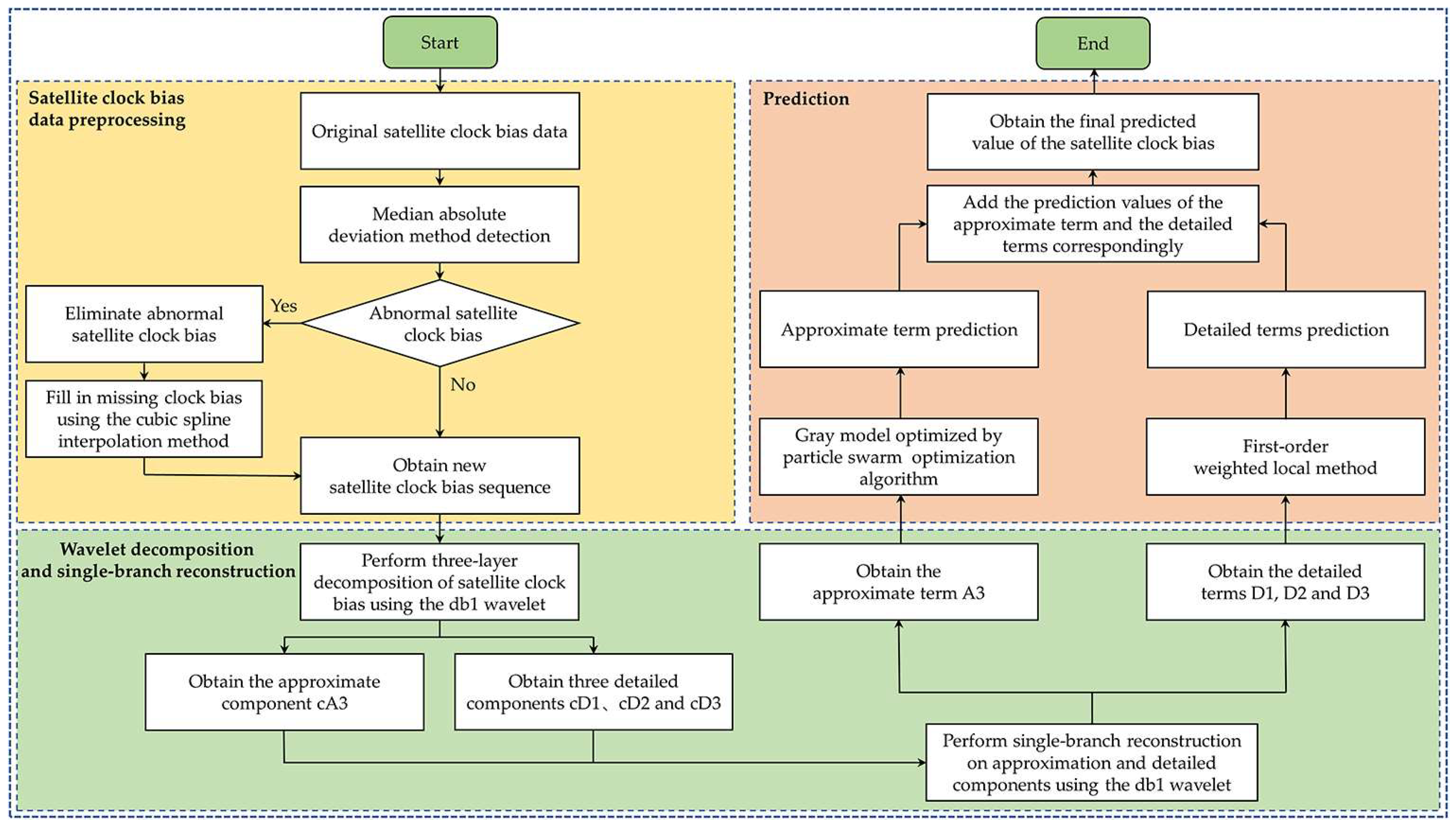
According to the features of the wavelet function and the nonlinear SCB, an appropriate wavelet function is selected to decompose and reconstruct the SCB. The SCB undergoes a three-level multi-resolution decomposition and single-branch reconstruction using the wavelet as follows:

$$SCB={\displaystyle \sum _{i=1}^3{D}_i}+A_3$$

(28)

where $SCB$ is the clock bias sequence after wavelet single-branch reconstruction; $A_3$ is the trend term after the single-branch reconstruction, which represents the low-frequency part of the SCB; and $D_i\left(i=1,2,3\right)$ are the three detailed terms, which represent the high-frequency part of the SCB. Since the SCB is the result of the synthesis of the deterministic part and various noises, the trend term obtained via wavelet decomposition and reconstruction represents the stable trend of the SCB. Specifically, after one-time accumulation of the trend term, it meets the requirements of the PGM model for the data exhibiting exponential variation characteristics. In contrast, the detailed terms present nonlinear variation characteristics and, after phase space reconstruction, they meet the requirement of the FWL method for the modeling data.

Subsequently, the appropriate number of SCB points is selected from the trend term after single-branch reconstruction, and the optimization-enhanced GM model is employed for modeling and prediction. Meanwhile, the detailed components are rebuilt in phase space according to the embedding dimension $m$ and the time delay $\tau$. The FWL method is then employed to model and predict the detailed terms in the phase space, thereby enhancing the predictive precision of the SCB.

Finally, the predicted value of the SCB can be acquired by summing the predicted results of each component accordingly. Thus, the integrated prediction model constructed by the PGM model and the FWL method can be expressed as:

$$SC{B}_{pre}=T_{PGM}+{\displaystyle \sum _{i=1}^3{f}_i\left(m,\tau \right)T_i}$$

(29)

where $T_{PGM}$ denotes the predicted value from the PGM model for the trend term $A_3$; $T_i$ denotes the predicted value of the detailed terms $D_i\left(i=1,2,3\right)$ using the FWL method; $f_i\left(m,\tau \right)$ is the fitting factor, and the change of any parameter $m$ and $\tau$ affects the fitting precision of the prediction value $T_i$; and $SC{B}_{pre}$ is the ultimate predicted SCB from the integrated model. The detailed procedures are outlined below:

(1)

SCB preprocessing. Owing to the frequent jumps in SCB, these data are severely unfavorable for the establishment of the model. Therefore, it is very important to check the quality of SCB before modeling. In the work, the MAD method with good tolerance and timeliness is adopted for gross errors and clock jump detection. After detecting the clock jumps or gross errors, they are excluded, and then the cubic spline interpolation method is employed to make up for the missing data.

(2)

SCB decomposition and reconstruction. The SCB is essentially a time series signal, and its phase information directly affects the accuracy of the subsequent SCB prediction. Moreover, the phase distortion will cause the physical meaning of approximate terms and detailed terms to deviate from reality. The db1 wavelet is the only wavelet with a strict linear phase in the Daubechies wavelet family. It can ensure that the phase delay of each component is strictly linear with the frequency in the process of three-layer decomposition and single-branch reconstruction. This fundamentally eliminates waveform distortion, ensuring the reliability of subsequent prediction. In this study, the db1 wavelet is used to perform three-level multi-resolution decomposition on the SCB to acquire the approximate component cA3 and three detailed components cD1, cD2, and cD3. Subsequently, the single-branch reconstruction of these components is performed to obtain the trend term A3 and the three detailed terms D1, D2, and D3. Because the db1 wavelet has symmetrical characteristics for the single-branch reconstruction of the signal, the trend term of the SCB decomposition shows a certain variation law after reconstruction, which meets the requirements of the PGM model for the modeling data. Meanwhile, the db1 wavelet has excellent linear phase characteristics, which makes it possible to decompose and reconstruct the signal without phase distortion.

(3)

Predict each component of SCB. The PGM model and the FWL method are adopted to predict the wavelet decomposed and reconstructed sequences, respectively. The trend term A3 is predicted using the PGM model; the three detailed terms D1, D2, and D3 are predicted using the FWL method.

(4)

The ultimate prediction of SCB. By adding the sequence of the trend term predicted by the PGM model to the sequence of the three detailed terms predicted by the FWL method, the ultimate SCB prediction can be acquired.

Relative to the unitary prediction approaches, the integrated predictive strategies proposed herein decompose the SCB via the WT and perform single-branch reconstruction to separate it into a trend term and three detailed terms. Depending on the variation features of each component, the best prediction model is employed, respectively, for fitting and prediction. The algorithm can significantly reduce prediction errors and has higher prediction precision compared with the single prediction model.

The prediction procedure of the WT-PGM-FWL model is depicted in Figure 3.

3. Experimental Results

Since the convergence and accuracy of the PPP can be significantly improved by utilizing the SCB with a 30 s sampling interval, the SCB issued by the GNSS Data Analysis Center of WHU is employed for experiments to test the validity and possibility of the WT-PGM-FWL model. Using the SCB from the first day of BDS week 971 as an example, only the SCB of the IGSO and MEO satellites is studied, as the majority of GNSS Data Analysis Centers at present are unable to provide ephemeris data of the GEO satellites [27]. The BDS-3 IGSO and MEO satellites are equipped with three types of clocks: hydrogen clocks for IGSO and MEO satellites and rubidium clocks for MEO satellites. In

Table 1. Types of satellite clocks in orbit BDS-3 ¹.

Orbits	PRN and Clock Types
IGSO (3)	38 (H) 39 (H) 40 (H)
MEO (24)	19 (Rb) 20 (Rb) 21 (Rb) 22 (Rb) 23 (Rb) 24 (Rb) 25 (H) 26 (H) 27 (H) 28 (H) 29 (H) 30 (H) 32 (Rb) 33 (Rb) 34 (H) 35 (H) 36 (Rb) 37 (Rb) 41 (Rb) 42 (Rb) 43 (H) 44 (H) 45 (H) 46 (H)
GEO (3)	59 (H) 60 (H) 61 (H)

¹ retrieved from http://www.igmas.org/Gnss/Xzztpg/sattable/cate_id/76.html, accessed on 1 July 2025. The bolded satellite number and clock are the ones selected for this experiment.

, the chosen satellites are highlighted in bold, covering the three kinds of clocks. Taking the corresponding SCB issued by the GNSS Data Analysis Center at WHU as the benchmark, the predicted SCB is compared against this baseline.

The RMS and the absolute value of the difference between the maximum and minimum errors, the range difference, abbreviated as Range, are adopted as the statistical quantities to evaluate the prediction results for comparing and analyzing the precision and stability of each model. Their calculation formulas are as follows:

$$RMS=\sqrt{{\displaystyle \frac{{\displaystyle \sum _{i=1}^n{\left(erro{r}^{\left(i\right)}\right)}^2}}{n}}}$$

(30)

$$Range=\left|erro{r}_{\max }^{\left(i\right)}-erro{r}_{\min }^{\left(i\right)}\right|$$

(31)

where $erro{r}^{\left(i\right)}={\widehat{x}}_i-x_i,\left(i=1,2,\cdots ,n\right)$ denotes the prediction residuals of each model; ${\widehat{x}}_i$ is the SCB predicted by each model at time $i$; $x_i$ is the SCB issued by the analysis center at time $i$; $n$ represents the count of SCB epochs; and $erro{r}_{\max }^{\left(i\right)}$ and $erro{r}_{\min }^{\left(i\right)}$ are the maximum and minimum errors in the predictive errors of each model, respectively.

3.1. Modeling with 18 H Data to Predict Satellite Clock Bias of the Next 10 Min

To assess and compare the predictive capability of the GM model and the WT-PGM-FWL model, the SCB from the first day’s 18 h (2160 epochs) was chosen as the modeling data. The GM model was directly applied to the preprocessed SCB of the day’s first 18 h to predict the SCB over the subsequent 10 min. Moreover, the WT-PGM-FWL model first used the db1 wavelet to perform three-level multi-resolution decomposition on the preprocessed SCB and then performed single-branch reconstruction on the decomposed components. Due to space limitations, only the wavelet decomposition and single-branch reconstruction diagrams for the C38 satellite are presented, as shown in Figure 4.

As observed in Figure 4a, the SCB is decomposed by the three levels of the db1 wavelet, and one trend component and three detailed components are obtained. The number of points of the sequence after each level of decomposition is half of that of the previous level. The trend component shows an approximate linear changing trend, while the three detailed components show irregular nonlinear characteristics. To ensure the consistency of the dimensions, single-branch reconstruction is performed on both the trend component and the three detailed components. From Figure 4b, after the trend component and the three detailed components are processed by the single-branch reconstruction, the number of data points of each component is the same as that of the raw SCB. This property ensures the completeness of the reconstructed data in the time dimension, which provides a necessary prerequisite for the dimensional alignment and the joint analysis in the subsequent multi-component modeling. Moreover, the db1 wavelet exhibits a unique linear phase property during the signal reconstruction process. This property implies that the phase delay of each frequency component of the signal maintains a strictly linear relationship with its frequency during the decomposition and reconstruction processes. Consequently, the waveform distortion problem caused by nonlinear phase distortion is fundamentally eliminated. For the approximate term A3 after single-branch reconstruction, the PGM model is employed for modeling and predicting. Meanwhile, for the single-branch reconstructed detailed terms D1, D2, and D3, the FWL method is employed for modeling and predicting. Then, the prediction results of the two models are summed correspondingly to obtain the prediction results of the WT-PGM-FWL model, i.e., the SCB’s final prediction. Eventually, the predictive errors of the novel model are obtained by subtracting its prediction results from the SCB published by the GNSS Data Analysis Center of WHU, and these results are subsequently contrasted with those derived from the standalone GM model to assess performance improvements. Owing to space limitations, only the prediction errors for the C23, C25, and C38 satellites are presented, as shown in Figure 5. The statistics of RMS and range are listed in

Table 2. Statistics of prediction precision RMS of the GM model and the WT-PGM-FWL model for various types of satellite clocks (18 h modeling and 10 min predicting) (Unit: ns).

Model	RMS
	MEO Rb				IGSO H		MEO H		All	Deviation Range
	C23	C33	C36	C37	C38	C40	C25	C43
GM	0.33	0.10	0.23	0.29	0.10	0.23	0.57	0.07	0.24	0.50
WT-PGM-FWL	0.04	0.04	0.17	0.02	0.03	0.07	0.05	0.02	0.06	0.15

“All” represents the average values of all the satellites’ prediction precision RMS.

and

Table 3. Statistics of prediction stability range of the GM model and the WT-PGM-FWL model for various types of satellite clocks (18 h modeling and 10 min predicting) (Unit: ns).

Model	Range
	MEO Rb				IGSO H		MEO H		All	Deviation Range
	C23	C33	C36	C37	C38	C40	C25	C43
GM	0.05	0.06	0.05	0.06	0.05	0.06	0.09	0.06	0.06	0.04
WT-PGM-FWL	0.03	0.04	0.03	0.05	0.03	0.05	0.06	0.04	0.04	0.03

“All” represents the average values of all the satellites’ prediction stability range.

.

From Figure 5, for the MEO-Rb C23, the MEO-H C25, and the IGSO-H C38 satellites, the prediction error of the WT-PGM-FWL model fluctuates slightly near zero, and the accumulation speed of the errors is relatively slow over time, especially for the IGSO-H C38 satellite, where the error fluctuation range remains within 0.06 ns. Additionally, its predictive results are steadier when compared to those of the standalone GM model, with the predicted SCB being closer to the actual values, showing that the WT-PGM-FWL model possesses superior prediction precision and performance. In contrast, the error of the standalone GM model is farther away from zero, with the maximum error fluctuation range reaching 0.60 ns, and the accumulation rate of the errors is relatively fast with the increase in predicting time. Moreover, the GM model exhibits roughly similar errors for different satellites. The error for the C23 MEO-Rb ranges from −0.40 to −0.30 ns, for the C25 MEO-H from −0.60 to −0.40 ns, and for the C38 IGSO-H from −0.12 ns to −0.08 ns. The GM model exhibits roughly similar errors towards different satellites from two factors: First, the GM model assumes that the cumulative SCB sequence follows a first-order linear differential equation, but the actual SCB has the characteristics of being non-stationary and nonlinear, resulting in inherent fitting errors during the accumulation process. Second, the LS method used for GM parameter estimation is prone to falling into a local optimum, amplifying the initial fitting error. At the 0 min point, the GM error is a fitting residual rather than a prediction error.

From Table 2 and Table 3, on the whole, the prediction precision and stability of the WT-PGM-FWL model are significantly higher than those of the standalone GM model for various types of clocks. The mean prediction precision and stability of the novel model stand at 0.06 ns and 0.04 ns, while the standalone GM model exhibits 0.24 ns and 0.06 ns for these metrics, respectively. In comparison to the standalone GM model, the proposed model’s mean prediction precision and stability show improvements of 75.00% and 33.33%, respectively. Additionally, when compared to the WT-PGM-FWL model, the mean value and the deviation range of the RMS and range of the standalone GM model are relatively large, especially the mean value and the deviation range of the prediction precision RMS, which reach 0.24 ns and 0.50 ns.

3.2. Modeling with 18 H Data to Predict Satellite Clock Bias of the Next 30 Min and 60 Min

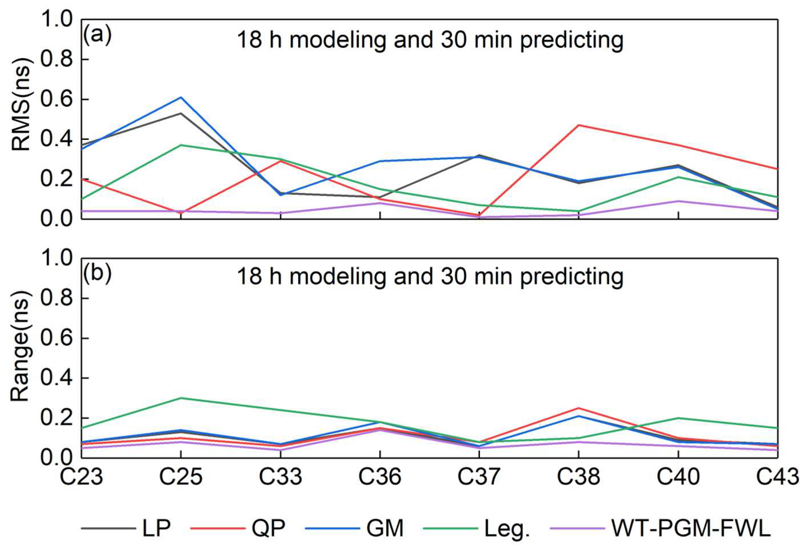
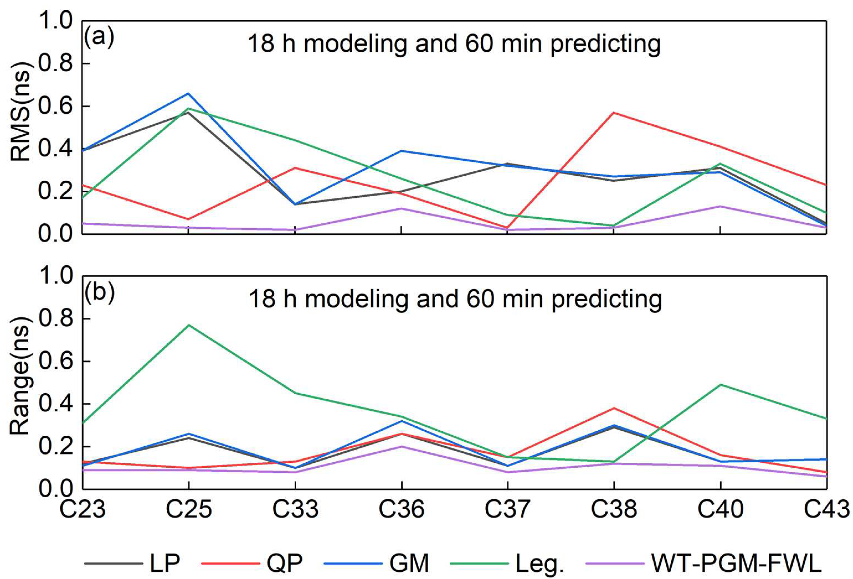
For a comprehensive validation and analysis of the workability and efficacy of the WT-PGM-FWL model, the SCB of the day’s first 18 h (2160 epochs) are adopted as modeling inputs, and the LP, QP, GM, Leg. polynomial, and WT-PGM-FWL models are established, respectively, to generate SCB prediction for the subsequent 30 min and 60 min. Figure 6 and Figure 8 present the variations in prediction precision RMS and stability range of the five models for various types of clocks under various prediction periods, respectively. The variation in the bar charts of prediction precision and stability for various types of clocks with various prediction durations for the five models is given in Figure 7 and Figure 9. The statistics of prediction precision and stability of the five models for various types of satellite clocks at various prediction durations are given in

Table 4. Statistics of prediction precision RMS of the five models for various types of satellite clocks (18 h modeling, 30 min and 60 min predicting) (Unit: ns).

Clock Type	RMS
	18 H Modeling and 30 Min Predicting					18 H Modeling and 60 Min Predicting
	LP	QP	GM	Leg.	WT-PGM-FWL	LP	QP	GM	Leg.	WT-PGM-FWL
MEO-Rb	0.23	0.15	0.27	0.16	0.04	0.27	0.19	0.31	0.24	0.05
MEO-H	0.30	0.14	0.33	0.24	0.04	0.31	0.15	0.35	0.35	0.06
IGSO-H	0.23	0.42	0.23	0.13	0.06	0.28	0.49	0.28	0.19	0.08
All	0.25	0.24	0.28	0.18	0.05	0.29	0.28	0.31	0.26	0.06

“All” represents the average values of all the satellites’ prediction precision RMS.

and Table 6, respectively.

Table 5. Average precision of the predicted SCB products of the five models for various types of satellite clocks (18 h modeling, 30 min and 60 min predicting) (Unit: ns).

Clock Type	RMS
	18 H Modeling and 30 Min Predicting					18 H Modeling and 60 Min Predicting
	LP	QP	GM	Leg.	WT-PGM-FWL	LP	QP	GM	Leg.	WT-PGM-FWL
MEO-Rb	0.38	0.30	0.42	0.31	0.19	0.42	0.34	0.46	0.39	0.20
MEO-H	0.45	0.29	0.48	0.39	0.19	0.46	0.30	0.50	0.50	0.21
IGSO-H	0.38	0.47	0.38	0.28	0.21	0.43	0.64	0.43	0.34	0.23
All	0.40	0.35	0.43	0.33	0.20	0.44	0.43	0.46	0.41	0.21

“All” represents the average values of all the satellites’ prediction precision RMS.

displays the mean precision of the predicted SCB products in accordance with multiple sorts of clocks and diverse periods.

It can be concluded from Figure 6, Figure 7, Figure 8 and Figure 9 and Table 4, Table 5 and

Table 6. Statistics of prediction stability range of the five models for various types of satellite clocks (18 h modeling, 30 min and 60 min predicting) (Unit: ns).

Clock Type	Range
	18 H Modeling and 30 Min Predicting					18 H Modeling and 60 Min Predicting
	LP	QP	GM	Leg.	WT-PGM-FWL	LP	QP	GM	Leg.	WT-PGM-FWL
MEO-Rb	0.09	0.09	0.10	0.16	0.07	0.15	0.17	0.16	0.31	0.11
MEO-H	0.10	0.08	0.11	0.23	0.06	0.19	0.09	0.20	0.55	0.08
IGSO-H	0.15	0.18	0.15	0.15	0.07	0.21	0.27	0.22	0.31	0.12
All	0.11	0.12	0.12	0.18	0.07	0.18	0.18	0.19	0.39	0.10

“All” represents the average values of all the satellites’ prediction stability range.

that the WT-PGM-FWL model significantly exceeds several other traditional models in both prediction precision and stability for the two prediction durations across diverse types of satellite clocks. Especially for the IGSO C40 satellite, the other four models exhibit far lower prediction precision and stability compared to the WT-PGM-FWL model, as depicted in Figure 6 and Figure 8. The statistics of mean prediction outcomes derived from diverse clock types with different prediction durations were calculated, and the corresponding RMS as well as range are presented in Table 4 and Table 6. Based on the statistical averages of prediction results for diverse types of clocks, Figure 7 and Figure 9 present the bar graphs of the prediction precision RMS and stability range for various clock types across two prediction durations.

It is clear from Table 4 and Table 6 that the WT-PGM-FWL model exhibits better prediction precision and stability than the other four models, across the two prediction durations, when considering diverse satellite clock types. For 30 min prediction durations, the mean predictive precision and stability of these four models are (0.25, 0.24, 0.28, and 0.18) ns and (0.11, 0.12, 0.12, and 0.18) ns, whereas those of the WT-PGM-FWL model are 0.05 ns and 0.07 ns, respectively. Relative to the other four models, the WT-PGM-FWL model exhibits superior mean precision and robustness, with precision increasing by (80.00, 79.16, 82.14, and 72.22) % and stability by (36.36, 41.67, 41.67, and 61.11) %, respectively. For 60 min prediction durations, these four models exhibit mean prediction precisions of (0.29, 0.28, 0.31, and 0.26) ns, along with stability of (0.18, 0.18, 0.19, and 0.39) ns, respectively. In contrast, the WT-PGM-FWL model achieves a superior mean prediction precision of 0.05 ns and better mean stability of 0.07 ns, demonstrating improvements by (79.31, 78.57, 80.65, and 76.92) % in precision and (44.44, 44.44, 47.37, and 74.36) % in stability relative to the four comparison models. It is also found that, under the same modeling conditions, the prediction precision and stability of the four models decrease along with the rise in prediction spans, especially the Leg. polynomial model, which has the fastest decrease in prediction precision and stability. However, the WT-PGM-FWL model does not exhibit such an obvious phenomenon, and its changes are very slight. This indicates that, to some extent, the WT-PGM-FWL model can alleviate the problem that the prediction precision and stability decrease rapidly with the prolongation of prediction time. For multiple satellite clock categories and prediction timescales, Table 5 quantifies the mean precision of the predicted SCB products. For the predicted SCB products, their RMS equals the arithmetic sum of the RMS of the precise ephemeris in real-time service (RTS) products and the RMS derived from SCB prediction, with the ultimate precise ephemeris precision of RTS products being 0.15 ns.

It is evident from Table 5 that the mean precision of the SCB products predicted by the four models fails to satisfy the precision demands of a threshold of under 0.30 ns during the two prediction periods. For the WT-PGM-FWL model, the prediction precision of SCB products remains superior to 0.21 ns in 30 min and 60 min. To be specific, this model demonstrates prediction precision exceeding 0.30 ns for all satellite clock types, where a precision of 0.30 ns gives rise to a ranging error of roughly 0.09 m. Additionally, the mean precision of the SCB products from the WT-PGM-FWL model exhibits improvements by (50.00, 42.86, 53.49, and 39.40) % for 30 min and (52.27, 51.16, 54.35, and 48.78) % for 60 min relative to the other four models, respectively. Therefore, the SCB predicted products of the WT-PGM-FWL model can temporarily replace RTS products during outages, thereby satisfying the centimeter-level positioning precision requirement for RT-PPP over 60 min.

3.3. Modeling with 20 H Data to Predict Satellite Clock Bias of the Next 60 Min

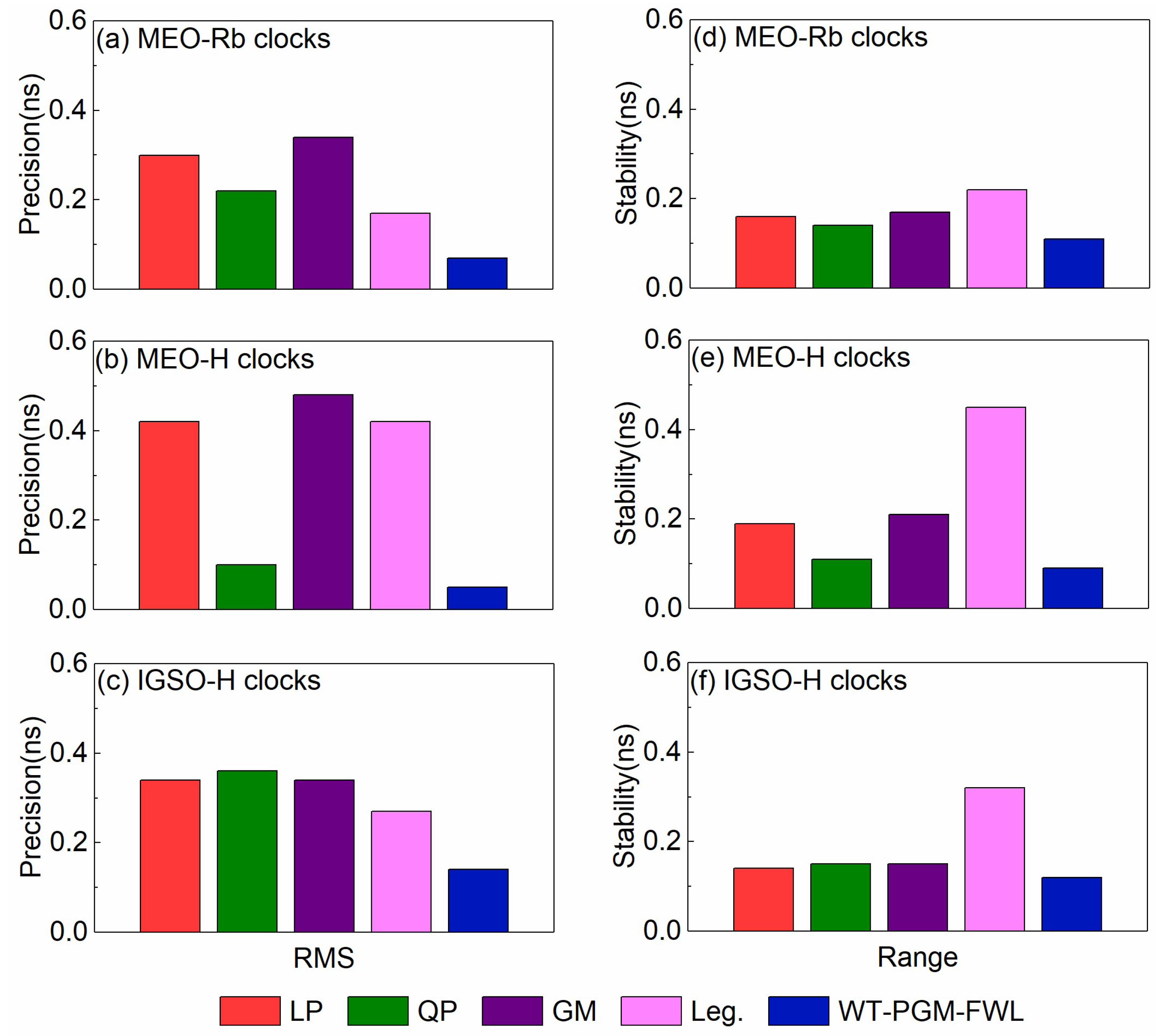
For a deeper analysis of the prediction capability of the WT-PGM-FWL model under various modeling duration conditions, the analysis is performed by increasing the length of the modeling data. Using the SCB from the day’s first 20 h (2400 epochs) as the modeling data, the LP, QP, GM, Leg. polynomial, and WT-PGM-FWL models are constructed in turn to predict the SCB over the subsequent 60 min. Figure 10 illustrates the variation in prediction precision and stability for the five models across various clock types. Figure 11 shows the prediction precision and stability bar charts for various types of clocks. The statistics of prediction precision and stability of the five models for various kinds of clocks are tabulated in

Table 7. Statistics of prediction precision RMS and stability range of the five models for various types of satellite clocks (20 h modeling and 60 min predicting) (Unit: ns).

Clock Type	20 H Modeling and 60 Min Predicting
	RMS					Range
	LP	QP	GM	Leg.	WT-PGM-FWL	LP	QP	GM	Leg.	WT-PGM-FWL
MEO-Rb	0.30	0.22	0.34	0.17	0.07	0.16	0.14	0.17	0.22	0.11
MEO-H	0.42	0.10	0.48	0.42	0.05	0.19	0.11	0.21	0.45	0.09
IGSO-H	0.34	0.36	0.34	0.27	0.14	0.14	0.15	0.15	0.32	0.12
All	0.35	0.23	0.39	0.29	0.09	0.16	0.13	0.18	0.33	0.11

“All” represents the average values of all the satellites’ prediction precision RMS or stability range.

. The mean precision of the predicted SCB products of the five models for diverse kinds of clocks is documented in Table 4.

From Figure 10, for different types of satellite clocks, the WT-PGM-FWL model performs better than the other four models with regard to both prediction precision and stability. When it comes to prediction precision, the C25 satellite shows poor performance. For this satellite, the prediction precision of the GM model is close to 1.00 ns, followed by the LP model, which is close to 0.80 ns, and then the Leg. polynomial model, which is close to 0.60 ns. Additionally, the QP model’s prediction precision is on a par with the WT-PGM-FWL model for the C25 satellite, but the WT-PGM-FWL model is marginally superior to the QP model in this regard. With regard to prediction stability, the C25 satellite also demonstrates relatively lower prediction stability. For this satellite, the prediction stability of the Leg. polynomial model exceeds 0.60 ns. Prediction stability for the GM and LP models is similar, nearing 0.30 ns, with the LP model outperforming the GM model by a small margin. Furthermore, the prediction stability of the QP model and the WT-PGM-FWL model is basically the same; they are both less than 0.20 ns. Nevertheless, the WT-PGM-FWL model achieves markedly superior stability compared to the QP model. In light of the statistical information concerning mean prediction outcomes across diverse clock types, the bar charts showing the prediction precision RMS and stability range within a 60 min prediction period are depicted in Figure 11. The relevant prediction precision RMS and stability range versus the predicted SCB products of the five models are tabulated in Table 7 and

Table 8. Average precision of the predicted SCB products of the five models for various types of satellite clocks (20 h modeling and 60 min predicting) (Unit: ns).

Clock Type	20 H Modeling and 60 Min Predicting
	RMS
	LP	QP	GM	Leg.	WT-PGM-FWL
MEO-Rb	0.45	0.37	0.49	0.32	0.22
MEO-H	0.57	0.25	0.63	0.57	0.20
IGSO-H	0.49	0.55	0.49	0.42	0.29
All	0.50	1.17	0.54	0.44	0.24

“All” represents the average values of all the satellites’ prediction precision RMS.

.

Table 7 illustrates that the mean prediction precision and stability of the GM model rank the poorest; in contrast, those of the WT-PGM-FWL model surpass those of the other four models. The WT-PGM-FWL model achieves a mean prediction precision of 0.09 ns and stability of 0.11 ns, representing improvements by (72.29, 60.87, 76.92, and 68.97) % in prediction precision and improvements by (31.25, 15.38, 38.89, and 66.67) % in prediction stability compared with those of the other four models, respectively. Furthermore, Table 8 shows that the mean precision of the predicted SCB products from several other conventional models fails to satisfy the precision specification of less than 0.30 ns. Of these models, the QP model’s mean prediction precision ranks the lowest, with a value of 1.17 ns. Such an SCB precision will result in a ranging error of 0.35 m, which is insufficient for the requirement of centimeter-level positioning. In contrast, the WT-PGM-FWL model achieves a predictive precision of better than 0.24 ns for diverse types of clocks. Moreover, a prediction precision of 0.24 ns will bring about a ranging error of 7.20 cm, which is capable of satisfying the specifications of the SCB precision for centimeter-level positioning.

4. Discussion

The precision of the SCB prediction is of crucial importance to GNSS service quality. According to the features of SCB, we perform a hybrid model that integrates WT, PGM, and FWL methods. It demonstrates marked superiority in the short-duration prediction of the BDS-3 SCB. In the 10 min prediction, the novel model achieved remarkable prediction performance. In contrast, the MEO-H satellites have the highest mean prediction precision and stability of 0.04 ns and 0.05 ns, respectively. Since the SCB characteristics of different types vary significantly, the traditional GM model employs a uniform LS method to estimate its parameters, which tends to easily reach the local optimum and is unable to adaptively adjust the parameters for different types of clocks. As a result, its mean prediction precisions and stabilities for the MEO-Rb, IGSO-H, and MEO-H satellites are poor, reaching (0.24, 0.17, and 0.32) ns and (0.06, 0.06, and 0.08) ns, respectively. Compared to the traditional GM model, the WT-PGM-FWL model improves the mean prediction precision and stability by (70.83, 70.56, and 87.50) % and (33.33, 33.33, and 37.50) % for the same satellites, respectively. The above results demonstrate that the WT-PGM-FWL model displays superior predictive precision and stability with respect to various types of clocks.

During the 30 min and 60 min predictions, the WT-PGM-FWL model is more capable of reflecting the changing trend of the SCB. Relative to the remaining four models, the WT-PGM-FWL model’s mean prediction precision and stability can achieve improvements of up to around 82.14% and 74.36%, respectively. Under the same modeling conditions, as prediction duration is extended, the bar charts in Figure 7 and Figure 9 illustrating mean prediction precision and stability for diverse types of clocks make it clear that all five models display a phenomenon where prediction performance degrades along with the rise in prediction duration. Nevertheless, in terms of the values for mean prediction precision and stability, as presented in Table 4 and Table 6, the variation range of the WT-PGM-FWL model’s predicted results is prominently lower than those of several other conventional models; concerning prediction results across diverse clock types, the four conventional models demonstrate better prediction performance for rubidium clocks compared to hydrogen clocks. However, the values of precision and stability predicted by the WT-PGM-FWL model for these two types of clocks do not change much. This indicates that the novel model will not be affected by the types of clocks, and it has a better prediction ability for the SCB of diverse types of clocks.

Comparison of Table 4, Table 5, Table 6, Table 7 and Table 8 shows that, on the whole, with the increase in the quantity of modeling data, most of the prediction precision and stability of the four conventional models slightly decrease, while most of those of the QP model slightly increase. This indicates that more data involved in modeling is not always better. However, for the WT-PGM-FWL model, both prediction precision and stability show little variation as the quantity of modeling data increases, without any sharp decline or rise. There exist three primary causes why the WT-PGM-FWL model can achieve higher SCB prediction outcomes than several other traditional models. The first cause lies in the time–frequency properties of wavelet decomposition; the SCB is decomposed and reconstructed into a low-frequency trend term and three high-frequency detailed terms using the db1 wavelet. Wavelet threshold denoising can effectively filter out random noise in each component. The trend term is predicted by the PGM model, which captures the long-term evolution patterns, while the three detailed terms are predicted after characterizing the nonlinear fluctuations using the FWL method, realizing targeted modeling and prediction. The second cause is the global optimization of the GM model by the PSO. Since the parameter estimation of the traditional GM model employs the LS method, it is prone to falling into a local optimum. By introducing the PSO to conduct a global search for the two parameters of the GM model, its prediction ability can be enhanced. The third cause is the high-frequency adaptability of the FWL method. The SCB is essentially a nonlinear chaotic sequence whose neighboring points in its phase space have similar evolutionary trajectories. The FWL method uses phase space reconstruction to find the nearest points of the current state and employs a local linear approximation to establish a model for the detailed terms. This approach can accurately capture the characteristics of chaotic systems, thereby enabling high-precision predictions.

5. Conclusions

To boost the precision and stability of the single model in SCB prediction, a hybrid model is proposed by integrating the WT, the PGM model, and the FWL method. The novel model utilizes the db1 wavelet to perform three-level multi-scale decomposition and single-branch reconstruction on the SCB, obtaining an approximation term and three detailed terms. According to the variation characteristics of each component, a suitable prediction model is constructed. Among them, the approximate term is predicted by the PGM model, and the three detailed terms are predicted by the FWL method. Ultimately, the SCB’s final prediction is acquired by summing the prediction outcomes of each component. Through experiments and analysis, the reliability and effectiveness of the WT-PGM-FWL model for nonlinear SCB prediction are demonstrated. This model not only improves the precision and stability of the single SCB predicting model but also reduces their prediction risks. The main conclusions are summarized as follows:

(1)

Due to the high-frequency sensitivity of satellite atomic clocks, they are highly susceptible to complex space environmental factors, causing the output SCB to exhibit non-stationary and nonlinear trends. A single prediction model has certain limitations on SCB prediction and shows significant differences in predicting diverse types of clocks.

(2)

The WT-PGM-FWL model exhibits remarkable advantages in the precision and stability of SCB prediction, and its performance markedly exceeds that of several other models. Additionally, as the prediction time becomes longer, the WT-PGM-FWL model exhibits excellent robustness properties. The rate of error growth is significantly lower than that of other comparison models, and it can also maintain high prediction precision and stability.

(3)

The predictive precision and stability of the WT-PGM-FWL model for the SCB of hydrogen clocks are the same as those of rubidium clocks. It is not affected by the types of clocks and demonstrates good prediction ability for the SCB of diverse types of clocks. Furthermore, as the amount of modeling data increases, its prediction precision and stability exhibit little variation, and there is no phenomenon where the prediction precision and stability significantly decrease or increase.

(4)

For 30 min and 60 min predictions, the precision of the SCB products from the WT-PGM-FWL model all fall below 0.30 ns. Therefore, when users have poor communication and cannot obtain the RTS products, the SCB within a 1 h duration predicted by the WT-PGM-FWL model can be used in place of the RTS products, thereby guaranteeing the precision of RT-PPP over the 1 h period of communication interruption.

References

1. Yang, Y.; Yao, Z.; Mao, Y.; Xu, T.; Wang, D. Resilient satellite-based PNT system design and key technologies. Sci. China Ser. D-Earth Sci. 2025, 68, 669–682. [Google Scholar] [CrossRef]
2. Geng, J.; Wen, Q.; Chen, G.; Dumitraschkewitz, P.; Zhang, Q. All-frequency IGS phase clock/bias product combination to improve PPP ambiguity resolution. J. Geod. 2024, 98, 48. [Google Scholar] [CrossRef]
3. Ahmed, E.M.; Manoj, D. Maintaining real-time precise point positioning during outages of orbit and clock corrections. GPS Solut. 2016, 21, 937–947. [Google Scholar]
4. Wang, X.; Chai, H.; Wang, C. A high-precision short-term prediction method with stable performance for satellite clock bias. GPS Solut. 2020, 24, 105–115. [Google Scholar] [CrossRef]
5. Huang, B.; Ji, Z.; Zhai, R.; Xiao, C.; Wang, Y. Clock bias prediction algorithm for navigation satellites based on a supervised learning long short-term memory neural network. GPS Solut. 2021, 25, 80. [Google Scholar] [CrossRef]
6. Zhao, L.; Na, Z.; Li, L.; Cui, P. SSA-TCN: Satellite clock offset prediction during outages of RTS stream. GPS Solut. 2025, 29, 105–121. [Google Scholar] [CrossRef]
7. Elsobeiey, M.; Al-Harbi, S. Performance of real-time Precise Point Positioning using IGS real-time service. GPS Solut. 2016, 20, 565–571. [Google Scholar] [CrossRef]
8. Jaduszliwer, B.; Camparo, J. Past, present and future of atomic clocks for GNSS. GPS Solut. 2021, 25, 27. [Google Scholar] [CrossRef]
9. Jin, S.; Su, K. PPP models and performances from single- to quad-frequency BDS observations. Satell. Navig. 2020, 1, 16. [Google Scholar] [CrossRef]
10. Zhang, B.; Chen, Y.; Yuan, Y. PPP-RTK based on undifferenced and uncombined observations: Theoretical and practical aspects. J. Geod. 2019, 93, 1011–1024. [Google Scholar] [CrossRef]
11. Li, B.; Ge, H.; Bu, Y.; Zheng, Y.; Yuan, L. Comprehensive assessment of real-time precise products from IGS analysis centers. Satell. Navig. 2022, 3, 12. [Google Scholar] [CrossRef]
12. Hadas, T.; Bosy, J. IGS RTS precise orbits and clocks verification and quality degradation over time. GPS Solut. 2015, 19, 93–105. [Google Scholar] [CrossRef]
13. Hu, C.; Wang, Q. BDS-3/GNSS satellite ultra-rapid clock offsets estimation model with the aid of onboard clock states Solution. Acta Geod. Cartogr. Sin. 2024, 53, 2268–2281. [Google Scholar]
14. Yan, X.; Li, W.; Yang, Y.; Li, W.; Yang, Y.; Pan, X. BDS satellite clock prediction based on a semiparametric adjustment model considering model errors. Satell. Navig. 2020, 1, 11. [Google Scholar] [CrossRef]
15. Hu, C.; Wang, Q.; Min, Y.; Mao, Y.; Gong, Y. An improved model for BDS satellite ultra-rapid clock offsets prediction based on BDS-2 and BDS-3 combined estimation. Acta. Geod. Geophys. 2019, 54, 513–543. [Google Scholar] [CrossRef]
16. Nie, Z.; Gao, Y.; Wang, Z.; Ji, S.; Yang, H. An approach to GPS clock prediction for real-time PPP during outages of RTS stream. GPS Solut. 2018, 22, 14. [Google Scholar] [CrossRef]
17. Guo, J.; Xu, X.; Zhao, Q.; Liu, J. Precise orbit determination for quad-constellation satellites at Wuhan University: Strategy, result validation, and comparison. J. Geod. 2016, 90, 143–159. [Google Scholar] [CrossRef]
18. Huang, G.; Cui, B.; Zhang, Q.; Fu, W.; Li, P. An Improved Predicted Model for BDS Ultra-Rapid Satellite Clock Offsets. Remote Sens. 2018, 10, 60. [Google Scholar] [CrossRef]
19. Ye, S.; Zhao, L.; Song, J.; Chen, D.; Jiang, W. Analysis of estimated satellite clock biases and their effects on precise point positioning. GPS Solut. 2018, 22, 16. [Google Scholar] [CrossRef]
20. Lv, K.; Cai, C.; Cai, Y.; Guan, W.; Fang, Y. Highly accurate short-term prediction of BDS-3 satellite clock bias based on SSA-ANFIS integrated modeling. GPS Solut. 2025, 29, 100–112. [Google Scholar] [CrossRef]
21. Tu, R.; Zhang, P.; Zhang, R.; Liu, J.; Lu, X. Modeling and performance analysis of precise time transfer based on BDS triple-frequency un-combined observations. J. Geod. 2019, 93, 837–847. [Google Scholar] [CrossRef]
22. Ai, Q.; Xu, T.; Sun, D.; Ren, L. The Prediction of BeiDou Satellite Clock Bias Based on Periodic Term and Starting Point Deviation Correction. Acta Geod. Cartogr. Sin. 2016, 45, 132–138. [Google Scholar]
23. Huang, G. Research on Algorithms of Precise Clock Offset and Quality. Ph.D. Thesis, Chang’an University, Xi’an, China, 2012. [Google Scholar]
24. Hauschild, A.; Montenbruck, O.; Steigenberger, P. Short-term analysis of GNSS clocks. GPS Solut. 2013, 17, 295–307. [Google Scholar] [CrossRef]
25. Busca, G.; Wang, Q. Time prediction accuracy for a space clock. Metrologia 2003, 40, 265–269. [Google Scholar] [CrossRef]
26. Lv, D.; Liu, G.; Ou, J.; Wang, S.; Gao, M. Prediction of GPS Satellite Clock Offset Based on an Improved Particle Swarm Algorithm Optimized BP Neural Network. Remote Sens. 2022, 14, 2407. [Google Scholar] [CrossRef]
27. He, S.; Liu, J.; Zhu, X.; Dai, Z.; Li, D. Research on modeling and predicting of BDS-3 satellite clock bias using the LSTM neural network model. GPS Solut. 2023, 27, 108–119. [Google Scholar] [CrossRef]
28. Huang, F.; Chen, Y.; Li, T.; Yuan, H.; Shan, Q. A Satellite Clock Bias Prediction Algorithm Based on Grey Model and Chaotic Time Series. Acta Electron. Sin. 2019, 47, 1416–1424. [Google Scholar]
29. Sun, W.; Chen, J.; Hu, C.; Lin, Y.; Wang, M.; Zhao, H.; Zhao, R.; Fu, G.; Zhao, T. Clock bias prediction of navigation satellite based on BWO-CNN-BiGRU-attention model. GPS Solut. 2025, 29, 46–59. [Google Scholar] [CrossRef]
30. Molaei, S.; Sabaei, M.; Taheri, J. MRM-PSO: An enhanced particle swarm optimization technique for resource management in highly dynamic edge computing environments. Ad Hoc Netw. 2025, 178, 103952. [Google Scholar] [CrossRef]
31. Liu, X.; Zhu, T.; Wei, Z.; Cai, S.; Long, R.; Liu, Z. Performance analysis of a novel solar-to-hydrogen system with energy storage via machine learning and particle swarm optimization. Energy 2025, 315, 134380. [Google Scholar] [CrossRef]
32. Allaoui, M.; Belhaouari, B.; Hedjam, R.; Bouanane, K.; Kherfi, M. t-SNE-PSO: Optimizing t-SNE using particle swarm optimization. Expert. Syst. Appl. 2025, 269, 126398. [Google Scholar] [CrossRef]
Figure 1. The MAD method detects abnormal data. (a) The black line represents the variation of the original clock bias data sequence for satellite C38 (BDS-3 IGSO H); The blue line represents the corresponding frequency data of the original clock bias data for satellite C38 (BDS-3 IGSO H). It is a data sequence that has not undergone gross error detection; and (b) The blue line represents the frequency data of the original frequency data for satellite C38 (BDS-3 IGSO H) processed by the MAD method. The black line represents the clock bias data sequence corresponding to the frequency data of the original frequency data for satellite C38 (BDS-3 IGSO H) processed by the MAD method.
Remotesensing 17 02888 g001
Figure 2. Flow chart of the PGM algorithm.
Remotesensing 17 02888 g002
Figure 3. Flowchart of SCB prediction integrating the PGM model and the FWL method.
Remotesensing 17 02888 g003
Figure 4. The wavelet decomposition and single-branch reconstruction of SCB for the C38 satellite. where (a) is the clock bias decomposition of satellite C38 (BDS-3 IGSO H); (b) is the clock bias reconstruction of satellite C38 (BDS-3 IGSO H).
Remotesensing 17 02888 g004
Figure 5. The error variations of the 10 min SCB prediction using the GM model and the WT-PGM-FWL model for the C23, C25, and C38 satellites, respectively.
Remotesensing 17 02888 g005
Figure 6. Prediction precision RMS and stability range of the five models for various types of satellite clocks (18 h modeling and 30 min predicting). (a) prediction accuracy; and (b) prediction stability.
Remotesensing 17 02888 g006
Figure 7. Prediction precision RMS and stability range bar chart for various types of satellite clocks (18 h modeling and 30 min predicting).
Remotesensing 17 02888 g007
Figure 8. Prediction precision RMS and stability range of the five models for various types of satellite clocks (18 h modeling and 60 min predicting). (a) prediction accuracy; and (b) prediction stability.
Remotesensing 17 02888 g008
Figure 9. Prediction precision RMS and stability range bar chart for various types of satellite clocks (18 h modeling and 60 min predicting).
Remotesensing 17 02888 g009
Figure 10. Prediction precision RMS and stability range of the five models for various types of satellite clocks (20 h modeling and 60 min predicting). (a) prediction accuracy; and (b) prediction stability.
Remotesensing 17 02888 g010
Figure 11. Prediction precision RMS and stability range bar chart for various types of satellite clocks (20 h modeling and 60 min predicting).
Remotesensing 17 02888 g011