A Selective State-Space-Model Based Model for Global Zenith Tropospheric Delay Prediction

Abstract

The Zenith Tropospheric Delay (ZTD) is a significant atmospheric error affecting the accuracy of the Global Navigation Satellite System (GNSS). Accurate estimation of the ZTD is essential for enhancing GNSS positioning precision and plays a critical role in meteorological and climate-related applications. To address the limitations of current deep learning models in capturing long-term dependencies in ZTD sequences and overcoming computational inefficiencies, this study proposes SSMB-ZTD—an efficient deep learning model based on an improved selective State Space Model (SSM) architecture. To address the challenge of modeling long-term dependencies, we introduce a joint time and position embedding mechanism, which enhances the model’s ability to learn complex temporal patterns in ZTD data. For improving efficiency, we adopt a lightweight selective SSM structure that enables linear-time modeling and fast inference for long input sequences. To assess the effectiveness of the proposed SSMB-ZTD model, this study employs high-precision Zenith Tropospheric Delay (ZTD) products obtained from 27 IGS stations as reference data. Each model is provided with 72 h of historical ZTD inputs to forecast ZTD values at lead times of 3, 6, 12, 24, 36, and 48 h. The predictive performance of the SSMB-ZTD model is evaluated against several baseline models, including RNN, LSTM, GPT-3, Transformer, and Informer. The results show that SSMB-ZTD consistently outperforms RNN, LSTM, and GPT-3 in all prediction scenarios, with average improvements in RMSE reaching 31.2%, 37.6%, and 48.9%, respectively. In addition, compared with the Transformer and Informer models based on the attention mechanism, the SSMB-ZTD model saves 47.6% and 21.2% of the training time and 38.6% and 30.0% of the prediction time on average. At the same time, the accuracy is better than the two. The experimental results demonstrate that the proposed model achieves high prediction accuracy while maintaining computational efficiency in long-term ZTD forecasting tasks. This work provides a novel and effective solution for high-precision ZTD prediction, contributing significantly to the advancement of GNSS high-precision positioning and the utilization of GNSS-based meteorological information.

1. Introduction

In high-precision Global Navigation Satellite System (GNSS) positioning, electromagnetic waves propagate through the troposphere, the lowest layer of the Earth’s atmosphere, which behaves as a non-dispersive medium and causes measurable signal delays [1,2]. These delays, commonly referred to as tropospheric delays, are typically mapped to the zenith direction using a mapping function (MF), resulting in the Zenith Tropospheric Delay (ZTD) [3,4]. In the field of GNSS positioning, the positioning error caused by ZTD can be as high as 20 m under some extreme observation conditions [5]. Therefore, obtaining accurate a priori estimates of ZTD is essential. Accurate ZTD not only significantly enhances the precision of GNSS positioning and accelerates the convergence of the solution process [6,7,8], but also supports a wide range of meteorological applications, including precipitation monitoring, weather forecasting, and typhoon tracking [9,10,11]. The prediction of high-precision ZTD thus holds both scientific significance and practical value for advancing GNSS-based high-accuracy positioning and for meteorological and climatic research.

Currently, mainstream empirical models for calculating Zenith Tropospheric Delay (ZTD) include those based on measured meteorological parameters, empirical models using reanalysis data, and models derived from numerical weather prediction. However, each of these approaches has notable limitations. Among them, regarding computational models based on measured meteorological parameters, including the Hopfield model [12], Saastamoinen model [13], Black model [14], etc., the errors of meteorological data of such models will directly affect the estimation accuracy of ZTD and are limited by the need for meteorological equipment, which often makes it challenging to obtain measured meteorological parameters. Subsequently, empirical ZTD models based on reanalysis data without meteorological equipment have been developed, such as the GPT-series models [15,16,17], the UNB-series models [18,19], etc. The spatial resolution of such models is limited, and the accuracy of the models is relatively low in regions with drastic water vapor changes, such as the coasts and the tropics. In addition, some methods based on numerical weather models (NWMs) have been developed [20,21,22], which use high-resolution meteorological data, including temperature, barometric pressure, humidity, etc., to compute the ZTD, and due to the existence of an inevitable time delay and unavoidable systematic bias in the meteorological products, this results in the ZTD calculated in this way not being able to be directly applied to the field of high-precision positioning by GNSS. However, due to the complex, nonlinear high-frequency signals and prominent long-term features such as inter-annual and seasonal characteristics of the ZTD time series [23,24,25], traditional empirical models often fail to capture the intricate and long-term dynamic behavior of ZTD accurately. As a result, the accuracy of ZTD estimation using conventional models remains limited.

With the advancement of deep learning techniques over recent decades, these methods have demonstrated remarkable success across various domains due to their strong nonlinear fitting capabilities. They are increasingly being applied to Zenith Tropospheric Delay (ZTD) prediction. Deep learning models typically utilize long sequences of historical ZTD data to learn complex nonlinear relationships and periodic patterns for predictive purposes. Representative architectures include Convolutional Neural Networks (CNNs), Recurrent Neural Networks (RNNs) and Long Short-Term Memory (LSTM) networks [26,27,28,29]. However, as the length of ZTD sequences increases, these conventional deep learning methods are prone to issues such as gradient explosion and gradient vanishing [25], which hinder the model’s ability to capture long-term dependencies and may lead to unstable or divergent prediction results. To address these limitations, researchers have explored encoder-decoder frameworks combined with attention mechanisms, which model the temporal dependencies by assessing the relevance between the current time step and specific historical ones. Among these, the Transformer [30,31] and Informer [32,33] are two representative models that have shown promise in capturing long-term patterns, and these two models also achieve very high accuracy in ZTD prediction [5]. Notably, the attention-based approach has not taken into account the efficiency of the model although the accuracy has been improved to some extent; however, the model utilizing the attention mechanism needs to traverse the entire sequence for each input and the efficiency of the model drops sharply as the length of the sequence increases [34,35], which restricts its further application in long time-series ZTD prediction.

Recently, a deep learning method called Mamba, based on selective State Space Models (SSMs), has been proposed to enable efficient modeling and prediction on long time series [36]; Mamba has the characteristics of being able to handle long-distance dependency and fast inference while being able to train in parallel and has been applied in many fields such as lithium battery life prediction and remote sensing imaging fields [37,38,39]. However, directly using a standalone Mamba block for long-sequence ZTD forecasting may lead to over-compression of historical information, which prevents the model from capturing long-term temporal patterns effectively. To address this issue, we propose a novel selective SSM-based prediction model, SSMB-ZTD, which is specifically tailored for efficient and accurate ZTD forecasting. To enhance computational efficiency, our model adopts a selective SSM structure in place of conventional attention mechanisms, thereby reducing time complexity from quadratic to linear. This allows long-range information to be efficiently compressed into a state transition vector, improving both speed and scalability without sacrificing prediction accuracy. Furthermore, to enhance the model’s capability of capturing long-term dependencies, we introduce a time and position embedding mechanism, including both ZTD sequence position embeddings and global time embeddings, which encode periodic and temporal features into the input representation. This design enriches the model’s understanding of ZTD temporal structure and significantly improves predictive performance.

To summarize, the main contributions of this paper are as follows:

(1) This paper presents the first application of the selective state space model Mamba method to long-term ZTD time-series prediction as an alternative to attention-like mechanisms. This approach significantly reduces time complexity and shortens both training and prediction time, while achieving higher accuracy compared to models such as the Transformer.

(2) To improve the model’s ability to learn long-term dependencies in ZTD time series, a temporal–positional embedding layer is introduced into the input sequence. The experimental results show that this structure can effectively improve the prediction accuracy of the model.

(3) To comprehensively evaluate the model’s accuracy and robustness, we conduct multi-dimensional analyses across different geographic regions, elevation levels, and under extreme weather conditions. Additionally, we perform comparative assessments of accuracy and efficiency against other deep learning methods under varying prediction horizons. Experimental results confirm that the proposed model consistently outperforms baseline models across different prediction window lengths, offering a novel and effective solution for high-precision ZTD forecasting.

2. Materials and Methods

To support the construction and evaluation of the proposed long-term ZTD prediction model, this study utilizes high-quality Zenith Tropospheric Delay (ZTD) datasets from 27 globally distributed International GNSS Service (IGS) stations. The selection of these stations considers geographic diversity, data continuity, and climatic representativeness to ensure robust model generalization. The GNSS-derived ZTD product is recognized as the most accurate observational dataset and serves as the primary source of model input. Additionally, ERA5 reanalysis data are used to supplement segments of missing data. This section introduces the spatial distribution of selected stations and details the two ZTD data sources adopted in this study.

2.1. Research Area

To provide a more comprehensive and integrated evaluation of the prediction performance of the proposed method under varying geographic conditions, 27 globally distributed IGS stations were selected. Among these, 9, 12, and 4 are located at low, mid, and high latitudes, respectively. The station distribution and related data can be accessed via the official IGS website (https://network.igs.org/, accessed on 10 April 2025).

In this study, we selected 27 IGS stations worldwide as the basis for model training and evaluation. The selection was based on the following criteria: (1) the availability of high-quality ZTD time-series data with minimal missing values and continuous coverage from 2019 to 2022; (2) a preference for geographical diversity, including stations from different latitudes, longitudes, altitudes, and climatic zones to improve the model’s generalization capability; (3) the need to balance computational efficiency and coverage, ensuring a manageable dataset size while preserving representativeness. These criteria ensure that the dataset supports both reliable model training and meaningful evaluation across varied environmental conditions. The distribution of these stations is shown in Figure 1.

2.2. ZTD Based on GNSS

This study uses a high-precision Zenith Tropospheric Delay (ZTD) product provided by the Crustal Dynamics Data Information System (CDDIS) platform as the core dataset. The ZTD values are derived from Global Navigation Satellite System (GNSS) observations through precise point positioning (PPP) techniques and processed under a consistent strategy across all stations. Due to their centimeter-level accuracy and global coverage, GNSS-derived ZTD products are widely recognized as one of the most reliable and direct measurements of atmospheric delay, exhibiting low temporal noise and high consistency across varying geographical conditions [40,41]. These data are publicly accessible via the CDDIS website (https://cddis.gsfc.nasa.gov/archive/gnss/products/troposphere, accessed on 20 April 2025), where ZTD solutions are typically available with a latency of 1–2 days.

We select 27 IGS stations with near-continuous time series from 2019 to 2022 to ensure data completeness and spatial representativeness. Each time series has a temporal resolution of 1 h, which enables the capture of diurnal, synoptic, and seasonal variations in tropospheric delay. These ZTD measurements serve as the primary ground-truth reference for both model training and performance evaluation.

2.3. ZTD Based on ERA5

To compensate for missing segments in the GNSS ZTD time series and ensure continuity for long-term modeling, we utilize ZTD reconstructed from the fifth-generation ECMWF reanalysis dataset, ERA5. ERA5 is a global atmospheric reanalysis produced by assimilating a wide range of observational data into a consistent forecast model and is known for its high spatiotemporal resolution and physical consistency [40].

The ERA5-derived ZTD values are calculated based on the hydrostatic and wet components of atmospheric delay, using vertical profiles of pressure, temperature, and humidity available at 37 baroclinic layers. The dataset spans from 1940 to the present and provides hourly outputs at a horizontal resolution of 0.25° × 0.25°, making it suitable for spatial interpolation over GNSS station gaps and for constructing long-term reference series [41]. The ERA5 data used in this study were obtained through the Copernicus Climate Data Store (https://cds.climate.copernicus.eu/datasets/reanalysis-era5-pressure-levels, accessed on 20 April 2025) [1].

3. Methodology

Based on the GNSS-derived and ERA5-supplemented ZTD datasets described in Section 2, this section outlines the complete methodological framework for constructing the SSMB-ZTD model. The proposed approach includes a two-stage interpolation strategy for handling missing values, a joint temporal–positional embedding mechanism to enhance feature representation, and a selective state space modeling architecture based on the Mamba framework. Furthermore, the model training strategy, including input-output design, optimization settings, and evaluation protocols, is described in detail to ensure experimental reproducibility and fairness in comparative analysis. The following subsections describe each methodological component in detail.

3.1. ZTD Data Interpolation Strategy

For time periods with missing durations shorter than 72 h, periodic least-squares fitting is performed using the empirical model defined by Equations (1) and (2), based on the inherent periodicity of the ZTD time series.

$$ZTD(t)=A_0+A_1\cos (2\pi t)+B_1\sin (2\pi t)+A_2\cos (4\pi t)+B_2\sin (4\pi t)$$

(1)

$$t={\displaystyle \frac{DOY}{365.25}}+{\displaystyle \frac{HOD}{24}}$$

(2)

where $DOY$ is the day of the year, $HOD$ is the hour of the day, $A_0$ is the average ZTD value, $(A_1,B_1)$ and $(A_2,B_2)$ are the annual and semi-annual amplitudes, respectively.

For time periods with missing lengths greater than 72 h, we calculate ZWD and ZHD by ERA5 reanalyzing the weather product and Saastamoinen model, respectively, as in Equations (3)–(7):

$$ZWD={10}^{-6}{\displaystyle \int N}ds={10}^{-6}{\displaystyle \sum _i^{n-1}(N_i+N_{i+1})}\times {\displaystyle \frac{(h_{i+1}-h_i)}{2}}$$

(3)

$$ZHD=0.0022793\times {\displaystyle \frac{\left[P_1+\left(0.05+\frac{1255}{T}\right)e_1\right]}{f(\phi ,H)}}$$

(4)

$$N=k_1\times {\displaystyle \frac{P-e}{T}}+k_2\times {\displaystyle \frac{e}{T}}+k_3\times {\displaystyle \frac{e}{T^2}}$$

(5)

$$e=q\times P/0.622$$

(6)

$$f(\phi ,H)=1-0.00266\times \cos (2\phi )-2.8\times {10}^{-7}H$$

(7)

In these equations, $n$ denotes the total number of atmospheric layers included in the reanalysis data above the GNSS site. The refractive index constants are $k_1=77.604 (\mathrm{K}/\mathrm{hPa})$, $k_2=64.79 (\mathrm{K}/\mathrm{hPa})$, $k_3=\mathrm{3,754,630}{ (\mathrm{K}}^2/\mathrm{hPa})$; where $P$ denotes atmospheric pressure (unit: hPa), water vapor pressure (unit: hPa), and temperature (unit: K). The values of these three variables can be obtained from the ERA5 reanalysis data. $\phi$ denotes the latitude (unit: °) of the GNSS site, while $P_1$, $e_1$, and $H$ correspond to the atmospheric pressure, water vapor pressure, and elevation above sea level (units: m) at the site, respectively.

We generated box plots of the interpolated results to evaluate their statistical characteristics. In Figure 2, blue indicates the original GNSS-ZTD series and orange indicates the interpolated GNSS-ZTD series. By comparing the median, dispersion, and outlier distribution between the original and interpolated data across all stations, we observe that the two datasets exhibit highly similar statistical properties. This confirms that the interpolation process preserves the original data distribution and maintains the integrity of the time series for subsequent modeling tasks.

To further illustrate the effectiveness of the interpolation strategy, we selected two representative stations—AJAC, which has a relatively high missing rate (24.00%) and NOVM, with a low missing rate (6.48%), and plotted their interpolated ZTD sequences in Figure 3. The line plots clearly show that the interpolated values closely follow the original trends without introducing abrupt changes. In particular, the segments interpolated using ERA5-derived ZTD values effectively compensate for long-duration gaps, while preserving both the long-term seasonal patterns and short-term fluctuations of the original series. This ensures that the reconstructed ZTD data remains physically consistent and reflects the natural variability of atmospheric conditions. These results confirm that the two-stage interpolation method—combining periodic least-squares fitting with ERA5-based reconstruction—yields smooth and statistically consistent ZTD series suitable for model training and evaluation.

3.2. Embedding Layer

For a ZTD time series $X_{ztd}\in {ℝ}^{L_x\times 1}$ with an input length of $L_x$, the scalar projection maps the scalar values at each time point into a $d_m$ dimensional vector space by means of a 1D convolutional layer, which can be expressed as Equation (8) [32]:

$$u_t^i=Conv1d(x_t^i,W,b)={\displaystyle \sum _{j=0}^{k-1}{x}_{t+j}}\cdot W_j+b$$

(8)

where $x_t^i$ is the scalar value of moment $t$, $W\in {ℝ}^{k\times 1\times d_m}$ is the weight matrix of the convolution kernel, $k$ is the width of the convolution kernel, and $b\in {ℝ}^{d_m}$ is the bias term, which can project the scalar value $x_t^i$ in $d_m$ dimensional vector space as $u_t^i$. The position embedding fixes the local position relationship of the time series, which is generated by the sine and cosine functions as in Equations (9) and (10):

$$PE(pos,2j)=\sin \left({\displaystyle \frac{pos}{{10000}^{2j/d_m}}}\right)$$

(9)

$$PE(pos,2j+1)=\cos \left({\displaystyle \frac{pos}{{10000}^{2j/d_m}}}\right)$$

(10)

where $j\in \left\{1,\dots ,⌊d_m/2⌋\right\}$. Each global time stamp is employed by learnable stamp embeddings $S{E}_{(pos)}$ with limited vocab size (up to 60, namely taking minutes as the finest granularity). Up to this point, we can finally obtain the feed vectors of ZTD features as in Equation (11):

$$X_t^{feed}[i]=\alpha u_t^i+P{E}_{(L_x\times (t-1)+i)}+{\displaystyle \sum _p{\left[S{E}_{(L_x\times (t-1)+i)}\right]}_p}$$

(11)

where $i\in \left\{1,\dots ,L_x\right\}$, $p$ is a kind of global timestamp and $\alpha$ is a factor that balances the scalar projection and local/global embedding size.

While this fusion strategy is computationally efficient and effective, we acknowledge that there is potential for further exploration. In future work, we plan to systematically evaluate how different temporal encoding schemes (e.g., sinusoidal, calendar-based, or learned embeddings) affect model performance under various geographical and seasonal conditions. This could help identify encoding strategies better suited to specific types of ZTD temporal variability.

3.3. State Space Model

A state space model (SSM) defines a dynamic system in continuous time and describes how the input sequence $x(t)\in ℝ$ of the system is mapped into the output sequence $y(t)\in ℝ$ by an implicit hidden state $h(t)\in {ℝ}^N$. The SSM can be expressed as follows in Equation (12):

$$\begin{array}{l}{h}^{\prime }(t)=Ah(t)+Bx(t)\\ y(t)=Ch(t)\end{array}$$

(12)

where $A\in {ℝ}^{N\times N}$ is the state evolution matrix of the hidden state, $B\in {ℝ}^{N\times 1}$ and $C\in {ℝ}^{1\times N}$ are learnable mapping matrices. Since continuous signals cannot be directly computed in a computer, it is necessary to discretize the continuous SSM, e.g., the most commonly used Zero Order Holding (ZOH) criterion can be obtained via a step parameter $\Delta$ as in Equation (13):

$$\begin{array}{l}\overline{A}=\exp (\Delta A)\\ \overline{B}=\exp {(\Delta A)}^{-1}(\exp (\Delta A)-I)\cdot \Delta B\end{array}$$

(13)

At this point, the discretized SSM can be expressed as in Equation (14):

$$\begin{array}{l}{h}_t=\overline{A}{h}_{t-1}+\overline{B}{x}_t\\ y=C{h}_t\end{array}$$

(14)

The state space model SSM is discretized to transform the modeling of continuous-time dynamical systems into discrete-time operations that can be used in deep learning frameworks, at which point the SSM can be converted into a global convolutional form for training as in Equation (15):

$$\begin{array}{l}\overline{K}=(C\overline{B},C\overline{A}\overline{B},\dots ,C\overline{A^k}\overline{B},\dots )\\ y=x*\overline{K}\end{array}$$

(15)

where $\overline{K}$ is a trainable convolution kernel. At this point, the SSM can be trained in a parallel fashion similar to the convolutional form, a structure known as the structural state space model S4 [42].

3.4. SSMB-ZTD Model

The Mamba model extends the structured State Space Model (S4) with the following enhancements [36]:

(1) A selectivity mechanism is introduced, which can dynamically adjust the parameter matrix to make the SSM dynamic according to different inputs. This allows it to ignore unnecessary information and pay attention to more important information.

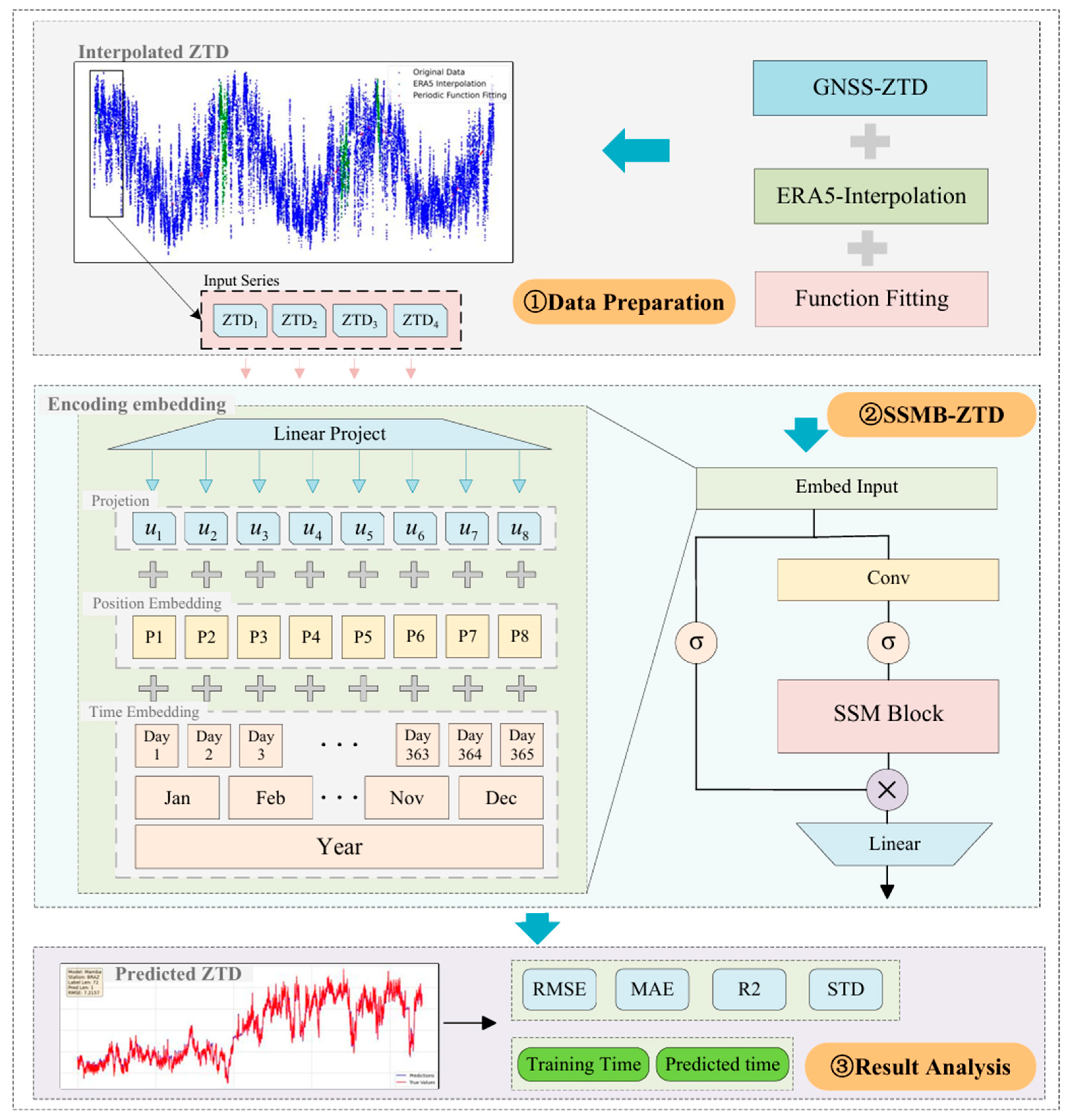
(2) A hardware-aware design is proposed, which introduces parallel scanning algorithms to realize parallel training and thus improve efficiency. A Mamba block used in this paper can be seen in Figure 4.

The proposed SSMB-ZTD model is based on the recently introduced Mamba block, a selective State Space Model (SSM) that achieves both high computational efficiency and long-range dependency modeling. However, directly using a standalone Mamba block may lead to the over-compression of historical ZTD information, weakening the model’s ability to capture subtle long-term patterns.

To address this limitation and adapt the Mamba structure to the ZTD forecasting task, we introduce a joint time–position embedding module, which effectively encodes both temporal context (e.g., seasonal and diurnal variations) and spatial information. This embedding is added to the raw ZTD input and passed through the Mamba block, enabling the model to capture complex atmospheric dynamics better. The resulting architecture, SSMB-ZTD, significantly enhances the model’s ability to model long-term dependencies in ZTD sequences while maintaining fast and scalable inference. The overall structure and flow of the model are illustrated in Figure 4.

As illustrated in Figure 4, the overall framework of SSMB-ZTD consists of three key stages: data preprocessing, temporal encoding, and model prediction. In the data preprocessing stage, raw GNSS-derived ZTD sequences undergo quality control and interpolation to fill missing values, producing a continuous time series. The cleaned time series is segmented into fixed-length input windows for use in model training and inference. Each segment is subsequently passed into the embedding module, which transforms the scalar input into a rich temporal representation.

In our implementation, each scalar ZTD value is first projected into a 512-dimensional feature vector via a 1D convolutional layer. To incorporate temporal information, we introduce two additional embeddings of the same dimension: a sinusoidal position embedding encoding-relative time steps and a learnable embedding lookup table that maps discrete time indices (e.g., hour-of-day or minute-of-day) to vector representations. The three components are integrated through element-wise addition to generate the final input embedding vector. This design enables the model to retain signal amplitude while incorporating both relative and absolute temporal structure.

This temporally enriched embedding is then fed into the selective state space model block (SSMB), which captures long-range dependencies and local patterns in the sequence. Finally, a lightweight prediction head maps the learned hidden states to future ZTD values. This modular design ensures that both physical signal continuity and temporal semantics are preserved throughout the pipeline.

3.5. Model Training

To ensure a fair and consistent comparison among models, we applied a unified data preprocessing procedure across all experiments. The dataset spans 36 months from January 2019 to December 2021, with the first 30 months used for training and validation, and the final 6 months reserved for testing. Before training, all ZTD sequences were preprocessed using the same interpolation strategy to fill missing values: short-term gaps were completed using periodic least-squares fitting, while longer gaps were reconstructed with ERA5-derived estimates, as detailed in Section 2.2.

During training, a sliding window approach (illustrated in Figure 5) was employed to generate input-output pairs: 72 h of historical ZTD values were used to predict future values at lead times of 3 h, 6 h, 12 h, 24 h, 36 h, and 48 h. No model-specific filtering, normalization, or feature engineering was applied. The raw ZTD input sequences remained identical across all models. This setup ensures that any differences in performance arise solely from the modeling architectures and learning capabilities, rather than data inconsistencies.

The models were trained on laptops equipped with NVIDIA GeForce RTX 4060 GPUs, with a fixed batch size of 16.

Table 1. Initial training parameter settings for the experimental model in this paper.

Parameter	Setting	Parameter	Setting
Mamba Block
SSM state expansion factor	16	Number of hidden dimensions	512
Convolution width	4	Dropout ratio	0.05
Train epochs	50	Label length	72
Activate function	Gelu	Loss function	MSE
Optimizer	Adam	Learning rate	0.0005
Transformer
Encoder layers	2	Decoder layers	1
Number of heads	8	Attention factor	1

presents the additional initial training parameters used. To ensure a fair comparison, the baseline training settings were kept consistent across all deep learning models.

3.6. Accuracy Evaluation Indicators

In order to evaluate the prediction performance of different models, this paper adopts the mean absolute error (MAE), root mean squared error (RMSE), standard deviation (STD), and the coefficient of determination (R²) regression evaluation indices to assess the accuracy of the prediction results. Among them, the smaller the MAE and RMSE, the smaller the model ZTD prediction value error; STD is used to measure the variability of prediction error, R² reflects the model’s fit to the fundamental changes in the data, and the closer it is to 1, the better the model fitting effect; the specific indicators are calculated as in Equations (16)–(19):

$$MAE={\displaystyle \frac{1}{n}}{\displaystyle \sum _{i=1}^n\left|ZT{D}_i-ZT{D}_i{D_i}^{pred}\right|}$$

(16)

$$RMSE=\sqrt{{\displaystyle \frac{1}{n}}{\displaystyle \sum _{i=1}^n{\left(ZT{D}_i-ZT{D_i}^{pred}\right)}^2}}$$

(17)

$$STD=\sqrt{{\displaystyle \frac{1}{N}}{\displaystyle \sum _{i=1}^N{\left(ZT{D}_i-\overline{ZT{D}_i}\right)}^2}}$$

(18)

$$R^2=1-{\displaystyle \frac{{\displaystyle \sum _{i=1}^n{\left(ZT{D}_i-ZT{D_i}^{pred}\right)}^2}}{{\displaystyle \sum _{i=1}^n{\left(ZT{D}_i-\overline{ZT{D}_i}\right)}^2}}}$$

(19)

where $ZT{D}_i$ is the i-th sample value of ZTD, $ZT{D_i}^{pred}$ is the i-th predicted value of the model output, $ZT{D}_i$ is the mean value of the sample ZTD, and $N$ is the total number of ZTD data.

4. Result

In this chapter, the ZTD prediction performance of the SSMB-ZTD model under different prediction time lengths is comprehensively evaluated and accuracy verified from multiple perspectives through multiple sets of experiments. First, compared with existing models such as Informer, Transformer, LSTM, RNN, and GPT3, SSMB-ZTD achieves the lowest RMSE and MAE under each prediction time length task, showing superior prediction accuracy. Second, in the stability analysis, SSMB-ZTD consistently maintains the lowest error in 24h within a day, indicating stronger robustness and stability to diurnal variations and time scales. Thirdly, from the regional generalizability analysis, the model performs well at most stations worldwide, especially in the continental interior and high-altitude areas, highlighting its adaptability to different geographic environments. Finally, the time–cost analysis shows that SSMB-ZTD significantly outperforms other models in both the training and prediction phases, which verifies its efficiency and practical value in long sequence processing.

To comprehensively evaluate the prediction performance of different models, we compiled the results of 3 h, 6 h, 12 h, 24 h, 36 h, and 48 h ZTD forecasts across all 27 stations. The statistical results of the average MAE are shown in

Table 2. Average MAE statistics of different models in experiments with varying lengths of prediction.

Predicted Length (h)	Average MAE (mm)
	SSMB-ZTD	Mamba	Informer	Transformer	LSTM	RNN	GPT3
3	7.57	8.01	10.01	7.89	18.58	19.97	34.23
6	10.43	11.00	11.89	10.79	20.65	21.03	34.45
12	12.27	14.75	15.15	14.93	22.78	24.65	34.36
24	19.21	19.61	19.30	19.63	26.41	28.86	34.27
36	22.03	22.36	22.08	22.81	28.05	31.20	34.53
48	23.63	24.36	23.96	24.80	28.23	33.58	34.40

. To further provide a normalized assessment of model prediction error, we compute the relative RMSE, defined as the ratio between RMSE and the dynamic range of the ZTD data. The dynamic range was determined to be 875.3 mm across the combined dataset. The corresponding relative RMSE values for all models and prediction lengths are presented in

Table 3. Relative RMSE (%) of different models with varying lengths of prediction based on harmonized dynamic range = 875.3 mm.

Predicted Length (h)	Relative RMSE (%)
	SSMB-ZTD	Mamba	Informer	Transformer	LSTM	RNN	GPT3
3	1.79	1.82	2.09	1.83	3.14	3.42	5.04
6	2.41	2.48	2.53	2.45	4.02	4.25	5.21
12	3.23	3.31	3.26	3.31	4.80	4.72	5.17
24	3.67	3.76	3.90	3.73	5.29	5.32	5.21
36	4.45	4.50	4.27	4.70	5.22	5.39	5.13
48	4.41	4.56	4.40	4.59	5.21	5.49	5.21

. As shown, the SSMB-ZTD model consistently achieves the lowest MAE and relative RMSE at all prediction horizons, demonstrating superior performance both in terms of absolute error and proportional error. Among all prediction lengths, the best performance is observed at the 12-h forecast, where the MAE of the SSMB-ZTD model is reduced by 16.80%, 19.01%, 17.80%, 46.15%, 50.24%, and 64.30% compared to the Mamba block, Informer, Transformer, LSTM, RNN, and GPT3 models, respectively. This result highlights the effectiveness of our temporal and positional embedding strategy, which enables the model to better capture both local and long-term temporal dependencies in ZTD sequences, thereby improving prediction accuracy across various forecast durations.

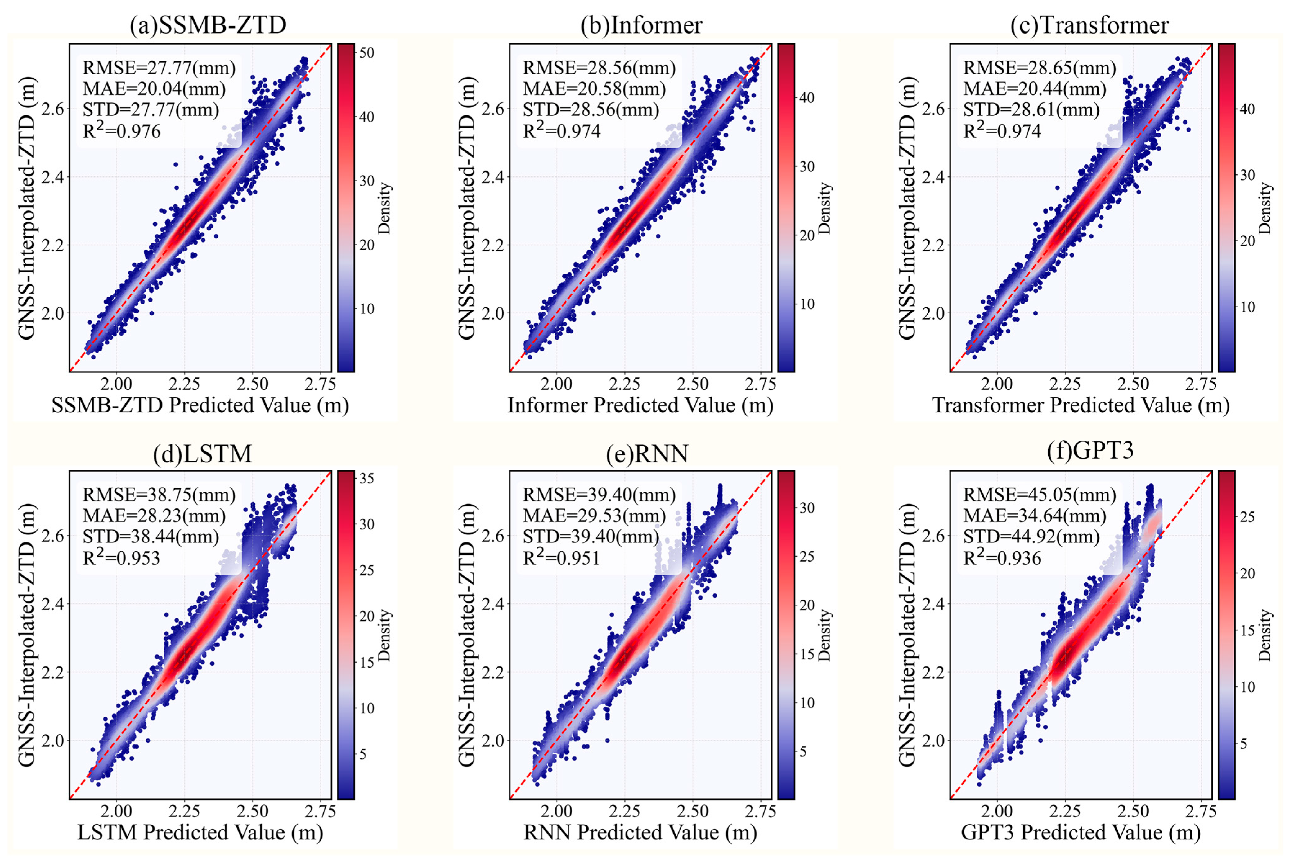
In the task with a prediction length of 12h, we selected the predicted values of each model at all stations at the moments of 0:00, 6:00, 12:00, and 18:00 to plot the point density maps to provide a visual framework for the detailed analysis of the model performance, as shown in Figure 6. By comparison, the SSMB-ZTD model proposed in this paper maintains the highest accuracy under several evaluation metrics. The overall RMSE, MAE, STD, and R2 of all stations are 27.77 mm, 20.04 mm, 27.77 mm, and 0.976, respectively. It can be seen that the points are highly clustered around the diagonal line, which indicates that the deviation between the predicted values and the true values is slight. The correlation is high, and the degree of correlation is higher, which reflects that the SSMB-ZTD proposed in this paper can accurately extract the underlying patterns in the ZTD time-series prediction task, thus obtaining the prediction results closer to the true values.

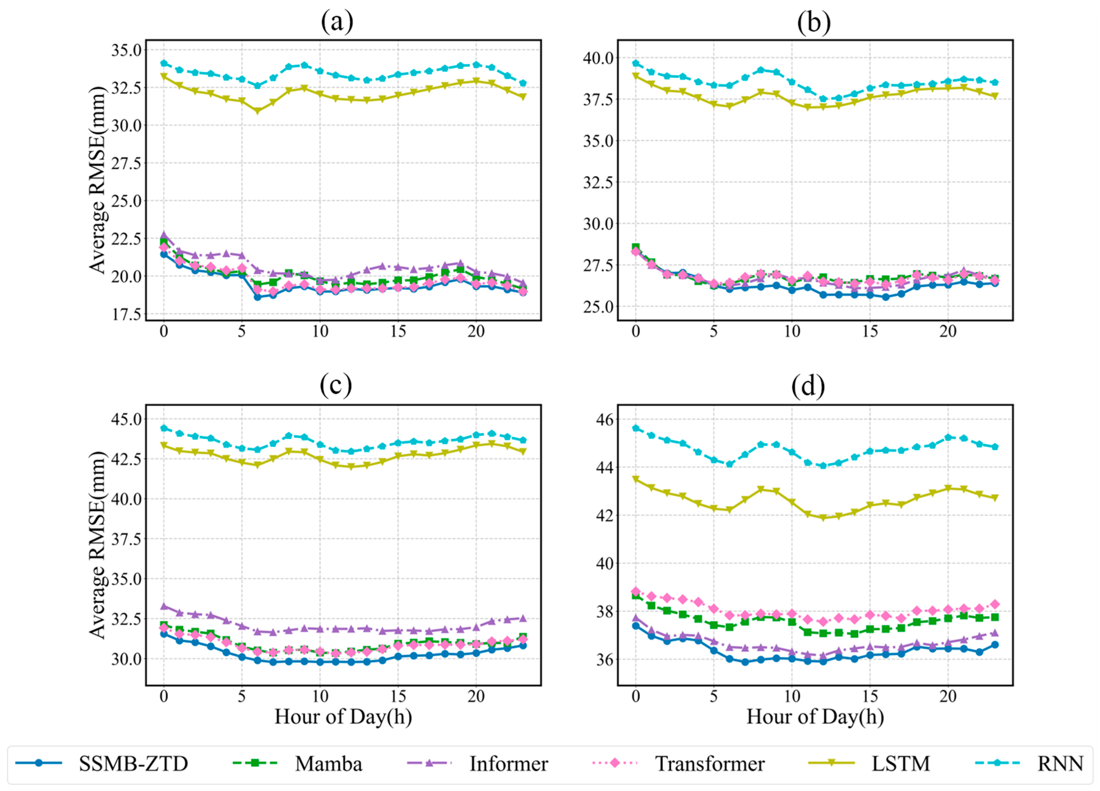
In addition, we plot the variation in the prediction RMSE of each deep learning model in different prediction lengths (6 h, 12 h, 24 h, and 48 h were selected) over 24 h in a day, as shown in Figure 7. The results show that the errors of all models increase as the prediction length increases, with the Informer, Transformer, and Mamba models having relatively low errors and the LSTM and RNN models having relatively high errors, while the SSMB-ZTD model exhibits the lowest error at all prediction lengths, which suggests that the SSMB-ZTD model proposed in this paper performs very consistently at different moments in the long ZTD sequence prediction task.

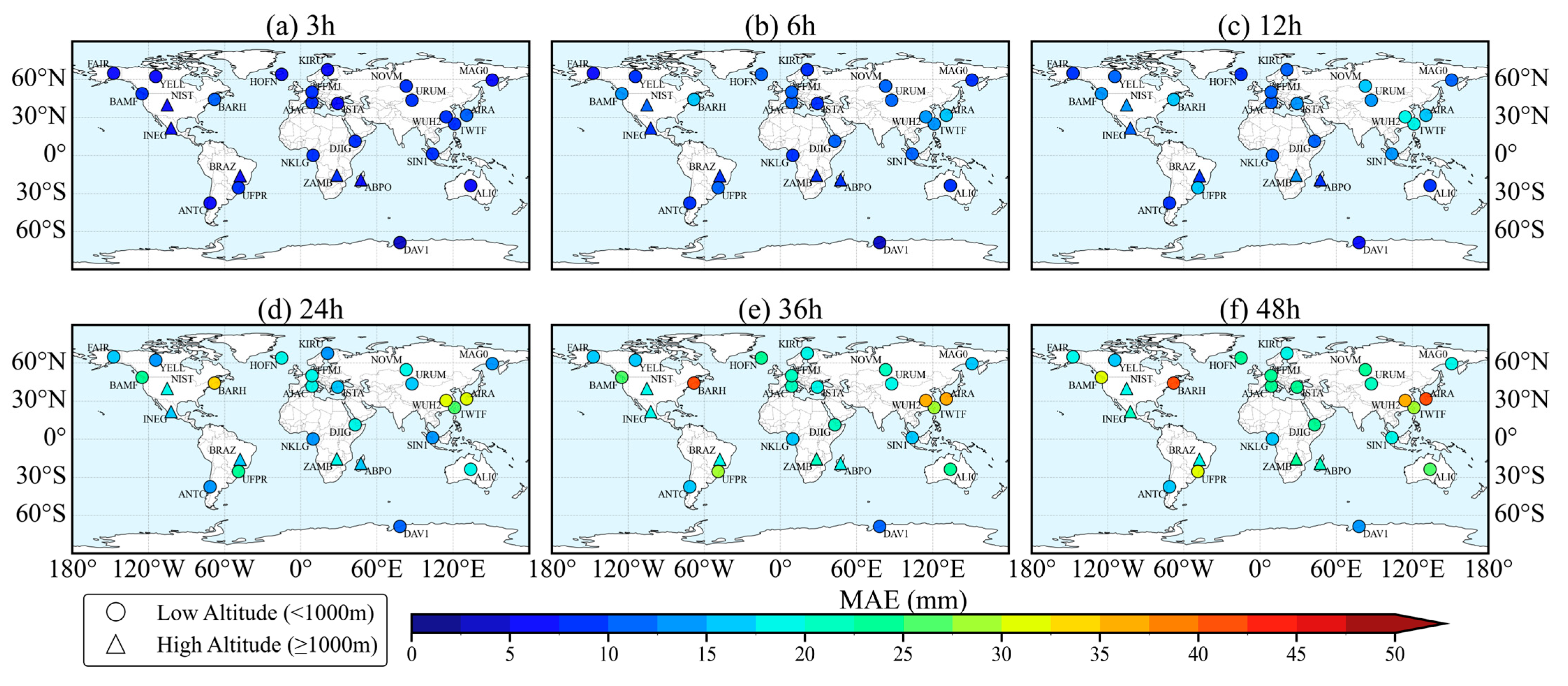
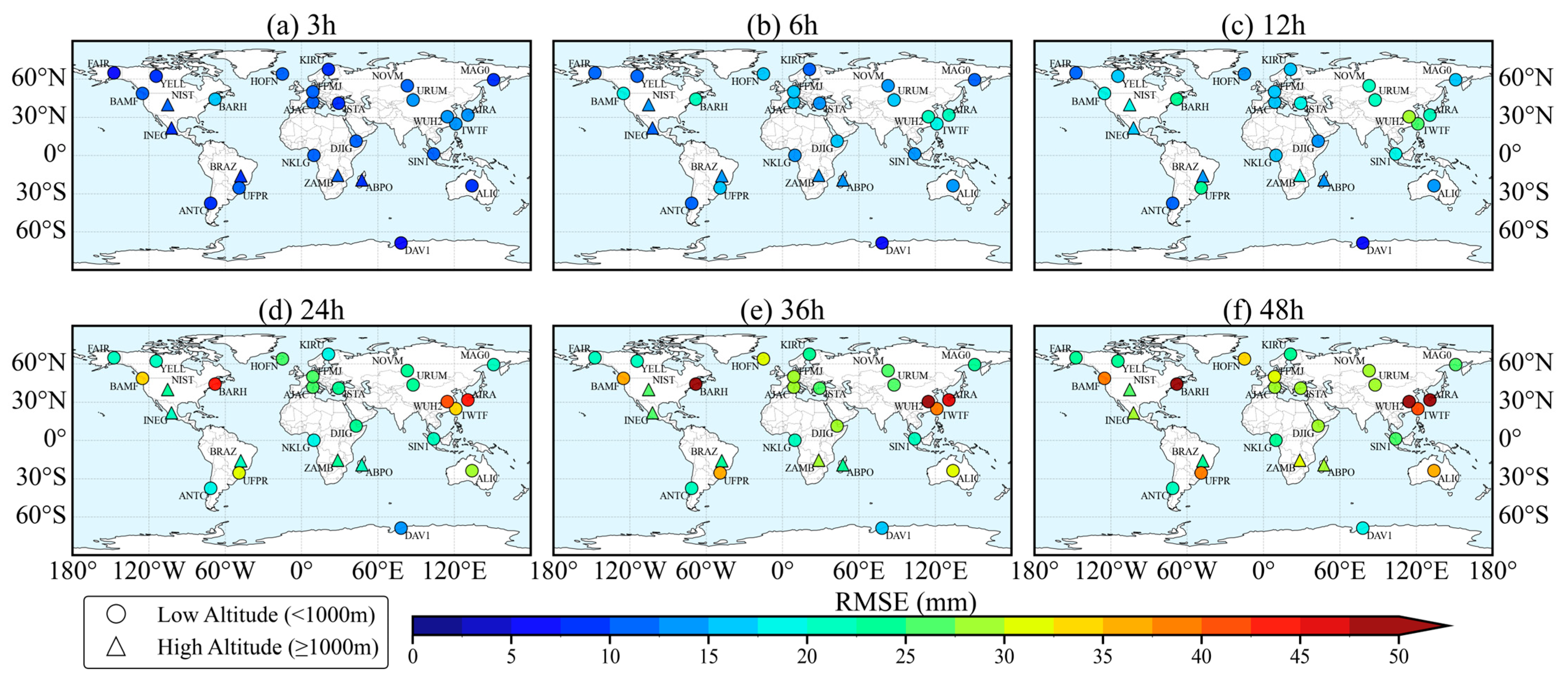
To analyze the SSMB-ZTD model’s performance across different global regions, we plotted the accuracy distribution for each station under various forecast durations, including changes in MAE and RMSE distributions. As shown in Figure 8 and Figure 9, the station color transitions from blue (lower error) to red (higher error), indicating that the RMSE and MAE as a whole tend to increase with the increase in forecast duration and the prediction accuracy of the SSMB-ZTD model gradually decreases. However, the accuracy of each station is still better than that of the empirical GPT3 model up to 48 h.

At the same time, there are noticeable spatial differences in the accuracy among the stations. As can be seen from Figure 8 and Figure 9, the overall prediction accuracies of the intra-continental sites are better than those of the coastal regions. This phenomenon can be easily understood by the fact that the coastal areas are more frequently disturbed by humid air currents [23]. In addition, the prediction accuracies of high-altitude areas (marked by triangles in the figures) are generally more stable, which may be due to the tropospheric delay being related to the altitude [43,44] and the lower water vapor content in the high-altitude areas leading to a more negligible effect of the wet delay. Its time series is more stable and the model is more likely to capture its change pattern, so the prediction accuracy is also higher.

Finally, we plotted the time cost of each model at each stage as bar charts, as in Figure 10, to visualize the efficiency of the compared models. By comparing the training and testing times of the five models—SSMB-ZTD, Informer, Transformer, LSTM, and RNN—at different prediction lengths, we found that the SSMB-ZTD model exhibits the shortest training and prediction times for all prediction lengths, showing the higher efficiency and performance of SSMB-ZTD.

Notably, while the Informer and Transformer models may have higher prediction accuracy in some cases, their longer time consumption, especially in the training phase, may limit their application in real-time demanding scenarios. In contrast, SSMB-ZTD achieves a good balance between accuracy and efficiency. In particular, SSMB-ZTD also saves 35.11%, 21.59%, 33.84%, 20.95%, and 5.56% of the training time and 34.73%, 27.32%, 40.79%, 27.95%, and 18.37% of the prediction time in different prediction tasks, respectively, with better accuracy compared to the Informer model.

The efficiency of the SSMB-ZTD model comes from its structurally optimized Mamba block, which has linear-time complexity and is well-suited for parallel execution on GPUs. Unlike attention-based models that scale quadratically with sequence length, SSMB maintains fast training and inference without compromising accuracy. As shown in Section 4 and Table 2 and Table 3, it outperforms Transformer, Informer, LSTM, RNN, and GPT3 across most forecasting lengths in both MAE and RMSE. Although differences in training time may not significantly impact all application scenarios, they may still provide an intuitive reference for future researchers. Moreover, the efficiency of SSM structures in handling long sequences supports the rationality of our model choice, which could be beneficial in large-scale or fast-updating applications.

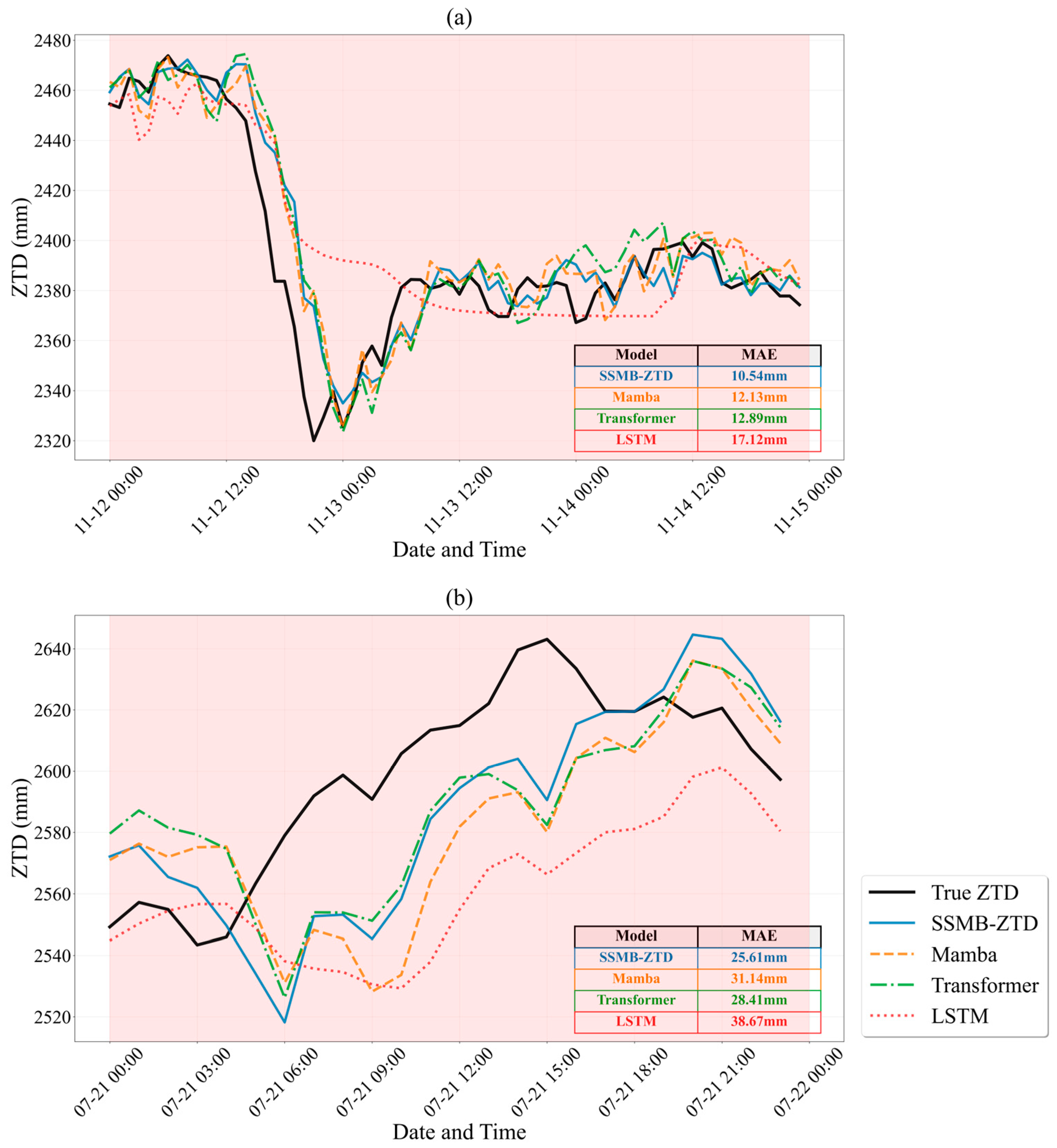
To further assess the robustness of the proposed model under extreme meteorological conditions, we conducted two case studies on heavy rainfall events. The first event occurred in Vancouver, Canada, from 12–14 November 2021. As shown in Figure 11, the shaded region highlights the rainfall period during which the ZTD exhibited sharp variations due to significant atmospheric moisture content. We compared the predictions of the SSMB-ZTD, Mamba, Transformer, and LSTM models with a prediction horizon of 3 h during this event. The results clearly demonstrate that SSMB-ZTD achieved the closest alignment with the observed ZTD curve throughout the entire rainfall period. In particular, the mean absolute error (MAE) of SSMB-ZTD was 10.54 mm, outperforming Mamba (12.13 mm), Transformer (12.89 mm), and LSTM (17.12 mm).

The second case study focused on the extreme rainfall event in Wuhan, China, in July 2021. As shown in Figure 11, the SSMB-ZTD model closely follows the observed ZTD variations throughout the entire heavy precipitation period. Specifically, the MAE of SSMB-ZTD was 25.61 mm, which is lower than that of Mamba (31.14 mm), Transformer (28.41 mm), and LSTM (38.67 mm).

The results from both the Vancouver and Wuhan scenarios demonstrate that SSMB-ZTD achieves excellent prediction performance, effectively reflecting its robustness against abrupt atmospheric changes. This case study provides additional evidence that the proposed model is not only efficient but also resilient to sudden atmospheric changes, making it a promising choice for GNSS meteorological applications.

5. Discussion

The experimental results demonstrate that the SSMB-ZTD model achieves high prediction accuracy in ZTD time-series forecasting. Consistent and stable performance is observed across various experimental settings, including different prediction lengths, geographic regions, and time periods. Furthermore, the model exhibits a significant advantage in computational efficiency. These results indicate that the integration of time stamp and position embedding effectively enhances the model’s memory of ZTD data and its ability to capture long-term dependencies, thereby validating the rationality and effectiveness of the model design. Accurate ZTD prediction is critical for GNSS positioning and GNSS meteorology. The SSMB-ZTD model proposed in this study provides more reliable atmospheric delay correction information for precise point positioning (PPP), significantly improving the accuracy of positioning results. Additionally, variations in ZTD reflect local water vapor fluctuations and climate dynamics, offering technical support for related research fields. It is worth noting that as the prediction length increases, the accuracy of ZTD prediction tends to decrease gradually. Therefore, future work should focus on validating the model’s performance under longer input windows and extended prediction horizons further to confirm the robustness and generalization capability of SSMB-ZTD.

6. Conclusions

This model integrates the efficient sequence modeling capability of the Mamba architecture with temporal and positional embedding mechanisms, enhancing the representation of long-term temporal dependencies while maintaining low computational complexity.

In this study, we conducted experiments using interpolated ZTD data from 2019 to 2022 collected at 27 global IGS stations. The results demonstrate that the SSMB-ZTD model significantly outperforms representative models such as Transformer, Informer, LSTM, and RNN across a wide range of prediction horizons (3 h to 48 h). It achieves the best performance in key evaluation metrics, particularly RMSE and MAE. Specifically, the accuracy of SSMB-ZTD is significantly higher than that of the RNN, LSTM, and GPT-3 models, with average accuracy improvements of 31.2%, 37.6%, and 48.9%, respectively. While maintaining high prediction accuracy, SSMB-ZTD also shows a clear advantage in computational efficiency during both the training and inference phases. Compared with attention-based models such as Transformer and Informer, SSMB-ZTD reduces training time by 47.6% and 21.2%, and prediction time by 38.6% and 30.0%, respectively. These results highlight the model’s strong real-time performance and potential for engineering deployment. The experiments in this paper also verify the performance of the SSMB-ZTD model across different time periods, regions, and under extreme weather conditions, such as the heavy rainfall events in Vancouver and Wuhan; the results demonstrate that the model exhibits strong stability and robustness.

In summary, the SSMB-ZTD model proposed in this paper combines high accuracy, strong generalization, and high efficiency. It provides an innovative and feasible solution for ZTD long-time-series prediction. It can be further extended to be applied in the fields of GNSS meteorological services, tropospheric modeling, and precision positioning in the future.