Abstract
The L-band radiative transfer-forward modeling plays a crucial role in data assimilation for meteorological forecasting. By utilizing information from the underlying surface (typically land surface parameters and variables), such as soil moisture, soil temperature, snow cover, freeze–thaw status, and vegetation, the corresponding brightness temperatures can be simulated through the physical processes described by radiative transfer models. Data assimilation becomes meaningful when the errors introduced by the simulated brightness temperatures are smaller than the simulation accuracy of the land surface variables. However, radiative transfer models at the L-band cannot accurately simulate TB operationally. In this study, four machine learning methods, including random forest (RF), long short-term memory (LSTM), support vector machine (SVM), and deep neural networks (DNN), are employed to reconstruct the forward relationship from land surface parameters to brightness temperatures, serving as an alternative to traditional radiative transfer models. The performance of these methods is evaluated using ground-truthed soil moisture data, soil texture static data, and leaf area index (LAI). The results indicate that DNN and RF exhibit superior performance, with DNN achieving the lowest average unbiased root mean square error (ubRMSE) of 6.238 K for vertical polarization brightness temperature (TBv) and 9.033 K for horizontal polarization brightness temperature (TBh). Regarding correlation coefficients between the retrieved brightness temperatures and satellite measurements, RF leads for H-polarized TB with a value of 0.943, while both RF and SVM perform well for V-polarized TB with values of 0.930 and 0.932, respectively. In conclusion, our study shows that DNN is the optimal method for retrieving brightness temperatures, outperforming other machine learning approaches regarding error metrics and correlation with satellite measurements. These findings highlight the potential of DNN in improving data assimilation processes in meteorological forecasting.
1. Introduction
Regarding weather and climate, the significance of land surface conditions, particularly soil moisture, cannot be overstated. Soil moisture is a crucial variable within the Earth’s system, profoundly influencing the water and energy budgets, regulating our planet’s environmental dynamics [1]. It acts as a key mediator at the land–atmosphere interface, pivotal in determining how water and energy are exchanged between the surface and the atmosphere [2]. Passive microwave observations at the L-band (1.4 GHz) have proven to be exceptionally sensitive to surface soil moisture [3], making them indispensable tools for dedicated soil moisture missions such as Soil Moisture and Ocean Salinity [4] (SMOS) and Soil Moisture Active Passive [5] (SMAP). These missions underscore the importance of accurate soil moisture measurements in understanding and predicting weather patterns and climate trends, highlighting the intricate link between the state of the land surface and the broader atmospheric conditions that shape our world.
Brightness temperature (TB) modeling has long been a central challenge in microwave remote sensing, particularly for soil moisture retrieval, freeze–thaw detection, and land–atmosphere coupling studies. Various radiative transfer (RT) models have been developed to simulate TB, with the classical τ–ω model serving as the theoretical foundation [6]. This model assumes a single scattering albedo and vegetation transmissivity, and provides a first-order approximation of the microwave emission from land surfaces.
To better account for vegetation–soil interactions and surface heterogeneity, extended models such as the τ–ω–r model [7] and the L-band Microwave Emission of the Biosphere (L-MEB) model have been proposed [8]. L-MEB, designed explicitly for the SMOS mission, introduces additional parameters to handle vegetation structure, surface roughness, and multi-angular observations [9]. Meanwhile, the Community Microwave Emission Model (CMEM) offers a modular, customizable framework widely adopted in land data assimilation systems and numerical weather prediction (NWP).
In operational systems, researchers have begun investigating the assimilation of L-band passive microwave observations from satellite missions such as SMOS and SMAP [10,11], leveraging brightness temperature (TB) data within the European Centre for Medium-Range Weather Forecasts (ECMWF) system [12,13]. To use satellite-observed TBs effectively, a forward operator must simulate TB as seen from space. CMEM has been integrated into the ECMWF system to serve this role, enabling simulation of TB at low frequencies such as 1.4 GHz. Prior studies have focused on developing and refining radiative transfer models like CMEM to construct forward operators for satellite data assimilation [14,15,16].
However, operational simulation of brightness temperature (TB) using radiative transfer models (RTMs) at the L-band is challenging due to several factors, such as (i) the complexity of the soil–vegetation–atmosphere interactions; (ii) the sensitivity of TB to surface roughness, soil moisture, and vegetation structure [17]; and (iii) the difficulty of obtaining accurate parameterizations across diverse land surface conditions [18]. These issues limit the accuracy and transferability of RTMs in operational settings [19]. Particularly in complex environments such as the Tibetan Plateau area, accurately depicting the combined influences of plant characteristics, soil moisture, and soil composition on the simulated TBs significantly constrains the model’s simulation accuracy [20].
Machine learning methods provide a way to construct observation operators by learning the relationship between system states and observed measurements from large datasets [21]. Since 2010, machine learning algorithms have gained increasing attention as data-driven approaches that can complement and enhance traditional radiative transfer models. This is primarily because machine learning methods can capture complex, nonlinear patterns within observational datasets, as demonstrated in multiple studies across soil moisture retrieval, vegetation parameter estimation, and brightness temperature simulation [22,23,24,25]. This approach can improve accuracy, reduce computational cost, and handle complex relationships more effectively [26].
This study uses machine learning models as a complementary approach to conventional radiative transfer methods for simulating brightness temperature, particularly in capturing complex nonlinear patterns from observational data. Data-driven approaches may offer improved flexibility and accuracy compared to existing physical models, which often perform poorly in complex terrains such as the Qinghai–Tibet Plateau. While still relatively underexplored, such methods are promising for advancing soil moisture remote sensing over challenging environments.
The primary objectives of this study are as follows: (1) to optimize the selection of input features and evaluate the impact of various feature combinations on the accuracy of simulated TBs; and (2) to analyze and compare the errors between TB values simulated by the deep learning model and the corresponding observed TBs. Section 2 provides a detailed overview of the Tianjun dense soil moisture sensor network in the Qinghai Lake Basin (QLB-NET) and the supporting dataset utilized in this study. Section 3 introduces the four machine learning models adopted in this study and the data partitioning strategy and evaluation metrics. Section 4 assesses the accuracy of brightness temperatures simulated by each model and compares their performance under different soil conditions. Section 5 discusses the main findings and concludes the study.
2. Materials
2.1. Study Area
To support the Qinghai Lake Basin (QLB) Water Cycle Study, the QLB-network (QLB-NET) was deployed in Tianjun, about 70 km northwest of the cited Qinghai Lake [27]. Figure 1 shows the location of the QLB-NET on the Qinghai–Tibetan Plateau, with digital elevation model (DEM) data in the background, which is derived from the Shuttle Radar Topography Mission (SRTM) data from the U.S. Space Shuttle Endeavour [28]. The area of the QLB-NET is about 36 km × 40 km, covering the SMAP antenna −3 dB beamwidth range. In addition, the distance between the QLB-NET and Qinghai Lake is 70 km, ensuring that the QLB-NET is not within the −10 dB beam range of SMAP and other microwave sensors. Thus, Qinghai Lake, which is located to the southeast of QLB-NET, will not affect the results of satellite microwave observations within the range of QLB-NET.
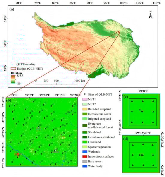
Figure 1.
(a) Geographic location of QLB-NET on the Qinghai–Tibetan Plateau (QTP), (b) distribution of sensors in the large-scale grid and two small-scale grids (NET1 and NET2) with land-cover type from GLC_FCS30-2015 in the background, (c) distribution of sensors in the small-scale grid NET1, (d) distribution of sensors in the small-scale grid NET2.
The QLB-NET is situated in the temperate semi-arid zone of the Qinghai–Tibet Plateau (QTP), where approximately one-quarter of the annual precipitation occurs during the growing season, from May to September. As illustrated in Figure 1b, the land surface within the QLB-NET is predominantly covered by grasslands, with limited agricultural land. Other land-cover types include bare soil, water bodies, urban areas, and wetlands [29]. The northern region of the QLB-NET encompasses a typical zone of excessive and unstable permafrost characterized by freeze–thaw-affected terrain and significant seasonal disturbances. Based on previous field measurements, the soil texture in the study area primarily comprises silt and fine sand, with average contents of 22% and 70%, respectively, while the clay fraction remains consistently low, at approximately 8%.
Most sensor installations within QLB-NET were completed primarily during the autumn of 2019. As illustrated in Figure 1b–d, the network comprises one large-scale grid (Figure 1b) and two small-scale grids (Figure 1c,d), covering spatial extents of approximately 36 km × 40 km and 1 km × 1 km, respectively. A total of 60 sensors were deployed within the large-scale grid and became operational in September 2019, while 22 sensors in the two small-scale grids were activated in September 2020, bringing the total number of sensor sites in QLB-NET to 82 [30].
To better understand the spatiotemporal dynamics captured by the sensor network across the study area, we analyzed the long-term variations in soil moisture and soil temperature at two depths from September 2019 to June 2023 (Figure 2). Overall, the difference in soil moisture between the two depths during the freezing season (November to March) was minimal, with both depths exhibiting average values around 0.06 m3/m3. In contrast, during the non-freezing season, soil moisture at 5 cm depth showed pronounced fluctuations, whereas values at 10 cm depth remained relatively stable. During this period, soil moisture ranged from 0.1 to 0.4 m3/m3, with standard deviations reaching up to 0.1 m3/m3, indicating considerable variability. Conversely, in the freezing season, soil moisture ranged between 0.05 and 0.1 m3/m3, with a lower standard deviation of approximately 0.02 m3/m3. This long-term dataset highlights substantial temporal variability in soil moisture, while the relatively high standard deviation underscores notable spatial variability among sensors. Similarly, soil temperature exhibited greater variability at 5 cm depth, with standard deviations during the non-freezing season averaging around 2 °C, which were higher than those observed in the freezing season. Notably, in contrast to soil moisture, the relatively small variation in soil temperature between sensors suggests limited spatial heterogeneity across the study area.
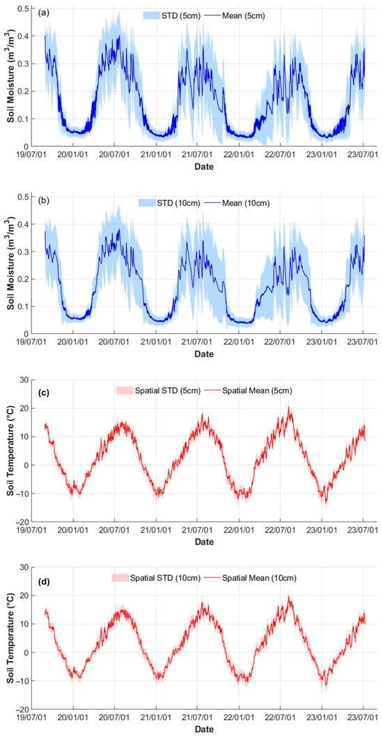
Figure 2.
A time-series plot of soil moisture/temperature and other variables relates to the TB simulation cluster of PDF (only the top two layers). (a) The time series changes of soil moisture at a depth of 5 cm in the study area from September 2019 to June 2023, (b) the time series changes of soil moisture at a depth of 10 cm in the study area from September 2019 to June 2023, (c) the time series changes of soil temperature at a depth of 5cm in the study area from September 2019 to June 2023, (d) the time series changes of soil temperature at a depth of 10cm in the study area from September 2019 to June 2023.
To ensure the reliability of the long-term soil moisture and temperature analysis, it is essential to evaluate the completeness of the dataset and address missing data issues. From September 2019 to June 2023, data availability and missing data rates were assessed for all sensors across the grid (Figure 3). Notably, the two small-scale grids became operational in September 2020, resulting in a marked increase in the volume of valid data from that point onward. In September 2020, minor fluctuations in the missing data rate were observed, primarily attributed to sensor malfunctions or physical damage [27]. To ensure continuity in the dataset, all missing values were filled using nearest-neighbor interpolation based on the geographic proximity of each sensor [31,32].
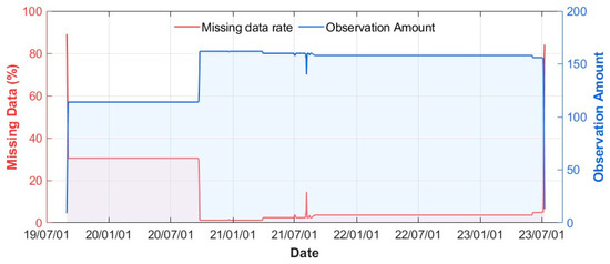
Figure 3.
Data quantity and quality exhibition from the Tianjun Network. The percentage of absence and observation period/intervals, etc.
The L-band can detect soil moisture variations within a depth range of approximately 0–20 cm [33]. Consequently, freeze–thaw dynamics occurring at any depth within this range can significantly influence the observed brightness temperature signal. From a temporal perspective, soil freeze–thaw processes can be categorized into daily and seasonal variations. In this study, we focus on seasonal freeze–thaw classification [34,35]. A “frozen” condition is one in which all monitored soil layers exhibit temperatures below −0.5 °C, and the SMAP-FT product simultaneously indicates a frozen (F) state. Taking January 1 as the reference date for frozen conditions, we applied a forward and backward temporal search from this point to identify the onset of the frozen period. All time steps following this identified onset are categorized as frozen. Conversely, a “thaw” condition is defined when all layers display temperatures above 0 °C, and the SMAP-FT product simultaneously indicates a thawed (T) state. Using August 1 as the reference thaw state, a similar bidirectional temporal search is conducted to determine the onset of the thaw period, with all subsequent time steps classified as thawed. All remaining time steps that do not satisfy the criteria for either frozen or thawed states are categorized as freeze–thaw transition periods (Table 1).

Table 1.
Illustrations of three subsets: frozen soil/thawed soil and F/T transition period.
Based on the above discriminating rules, we delineated frozen, thawed, and transition periods and plotted time-series of TB, FT state, and soil state (Figure 4). Overall, the TB values exhibit clear seasonal trends. However, in contrast to typical bare soil surfaces, the study area maintains relatively high TB values during the winter freezing period and lower TB values during the summer thawing period. The elevated TB values observed in winter are primarily attributed to the combined effects of surface snow cover and moisture-retaining frozen soils, increasing the effective emissivity. During transitional periods (spring and autumn), the temporal changes in TB values show strong consistency with the progression of freeze–thaw states, reflecting the dynamic response of microwave signals to soil phase transitions. Notably, TB values reach their annual minimum in July, which may be associated with wet and exposed surfaces and vegetation growth, which can reduce soil surface emissivity in the L-band.
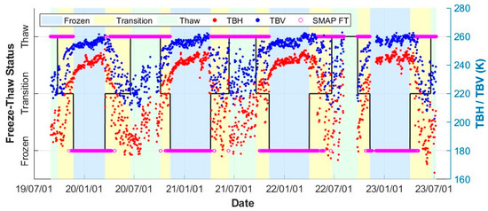
Figure 4.
Time-series plot of TB values and soil freeze–thaw state.
2.2. Auxiliary Dataset
Soil texture parameters (clay fraction, sand fraction) and surface roughness data are derived from the Soil Moisture Active Passive (SMAP) L1–L3 Ancillary Static Data, Version 1 product [36]. This product, released by the NASA Jet Propulsion Laboratory, has a spatial resolution of 36 km, is based on the Harmonized World Soil Database (HWSD) and surface features, and is widely used in passive microwave inversion to aid modeling. The leaf area index (LAI) data are derived from ERA5-Land hourly data from 1950 to the present [37], provided by the European Centre for Medium-Range Weather Forecasts (ECMWF). The dataset has a spatial resolution of 0.1° × 0.1° and an hour-by-hour temporal resolution. It is suitable for characterizing changes in surface vegetation, as derived by the meteorological reanalysis system (MRS) in conjunction with the surface processes model (SPM).
3. Methods
3.1. Machine/Deep Learning Approach
To evaluate the performance of machine learning methods in microwave brightness temperature (TB) retrieval under different soil freeze–thaw conditions, four widely used algorithms were selected in this study: deep neural network (DNN) [38], random forest (RF) [39], long short-term memory (LSTM) [40], and support vector machine (SVM) [41]. This study’s dependent variables are the L-band brightness temperatures at horizontal (TBH) and vertical (TBV) polarizations, derived from SMAP Level-3 products at a 36 km resolution. The independent variables include (1) soil moisture measurements from 82 in situ sensors within the Tianjun QLB-NET grid cell, (2) soil texture parameters (clay content and sand content), (3) surface roughness, and (4) leaf area index (LAI). All variables were spatially aggregated to match the SMAP grid and temporally synchronized with SMAP observation times. The dataset covers 30 August 2019 to 9 July 2023, with two daily time points: 6:00 a.m. and 6:00 p.m., corresponding to SMAP morning and evening overpasses. All input features were normalized prior to training to ensure numerical stability and improve model convergence.
During the model training and testing process, the dataset was first separated based on the soil freeze–thaw condition (frozen or thawed). Each soil condition’s training and testing datasets were split with different ratios for each machine learning method (Table 2). Specifically, under freeze–thaw stratification, the number of available samples in the frozen and transition categories is significantly smaller than in the thawed condition. Applying a fixed 80/10/10 split uniformly across all conditions would result in minimal testing or validation sets in low-sample subsets, increasing the risk of biased evaluation and model underfitting [42,43].
Table 2.
Proportionate division of training, testing, and validation sets under different soil freeze–thaw conditions.
In addition, each machine learning model was configured with algorithm-specific settings. The DNN consisted of 10 fully connected layers with decreasing units and ReLU activations, trained using the Adam optimizer with a learning rate of 0.001, mini-batch size of 32, and early stopping based on validation loss. The LSTM model included one LSTM layer, followed by two dense layers and a regression output layer, trained over 200 epochs with similar optimizer settings. RF was implemented using 100 regression trees via the TreeBagger function, and SVM models employed a linear kernel with built-in feature standardization. All input features were z-score normalized before training. Due to the differing architectures and training strategies, hyperparameters were tuned individually rather than presented in a unified table.
We summarized the features of the four machine learning methods considered in this study, shown in Table 3. Among the selected methods, DNN and LSTM, as deep learning approaches, can capture complex nonlinear relationships between TB and surface parameters. In contrast, traditional machine learning approaches, RF and SVM, offer good stability and interpretability, especially under relatively small sample sizes. By comparing the TB retrieval results of the four methods during the freezing and thawing periods, this study explores the accuracy of different machine learning algorithms in reconstructing the forward relationship from surface parameters to brightness temperature, providing an alternative to the traditional radiative transfer model.
Table 3.
Features of the four machine learning methods used in this study.
3.2. Evaluation Metrics
To quantitatively evaluate the performance of the TB retrieval models under different soil freeze–thaw conditions, four statistical metrics were used: root mean square error (RMSE), bias, unbiased root mean square error (ubRMSE), and the correlation coefficient (R) [57,58,59].
where E[·] is the mean processing, θs is the TB value of the SMAP satellite product, and θg is the TB value obtained from the machine learning methods retrieval. σ represents the standard deviation of TB.
3.3. Research Flowchart
Figure 5 illustrates the workflow of our study, including data processing, model implementation, and performance evaluation.
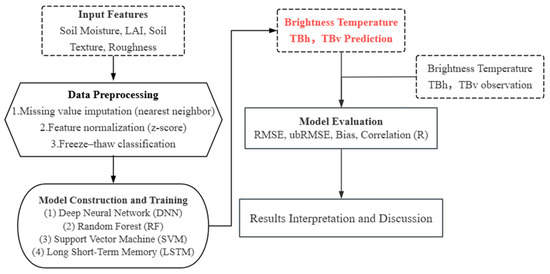
Figure 5.
Flowchart of the paper. The dashed boxes in the figure represent the data used in the research, the red font shows the prediction results of machine learning, and the arrows indicate the research process.
4. Results and Analysis
Model Performance
Based on input variables including soil moisture, static soil texture, and leaf area index (LAI), we evaluated the performance of four machine learning models—random forest (RF), long short-term memory (LSTM), support vector machine (SVM), and deep neural network (DNN)—in retrieving brightness temperature (TB). Before model training, all input variables were standardized using z-score normalization to ensure comparable feature scales. Figure 6, Figure 7 and Figure 8 present the model performance under different soil freeze–thaw conditions: frozen, thawed, and transition states, respectively. Each figure reports bias, root mean square error (RMSE), unbiased RMSE (ubRMSE), and Pearson correlation coefficient (R) for both horizontal (TBH) and vertical (TBV) polarizations. In contrast, Figure 9 summarizes the retrieval accuracy over the entire study period without distinguishing among freeze–thaw states, thus providing an integrated evaluation of the algorithm’s performance.
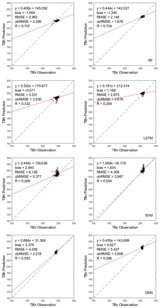
Figure 6.
Comparison of four machine learning approaches for TB simulations for frozen soil. The black dashed line represents the 1:1 reference line, indicating perfect agreement between predictions and observations. The red solid line shows the linear regression fit between predicted and observed values.
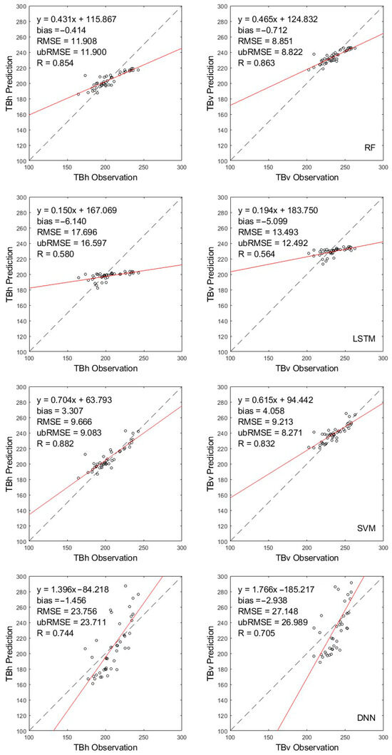
Figure 7.
Comparison of four machine learning approaches for TB simulations for thawed soil. The black dashed line represents the 1:1 reference line, indicating perfect agreement between predictions and observations. The red solid line shows the linear regression fit between predicted and observed values.
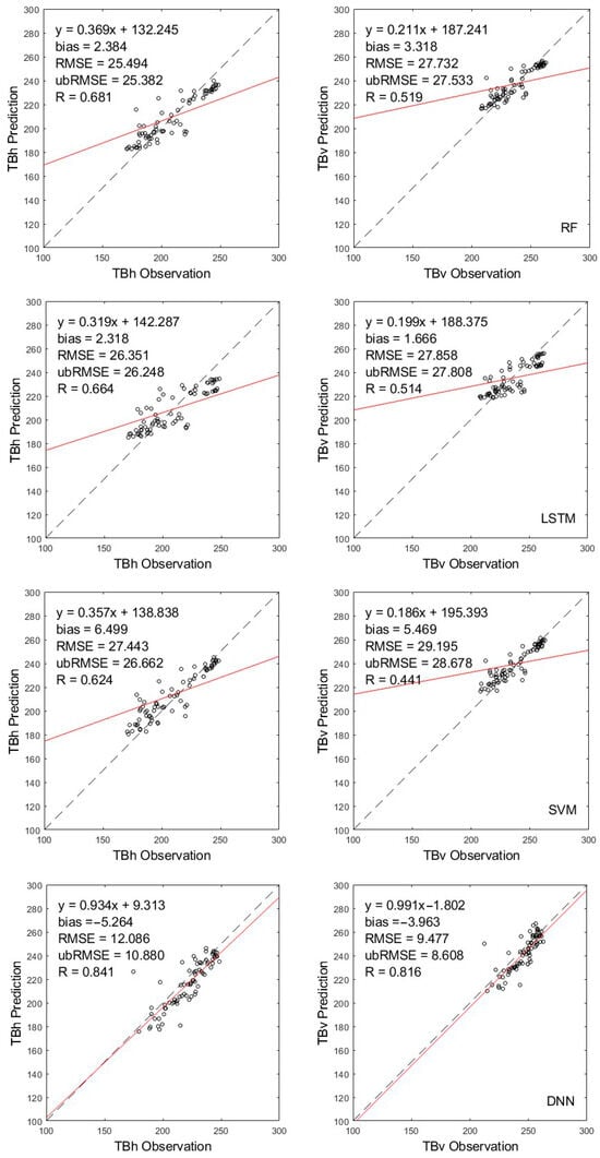
Figure 8.
Comparison of four machine learning approaches for TB simulations for the F/T transition period. The black dashed line represents the 1:1 reference line, indicating perfect agreement between predictions and observations. The red solid line shows the linear regression fit between predicted and observed values.
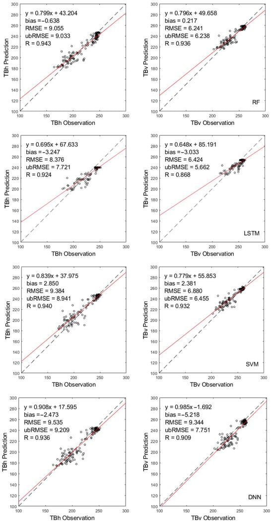
Figure 9.
Comparison of four machine learning approaches for TB retrieval. The black dashed line represents the 1:1 reference line, indicating perfect agreement between predictions and observations. The red solid line shows the linear regression fit between predicted and observed values.
Under frozen soil conditions, RF and DNN performed superiorly in simulating brightness temperatures, particularly in correlation and error stability. For TBH, RF achieved the highest correlation coefficient of 0.707 and the lowest RMSE of 2.983 K. DNN also exhibited relatively good performance, with a correlation coefficient 0.553. However, its results were affected by a noticeable positive bias of 3.376 K, suggesting a systematic overestimation. In contrast, the LSTM model had the lowest regression slope, at only 0.302. For TBV, RF again provided the best balance between accuracy and robustness, achieving the highest correlation of 0.754, a low RMSE of 2.148 K, and a slight negative bias. Although the SVM model showed a near-ideal regression slope of 1.069 for TBV, its higher RMSE of 4.309 K and a significant intercept of −16.178 K indicate a weaker overall agreement.
SVM and RF exhibited strong performance in retrieving brightness temperatures under thawed soil conditions. For TBH, SVM achieved the highest correlation coefficient of 0.882 and the lowest RMSE of 9.666 K. However, its positive bias of 3.307 K suggests a tendency toward systematic overestimation. In comparison, RF produced a slightly higher RMSE of 11.908 K but demonstrated better error stability, as indicated by a higher correlation coefficient of 0.854 and a smaller bias of −0.414 K. In contrast, DNN yielded a substantially higher RMSE of 23.756 K and a regression slope of 1.396, implying potential overfitting or limited generalization capability. For TBV, RF again provided the best balance, with a correlation coefficient of 0.863, a low RMSE of 8.851 K, and minimal bias. SVM also showed robust performance, with a high correlation of 0.832 and the lowest unbiased RMSE of 8.271 K, although a noticeable positive bias of 4.058 K was observed. On the other hand, DNN exhibited the highest RMSE of 27.148 K and an extreme slope of 1.766, while LSTM continued to show weak correlation and regression slope, indicating suboptimal retrieval under thawed conditions.
DNN performed most consistently in simulating TB under excessive soil conditions. Despite a negative bias of −5.264 K for TBH, DNN has the smallest RMSE of 12.086 K and the highest correlation coefficient of 0.841 among the four machine learning models. In contrast, RF has a larger RMSE of 25.494 K and a lower correlation coefficient of 0.681, suggesting that RF retrieval is less accurate and has a larger error dispersion type. LSTM and SVM perform even worse in this category, with RMSE values over 22K and low correlation coefficients of 0.664 and 0.624, respectively. Regarding TBV, DNN again performs the best of the four machine learning methods, with the lowest RMSE of 9.477 K and a correlation coefficient of 0.755. The regression slope of 0.991 and the intercept of −1.802 indicate that DNN’s retrieved TB values are relatively well-fitted to the satellite-observed TB values. In contrast, RF, LSTM, and SVM show significantly higher RMSEs (all higher than 21 K), weaker correlations (R < 0.52), and lower regression slopes, suggesting that the reliability of these machine learning methods is limited under transitional soil conditions.
RF and DNN demonstrated superior performance, with average ubRMSE of 9.033 K and 6.238 K for TBH and TBV, respectively, followed by values of 9.209 K and 7.751 K. LSTM and SVM exhibited relatively lower performance, with average ubRMSE values of 7.721 K and 8.941 K for TBH, and 5.662 K and 6.455 K for TBV. Regarding the ability to capture the linear relationship between the retrieved brightness temperatures and the corresponding satellite measurements, RF outperformed other models in the H-polarized brightness temperature, achieving the highest correlation coefficient of 0.943. The correlation coefficients for SVM and DNN were also high, at 0.940 and 0.936, respectively. In retrieving TBV, the correlation coefficients of both RF and SVM reach 0.930, with values of 0.936 and 0.932, respectively. DNN follows, with a correlation coefficient of 0.909. Among the three machine learning methods with correlation coefficients greater than 0.9, DNN exhibits the best performance regarding the fitted straight line for brightness temperature retrieval. The slopes of the fitted lines for TBH and TBV are remarkably close to 1, with values of 0.908 and 0.985, respectively. Additionally, the intercepts of the fitted lines are the smallest among the three methods, measuring 17.595 for TBH and −1.692 for TBV.
To reduce the randomness caused by a single train/validation split, we conducted five independent runs of each machine learning model to address this concern using randomly generated train/validation/test splits (with an 80/10/10 ratio). Figure 10 shows that the random forest (RF) model demonstrated the most stable and accurate performance across all error metrics for TBH, with the lowest RMSE and bias. LSTM and DNN exhibited greater variability, particularly in bias, while SVM showed moderate accuracy with relatively small dispersion. For TBV, RF again achieved the most consistent results, while LSTM showed noticeable instability. DNN and SVM both maintained reasonable performance but with larger fluctuations in ubRMSE and R. These results confirm the overall robustness of RF under varying data partitions for both polarizations.
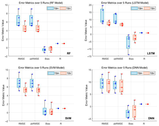
Figure 10.
Comparison of errors for each machine learning model run five times independently. The dots in the figure represent the error index values of each experiment.
In conclusion, while random forest (RF) consistently achieved the lowest RMSE, ubRMSE, and bias, and demonstrated the most stable performance across all freeze–thaw conditions, the deep neural network (DNN) model exhibited the most favorable regression slope and intercept, indicating a closer alignment between predicted and observed brightness temperatures in terms of linear fit. This suggests that although RF is more robust in minimizing absolute errors, DNN captures the underlying linear relationship more accurately. The strength of DNN lies in its ability to model complex nonlinear interactions and extract deep data features, which may be particularly advantageous in assimilation applications [60,61]. This observation aligns with recent studies highlighting the effectiveness of DNNs in remote sensing retrieval tasks [62,63,64]. Given these complementary strengths, DNN holds promise as a potential method for brightness temperature retrieval in similar applications, though further validation across diverse datasets and regions is needed. We were surprised by the relatively poor performance of LSTM in our experiments. After analysis, we attribute this to two main reasons: (1) the time-series length used in our input was relatively short and sparsely sampled (twice daily), which limits the advantages of LSTM in capturing long-term temporal dependencies; and (2) the LSTM model is more sensitive to small sample sizes and imbalanced data distribution (especially under freeze–thaw stratification), which may have led to unstable convergence.
To comprehensively evaluate the practical applicability of the machine learning models, we further compared the computational time required for brightness temperature retrieval under different soil conditions (Table 4). Across all soil states, the RF and SVM models demonstrated significantly faster execution times, with RF requiring no more than 2.49 s and SVM under 1.28 s in any case. In contrast, the DNN and LSTM models incurred substantially higher computational costs. Under frozen conditions, DNN and LSTM required 258.47 and 184.85 s, respectively, while for thawed conditions, the time increased to 287.34 s for DNN and 146.51 s for LSTM. While DNN demonstrated superior linear consistency between predicted and observed values, its higher computational cost may limit its practicality in real-time applications. In contrast, RF offers faster execution, greater stability, and competitive accuracy across different freeze–thaw conditions, making it more suitable for operational use.
Table 4.
Computation cost of RF, LSTM, SVM, and DNN.
5. Discussion and Conclusions
5.1. Comparison with Traditional Models
Traditional radiative transfer models, such as the Community Microwave Emission Model (CMEM), are widely used for simulating land surface brightness temperatures [65]. These models rely on physical parameterizations of soil moisture, vegetation, surface roughness, and atmospheric effects. However, their accuracy is often limited in complex environments, particularly under frozen soil conditions, due to simplified representations of freeze–thaw processes and assumptions about dielectric properties [16].
Several enhancements have been proposed for CMEM and related models to address these limitations. For example, Lv et al. [16] applied the CMEM-FT model to the Tibetan Plateau and reported substantial improvements in TB simulation accuracy under frozen conditions: the correlation coefficients for TBH and TBV increased from 0.53 and 0.45 to 0.85, while RMSEs decreased from 32 K and 25 K to 20 K and 15 K, respectively. Despite this improvement, the accuracy is still limited, particularly during the freeze–thaw transition period, where abrupt and nonlinear changes dominate the signal [16].
Other studies have reported similar levels of uncertainty in physical model simulations. Montzka et al. evaluated CMEM within a data assimilation framework and found that simulated TBs over European sites exhibited RMSEs between 10–18 K, depending on soil conditions [11]. Meanwhile, de Rosnay et al. integrated CMEM into the ECMWF operational system and reported global-scale TB simulation errors typically exceeding 14 K, especially over complex surfaces like forests and frozen soils [13].
By contrast, this study’s machine learning models, particularly RF and DNN, demonstrated significantly higher accuracy. When applied across all freeze–thaw conditions, RF achieved RMSEs of 9.055 K (TBH) and 6.241 K (TBV), with correlation coefficients of 0.943 and 0.936, respectively. DNN also showed strong performance with RMSEs of 9.535 K (TBH) and 9.344 K (TBV). These values represent a clear enhancement over the best-case scenarios reported for CMEM-FT and other physical models, suggesting that machine learning models are more effective in capturing the complex, nonlinear relationships in microwave emission processes, particularly in heterogeneous and freeze–thaw-affected environments.
Furthermore, the DNN model achieved regression slopes closer to unity and lower intercepts, indicating a stronger linear consistency between predicted and observed TB. While RF demonstrated lower bias and greater robustness across error metrics, DNN’s ability to align with the underlying physical response patterns may be particularly advantageous in future data assimilation applications. This observation aligns with recent studies highlighting the effectiveness of deep learning models in remote sensing radiative transfer emulation and retrieval tasks. Although this study does not include a direct comparison with physical models such as CMEM, our future work will focus on benchmarking the best-performing machine learning model identified here against radiative transfer models using the same dataset.
5.2. Limitations
Although this study has evaluated the performance of different machine learning models for simulating L-band brightness temperature under freeze–thaw conditions, some limitations still need to be addressed in future research.
First, this study’s input variable selection was based on prior knowledge and data availability. Although the chosen features demonstrated good performance across different models, further feature optimization may lead to additional improvements in accuracy and robustness. Future work will focus on systematic feature selection methods, such as recursive feature elimination, feature importance ranking, or representation learning, to construct more parsimonious and physically interpretable input sets.
Second, although this study has incorporated published results of physical models (e.g., CMEM and L-MEB) for comparison, a direct comparison under the same study area and input conditions is still lacking. This is crucial for rigorously evaluating the relative advantages of physical versus data-driven approaches. Therefore, we plan to implement parallel simulations using CMEM and machine learning models with identical input variables in future work, allowing direct benchmarking and quantitative assessment of their predictive skill.
Third, while the deep neural network (DNN) used in this study was configured based on structures validated in prior research, its architecture was selected through empirical testing. Experimental results show that model performance improved with increasing network depth up to 10 hidden layers but declined beyond 11 layers, indicating the onset of overfitting [66,67]. As a result, we adopted a 10-layer structure as the optimal design. Although Dropout layers were not included, we implemented early stopping to prevent overfitting. In future work, we will further explore regularization techniques such as Dropout and weight decay to enhance the model’s generalization capability.
Despite these limitations, the current study has made a valuable contribution by comparing four widely used machine learning models under different freeze–thaw conditions and demonstrating the feasibility of data-driven approaches in retrieving L-band brightness temperature.
5.3. Conclusions
This study assessed four machine learning models for simulating land surface brightness temperatures across different freeze–thaw conditions. Random forest (RF) exhibited the most stable and accurate performance across multiple error metrics, while deep neural networks (DNN) achieved better consistency regarding regression slope and intercept. Although DNN yielded higher average accuracy, its computational cost limits real-time applicability. In contrast, RF offers a good trade-off between efficiency and accuracy, making it more suitable for operational use in similar environments. Future work will focus on optimizing input feature selection and directly comparing the performance of machine learning models and the CMEM radiative transfer model within the same region.
Author Contributions
Conceptualization, S.L. and J.W.; Methodology, S.L. and J.W.; Formal analysis, Z.L.; Investigation, Z.L.; Resources, S.L.; Writing—original draft, S.L.; Writing—review & editing, S.L., Z.L. and J.W.; Visualization, Z.L.; Funding acquisition, S.L. All authors have read and agreed to the published version of the manuscript.
Funding
This research was funded by the Key Research and Development and Achievement Transformation Program of Inner Mongolia Autonomous Region, China (Grant No. 2025YFDZ0007); the Yan Liyuan–ENSKY Foundation Project of Zhuhai Fudan Innovation Research Institute (Grant No. JX240002); the National Key R&D Program of China (Grant No. 2022YFF0801404); and the National Natural Science Foundation of China (Grant No. 42075150).
Data Availability Statement
Publicly available datasets were used in this study. This data can be found here: (1) The SMAP dataset can be obtained at https://nsidc.org/data/spl3smp/versions/9 (From 1 September 2019 to 7 July 2023) and https://nsidc.org/data/spl3ftp/versions/4 (From 1 September 2019 to 7 July 2023). (2) The soil texture dataset can be obtained at https://nsidc.org/data/smap_l1_l3_anc_static/versions/1 (From 1 September 2019 to 7 July 2023). (3) ERA5-Land dataset can be obtained at https://cds.climate.copernicus.eu/datasets/reanalysis-era5-land?tab=overview (From 1 September 2019 to 7 July 2023). (4) Soil moisture dataset can be obtained at https://data.tpdc.ac.cn/zh-hans/data/733cf5c1-5279-4c28-8540-87725b40a966 (From 1 September 2019 to 7 July 2023). The datasets generated during and/or analyzed during the current study are available from the corresponding author on reasonable request.
Acknowledgments
We want to acknowledge the valuable support and contributions during the field experiments provided by Shaomin Liu, Zhongli Zhu, Ziwei Xu, and Linna Chai from Beijing Normal University, as well as Rui Jin from the Northwest Institute of Eco-Environment and Resources, Chinese Academy of Sciences.
Conflicts of Interest
Author Zixi Liu was employed by the company Suzhou Fuye Technology Co., Ltd. The remaining authors declare that the research was conducted in the absence of any commercial or financial relationships that could be construed as a potential conflict of interest.
References
- Seneviratne, S.I.; Corti, T.; Davin, E.L.; Hirschi, M.; Jaeger, E.B.; Lehner, I.; Orlowsky, B.; Teuling, A.J. Investigating soil moisture–climate interactions in a changing climate: A review. Earth Sci. Rev. 2010, 99, 125–161. [Google Scholar] [CrossRef]
- McColl, K.A.; Alemohammad, S.H.; Akbar, R.; Konings, A.G.; Yueh, S.; Entekhabi, D. The global distribution and dynamics of surface soil moisture. Nat. Geosci. 2017, 10, 100–104. [Google Scholar] [CrossRef]
- Calvet, J.C.; Wigneron, J.P.; Walker, J.; Karbou, F.; Chanzy, A.; Albergel, C. Sensitivity of Passive Microwave Observations to Soil Moisture and Vegetation Water Content: L-Band to W-Band. IEEE Trans. Geosci. Remote Sens. 2011, 49, 1190–1199. [Google Scholar] [CrossRef]
- Mecklenburg, S.; Drusch, M.; Kaleschke, L.; Rodriguez-Fernandez, N.; Reul, N.; Kerr, Y.; Font, J.; Martin-Neira, M.; Oliva, R.; Daganzo-Eusebio, E.; et al. ESA’s Soil Moisture and Ocean Salinity mission: From science to operational applications. Remote Sens. Environ. 2016, 180, 3–18. [Google Scholar] [CrossRef]
- Entekhabi, D.; Njoku, E.G.; Neill, P.E.O.; Kellogg, K.H.; Crow, W.T.; Edelstein, W.N.; Entin, J.K.; Goodman, S.D.; Jackson, T.J.; Johnson, J.; et al. The Soil Moisture Active Passive (SMAP) Mission. Proc. IEEE 2010, 98, 704–716. [Google Scholar] [CrossRef]
- Mo, T.; Choudhury, B.J.; Schmugge, T.J.; Wang, J.R.; Jackson, T.J. A model for microwave emission from vegetation-covered fields. J. Geophys. Res. Ocean. 1982, 87, 11229–11237. [Google Scholar] [CrossRef]
- Wigneron, J.-P.; Chanzy, A.; Calvet, J.-C.; Bruguier, N. A simple algorithm to retrieve soil moisture and vegetation biomass using passive microwave measurements over crop fields. Remote Sens. Environ. 1995, 51, 331–341. [Google Scholar] [CrossRef]
- Wigneron, J.P.; Kerr, Y.; Waldteufel, P.; Saleh, K.; Escorihuela, M.J.; Richaume, P.; Ferrazzoli, P.; de Rosnay, P.; Gurney, R.; Calvet, J.C.; et al. L-band Microwave Emission of the Biosphere (L-MEB) Model: Description and calibration against experimental data sets over crop fields. Remote Sens. Environ. 2007, 107, 639–655. [Google Scholar] [CrossRef]
- Wang, J.R.; Engman, E.T.; Mo, T.; Schmugge, T.J.; Shiue, J.C. The Effects of Soil Moisture, Surface Roughness, and Vegetation on L-Band Emission and Backscatter. IEEE Trans. Geosci. Remote Sens. 1987, GE-25, 825–833. [Google Scholar] [CrossRef]
- Wigneron, J.-P.; Chanzy, A.; Calvet, J.-C.; Olioso, A.; Kerr, Y. Modeling approaches to assimilating L band passive microwave observations over land surfaces. J. Geophys. Res. Atmos. 2002, 107, ACL 11-1–ACL 11-14. [Google Scholar] [CrossRef]
- Montzka, C.; Grant, J.P.; Moradkhani, H.; Franssen, H.-J.H.; Weihermüller, L.; Drusch, M.; Vereecken, H. Estimation of Radiative Transfer Parameters from L-Band Passive Microwave Brightness Temperatures Using Advanced Data Assimilation. Vadose Zone J. 2013, 12, 1–17. [Google Scholar] [CrossRef]
- Muñoz-Sabater, J.; Lawrence, H.; Albergel, C.; Rosnay, P.; Isaksen, L.; Mecklenburg, S.; Kerr, Y.; Drusch, M. Assimilation of SMOS brightness temperatures in the ECMWF Integrated Forecasting System. Q. J. R. Meteorol. Soc. 2019, 145, 2524–2548. [Google Scholar] [CrossRef]
- de Rosnay, P.; Muñoz-Sabater, J.; Albergel, C.; Isaksen, L.; English, S.; Drusch, M.; Wigneron, J.-P. SMOS brightness temperature forward modelling and long term monitoring at ECMWF. Remote Sens. Environ. 2020, 237, 111424. [Google Scholar] [CrossRef]
- Kornelsen, K.C.; Davison, B.; Coulibaly, P. Application of SMOS Soil Moisture and Brightness Temperature at High Resolution With a Bias Correction Operator. IEEE J. Sel. Top. Appl. Earth Obs. Remote Sens. 2016, 9, 1590–1605. [Google Scholar] [CrossRef]
- Albergel, C.; Balsamo, G.; de Rosnay, P.; Muñoz-Sabater, J.; Boussetta, S. A bare ground evaporation revision in the ECMWF land-surface scheme: Evaluation of its impact using ground soil moisture and satellite microwave data. Hydrol. Earth Syst. Sci. 2012, 16, 3607–3620. [Google Scholar] [CrossRef]
- Lv, S.; Simmer, C.; Zeng, Y.; Wen, J.; Su, Z. The Simulation of L-Band Microwave Emission of Frozen Soil during the Thawing Period with the Community Microwave Emission Model (CMEM). J. Remote Sens. 2022, 2022, 9754341. [Google Scholar] [CrossRef]
- Jackson, T.J.; Schmugge, T.J. Vegetation effects on the microwave emission of soils. Remote Sens. Environ. 1991, 36, 203–212. [Google Scholar] [CrossRef]
- Pampaloni, P.; Paloscia, S. Microwave Emission and Plant Water Content: A Comparison between Field Measurements and Theory. IEEE Trans. Geosci. Remote Sens. 1986, GE-24, 900–905. [Google Scholar] [CrossRef]
- Jackson, T.J.; Bindlish, R.; Cosh, M.H.; Zhao, T.; Starks, P.J.; Bosch, D.D.; Seyfried, M.; Moran, M.S.; Goodrich, D.C.; Kerr, Y.H.; et al. Validation of Soil Moisture and Ocean Salinity (SMOS) Soil Moisture Over Watershed Networks in the U.S. IEEE Trans. Geosci. Remote Sens. 2012, 50, 1530–1543. [Google Scholar] [CrossRef]
- Chen, Y.; Yang, K.; Qin, J.; Cui, Q.; Lu, H.; La, Z.; Han, M.; Tang, W. Evaluation of SMAP, SMOS, and AMSR2 soil moisture retrievals against observations from two networks on the Tibetan Plateau. J. Geophys. Res. Atmos. 2017, 122, 5780–5792. [Google Scholar] [CrossRef]
- Sarker, I.H. Machine Learning: Algorithms, Real-World Applications and Research Directions. SN Comput. Sci. 2021, 2, 160. [Google Scholar] [CrossRef]
- Xue, Y.; Forman, B.A. Comparison of passive microwave brightness temperature prediction sensitivities over snow-covered land in North America using machine learning algorithms and the Advanced Microwave Scanning Radiometer. Remote Sens. Environ. 2015, 170, 153–165. [Google Scholar] [CrossRef]
- Forman, B.A.; Reichle, R.H.; Derksen, C. Estimating Passive Microwave Brightness Temperature Over Snow-Covered Land in North America Using a Land Surface Model and an Artificial Neural Network. IEEE Trans. Geosci. Remote Sens. 2014, 52, 235–248. [Google Scholar] [CrossRef]
- Ali, I.; Greifeneder, F.; Stamenkovic, J.; Neumann, M.; Notarnicola, C. Review of Machine Learning Approaches for Biomass and Soil Moisture Retrievals from Remote Sensing Data. Remote Sens. 2015, 7, 16398–16421. [Google Scholar] [CrossRef]
- Srivastava, P.K.; Han, D.; Ramirez, M.R.; Islam, T. Machine Learning Techniques for Downscaling SMOS Satellite Soil Moisture Using MODIS Land Surface Temperature for Hydrological Application. Water Resour. Manag. 2013, 27, 3127–3144. [Google Scholar] [CrossRef]
- Janiesch, C.; Zschech, P.; Heinrich, K. Machine learning and deep learning. Electron. Mark. 2021, 31, 685–695. [Google Scholar] [CrossRef]
- Chai, L.; Zhu, Z.; Liu, S.; Xu, Z.; Jin, R.; Li, X.; Kang, J.; Che, T.; Zhang, Y.; Zhang, J.; et al. QLB-NET: A Dense Soil Moisture and Freeze–Thaw Monitoring Network in the Qinghai Lake Basin on the Qinghai–Tibetan Plateau. Bull. Am. Meteorol. Soc. 2024, 105, E584–E604. [Google Scholar] [CrossRef]
- Farr, T.G.; Kobrick, M. Shuttle radar topography mission produces a wealth of data. Eos Trans. Am. Geophys. Union 2000, 81, 583–585. [Google Scholar] [CrossRef]
- Liangyun, L.; Xiao, Z.; Xidong, C.; Yuan, G.; Jun, M. GLC_FCS30: Global Land-Cover Product with Fine Classification System at 30 m Using Time-Series Landsat Imagery; Zenodo: Geneva, Switzerland, 2020. [Google Scholar] [CrossRef]
- Liu, S.; Zhu, Z.; Xu, Z.; Jin, R.; Chai, L. Dataset of Tianjun Dense Soil Moisture and Freeze–Thaw Monitoring Network in the Qinghai Lake Basin (QLB-NET) (2019–2023); National Tibetan Plateau/Third Pole Environment Data Center: Beijing, China, 2024. [Google Scholar] [CrossRef]
- Beretta, L.; Santaniello, A. Nearest neighbor imputation algorithms: A critical evaluation. BMC Med. Inform. Decis. Mak. 2016, 16, 74. [Google Scholar] [CrossRef] [PubMed]
- Parsania, P.S.; Virparia, P.V. A comparative analysis of image interpolation algorithms. Int. J. Adv. Res. Comput. Commun. Eng. 2016, 5, 29–34. [Google Scholar] [CrossRef]
- Zheng, D.; Li, X.; Wang, X.; Wang, Z.; Wen, J.; van der Velde, R.; Schwank, M.; Su, Z. Sampling depth of L-band radiometer measurements of soil moisture and freeze-thaw dynamics on the Tibetan Plateau. Remote Sens. Environ. 2019, 226, 16–25. [Google Scholar] [CrossRef]
- Lv, S.; Zhao, T.; Hu, Y.; Wen, J. Assessing the Freeze–Thaw Dynamics With the Diurnal Amplitude Variations Algorithm Utilizing NEON Soil Temperature Profiles. IEEE J. Sel. Top. Appl. Earth Obs. Remote Sens. 2025, 18, 7904–7916. [Google Scholar] [CrossRef]
- Lv, S.; Simmer, C.; Zeng, Y.; Wen, J.; Guo, Y.; Su, Z. A Novel Global Freeze-Thaw State Detection Algorithm Based on Passive L-Band Microwave Remote Sensing. Cryosphere Discuss. 2022, 2022, 1–25. [Google Scholar] [CrossRef]
- Peng, J.; Mohammed, P.; Chaubell, J.; Chan, S.; Kim, S.; Das, N.; Dunbar, S.; Bindlish, R.; Xu, X. Soil Moisture Active Passive (SMAP) L1–L3 Ancillary Static Data, Version 1; NSIDC: Boulder, CO, USA, 2019. [Google Scholar] [CrossRef]
- Copernicus Climate Change Service. ERA5-Land Hourly Data from 1950 to Present; Copernicus Climate Change Service: Reading, UK, 2019. [Google Scholar] [CrossRef]
- Sze, V.; Chen, Y.H.; Yang, T.J.; Emer, J.S. Efficient Processing of Deep Neural Networks: A Tutorial and Survey. Proc. IEEE 2017, 105, 2295–2329. [Google Scholar] [CrossRef]
- Biau, G.; Scornet, E. A random forest guided tour. TEST 2016, 25, 197–227. [Google Scholar] [CrossRef]
- Hochreiter, S.; Schmidhuber, J. Long Short-Term Memory. Neural Comput. 1997, 9, 1735–1780. [Google Scholar] [CrossRef]
- Noble, W.S. What is a support vector machine? Nat. Biotechnol. 2006, 24, 1565–1567. [Google Scholar] [CrossRef] [PubMed]
- Reichstein, M.; Camps-Valls, G.; Stevens, B.; Jung, M.; Denzler, J.; Carvalhais, N.; Prabhat. Deep learning and process understanding for data-driven Earth system science. Nature 2019, 566, 195–204. [Google Scholar] [CrossRef]
- Pelletier, C.; Webb, G.I.; Petitjean, F. Temporal Convolutional Neural Network for the Classification of Satellite Image Time Series. Remote Sens. 2019, 11, 523. [Google Scholar] [CrossRef]
- Breiman, L. Random Forests. Mach. Learn. 2001, 45, 5–32. [Google Scholar] [CrossRef]
- Belgiu, M.; Drăguţ, L. Random forest in remote sensing: A review of applications and future directions. ISPRS J. Photogramm. Remote Sens. 2016, 114, 24–31. [Google Scholar] [CrossRef]
- Liu, Y.; Wang, Y.; Zhang, J. New Machine Learning Algorithm: Random Forest. In Proceedings of the Information Computing and Applications (ICICA 2012), Chengde, China, 14–16 September 2012; pp. 246–252. [Google Scholar]
- Van Houdt, G.; Mosquera, C.; Nápoles, G. A review on the long short-term memory model. Artif. Intell. Rev. 2020, 53, 5929–5955. [Google Scholar] [CrossRef]
- Sherstinsky, A. Fundamentals of Recurrent Neural Network (RNN) and Long Short-Term Memory (LSTM) network. Phys. D Nonlinear Phenom. 2020, 404, 132306. [Google Scholar] [CrossRef]
- Filipović, N.; Brdar, S.; Mimić, G.; Marko, O.; Crnojević, V. Regional soil moisture prediction system based on Long Short-Term Memory network. Biosyst. Eng. 2022, 213, 30–38. [Google Scholar] [CrossRef]
- Tian, Y.; Yong, S.; Liu, X. Recent advances on support vector machines research. Technol. Econ. Dev. Econ. 2012, 18, 5–33. [Google Scholar] [CrossRef]
- Gholami, R.; Fakhari, N. Chapter 27—Support Vector Machine: Principles, Parameters, and Applications. In Handbook of Neural Computation; Samui, P., Sekhar, S., Balas, V.E., Eds.; Academic Press: Cambridge, MA, USA, 2017; pp. 515–535. [Google Scholar]
- Mountrakis, G.; Im, J.; Ogole, C. Support vector machines in remote sensing: A review. ISPRS J. Photogramm. Remote Sens. 2011, 66, 247–259. [Google Scholar] [CrossRef]
- Miikkulainen, R.; Liang, J.; Meyerson, E.; Rawal, A.; Fink, D.; Francon, O.; Raju, B.; Shahrzad, H.; Navruzyan, A.; Duffy, N.; et al. 14—Evolving deep neural networks. In Artificial Intelligence in the Age of Neural Networks and Brain Computing, 2nd ed.; Kozma, R., Alippi, C., Choe, Y., Morabito, F.C., Eds.; Academic Press: Cambridge, MA, USA, 2024; pp. 269–287. [Google Scholar]
- Zhou, X.; Qin, A.K.; Gong, M.; Tan, K.C. A Survey on Evolutionary Construction of Deep Neural Networks. IEEE Trans. Evol. Comput. 2021, 25, 894–912. [Google Scholar] [CrossRef]
- LeCun, Y.; Bengio, Y.; Hinton, G. Deep learning. Nature 2015, 521, 436–444. [Google Scholar] [CrossRef] [PubMed]
- Fischetti, M.; Jo, J. Deep neural networks and mixed integer linear optimization. Constraints 2018, 23, 296–309. [Google Scholar] [CrossRef]
- Ma, H.; Zeng, J.; Zhang, X.; Peng, J.; Li, X.; Fu, P.; Cosh, M.H.; Letu, H.; Wang, S.; Chen, N.; et al. Surface soil moisture from combined active and passive microwave observations: Integrating ASCAT and SMAP observations based on machine learning approaches. Remote Sens. Environ. 2024, 308, 114197. [Google Scholar] [CrossRef]
- Lojou, J.Y.; Bernard, R.; Eymard, L. A Simple Method for Testing Brightness Temperatures from Satellite Microwave Radiometers. J. Atmos. Ocean. Technol. 1994, 11, 387–400. [Google Scholar] [CrossRef]
- Pellarin, T.; Kerr, Y.H.; Wigneron, J.P. Global Simulation of Brightness Temperatures at 6.6 and 10.7 GHz Over Land Based on SMMR Data Set Analysis. IEEE Trans. Geosci. Remote Sens. 2006, 44, 2492–2505. [Google Scholar] [CrossRef]
- Chen, C.-H.; Lai, J.-P.; Chang, Y.-M.; Lai, C.-J.; Pai, P.-F. A Study of Optimization in Deep Neural Networks for Regression. Electronics 2023, 12, 3071. [Google Scholar] [CrossRef]
- Farrell, M.H.; Liang, T.; Misra, S. Deep Neural Networks for Estimation and Inference. Econometrica 2021, 89, 181–213. [Google Scholar] [CrossRef]
- Xu, X.; Sun, X.; Han, W.; Zhong, X.; Chen, L.; Gao, Z.; Li, H. FuXi-DA: A generalized deep learning data assimilation framework for assimilating satellite observations. npj Clim. Atmos. Sci. 2025, 8, 156. [Google Scholar] [CrossRef]
- Liang, X.; Garrett, K.; Liu, Q.; Maddy, E.S.; Ide, K.; Boukabara, S. A Deep-Learning-Based Microwave Radiative Transfer Emulator for Data Assimilation and Remote Sensing. IEEE J. Sel. Top. Appl. Earth Obs. Remote Sens. 2022, 15, 8819–8833. [Google Scholar] [CrossRef]
- Stegmann, P.G.; Johnson, B.; Moradi, I.; Karpowicz, B.; McCarty, W. A deep learning approach to fast radiative transfer. J. Quant. Spectrosc. Radiat. Transf. 2022, 280, 108088. [Google Scholar] [CrossRef]
- Holmes, T.R.H.; Drusch, M.; Wigneron, J.P.; Jeu, R.A.M.d. A Global Simulation of Microwave Emission: Error Structures Based on Output from ECMWF’s Operational Integrated Forecast System. IEEE Trans. Geosci. Remote Sens. 2008, 46, 846–856. [Google Scholar] [CrossRef]
- Uzair, M.; Jamil, N. Effects of Hidden Layers on the Efficiency of Neural networks. In Proceedings of the 2020 IEEE 23rd International Multitopic Conference (INMIC), Bahawalpur, Pakistan, 5–7 November 2020; pp. 1–6. [Google Scholar]
- Schilling, A.; Metzner, C.; Rietsch, J.; Gerum, R.; Schulze, H.; Krauss, P. How deep is deep enough?—Quantifying class separability in the hidden layers of deep neural networks. arXiv 2018, arXiv:1811.01753. [Google Scholar]
Disclaimer/Publisher’s Note: The statements, opinions and data contained in all publications are solely those of the individual author(s) and contributor(s) and not of MDPI and/or the editor(s). MDPI and/or the editor(s) disclaim responsibility for any injury to people or property resulting from any ideas, methods, instructions or products referred to in the content. |
© 2025 by the authors. Licensee MDPI, Basel, Switzerland. This article is an open access article distributed under the terms and conditions of the Creative Commons Attribution (CC BY) license (https://creativecommons.org/licenses/by/4.0/).