Spatially Interpolated CYGNSS Data Improve Downscaled 3 km SMAP/CYGNSS Soil Moisture

Abstract

Soil moisture data with both a fine spatial scale and a short global repeat period would benefit many hydrologic and climatic applications. Since the radar transmitter malfunctioned on NASA’s Soil Moisture Active Passive (SMAP) in 2015, SMAP soil moisture has been downscaled using numerous alternative fine-resolution data. In this paper, we describe the creation and validation of a new downscaled 3 km soil moisture dataset, which is the culmination of previous work. We downscaled SMAP enhanced 9 km brightness temperatures by merging them with L-band Cyclone Global Navigation Satellite System (CYGNSS) reflectivity data, using a modified version of the SMAP active–passive brightness temperature algorithm. We then calculated 3 km SMAP/CYGNSS soil moisture using the resulting 3 km SMAP/CYGNSS brightness temperatures and the SMAP single-channel vertically polarized soil moisture algorithm (SCA-V). To remedy the sparse daily coverage of CYGNSS data at a 3 km spatial resolution, we used spatially interpolated CYGNSS data to downscale SMAP soil moisture. 3 km interpolated SMAP/CYGNSS soil moisture matches the SMAP repeat period of ~2–3 days, providing a soil moisture dataset with both a fine spatial scale and a short repeat period. 3 km interpolated SMAP/CYGNSS soil moisture, upscaled to 9 km, has an average correlation of 0.82 and an average unbiased root mean square difference (ubRMSD) of 0.035 cm³/cm³ using all SMAP 9 km core validation sites (CVSs) within ±38° latitude. The observed (not interpolated) SMAP/CYGNSS soil moisture did not perform as well at the SMAP 9 km CVSs, with an average correlation of 0.68 and an average ubRMSD of 0.048 cm³/cm³. A sensitivity analysis shows that CYGNSS reflectivity is likely responsible for most of the uncertainty in downscaled SMAP/CYGNSS soil moisture. The success of 3 km SMAP/CYGNSS soil moisture demonstrates that Global Navigation Satellite System–Reflectometry (GNSS-R) observations are effective for downscaling soil moisture.

1. Introduction

Global satellite soil moisture monitoring with both fine spatial resolution and short global repeat periods would benefit hydrologic and climatic monitoring, water resources management, weather and climate prediction, flood, drought, and fire monitoring and prediction, and agricultural monitoring [1]. However, most soil moisture monitoring satellites do not provide both fine spatial resolution and short repeat periods. Soil moisture retrieved from passive brightness temperatures, like those observed by the Soil Moisture and Ocean Salinity (SMOS) mission [2] and the Advanced Microwave Scanning Radiometer (AMSR-E) on the Aqua satellite [3], has short repeat periods (~2–3 days) but relatively coarse spatial resolution (~40–60 km). In contrast, soil moisture retrieved from active backscatter signals, like those observed by Sentinel-1 [4] and the planned NASA-ISRO Synthetic Aperture Radar (NISAR) mission [5], has relatively fine spatial resolution (~100 m–1 km) but long repeat periods (~6–12 days). Combining the passive and active retrieval methods is required to provide soil moisture with both fine spatial resolution and short global repeat periods.

The Soil Moisture Active Passive (SMAP) satellite was launched in 2015 with the goal of supplying soil moisture with both fine spatial resolution (3 km and 9 km) and a short global repeat period (~2–3 days) [6]. The SMAP satellite includes an L-band radiometer and an L-band radar transmitter. The combination of active and passive retrieval methods would allow for downscaling of the high accuracy radiometer brightness temperature data, creating a higher-accuracy soil moisture product than radar-only retrievals could provide [6]. Unfortunately, the SMAP radar transmitter failed after only 3 months of operation. However, SMAP radiometer data can still be downscaled using other active microwave data products to derive relatively high-accuracy and fine spatial resolution soil moisture. For example, the SMAP team created 1 km and 3 km soil moisture products by downscaling SMAP radiometer brightness temperature data using Sentinel-1 C-band backscatter data [7]. Sentinel-1 retrieves C-band microwave signals with a sensing depth of ~0–2 cm, whereas SMAP retrieves L-band microwave signals with a sensing depth of ~0–5 cm [6]. SMAP also created a 9 km enhanced soil moisture product using an interpolation technique on the overlapping radiometer footprints; the 9 km SMAP enhanced soil moisture product has a native resolution of ~33 × 33 km but is gridded to 9 × 9 km [8].

Soil moisture can be downscaled using a variety of methods, which are described in a thorough review by [9]. In addition to the merging of active microwave data with SMAP radiometer brightness temperature data [7,10], SMAP soil moisture has been downscaled using numerous algorithms and multiple fine-resolution optical and infrared satellite and land surface model data. Machine learning techniques, including decision tree [11], random forest [12,13], and wide and deep learning [14], use a variety of optical and infrared data to train models; similar optical and infrared data can then be input to the trained models to estimate soil moisture. Thermal inertia theory has also been employed to downscale SMAP by modeling the relationship between surface temperature difference and soil moisture for different classes of NDVI [15,16,17]. SMAP soil moisture has also been downscaled using DISPATCH (DISaggregation based on Physical And Theoretical scale Change) [18] and similar methods [19,20], which use estimated soil evaporative efficiency and the relationship between the evapotranspiration rate and the surface soil moisture in their downscaling algorithms. Other algorithms used to downscale SMAP include the near-infrared–red-spectra-based disaggregation (NRSD) method [21] and an algorithm that predicts soil moisture standard deviation as a function of mean soil moisture based on soil texture [22]. Of all of the SMAP downscaling algorithms, only the SMAP active–passive [10], SMAP/Sentinel [7], and thermal inertia theory [17] data are global and publicly available. Unfortunately, SMAP active–passive soil moisture data only span ~3 months in 2015 [10], SMAP/Sentinel soil moisture data have a repeat period of ~6–12 days [7], and the daily thermal inertia theory soil moisture data only have ~5–30% spatial coverage [17].

We downscaled SMAP soil moisture to 3 km by merging SMAP radiometer brightness temperature observations with Cyclone Global Navigation Satellite System (CYGNSS) reflectivity observations [23]. The CYGNSS observatories use Global Navigation Satellite System–Reflectometry (GNSS-R) to detect L-band microwave signals transmitted by Global Positioning System (GPS) satellites [24]. We produced two versions of 3 km SMAP/CYGNSS soil moisture—one using only observed CYGNSS data and one using spatially interpolated CYGNSS data [25]. Because CYGNSS retrieves L-band microwave signals with a sensing depth of ~0–5 cm, like the SMAP radiometer, downscaling SMAP using CYGNSS provides an advantage over downscaling SMAP using Sentinel-1. In addition, the SMAP/CYGNSS soil moisture repeat period using spatially interpolated CYGNSS data matches the SMAP repeat period of approximately 2–3 days. Therefore, 3 km interpolated SMAP/CYGNSS soil moisture achieves both the fine spatial resolution and the short repeat period needed for many hydrologic and climatic applications. The 3 km SMAP/CYGNSS soil moisture data from January 2019 to October 2021 are available globally, within ±38° of latitude, on Zenodo [26].

We previously described the SMAP/CYGNSS downscaling brightness temperature algorithm [23] and explored how the spatial heterogeneity of SMAP/CYGNSS brightness temperature relates to soil moisture variability, vegetation density, mean annual precipitation, topographic roughness, and landcover class. In this paper, we detail the creation and validation of 3 km SMAP/CYGNSS soil moisture and investigate how using spatially interpolated CYGNSS data impacts SMAP/CYGNSS soil moisture. We first discuss CYGNSS and its prior use in soil moisture derivations. We then describe the SMAP/CYGNSS brightness temperature algorithm [23] and updates to the algorithm associated with using spatially interpolated CYGNSS data. We then describe the SMAP/CYGNSS soil moisture calculation. Next, we discuss important features of the 3 km SMAP/CYGNSS soil moisture dataset and present validation results for 3 km interpolated and observed SMAP/CYGNSS soil moisture. Finally, we discuss the uncertainties of 3 km SMAP/CYGNSS soil moisture and present the results of a sensitivity analysis.

CYGNSS Background

The seven (eight, prior to November 2022) CYGNSS observatories each contain a bistatic radar receiver and detect L-band microwave signals forward-scattered off of the Earth’s surface, originally transmitted by GPS satellites. CYGNSS observatories follow low-Earth orbits and collect data over a latitudinal range of ±38°. CYGNSS retrieves data using a Signals-of-Opportunity method, which creates a pseudo-random retrieval pattern (e.g., Figure 1a) [24]. Although the primary CYGNSS mission is to observe ocean wind speeds in tropical storms, CYGNSS data have been used in many studies to calculate soil moisture.

Many CYGNSS soil moisture algorithms use linear regression to calculate soil moisture. Refs. [27,28] use the linear relationship between the temporal change in CYGNSS reflectivity and the temporal change in SMAP soil moisture to calculate CYGNSS soil moisture. Ref. [29] use the linear relationship between the CYGNSS signal-to-noise ratio (SNR), normalized for incidence angle, and the soil water index (SWI) to calculate CYGNSS soil moisture. Ref. [30] use a trilinear regression between CYGNSS reflectivity, SMAP vegetation opacity, and the SMAP roughness parameter to calculate CYGNSS soil moisture. Ref. [31] use a linear regression of CYGNSS reflectivity, SMAP vegetation opacity, and various statistics derived from the CYGNSS DDM to calculate CYGNSS soil moisture. CYGNSS soil moisture has also been calculated using a time-series retrieval algorithm that employs the relationship between the bistatic normalized radar cross-section (NRCS) and soil moisture [32,33] and various machine learning algorithms [34,35,36,37].

The spatial resolution of low-Earth orbit GNSS-R depends on whether the observed reflectivity is coherent or incoherent. A coherent reflection, observed over smooth surfaces, has a spatial resolution of ~0.5 km, while an incoherent reflection, observed over rough surfaces, has a spatial resolution of ~25 km [38]. The land surface is comprised of both smooth and rough surfaces and will return both coherent and incoherent reflections. While some CYGNSS soil moisture algorithms assume the reflections are incoherent (e.g., [32]), most CYGNSS soil moisture algorithms assume the reflections are completely or predominantly coherent (e.g., [27,29,30,35]). For this study, we assume that CYGNSS reflections over land are coherent, and the spatial footprint of CYGNSS reflectivity data is therefore either 0.5 km × 7 km or 0.5 km × 3.5 km. The elongation of the spatial footprint is due to time integration in the along-track direction, which changed from 1 s (7 km) to 0.5 s (3.5 km) in mid-2019 [39].

To more easily downscale SMAP using CYGNSS data, we chose to match the SMAP gridding scheme and grid CYGNSS data using the EASE-Grid 2.0 [40]. A prior study [41] found that the statistical relationships of R² and the unbiased root mean square difference (ubRMSD) between SMAP soil moisture and CYGNSS soil moisture were optimized as CYGNSS soil moisture gridding decreased from 18 km to 9 km to 3 km. We therefore chose to grid CYGNSS data to 3 × 3 km for this study.

At the 3 km scale, the repeat period for CYGNSS observations is ~8–14 days, varying by latitude [25]. Additionally, 3 km CYGNSS reflectivity observations have sparse daily spatial coverage (Figure 1a), which negatively impacts the accuracy of downscaled SMAP/CYGNSS brightness temperatures [23]. Consequently, we chose to use spatially interpolated CYGNSS data (Figure 1b), described in the Interpolated CYGNSS Reflectivity Section.

2. Materials and Methods

In order to calculate SMAP/CYGNSS soil moisture, we first derived CYGNSS reflectivity, then used the SMAP/CYGNSS brightness temperature algorithm to downscale SMAP brightness temperatures to 3 km [23], and then calculated soil moisture using the SMAP single-channel vertically polarized algorithm (SCA-V). A depiction of this workflow can be seen in Figure 2.

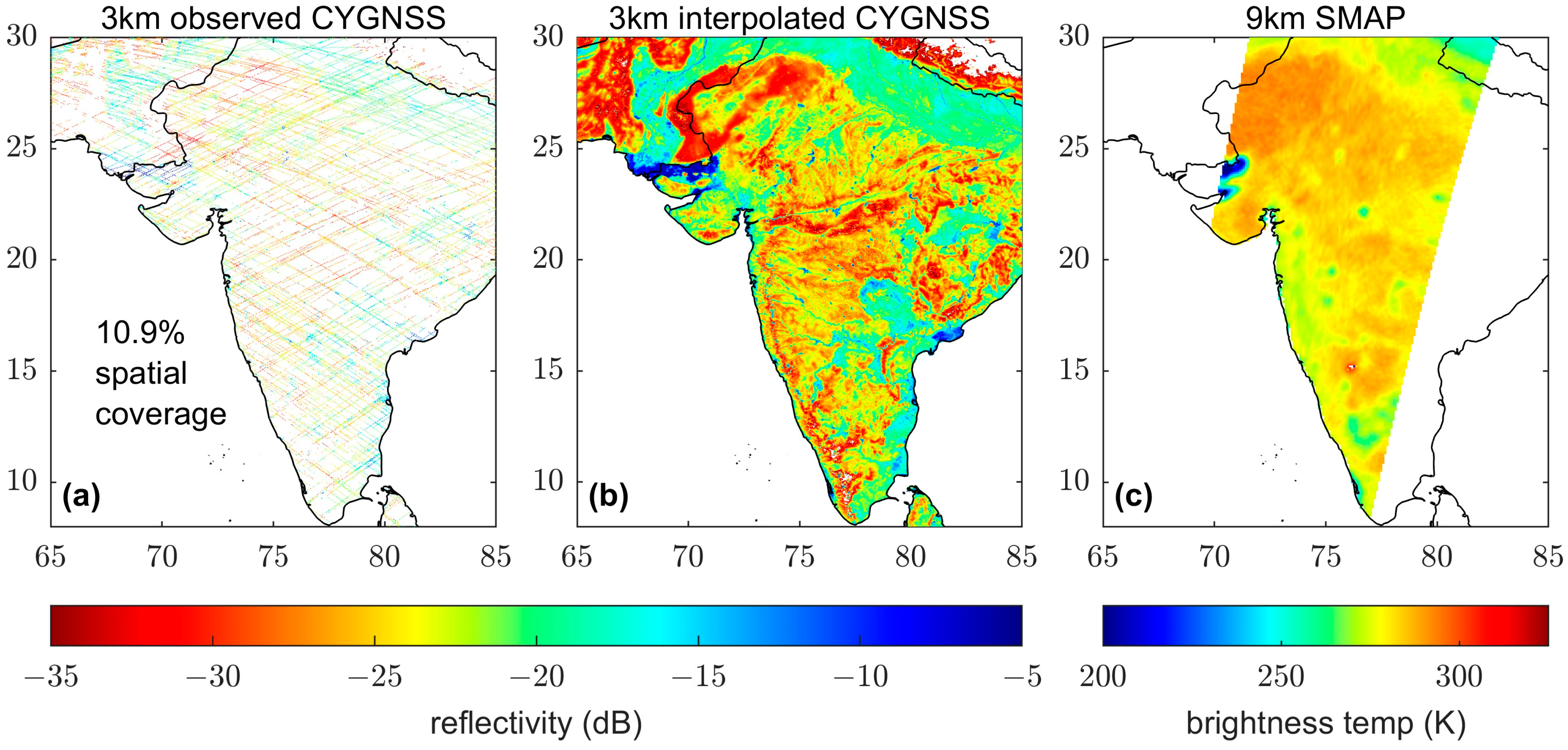
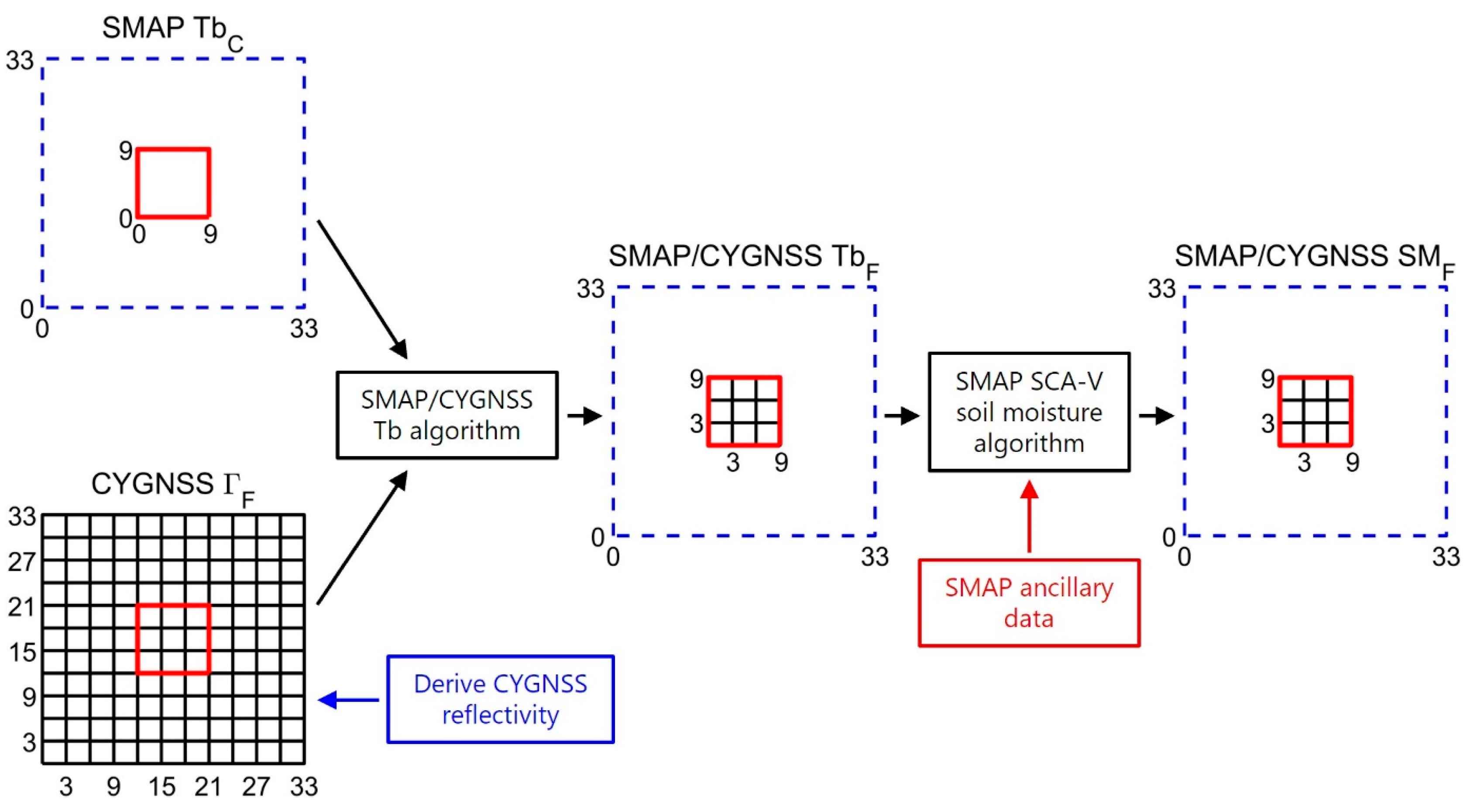
2.1. Deriving CYGNSS Reflectivity

We used version 2.1 Level 1 CYGNSS data for this study [39]. CYGNSS Level 1 data are delay doppler maps, which map the power of the received signal with respect to the doppler shift and time delay [24]. As explained in [23], we used the coherent component of the bistatic radar equation to derive CYGNSS reflectivity (Equation (1)).

$${\Gamma }_s={\displaystyle \frac{P_r{\left[4\pi \left(R_{ts}+R_{sr}\right)\right]}^2}{P_t{G}_t{{\lambda }_t}^2{G}_r}}$$

(1)

Here, ${\Gamma }_s$ is the effective surface reflectivity, $P_r$ is the uncorrected peak power of the CYGNSS DDM (found at the specular reflection point), $R_{ts}$ is the distance from the transmitting antenna to the specular reflection point, $R_{sr}$ is the distance from the specular reflection point to the receiving antenna, $P_t$ is the transmitted power, $G_t$ is the transmitting antenna gain, ${\lambda }_t$ is the transmitted GPS wavelength (0.19 m), and $G_r$ is the receiving antenna gain.

After correcting the peak received power of the CYGNSS DDM for GPS transmit power, antenna gain, and bistatic range [23,27,28], we corrected the effective surface reflectivity for the incidence angle using a modeled, theoretical formula of reflectivity with respect to the incidence angle [32,41]. Finally, we removed all reflectivity values with signal-to-noise ratio values less than 2 dB. The final corrected CYGNSS reflectivity ($\Gamma$) depends only on vegetation effects, surface roughness, and the dielectric constant, which depends on surface soil moisture.

Interpolated CYGNSS Reflectivity

The utility of spatially interpolated CYGNSS soil moisture retrievals depends on choosing an interpolation method that can adequately describe spatial patterns of reflectivity. Due to the high spatial heterogeneity of GNSS-R data relative to the distance between CYGNSS tracks, traditional spatial interpolation techniques do not perform well with CYGNSS data [25], and instead we chose to employ a spatial interpolation technique that was specifically designed for use with GNSS-R data: the Previously Observed Behavior Interpolation (POBI) technique [25]. POBI first calculates the linear relationships of CYGNSS reflectivity, gridded to 3 × 3 km, with its neighbors over time. POBI then uses those linear relationships to predict CYGNSS reflectivity in locations where no observations occurred. POBI is an exact interpolation method, which means that observed reflectivity values are preserved after interpolation. Like all spatial interpolation methods, interpolated grid cells are estimates, though [25] showed that POBI is better at preserving the high spatial heterogeneity characteristic of CYGNSS data than traditional interpolation techniques, with a mean error of 0.17 dB ± 1.96 dB.

2.2. The SMAP/CYGNSS Brightness Temperature Algorithm

After we calculated CYGNSS reflectivity, we then used the SMAP/CYGNSS brightness temperature algorithm to downscale SMAP brightness temperatures [23]. The SMAP/CYGNSS brightness temperature algorithm (Equation (2)) is a slightly modified version of the SMAP active–passive brightness temperature algorithm [6]; because CYGNSS does not include cross-polarization data, there is no cross-polarization term. The SMAP/CYGNSS brightness temperature algorithm (Equation (2)) merges coarse-scale (33 km, gridded at 9 km) SMAP brightness temperatures with fine-scale (3 km) CYGNSS reflectivity values to create fine-scale (3 km) SMAP/CYGNSS brightness temperatures, as shown in Figure 2.

$${Tb}_F={Tb}_C+\left[{Ts}_C·{\beta }_C\right]·\left({\Gamma }_F-{\Gamma }_C\right)$$

(2)

Here, ${Tb}_F$ is fine-scale brightness temperature, ${Tb}_C$ is coarse-scale brightness temperature, and ${Ts}_C$ is coarse-scale surface temperature or effective soil temperature. ${\Gamma }_F$ is fine-scale CYGNSS reflectivity, and ${\Gamma }_C$ is coarse-scale CYGNSS reflectivity. ${\beta }_C$ is the coarse-scale, spatially varying slope of the linear regression between SMAP emissivity and CYGNSS reflectivity time series data. Emissivity is defined as $e={\displaystyle \raisebox{1ex}{${Tb}_C$}\!\left/ \!\raisebox{-1ex}{${Ts}_C$}\right.}$. As described in [23], we used vertically polarized SMAP enhanced 9 km brightness temperatures for the ${Tb}_C$ data [42] and the associated SMAP surface temperatures—Global Modeling and Assimilation Office (GMAO) Goddard Earth Observing System version 5 (GEOS-5) effective soil temperature—for the ${Ts}_C$ data [42]. SMAP emissivity is therefore calculated by dividing the observed SMAP brightness temperature by the modeled GMAO GEOS-5 effective soil temperature [6].

An approximate equilibrium in temperature between the near-surface soil, air, and vegetation at 6 a.m. increases the accuracy of the derived soil moisture [6]. We therefore only used 6 a.m. SMAP brightness temperatures (from descending orbits) in this study. In order to merge the typically asynchronous SMAP and CYGNSS observations, we used temporal merging periods of ±half the time between successive SMAP observations (Figure 3a). The average SMAP repeat period ranges from ~1 to 3 days in low to mid latitudes, so our typical temporal merging periods range from ~1.5 to 5 days, with a median of ~2.5 days. The temporal merging periods of ±half the time between successive SMAP observations allow us to use all available CYGNSS data without reusing any CYGNSS data. However, the relatively long temporal merging periods allow for a greater possibility that SMAP/CYGNSS brightness temperature and soil moisture are not indicative of the soil conditions on the day of the SMAP observation, as discussed in Section 4.2.

The 9 km SMAP enhanced data are gridded at 9 × 9 km, but they have a native resolution of ~33 × 33 km [8]. Both the ${\beta }_C$ and ${\Gamma }_C$ terms were therefore calculated using 33 × 33 km boxes, centered on 9 × 9 km grid cells [7,10]. We calculated ${\Gamma }_C$ by finding the median CYGNSS reflectivity of all ${\Gamma }_F$ values that fell within each 33 × 33 km box within ±half the time between successive SMAP observations (Figure 3b–e). For a more detailed description of the SMAP/CYGNSS brightness temperature algorithm, see [23].

${\beta }_C$ is the scaling factor that determines how much ${Tb}_F$ will vary from ${Tb}_C$. We calculated ${\beta }_C$ using a calibration period of April 2017 through December 2020, and to assure full spatial coverage of the 33 × 33 km boxes while still capturing seasonal variations in soil moisture, we used 45-day intervals to collocate SMAP emissivity and CYGNSS reflectivity. Given the approximately 3.75-year calibration period, we used about 29 collocated SMAP and CYGNSS data points to calculate each ${\beta }_C$ value.

The microwave emissivity of the soil depends on the dielectric constant, which varies based on the water content [43]; SMAP emissivity decreases as soil moisture increases, but CYGNSS reflectivity increases as soil moisture increases. Therefore, ${\beta }_C$ values, and the corresponding correlations of their linear regressions, should theoretically be negative. While most of the SMAP/CYGNSS ${\beta }_C$ values have linear regressions with low, or negative, correlations, arid, forested, and high-topography regions yielded correlations closer to or above zero. We replaced ${\beta }_C$ values with high correlations (R > −0.4) with representative values based on the landcover class. A more detailed description of ${\beta }_C$ and its relationships with soil moisture variance, mean annual precipitation, NDVI, topographic roughness, and landcover class can be found in [23]. A sensitivity analysis evaluating the effect of the uncertainty in each parameter in the SMAP/CYGNSS brightness temperature algorithm can be found in Section 4.2.

Interpolated Versus Observed SMAP/CYGNSS Brightness Temperatures

There are two major differences in the calculated 3 km SMAP/CYGNSS observed brightness temperature and interpolated brightness temperature. First, the interpolated brightness temperature has significantly better daily spatial coverage, which leads to significantly denser time series data (Figure 3a). Second, ${\Gamma }_C$ values calculated using interpolated CYGNSS data are much more representative of the spatial heterogeneity of their 33 km boxes than ${\Gamma }_C$ values calculated using observed CYGNSS data (Figure 3b–e). The 3 km interpolated SMAP/CYGNSS brightness temperatures should therefore include fewer outliers produced from non-representative ${\Gamma }_C$ values.

A difference also exists in how we calculated interpolated and observed SMAP/CYGNSS brightness temperature. In order to conserve energy in the brightness temperature space, similarly to the SMAP active–passive brightness temperature algorithm [10], we applied a bias correction to the 3 km interpolated SMAP/CYGNSS brightness temperatures. We calculated bias by (1) calculating the mean of all 3 km SMAP/CYGNSS brightness temperatures within the 33 km box associated with each 9 km grid cell, and (2) subtracting the mean SMAP/CYGNSS brightness temperature from the 9 km SMAP brightness temperature. We then subtracted the bias from all 3 km SMAP/CYGNSS brightness temperatures within the 9 km grid cell. We did not apply a bias correction to the 3 km observed SMAP/CYGNSS brightness temperatures due to the incomplete spatial coverage of the 33 km boxes associated with the 9 km grid cells (as seen in Figure 3b). The incomplete spatial coverage makes the calculated mean brightness temperature of each 33 km box non-representative of its true spatial heterogeneity, which makes conserving energy in the brightness temperature space implausible.

2.3. Calculating SMAP/CYGNSS Soil Moisture

After calculating 3 km SMAP/CYGNSS brightness temperature, we calculated soil moisture using the SMAP SCA-V soil moisture algorithm. The SCA-V algorithm is a version of the tau-omega model, which uses effective soil temperature, surface roughness, soil texture properties, and vegetation properties to convert the brightness temperature to a dielectric constant [6,44] and then uses the Mironov dielectric mixing model [45] to determine the soil moisture.

When applying the SMAP SCA-V algorithm, we used 3 km SMAP ancillary data whenever possible. We defined the vegetation parameter (b), stem factor, roughness parameter (h), and single scatter albedo (ω) using 3 km MODIS landcover class [46] and the SMAP lookup table of algorithm parameters by landcover class [44]. We used SMAP ancillary 3 km soil properties (percent clay, percent sand, and bulk density), which were derived from SoilGrid250m [47]. These parameters are all static. We calculated the vegetation optical depth (τ) by converting day-of-year 3 km NDVI values [46] to vegetation water content (VWC) [48] and then multiplying by b $\left(\tau =VWC·b\right)$ [44]. We used 9 km SMAP surface temperature (GMAO GEOS-5 effective soil temperature) [42], as 3 km surface temperature is not provided in SMAP data. A sensitivity analysis evaluating the effect of the uncertainty in each parameter in the SMAP SCA-V algorithm can be found in Section 4.2.

As suggested in [6], we set upper and lower bounds for soil moisture based on porosity and residual water content, respectively. For each 3 × 3 km grid cell, we used porosity, based on soil bulk density, to determine a maximum soil moisture limit [47]. We also determined a minimum soil moisture limit for each 3 × 3 km grid cell, based on residual water content, which we calculated using the Rosetta Model [49] and the soil texture class.

3. Results

We first discuss the spatial heterogeneity, spatial detail, spatial coverage, and repeat period of 3 km SMAP/CYGNSS soil moisture. We then present SMAP/CYGNSS soil moisture validation results.

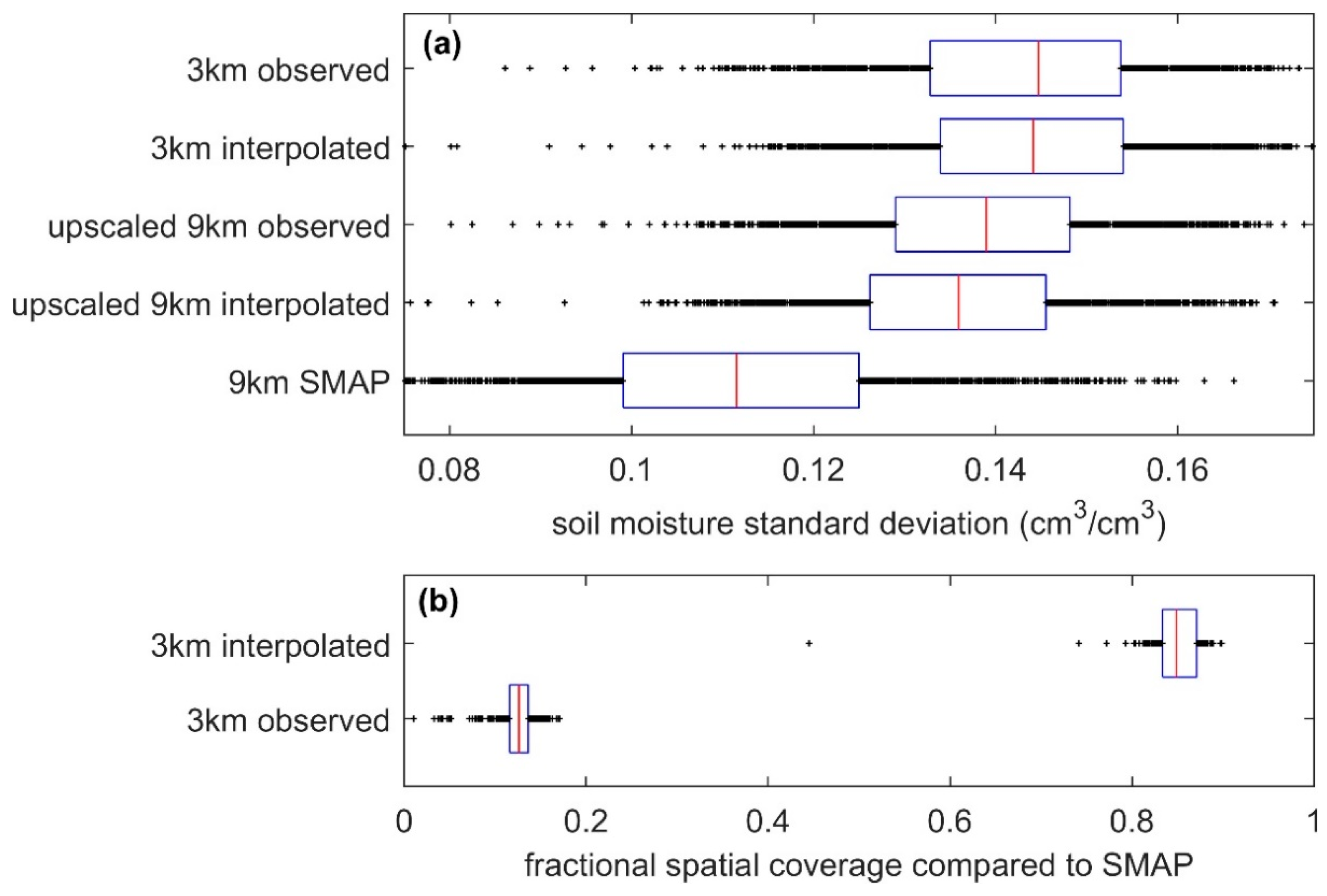
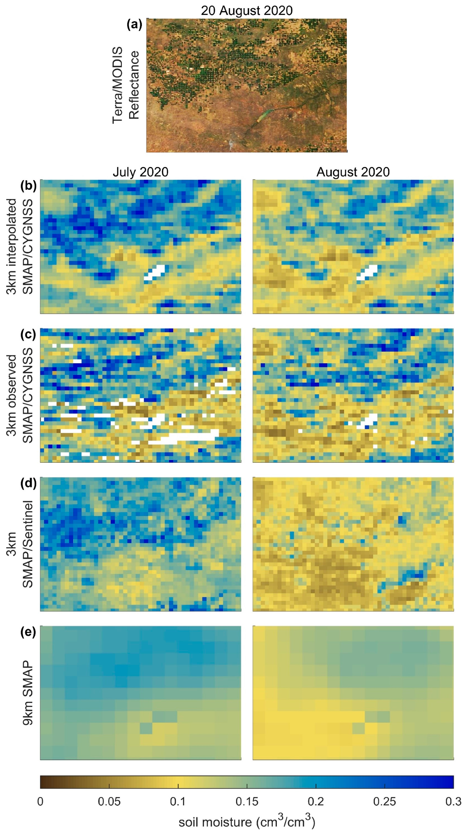
3.1. Spatial Heterogeneity and Spatial Detail

A downscaled soil moisture product should exhibit greater spatial heterogeneity than the original soil moisture product. We therefore expect 3 km SMAP/CYGNSS soil moisture to be more spatially heterogeneous than 9 km SMAP soil moisture. Additionally, we expect SMAP/CYGNSS soil moisture upscaled to 9 km to be more spatially heterogeneous than 9 km SMAP soil moisture because the native resolution of 9 km SMAP enhanced soil moisture is ~33 km [8]. We estimated spatial heterogeneity by calculating the standard deviation of daily soil moisture over the continental United States (US) (Figure 4a). SMAP/CYGNSS soil moisture upscaled to 9 km is approximately 22–25% more spatially heterogeneous than 9 km SMAP soil moisture, and 3 km SMAP/CYGNSS soil moisture is approximately 30% more spatially heterogeneous than 9 km SMAP soil moisture. The increased spatial heterogeneity of SMAP/CYGNSS soil moisture, compared to 9 km SMAP soil moisture, indicates a successful downscaling algorithm and suggests that SMAP/CYGNSS soil moisture should include more spatial detail than 9 km SMAP soil moisture.

Both 3 km interpolated and observed SMAP/CYGNSS soil moisture show improved spatial detail, compared to 9 km SMAP soil moisture, and capture expected soil moisture patterns on the landscape. As an example, we examine the soil moisture in both July 2020 and August 2020 in an approximately 150 km × 100 km region of northwest Texas, USA (Figure 5). Monthly soil moisture maps for 3 km interpolated and observed SMAP/CYGNSS, 3 km SMAP/Sentinel, and 9 km SMAP are compared to a Terra/MODIS reflectance image of the same region on 20 August 2020. We aggregated data over monthly periods to ensure full spatial coverage for both 3 km observed SMAP/CYGNSS and 3 km SMAP/Sentinel soil moisture and to better depict the differences in the 3 km and 9 km soil moisture patterns. Enhanced spatial detail is evident for all 3 km soil moisture maps, compared to 9 km SMAP soil moisture. Notably, 3 km interpolated SMAP/CYGNSS soil moisture shows remarkable similarities when compared to the Terra/MODIS reflectance image, clearly delineating regions of higher soil moisture over irrigated cropland and regions of lower soil moisture in adjacent non-agricultural areas. Additionally, while all the soil moisture maps capture a dry-down from July to August, 3 km interpolated SMAP/CYGNSS soil moisture captures the decrease in soil moisture primarily over the irrigated cropland, while many of the non-agricultural areas display minimal change.

3.2. Spatial Coverage and Repeat Period

3 km interpolated SMAP/CYGNSS soil moisture has nearly identical daily spatial coverage as 9 km SMAP soil moisture within the latitudinal range of ±37°, except over densely forested areas and mountainous terrain (Figure 6). However, 3 km observed SMAP/CYGNSS soil moisture has somewhat poor daily spatial coverage (Figure 6). On average, 3 km interpolated SMAP/CYGNSS soil moisture covers 85.0% of the spatial area that SMAP observes, and 3 km observed SMAP/CYGNSS soil moisture covers 12.4% of the spatial area that SMAP observes (Figure 4b), within ±37°. Because 3 km interpolated SMAP/CYGNSS soil moisture matches the daily spatial coverage of SMAP soil moisture, the repeat period of 3 km interpolated SMAP/CYGNSS soil moisture also matches the SMAP repeat period of approximately 2–3 days, except over densely forested areas and mountainous terrain. Conversely, 3 km observed SMAP/CYGNSS soil moisture has a longer repeat period than SMAP. The exact repeat period of 3 km observed SMAP/CYGNSS soil moisture is difficult to determine due to the pseudo-random, Signals-of-Opportunity retrieval pattern of observed CYGNSS data. However, based on the average daily spatial coverage of 12.4%, compared to SMAP soil moisture, we estimate that the repeat period of 3 km observed SMAP/CYGNSS soil moisture is ~16–24 days.

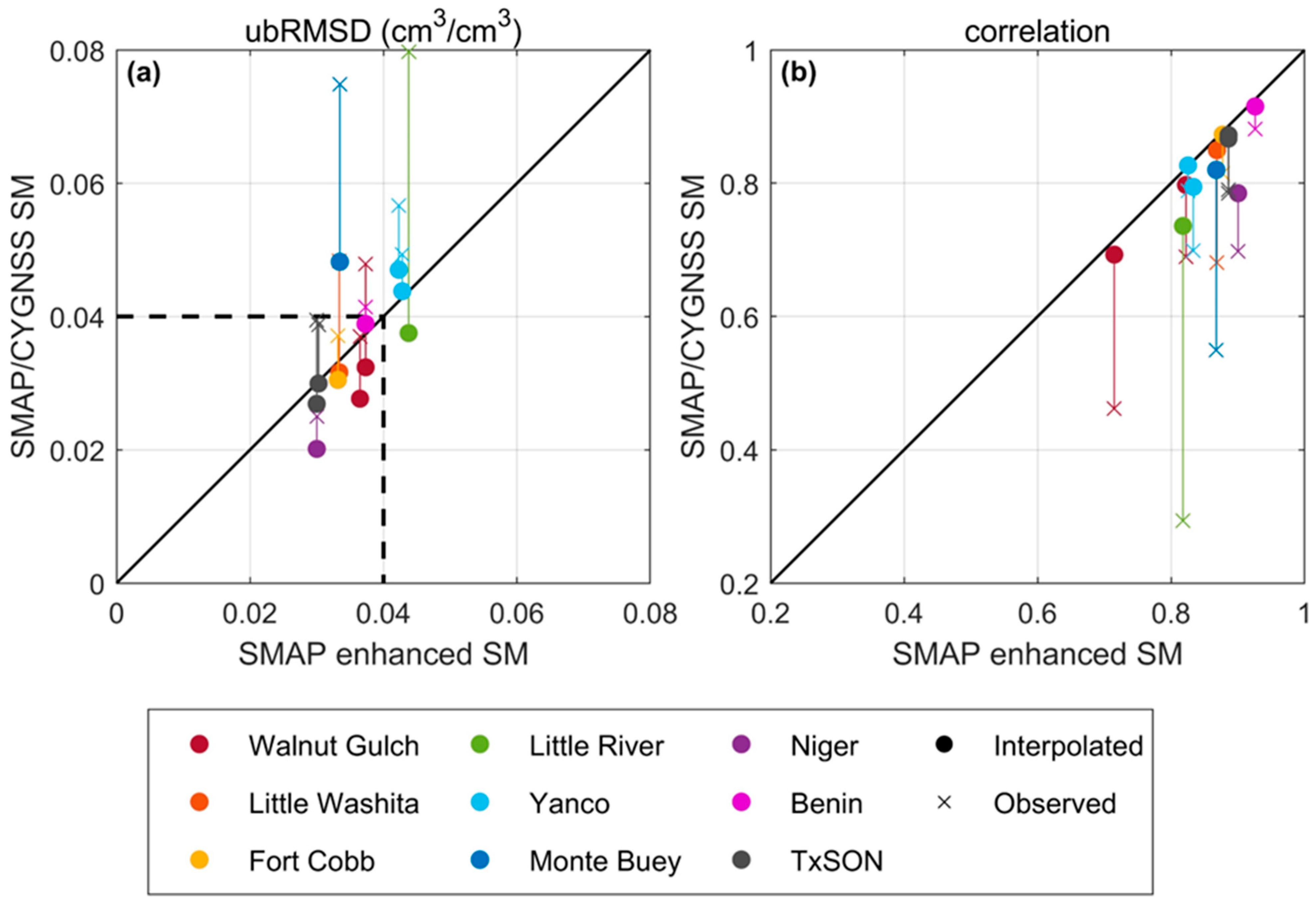
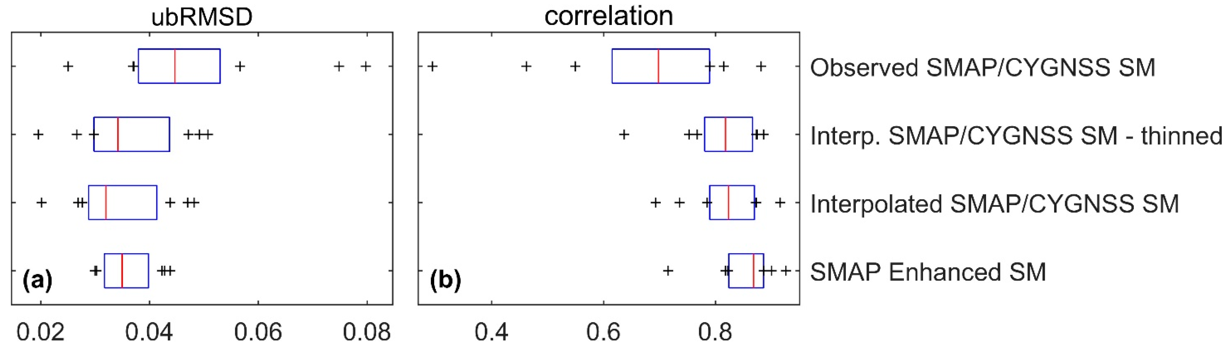
3.3. Validating SMAP/CYGNSS Soil Moisture with SMAP Core Validation Sites

SMAP uses a variety of core validation sites (CVSs) to calibrate and validate SMAP soil moisture products. Each of these sites contains multiple in situ sensors, and both weighted and linear average soil moisture are reported for 3 km, 9 km, or 36 km spatial resolutions, depending on the site [46]. The average soil moisture values reported at these sites are theoretically more representative of the true soil moisture than a single soil moisture probe would be [52].

We validated SMAP/CYGNSS soil moisture using all 9 km SMAP CVSs within ±38° latitude and a time period of April 2017 through March 2021. Details regarding the SMAP CVSs used in this validation are included in the Supplementary Material (Table S1). We chose to only use 9 km SMAP CVSs due to the limited time series availability of 3 km SMAP CVSs; publicly available 3 km SMAP CVS data only span from April 2015 to July 2015. We used the weighted average soil moisture from each SMAP CVS [46,53], and we upscaled 3 km SMAP/CYGNSS soil moisture to 9 km using a linear average.

Interpolated SMAP/CYGNSS soil moisture performs similarly to 9 km SMAP enhanced soil moisture at the 9 km CVSs used in this study (Figure 7 and Table S1). Upscaled interpolated SMAP/CYGNSS soil moisture has an average correlation of 0.82 and an average ubRMSD of 0.035 cm³/cm³, whereas 9 km SMAP soil moisture has an average correlation of 0.85 and an average ubRMSD of 0.036 cm³/cm³. Interpolated SMAP/CYGNSS soil moisture usually performs best at CVSs where the SMAP soil moisture also performs well, in terms of both ubRMSD and correlation (Figure 7). For example, the sites with the lowest SMAP ubRMSDs (Niger and TxSON) also have the lowest SMAP/CYGNSS ubRMSDs, and both datasets have the highest correlation at the same site (Benin). Because SMAP brightness temperature directly affects SMAP/CYGNSS soil moisture, this is expected.

In contrast, observed SMAP/CYGNSS soil moisture performs substantially worse than 9 km enhanced SMAP soil moisture at the 9 km SMAP CVSs used in this study (Figure 7 and Table S1). Upscaled observed SMAP/CYGNSS soil moisture has an average correlation of 0.68 and an average ubRMSD of 0.048 cm³/cm³. To determine whether the inferior performance of observed SMAP/CYGNSS soil moisture was due to the lower sampling rate (every ~16–24 days instead of every ~2–3 days), we also calculated 9 km SMAP CVS statistics for interpolated SMAP/CYGNSS soil moisture thinned to only include data on the same days as observed SMAP/CYGNSS soil moisture. The CVS statistics for the thinned and original (not thinned) interpolated SMAP/CYGNSS soil moisture were very similar, on average (Figure 8). This shows that the relatively poor performance of observed SMAP/CYGNSS soil moisture is not due to the lower sampling rate.

To provide more context for the performance of 3 km SMAP/CYGNSS soil moisture, we provide time series and scatter plots from the TxSON CVS (Figure 9). Time series and scatter plots for the remaining CVSs used in this study are included in the Supplementary Material (Figures S1–S11). Like SMAP soil moisture, both observed and interpolated SMAP/CYGNSS soil moisture capture a sequence of dry-downs and show the dry (~July–December) versus wet (~January–June) season at the TxSON CVS. Additionally, the SMAP/CYGNSS soil moisture range is very similar to the SMAP soil moisture range. Finally, the comparison of observed and interpolated SMAP/CYGNSS soil moisture at the TxSON CVS demonstrates both the reduced amount of observed SMAP/CYGNSS time series data and the increase in noise and outliers for observed SMAP/CYGNSS soil moisture. The decreased accuracy of observed SMAP/CYGNSS soil moisture, compared to interpolated SMAP/CYGNSS soil moisture, is likely due to the poor spatial representation of ${\Gamma }_C$ values in the SMAP/CYGNSS brightness temperature algorithm, as explained in the Interpolated Versus Observed SMAP/CYGNSS Brightness Temperatures Section.

3.4. Validating SMAP/CYGNSS Soil Moisture with Sparse Networks

Sparse networks, or networks of in situ soil moisture sensors, report soil moisture measured at a series of individual point locations. We expect SMAP/CYGNSS soil moisture validation statistics to be worse at sparse network sites, compared to SMAP CVSs, for a few reasons. First, in almost all cases, there is only a single soil moisture sensor per 3 km or 9 km EASE-2 grid cell. Therefore, the upscaled, average soil moisture provided at SMAP CVSs is more representative of the larger area that the satellites view than the soil moisture provided by individual sparse network sites. Second, the noise in the CYGNSS data will be more apparent in the 3 km SMAP/CYGNSS soil moisture than the upscaled 9 km SMAP/CYGNSS soil moisture. Finally, sparse network data are typically subject to less quality control than data collected at SMAP CVSs.

We validated 3 km SMAP/CYGNSS soil moisture using four sparse networks: the US Department of Agriculture Soil Climate Analysis Network (SCAN), the National Oceanic and Atmospheric Administration US Climate Reference Network (USCRN), the Trans-African Hydro-Meteorological Observatory (TAHMO), and OzNet (

Table 1. Sparse network information and validation statistics for 3 km observed and interpolated SMAP/CYGNSS soil moisture. All data retrieved from the International Soil Moisture Network [54].

Sparse Network	Location	Sensor Depth (cm)	Number of Sites	Avg. ubRMSD (cm3/cm3)		Avg. Correlation
				Obs.	Interp.	Obs.	Interp.
SCAN 1	United States	5	35	0.060	0.050	0.54	0.63
USCRN 2	United States	5	23	0.055	0.044	0.57	0.65
OzNet 3	Southeast Australia	0–5	9	0.073	0.063	0.61	0.69
TAHMO 4	Central Africa (Ghana and Kenya)	10	17	0.059	0.058	0.74	0.75
		All:	84	0.060	0.051	0.60	0.67

¹ SCAN—Soil Climate Analysis Network [55]. ² USCRN—United States Climate Reference Network [56]. ³ OzNet [57]. ⁴ TAHMO—Trans-African Hydro-Meteorological Observatory.

). We manually chose sites from each sparse network with hydrologically reasonable soil moisture time series and substantial temporal overlap (at least six sequential months) between the in situ and SMAP/CYGNSS data. We did not include any sites with static or zero-value in situ soil moisture data or with limited observed SMAP/CYGNSS soil moisture data. We also did not include sites for which 3 km SMAP/CYGNSS soil moisture maintained a maximum soil moisture value for extended periods, likely indicating the nearby presence of standing water or saturated soil. We performed all sparse network analyses using a validation period of April 2017 through December 2021.

The average ubRMSD of 3 km interpolated SMAP/CYGNSS soil moisture at the sparse network sites used in this study is 0.051 cm³/cm³, and the average correlation is 0.67 (Table 1). In comparison, the average ubRMSD of 9 km SMAP enhanced soil moisture at the sparse network sites is 0.048 cm³/cm³, and the average correlation is 0.73. The average ubRMSD of 3 km observed SMAP/CYGNSS soil moisture at the sparse network sites is 0.060 cm³/cm³, and the average correlation is 0.60 (Table 1). Thus, the results from the sparse network validation are consistent with the results from the SMAP CVS validation; interpolated SMAP/CYGNSS soil moisture performs similarly to 9 km SMAP soil moisture, and interpolated SMAP/CYGNSS soil moisture outperforms observed SMAP/CYGNSS soil moisture.

4. Discussion

4.1. Comparison with Other Fine-Resolution Soil Moistures

To provide perspective on the accuracy and utility of the 3 km SMAP/CYGNSS soil moisture datasets, we compared the validation statistics discussed above with 3 km SMAP active–passive [10] and 3 km SMAP/Sentinel [7] validation statistics (

Table 2. A comparison of 3 km soil moisture validation statistics. SMAP active-passive data from [10]. SMAP/Sentinel data from [7]. * Sparse network correlation results were not reported for the SMAP active–passive product.

	SMAP CVS ubRMSD (cm3/cm3)	SMAP CVS Correlation	Sparse Network ubRMSD (cm3/cm3)	Sparse Network Correlation
Observed SMAP/CYGNSS	0.048	0.68	0.060	0.60
Interpolated SMAP/CYGNSS	0.035	0.82	0.051	0.67
SMAP active–passive	0.039	0.66	~0.055	n/a *
SMAP/Sentinel	0.036	0.83	0.050	0.59

). For a comparison at 9 km SMAP CVSs, we are reporting 9 km SMAP active–passive and upscaled 3 km SMAP/Sentinel results. For a comparison of sparse networks, we are reporting 3 km SMAP active–passive and 3 km SMAP/Sentinel results.

There is some overlap in the CVSs and sparse networks used to calculate the validation statistics for all three datasets. However, the time periods are different. SMAP active–passive statistics used soil moisture data from April 2015 to July 2015; SMAP-Sentinel statistics used soil moisture data from April 2015 to October 2018; and SMAP/CYGNSS statistics used soil moisture data from April 2017 to December 2021. While we can conclude that observed SMAP/CYGNSS soil moisture performs worse than interpolated SMAP/CYGNSS soil moisture, the differences in statistics between interpolated SMAP/CYGNSS, SMAP active–passive, and SMAP/Sentinel soil moisture are too small to make any confident claims about their relative performance. We posit that, based on the similarity of the validation statistics, 3 km interpolated SMAP/CYGNSS soil moisture has effectively equal accuracy to 3 km SMAP/Sentinel soil moisture. However, the shorter repeat period of 3 km interpolated SMAP/CYGNSS soil moisture may make it more useful for some hydrologic and climatic applications.

4.2. Uncertainties and Sensitivity Analysis

Uncertainties in 3 km SMAP/CYGNSS soil moisture arise from uncertainties in (1) SMAP brightness temperature, (2) SMAP ancillary data, (3) CYGNSS reflectivity data, and (4) SMAP/CYGNSS ${\beta }_C$ values. The uncertainties associated with SMAP brightness temperature and SMAP ancillary data were estimated by the SMAP team [44].

CYGNSS reflectivity data include significant uncertainty, which propagates into SMAP/CYGNSS soil moisture. First, CYGNSS data are not necessarily optimized over land, as CYGNSS data are calibrated to optimize retrievals over the ocean [58]. Second, there is uncertainty regarding some of the ancillary variables in the bistatic radar equation. Most significantly, the GPS effective isotropic radiated power (EIRP) for the v2.1 data is estimated from a lookup table and does not consider variations in transmit power due to GPS flex power modes [58]. Finally, the following assumptions introduce uncertainty into the CYGNSS reflectivity values: (1) the assumption that CYGNSS reflectivity retrievals over land are completely coherent and (2) the assumption that CYGNSS reflectivity values grid to 3 × 3 km, which does not account for the elongated footprint of CYGNSS observations.

We estimated a bulk uncertainty in CYGNSS reflectivity values by calculating the standard deviation of reflectivity over each 3 km grid cell using all available CYGNSS data from 2017 to 2021. To remove the expected fluctuations associated with changing soil moisture, we only included CYGNSS observations that were concurrent with SMAP soil moisture measurements within ±0.02 cm³/cm³ of the mean soil moisture for each 3 km grid cell. The peak of the resulting standard deviation distribution indicates that a reasonable CYGNSS reflectivity uncertainty over land is approximately ±1.75 dB. Additionally, the standard deviation of the interpolated CYGNSS reflectivity error calculated using the POBI algorithm is ~2 dB [25].

SMAP/CYGNSS ${\beta }_C$ values also have the potential to propagate significant uncertainty to SMAP/CYGNSS soil moisture. When the linear regressions between SMAP emissivity and CYGNSS reflectivity observations are poorly correlated, ${\beta }_C$ values might be inaccurate or even unrealistic. While we removed potentially inaccurate SMAP/CYGNSS ${\beta }_C$ values by replacing poorly correlated ${\beta }_C$ values with representative values, as explained in Section 2.2 and [23], ${\beta }_C$ values still include uncertainty. Following the SMAP/Sentinel precedent [59], we estimate that a nominal uncertainty in ${\beta }_C$ is 20%.

To determine how estimated uncertainty in SMAP brightness temperature, SMAP ancillary data, CYGNSS data, and SMAP/CYGNSS ${\beta }_C$ values affect 3 km SMAP/CYGNSS soil moisture, we performed a sensitivity analysis, varying one parameter at a time. This sensitivity analysis is equivalent to the SMAP passive soil moisture sensitivity analysis [44]. We used a test region of the continental US (25–38°N, 75–125°E) and a test period of 2020 for this analysis, which amounts to approximately 70 million test cases over a diverse landscape. We used normally distributed random number arrays to vary each parameter by its estimated uncertainty (

Table 3. 3 km SMAP/CYGNSS soil moisture sensitivity analysis. Uncertainty estimates for each parameter in the SMAP/CYGNSS brightness temperature algorithm and the SMAP SCA-V soil moisture algorithm that contributes uncertainty to 3 km SMAP/CYGNSS soil moisture and the effect on 3 km SMAP/CYGNSS soil moisture by varying one parameter at a time. Abbreviations: SM—soil moisture, SSA—single scatter albedo.

Uncertainty Parameter	Uncertainty Estimate	Interpolated SM RMSE (cm3/cm3)	Observed SM RMSE (cm3/cm3)
Veg. Opt. Depth	5%	0.0065	0.0068
% clay	5%	0.0025	0.0027
Roughness	5%	0.0009	0.0009
SSA	5%	0.0077	0.0072
9 km Tb	1.3 K	0.0136	0.0131
Surf. Temp.	2 K	0.0184	0.0176
SMAP/CYG ${\beta }_C$	20%	0.0151	0.0174
CYGNSS	2 dB	0.0619	0.0664

) for the entire region and period and then recalculated the soil moisture. We then compared the sensitivity analysis soil moisture with the original 3 km SMAP/CYGNSS soil moisture using RMSE. The results are displayed in Table 3 and Figure 10.

CYGNSS reflectivity uncertainty accounts for the greatest uncertainty in SMAP/CYGNSS soil moisture, based on our sensitivity analysis and uncertainty estimates. However, because the interpolated soil moisture RMSE based on uncertainty in CYGNSS reflectivity from the sensitivity analysis (0.062 cm³/cm³) is notably higher than the interpolated SMAP/CYGNSS CVS validation average ubRMSD (0.035 cm³/cm³), the CYGNSS reflectivity uncertainty estimate of 2 dB may be too high. Figure 10 shows how varying the CYGNSS reflectivity uncertainty estimates affects 3 km SMAP/CYGNSS soil moisture, compared to the rest of the uncertainty analysis parameters. In order to meet the SMAP accuracy requirements of 0.04 cm³/cm³, CYGNSS reflectivity uncertainty would need to be ~1 dB or less. Presumably, the CYGNSS reflectivity uncertainty at the SMAP CVSs within ±38° is <1 dB.

Surface temperature uncertainty accounts for the second greatest uncertainty in SMAP/CYGNSS soil moisture. This is likely due to the coarse spatial resolution of the GMAO GEOS-5 effective soil temperature, which is used as surface temperature in the SMAP brightness temperature and soil moisture algorithms [6]. 9 km SMAP surface temperature is gridded at 9 × 9 km, but the resolution of the GMAO GEOS-5 effective soil temperature is 0.25° × 0.3125° [60]. While such a coarse resolution surface temperature cannot capture fine-scale changes, we chose to use the 9 km surface temperature provided by SMAP for simplicity of data processing and to provide a more direct comparison of SMAP/CYGNSS soil moisture with SMAP and SMAP/Sentinel soil moisture.

The SMAP/CYGNSS brightness temperature algorithm also introduces uncertainty due to the relatively long temporal merging periods, which may allow for soil moisture changes between a SMAP and CYGNSS observation, especially if precipitation occurs between the merged observations. Consequently, 3 km SMAP/CYGNSS brightness temperature and soil moisture values might not always be representative of the conditions on the day of the SMAP observation. The SMAP/CYGNSS temporal merging periods typically range from ~1.5 to 5 days. Because the merged CYGNSS observation(s) might have occurred at any point during those ~1.5–5 days, creating a precipitation flag is somewhat arbitrary. We therefore chose not to include a SMAP/CYGNSS precipitation flag. However, we include 9 km SMAP surface flags [42] with our 3 km SMAP/CYGNSS soil moisture data, interpolated to 3 × 3 km.

5. Conclusions

We downscaled SMAP brightness temperatures to 3 km [23] using both observed and spatially interpolated [25] CYGNSS reflectivity, then used the SMAP SCA-V algorithm [6] and SMAP ancillary data to calculate 3 km SMAP/CYGNSS soil moisture. 3 km interpolated SMAP/CYGNSS soil moisture matches the SMAP repeat period of ~2–3 days, except in densely forested and mountainous regions, whereas the average repeat period for observed SMAP/CYGNSS soil moisture is ~16–24 days. Both 3 km interpolated and observed SMAP/CYGNSS soil moistures have increased spatial heterogeneity and show improved spatial detail when compared to 9 km SMAP soil moisture and capture expected soil moisture patterns on the landscape.

Interpolated SMAP/CYGNSS soil moisture performs similarly to 9 km SMAP soil moisture at both SMAP 9 km CVSs and sparse networks. Additionally, 3 km interpolated SMAP/CYGNSS soil moisture has effectively equal accuracy to 3 km SMAP/Sentinel soil moisture and a shorter repeat period. However, observed SMAP/CYGNSS soil moisture performs worse than both 9 km SMAP soil moisture and 3 km SMAP/Sentinel soil moisture. Using all SMAP 9 km CVSs within ±38° latitude, upscaled interpolated SMAP/CYGNSS soil moisture has an average ubRMSD of 0.035 cm³/cm³ and an average correlation of 0.82, whereas upscaled observed SMAP/CYGNSS soil moisture has an average ubRMSD of 0.048 cm³/cm³ and an average correlation of 0.68. Using four different sparse networks on three continents, 3 km interpolated SMAP/CYGNSS soil moisture has an average ubRMSD of 0.051 cm³/cm³ and an average correlation of 0.67. 3 km observed SMAP/CYGNSS soil moisture has an average ubRSMD of 0.060 cm³/cm³ and an average correlation of 0.60 at the sparse networks used in this study. A sensitivity analysis demonstrates that CYGNSS reflectivity is likely most responsible for the uncertainty in SMAP/CYGNSS soil moisture, followed by surface temperature and SMAP/CYGNSS ${\beta }_C$.

The success of 3 km SMAP/CYGNSS soil moisture demonstrates that GNSS-R observations are effective for downscaling soil moisture. Additionally, the higher accuracy of interpolated SMAP/CYGNSS soil moisture, compared to observed SMAP/CYGNSS soil moisture, implies that future GNSS-R missions, with larger constellations and the capacity to retrieve more signals at once (e.g., [61,62]), will be increasingly valuable for downscaling soil moisture data.

References

1. Peng, J.; Albergel, C.; Balenzano, A.; Brocca, L.; Cartus, O.; Cosh, M.H.; Crow, W.T.; Dabrowska-Zielinska, K.; Dadson, S.; Davidson, M.W.J.; et al. A Roadmap for High-Resolution Satellite Soil Moisture Applications—Confronting Product Characteristics with User Requirements. Remote Sens. Environ. 2021, 252, 112162. [Google Scholar] [CrossRef]
2. Kerr, Y.H.; Waldteufel, P.; Wigneron, J.; Delwart, S.; Cabot, F.; Boutin, J.; Escorihuela, M.J.; Font, J.; Reul, N.; Gruhier, C.; et al. The SMOS Mission: New Tool for Monitoring Key Elements of the Global Water Cycle. Proc. IEEE 2010, 98, 666–687. [Google Scholar] [CrossRef]
3. Njoku, E.G.; Jackson, T.J.; Lakshmi, V.; Chan, T.K.; Nghiem, S.V. Soil Moisture Retrieval from AMSR-E. IEEE Trans. Geosci. Remote Sens. 2003, 41, 215–229. [Google Scholar] [CrossRef]
4. Torres, R.; Snoeij, P.; Geudtner, D.; Bibby, D.; Davidson, M.; Attema, E.; Potin, P.; Rommen, B.; Floury, N.; Brown, M.; et al. Remote Sensing of Environment GMES Sentinel-1 Mission. Remote Sens. Environ. 2012, 120, 9–24. [Google Scholar] [CrossRef]
5. Kellogg, K.; Rosen, P.; Barela, P.; Hoffman, P.; Edelstein, W.; Standley, S.; Dunn, C.; Guerrero, A.M.; Harinath, N.; Shaffer, S.; et al. NASA-ISRO Synthetic Aperture Radar (NISAR) Mission. In Proceedings of the IEEE Aerospace Conference, Big Sky, Montana, USA, 7–14 March 2020. [Google Scholar]
6. Entekhabi, D.; Yueh, S.; O’Neill, P.E.; Kellogg, K.H.; Allen, A.; Bindlish, R.; Brown, M.; Chan, S.; Colliander, A.; Crow, W.T.; et al. SMAP Handbook: Soil Moisture Active Passive: Mapping Soil Moisture and Freeze/Thaw from Space; Jet Propulsion Laboratory: Pasadena, CA, USA, 2014. [Google Scholar]
7. Das, N.; Entekhabi, D.; Dunbar, R.S.; Chaubell, M.J.; Colliander, A.; Yueh, S.; Jagdhuber, T.; Chen, F.; Crow, W.; O’Neill, P.E.; et al. The SMAP and Copernicus Sentinel 1A/B Microwave Active-Passive High Resolution Surface Soil Moisture Product. Remote Sens. Environ. 2019, 233, 111380. [Google Scholar] [CrossRef]
8. Chan, S.K.; Bindlish, R.; Neill, P.O.; Jackson, T.; Njoku, E.; Dunbar, S.; Chaubell, J.; Piepmeier, J.; Yueh, S.; Entekhabi, D.; et al. Development and Assessment of the SMAP Enhanced Passive Soil Moisture Product. Remote Sens. Environ. 2018, 204, 931–941. [Google Scholar] [CrossRef]
9. Peng, J.; Loew, A.; Merlin, O.; Verhoest, N.E.C. A Review of Spatial Downscaling of Satellite Remotely Sensed Soil Moisture. Rev. Geophys. 2017, 55, 341–366. [Google Scholar] [CrossRef]
10. Das, N.; Entekhabi, D.; Dunbar, R.S.; Colliander, A.; Chen, F.; Crow, W.; Jackson, T.J.; Berg, A.; Bosch, D.D.; Caldwell, T.; et al. The SMAP Mission Combined Active-Passive Soil Moisture Product at 9 km and 3 km Spatial Resolutions. Remote Sens. Environ. 2018, 211, 204–217. [Google Scholar] [CrossRef]
11. Wei, Z.; Meng, Y.; Zhang, W.; Peng, J.; Meng, L. Downscaling SMAP Soil Moisture Estimation with Gradient Boosting Decision Tree Regression over the Tibetan Plateau. Remote Sens. Environ. 2019, 225, 30–44. [Google Scholar] [CrossRef]
12. Zhao, W.; Sánchez, N.; Lu, H.; Li, A. A Spatial Downscaling Approach for the SMAP Passive Surface Soil Moisture Product Using Random Forest Regression. J. Hydrol. 2018, 563, 1009–1024. [Google Scholar] [CrossRef]
13. Abbaszadeh, P.; Moradkhani, H.; Zhan, X. Downscaling SMAP Radiometer Soil Moisture Over the CONUS Using an Ensemble Learning Method. Water Resour. Res. 2019, 55, 324–344. [Google Scholar] [CrossRef]
14. Xu, M.; Yao, N.; Yang, H.; Xu, J.; Hu, A.; Gustavo Goncalves De Goncalves, L.; Liu, G. Downscaling SMAP Soil Moisture Using a Wide & Deep Learning Method over the Continental United States. J. Hydrol. 2022, 609, 127784. [Google Scholar] [CrossRef]
15. Fang, B.; Lakshmi, V.; Bindlish, R.; Jackson, T.J. Downscaling of SMAP Soil Moisture Using Land Surface Temperature and Vegetation Data. Vadose Zone J. 2018, 17, 1–15. [Google Scholar] [CrossRef]
16. Dandridge, C.; Fang, B.; Lakshmi, V. Downscaling of SMAP Soil Moisture in the Lower Mekong River Basin. Water 2019, 12, 56. [Google Scholar] [CrossRef]
17. Fang, B.; Lakshmi, V.; Cosh, M.; Liu, P.-W.; Bindlish, R.; Jackson, T.J. A Global 1-km Downscaled SMAP Soil Moisture Product Based on Thermal Inertia Theory. Vadose Zone J. 2022, 21, e20182. [Google Scholar] [CrossRef]
18. Ojha, N.; Merlin, O.; Molero, B.; Suere, C.; Olivera-Guerra, L.; Ait Hssaine, B.; Amazirh, A.; Al Bitar, A.; Escorihuela, M.; Er-Raki, S. Stepwise Disaggregation of SMAP Soil Moisture at 100 m Resolution Using Landsat-7/8 Data and a Varying Intermediate Resolution. Remote Sens. 2019, 11, 1863. [Google Scholar] [CrossRef]
19. Colliander, A.; Fisher, J.B.; Halverson, G.; Merlin, O.; Misra, S.; Bindlish, R.; Jackson, T.J.; Yueh, S. Spatial Downscaling of SMAP Soil Moisture Using MODIS Land Surface Temperature and NDVI During SMAPVEX15. IEEE Geosci. Remote Sens. Lett. 2017, 14, 2107–2111. [Google Scholar] [CrossRef]
20. Mishra, V.; Ellenburg, W.L.; Griffin, R.E.; Mecikalski, J.R.; Cruise, J.F.; Hain, C.R.; Anderson, M.C. An Initial Assessment of a SMAP Soil Moisture Disaggregation Scheme Using TIR Surface Evaporation Data over the Continental United States. Int. J. Appl. Earth Obs. Geoinf. 2018, 68, 92–104. [Google Scholar] [CrossRef]
21. Chen, N.; He, Y.; Zhang, X. NIR-Red Spectra-Based Disaggregation of SMAP Soil Moisture to 250 m Resolution Based on OzNet in Southeastern Australia. Remote Sens. 2017, 9, 51. [Google Scholar] [CrossRef]
22. Montzka, C.; Rötzer, K.; Bogena, H.; Sanchez, N.; Vereecken, H. A New Soil Moisture Downscaling Approach for SMAP, SMOS, and ASCAT by Predicting Sub-Grid Variability. Remote Sens. 2018, 10, 427. [Google Scholar] [CrossRef]
23. Wernicke, L.J.; Chew, C.C.; Small, E.E.; Das, N.N. Downscaling SMAP Brightness Temperatures to 3 Km Using CYGNSS Reflectivity Observations: Factors That Affect Spatial Heterogeneity. Remote Sens. 2022, 14, 5262. [Google Scholar] [CrossRef]
24. Ruf, C.; Chang, P.; Clarizia, M.P.; Gleason, S.; Jalenak, Z.; Majumdar, S.; Morris, M.; Murray, J.; Musko, S.; Posselt, D.; et al. CYGNSS Handbook: Cyclone Global Navigation Satellite System: Deriving Surface Wind Speeds in Tropical Cyclones; University of Michigan: Ann Arbor, MI, USA, 2016; ISBN 978-1-60785-380-0. [Google Scholar]
25. Chew, C. Spatial Interpolation Based on Previously-Observed Behavior: A Framework for Interpolating Spaceborne GNSS-R Data from CYGNSS. J. Spat. Sci. 2021, 2021, 1942253. [Google Scholar] [CrossRef]
26. Wernicke, L.J.; Chew, C.C.; Small, E.E. 3km SMAP/CYGNSS Soil Moisture, version 1; Zenodo: Boston, MA, USA, 2024. [Dataset]. Available online: https://zenodo.org/records/10402590 (accessed on 23 May 2024). [CrossRef]
27. Chew, C.C.; Small, E.E. Soil Moisture Sensing Using Spaceborne GNSS Reflections: Comparison of CYGNSS Reflectivity to SMAP Soil Moisture. Geophys. Res. Lett. 2018, 45, 4049–4057. [Google Scholar] [CrossRef]
28. Chew, C.; Small, E. Description of the UCAR/CU Soil Moisture Product. Remote Sens. 2020, 12, 1558. [Google Scholar] [CrossRef]
29. Kim, H.; Lakshmi, V. Use of Cyclone Global Navigation Satellite System (CyGNSS) Observations for Estimation of Soil Moisture. Geophys. Res. Lett. 2018, 45, 8272–8282. [Google Scholar] [CrossRef]
30. Clarizia, M.P.; Pierdicca, N.; Costantini, F.; Floury, N. Analysis of Cygnss Data for Soil Moisture Retrieval. IEEE J. Sel. Top. Appl. Earth Obs. Remote Sens. 2019, 12, 2227–2235. [Google Scholar] [CrossRef]
31. Yan, Q.; Huang, W.; Jin, S.; Jia, Y. Pan-Tropical Soil Moisture Mapping Based on a Three-Layer Model from CYGNSS GNSS-R Data. Remote Sens. Environ. 2020, 247, 111944. [Google Scholar] [CrossRef]
32. Al-Khaldi, M.M.; Johnson, J.T.; O’Brien, A.J.; Balenzano, A.; Mattia, F. Time-Series Retrieval of Soil Moisture Using CYGNSS. IEEE Trans. Geosci. Remote Sens. 2019, 57, 4322–4331. [Google Scholar] [CrossRef]
33. Al-Khaldi, M.M.; Johnson, J.T. Soil Moisture Retrievals Using CYGNSS Data in a Time-Series Ratio Method: Progress Update and Error Analysis. IEEE Geosci. Remote Sens. Lett. 2022, 19, 3003505. [Google Scholar] [CrossRef]
34. Eroglu, O.; Kurum, M.; Boyd, D.; Gurbuz, A.C. High Spatio-Temporal Resolution Cygnss Soil Moisture Estimates Using Artificial Neural Networks. Remote Sens. 2019, 11, 2272. [Google Scholar] [CrossRef]
35. Senyurek, V.; Lei, F.; Boyd, D.; Kurum, M.; Gurbuz, A.C.; Moorhead, R. Machine Learning-Based CYGNSS Soil Moisture Estimates over ISMN Sites in CONUS. Remote Sens. 2020, 12, 1168. [Google Scholar] [CrossRef]
36. Nabi, M.M.; Senyurek, V.; Gurbuz, A.C.; Kurum, M. Deep Learning-Based Soil Moisture Retrieval in CONUS Using CYGNSS Delay–Doppler Maps. IEEE J. Sel. Top. Appl. Earth Obs. Remote Sens. 2022, 15, 6867–6881. [Google Scholar] [CrossRef]
37. Lei, F.; Senyurek, V.; Kurum, M.; Gurbuz, A.C.; Boyd, D.; Moorhead, R.; Crow, W.T.; Eroglu, O. Quasi-Global Machine Learning-Based Soil Moisture Estimates at High Spatio-Temporal Scales Using CYGNSS and SMAP Observations. Remote Sens. Environ. 2022, 276, 113041. [Google Scholar] [CrossRef]
38. Katzberg, S.J.; Garrison, J.L. Utilizing GPS to Determine Ionospheric Delay over the Ocean; NASA Technical Memorandum 4750; NASA: Hampton, VA, USA, 1996; pp. 1–16.
39. CYGNSS. CYGNSS Level 1 Science Data Record, version 2.1; NASA Physical Oceanography Distributed Active Archive Center: Pasadena, CA, USA, 2018; [Dataset]. Available online: https://podaac.jpl.nasa.gov/dataset/CYGNSS_L1_V2.1 (accessed on 23 May 2024). [CrossRef]
40. Brodzik, M.J.; Billingsley, B.; Haran, T.; Raup, B.; Savoie, M.H. EASE-Grid 2.0: Incremental but Significant Improvements for Earth-Gridded Data Sets. ISPRS Int. J. Geo-Inform. 2012, 1, 32–45. [Google Scholar] [CrossRef]
41. Chew, C.C.; Small, E.E. UCAR/CU CYGNSS Soil Moisture Product: User Guide; University Corporation for Atmospheric Research: Boulder, CO, USA, 2019. [Google Scholar]
42. O’Neill, P.E.; Chan, S.; Njoku, E.G.; Jackson, T.; Bindlish, R.; Chaubell, J.; Colliander, A. SMAP Enhanced L3 Radiometer Global and Polar Grid Daily 9 Km EASE-Grid Soil Moisture, version 5; NASA National Snow and Ice Data Center Distributed Active Archive Center: Boulder, CO, USA, 2021; [Dataset]. Available online: https://nsidc.org/data/spl3smp_e/versions/5 (accessed on 23 May 2024). [CrossRef]
43. Njoku, E.G.; Entekhabi, D. Passive Microwave Remote Sensing of Soil Moisture. J. Hydrol. 1996, 184, 101–129. [Google Scholar] [CrossRef]
44. O’Neill, P.E.; Bindlish, R.; Chan, S.; Chaubell, J.; Njoku, E.; Jackson, T. Soil Moisture Active Passive (SMAP): Algorithm Theoretical Basis Document: Level 2 & 3 Soil Moisture (Passive) Data Products; Jet Propulsion Laboratory, California Institute of Technology: Pasadena, CA, USA, 2014. [Google Scholar]
45. Mironov, V.L.; Kosolapova, L.G.; Fomin, S.V. Physically and Mineralogically Based Spectroscopic Dielectric Model for Moist Soils. IEEE Trans. Geosci. Remote Sens. 2009, 47, 2059–2070. [Google Scholar] [CrossRef]
46. Colliander, A.; Asanuma, J.; Berg, A.; Bongiovanni, T.; Bosch, D.; Caldwell, T.; Holifield-Collins, C.; Jensen, K. SMAP/In Situ Core Validation Site Land Surface Parameters Match-Up Data, version 1; NASA National Snow and Ice Data Center Distributed Active Archive Center: Boulder, CO, USA, 2017; [Dataset]. Available online: https://nsidc.org/data/nsidc-0712/versions/1 (accessed on 23 May 2024). [CrossRef]
47. Das, N.; O’Neill, P.E. Soil Moisture Active Passive (SMAP): Ancillary Data Report: Soil Attributes; Jet Propulsion Laboratory, California Institute of Technology: Pasadena, CA, USA, 2020. [Google Scholar]
48. Chan, S.; Bindlish, R.; Hunt, R.; Jackson, T.; Kimball, J. Soil Moisture Active Passive (SMAP): Ancillary Data Report: Vegetation Water Content; Jet Propulsion Laboratory, California Institute of Technology: Pasadena, CA, USA, 2013. [Google Scholar]
49. Schaap, M.G. Rosetta Model; Agricultural Water Efficiency and Salinity Research Unit, USDA: Riverside, CA, USA, 1999.
50. Vermote, E.; Wolfe, R. MODIS/Terra Surface Reflectance Daily L2G Global 1 km and 500 m SIN Grid V061; NASA EOSDIS Land Processes Distributed Active Archive Center: Sioux Falls, SD, USA, 2021; [Dataset]. Available online: https://lpdaac.usgs.gov/products/mod09gav061/ (accessed on 23 May 2024). [CrossRef]
51. Das, N.; Entekhabi, D.; Dunbar, R.S.; Kim, S.; Yueh, S.; Colliander, A.; O’Neill, P.E.; Jackson, T.; Jagdhuber, T.; Chen, F.; et al. SMAP/Sentinel-1 L2 Radiometer/Radar 30-Second Scene 3 Km EASE-Grid Soil Moisture, version 3; NASA National Snow and Ice Data Center Distributed Active Archive Center: Boulder, CO, USA, 2020; [Dataset]. Available online: https://nsidc.org/data/spl2smap_s/versions/3 (accessed on 23 May 2024). [CrossRef]
52. Colliander, A.; Jackson, T.J.; Bindlish, R.; Chan, S.; Das, N.; Kim, S.B.; Cosh, M.H.; Dunbar, R.S.; Dang, L.; Pashaian, L.; et al. Validation of SMAP Surface Soil Moisture Products with Core Validation Sites. Remote Sens. Environ. 2017, 191, 215–231. [Google Scholar] [CrossRef]
53. Bongiovanni, T.; Caldwell, T. Texas Soil Observation Network (TxSON), Version 5; Texas Data Repository: Austin, TX, USA, 2019. [Dataset]. Available online: https://dataverse.tdl.org/dataset.xhtml?persistentId=doi:10.18738/T8/JJ16CF (accessed on 23 May 2024). [CrossRef]
54. Dorigo, W.; Himmelbauer, I.; Aberer, D.; Schremmer, L.; Petrakovic, I.; Zappa, L.; Preimesberger, W.; Xaver, A.; Annor, F.; Ardö, J.; et al. The International Soil Moisture Network: Serving Earth System Science for over a Decade. Hydrol. Earth Syst. Sci. 2021, 25, 5749–5804. [Google Scholar] [CrossRef]
55. Schaefer, G.L.; Cosh, M.H.; Jackson, T.J. The USDA Natural Resources Conservation Service Soil Climate Analysis Network (SCAN). J. Atmos. Ocean. Technol. 2007, 24, 2073–2077. [Google Scholar] [CrossRef]
56. Bell, J.E.; Palecki, M.A.; Baker, C.B.; Collins, W.G.; Lawrimore, J.H.; Leeper, R.D.; Hall, M.E.; Kochendorfer, J.; Meyers, T.P.; Wilson, T.; et al. U.S. Climate Reference Network Soil Moisture and Temperature Observations. J. Hydrometeorol. 2013, 14, 977–988. [Google Scholar] [CrossRef]
57. Smith, A.B.; Walker, J.P.; Western, A.W.; Young, R.I.; Ellett, K.M.; Pipunic, R.C.; Grayson, R.B.; Siriwardena, L.; Chiew, F.H.S.; Richter, H. The Murrumbidgee Soil Moisture Monitoring Network Data Set. Water Resour. Res. 2012, 48, 2012WR011976. [Google Scholar] [CrossRef]
58. Gleason, S. Cyclone Global Navigation Satellite System (CYGNSS): Level 1B DDM Calibration Algorithm Theoretical Basis Document. Rev 3; CYGNSS Project Document. 2020. Available online: http://cygnss.engin.umich.edu/wp-content/uploads/sites/534/2021/07/148-0137_ATBD-L1B-DDM-Calibration_R3_release.pdf (accessed on 26 May 2021).
59. Das, N.; Entekhabi, D.; Dunbar, S.; Colliander, A.; Chaubell, M.; Yueh, S.; Jagdhuber, T.; O’Neill, P.E.; Crow, W.; Chen, F. Soil Moisture Active Passive (SMAP): Algorithm Theoretical Basis Document: SMAP-Sentinel L2 Radar/Radiometer Soil Moisture (Active/Passive) Data Products: L2_SM_SP; Jet Propulsion Laboratory, California Institute of Technology: Pasadena, CA, USA, 2019. [Google Scholar]
60. SMAP Algorithm Development Team; SMAP Science Team. Soil Moisture Active Passive (SMAP): Ancillary Data Report: Surface Temperature; Jet Propulsion Laboratory, California Institute of Technology: Pasadena, CA, USA, 2015. [Google Scholar]
61. Unwin, M.J.; Pierdicca, N.; Cardellach, E.; Rautiainen, K.; Foti, G.; Blunt, P.; Guerriero, L.; Santi, E.; Tossaint, M. An Introduction to the HydroGNSS GNSS Reflectometry Remote Sensing Mission. IEEE J. Sel. Top. Appl. Earth Obs. Remote Sens. 2021, 14, 6987–6999. [Google Scholar] [CrossRef]
62. Jales, P.; Cartwright, J.; Talpe, M.; Mashburn, J.; Yuasa, T.; Nogues-Correig, O.; Nguyen, V.; Freeman, V. Spire Global’s Operational GNSS-Reflectometry Constellation for Earth Surface Observations. In Proceedings of the IGARSS 2023–2023 IEEE International Geoscience and Remote Sensing Symposium, Pasadena, CA, USA, 16 July 2023; pp. 884–887. [Google Scholar]
Figure 1. A spatial comparison of (a) 3 km observed CYGNSS reflectivity, (b) 3 km interpolated CYGNSS reflectivity, and (c) 9 km SMAP brightness temperature. All data are from 31 March 2018. The spatial coverage of observed CYGNSS reflectivity over the displayed landmass is 10.9%.
Remotesensing 16 02924 g001
Figure 2. Workflow depicting the steps required to calculate 3 km SMAP/CYGNSS soil moisture.
Remotesensing 16 02924 g002
Figure 3. (a) Depiction of SMAP/CYGNSS temporal merging periods and brightness temperature time series from May 2020 to June 2020. Black lines denote the occurrence of a SMAP observation and alternating white and gray shaded regions denote the temporal merging periods of ±half the time between successive SMAP observations. Time series shows the increased temporal frequency of 3 km interpolated SMAP/CYGNSS brightness temperature compared to 3 km observed SMAP/CYGNSS brightness temperature. All data are from the 3 km grid cell at 33.194°N and 88.024°W, denoted with a red diamond in (b,d). Bottom row: the difference in spatial coverage for an example 33 × 33 km box (black square), centered on the 9 × 9 km grid cell (red square) at 33.166°N and 87.993°W, on 18 June 2020. (b) All observed CYGNSS reflectivity values ( Γ f ) used to calculate (c) observed Γ C . (d) All interpolated CYGNSS reflectivity values ( Γ f ) used to calculate (e) interpolated Γ C .
Remotesensing 16 02924 g003
Figure 4. (a) Boxplots of the daily standard deviation of soil moisture over the continental United States (25–38°N, 75–125°E) for each day from April 2017 to December 2021. The comparison includes 3 km observed and interpolated SMAP/CYGNSS soil moisture, observed and interpolated SMAP/CYGNSS soil moisture upscaled to 9 km, and 9 km SMAP soil moisture. (b) Boxplots of the fractional spatial coverage of 3 km observed and interpolated SMAP/CYGNSS soil moisture, compared to 9 km SMAP soil moisture, calculated using all data within the latitudinal range of ±37° for each day during the year 2020. Blue boxes indicate the interquartile ranges, red lines indicate the medians, and black plus signs denote all values outside of the interquartile range.
Remotesensing 16 02924 g004
Figure 5. All images and maps show a ~150 km × 100 km region of northwest Texas, USA (35.4°–36.4°N and 101°–102.5°W). (a) Terra/MODIS reflectance image on 20 August 2020 [50], showing areas with irrigated cropland adjacent to non-agricultural areas. (b) 3 km interpolated SMAP/CYGNSS soil moisture. (c) 3 km observed SMAP/CYGNSS soil moisture. (d) 3 km SMAP/Sentinel soil moisture [51]. (e) 9 km SMAP soil moisture [42]. All soil moisture maps are averaged or aggregated over two periods: 1–31 July 2020 and 1–31 August 2020.
Remotesensing 16 02924 g005
Figure 6. Soil moisture maps showing the full CYGNSS latitudinal band of ±38° for (a) 3 km SMAP/Sentinel [51], (b) 3 km interpolated SMAP/CYGNSS, and (c) 9 km SMAP [42]. Regional soil moisture maps for (d) 3 km observed SMAP/CYGNSS, (e) 3 km interpolated SMAP/CYGNSS, and (f) 9 km SMAP [42]. All data are aggregated from 14 to 17 July 2020 to create a SMAP soil moisture map with no data gaps. The red rectangles in (b,c) indicate the location of the maps in (df), and the red rectangles in (df) indicate the location of the maps in Figure 5.
Remotesensing 16 02924 g006
Figure 7. (a) SMAP/CYGNSS soil moisture ubRMSD (cm3/cm3) versus 9 km SMAP enhanced soil moisture ubRMSD (cm3/cm3) calculated using in situ soil moisture at SMAP 9 km CVSs. The dashed black lines denote the SMAP accuracy requirement of 0.04 cm3/cm3. (b) SMAP/CYGNSS soil moisture correlation versus 9 km SMAP enhanced soil moisture correlation calculated using in situ soil moisture at SMAP 9 km CVSs. Interpolated SMAP/CYGNSS soil moisture is represented with a filled circle and observed SMAP/CYGNSS soil moisture is represented with an ‘x’. Each SMAP CVS used in the study is represented by a unique color, shown in the legend. Walnut Gulch, Yanco, and TxSON each have two separate 9 km validation regions.
Remotesensing 16 02924 g007
Figure 8. Boxplots showing (a) ubRMSD and (b) correlation for the 9 km CVSs used in this study. The blue boxes show the interquartile ranges, the red lines denote the medians, and the black plus signs show all values that fall outside of the interquartile range. Each panel depicts a comparison of the in situ CVS soil moisture and 1) 9 km SMAP enhanced soil moisture, 2) upscaled 3 km interpolated SMAP/CYGNSS soil moisture, 3) upscaled 3 km interpolated SMAP/CYGNSS soil moisture, thinned to only include data on the same days as observed SMAP/CYGNSS soil moisture, and 4) upscaled 3 km observed SMAP/CYGNSS soil moisture.
Remotesensing 16 02924 g008
Figure 9. (a,b) include time series of (1) 9 km averaged in situ soil moisture, (2) upscaled 3 km interpolated SMAP/CYGNSS soil moisture, (3) upscaled 3 km observed SMAP/CYGNSS soil moisture, and (4) 9 km SMAP enhanced soil moisture. (a) Time series spanning from 1 April 2017 to 31 March 2021. The dashed gray box indicates the period of (b), which is a time series spanning from 1 January 2020 to 31 December 2020. (c) Scatter plot comparing TxSON in situ soil moisture with upscaled 3 km observed SMAP/CYGNSS soil moisture. (d) Scatter plot comparing TxSON in situ soil moisture with upscaled 3 km interpolated SMAP/CYGNSS soil moisture. (e) Scatter plot comparing TxSON in situ soil moisture with 9 km SMAP enhanced soil moisture. All scatter plots were created using data spanning from 1 April 2017 to 31 March 2021. The location for all data is the TxSON CVS in Texas, USA (30.271°N, 98.729°W). TxSON in situ data were retrieved from [53]. All satellite soil moisture is corrected for bias.
Remotesensing 16 02924 g009
Figure 10. The RMSE caused by the uncertainty of each parameter in the SMAP/CYGNSS brightness temperature algorithm and the SMAP SCA-V soil moisture algorithm, determined by varying each parameter by its estimated uncertainty. Because the CYGNSS uncertainty is unknown and significantly affects SMAP/CYGNSS soil moisture, various CYGNSS reflectivity uncertainty estimates are included. All RMSE estimates are for 3 km interpolated SMAP/CYGNSS soil moisture.
Remotesensing 16 02924 g010