Spatiotemporal Super-Resolution of Satellite Sea Surface Salinity Based on a Progressive Transfer Learning-Enhanced Transformer

Abstract

Satellite sea surface salinity (SSS) products suffer from coarse spatiotemporal resolution, limiting their utility for mesoscale ocean monitoring. To address this, we proposed the Transformer-based satellite SSS super-resolution (SR) model (TSR) coupled with a progressive transfer learning (PTL) strategy. TSR improved the resolution of the salinity satellite SMOS from 1/4° and 10 days to 1/12° and daily. Leveraging Transformer, TSR captured long-range dependencies critical for reconstructing fine-scale structures. PTL effectively balanced structural detail acquisition and local accuracy correction by combining the gridded reanalysis products with scattered in situ observations as training labels. Validated against independent in situ measurements, TSR outperformed existing L3 salinity satellite products, as well as convolutional neural network and generative adversarial network-based SR models, particularly reducing the root mean square error (RMSE) by 33% and the mean bias (MB) by 81% compared to the SMOS input. More importantly, TSR demonstrated an enhanced capability in resolving mesoscale eddies, which were previously obscured by noise in salinity satellite products. Compared to training with a single label type or switching label types non-progressively, PTL achieved a 3%–66% lower RMSE and a 73–92% lower MB. TSR enables higher-resolution satellite monitoring of SSS, contributing to the study of ocean dynamics and climate change.

1. Introduction

Salinity is a key indicator for monitoring climate variability and global ocean circulation [1,2,3,4,5,6]. Since 2010, satellite sea surface salinity (SSS) observations from the Soil Moisture and Ocean Salinity (SMOS) (2010), Aquarius (2011), and Soil Moisture Active Passive (SMAP) missions (2015) have mapped global SSS at a 40 to 150 km scale, with a revisit cycle about every 2 to 3 days [7,8,9]. These satellite SSS observations provide new insights and richer data for monitoring and studying SSS. Moreover, they have been successfully applied to study large-scale climate variability, such as the El Niño–Southern Oscillation, the Madden–Julian Oscillation, and the Indian Ocean Dipole [10,11,12].

In addition to large-scale processes, mesoscale processes also frequently occur in the ocean due to boundary current intrusions, tropical cyclones, and barotropic and baroclinic instabilities [13,14,15]. However, the L3 satellite SSS products cannot support the study of SSS-related mesoscale processes due to their limited spatial and temporal resolution, as well as high noise coverage. On the one hand, although the salinity satellite footprints, SMOS (43 km), Aquarius (100 km), and SMAP (40 km) are theoretically capable of resolving mesoscale processes, their signals in the mesoscale bands are covered by noise, due to radio frequency interference [10], land–sea contamination [11], etc. On the other hand, although the L3 satellite SSS products are updated, they are averages of cumulative observations within a 7-to-10-day rolling window. This is due to their limited swath width, which does not allow for global coverage without gaps in a single revisit cycle.

In summary, existing L3 satellite SSS products suffer from noise interference, their spatial resolution fails to reach the nominal 0.25° resolution, and their temporal resolution is mainly on weekly scales or above. Because of this, most previous studies had to use monthly SSS data or relax SSS to coarser resolutions. These can only extract eddies or fronts of approximately 100 km [16,17,18], which would not support the study of oceanic mesoscale processes. Therefore, there is an urgent need to improve the spatial and temporal resolution of satellite SSS observations.

With the continuous development of satellite remote sensing, more and more multivariate ocean surface observation products become available [19,20]. Therefore, data-driven deep-learning techniques, which are suitable for big data modeling and capable of extracting complex multivariate mapping relationships, are expected to improve the quality of satellite SSS products using multi-source satellite observations.

Among deep-learning techniques, the super-resolution (SR) techniques are capable of reconstructing high-resolution (HR) images from low-resolution (LR) ones [21]. Among them, the development of SR models based on the convolutional neural network (CNN) and generative adversarial network (GAN) is relatively mature. SRCNN [22] is the first deep learning-based SR model. VDSR [23] further deepens the convolutional layer of SRCNN and introduces a residual connection, which only connects inputs and outputs. SRGAN [24] is a mainstream GAN-based SR model, which can recover more detailed textures, resulting in better visual quality. SRResNet [24] is the generator part of SRGAN, which is also a CNN-based model. In SRResNet, residual connections are introduced into each sub-block, and then several residual blocks are connected to obtain the complete model. Based on SRRestNet, EDSR [24] removes the redundant modules in the residual block and further deepens the network, achieving better performance. Recently, SR techniques have been successfully applied to enhance Earth system observations [25,26]. For ocean satellite observations, these CNN- and GAN-based SR models have been successfully applied to improve satellite sea surface temperature (SST) and sea surface height (SSH) observations [4,5,6,27]. Nardelli et al. [6] explored several CNN-based models (e.g., SRCNN, EDSR, etc.) for the SR reconstruction of satellite SSH in the Mediterranean Basin. Meanwhile, they improved these CNN-based models to achieve kilometer-scale reconstruction of SSH and geostrophic flow rates. Kim et al. [5] fused multivariate data to realize SR reconstruction of satellite SST based on SRGAN.

Overall, SR techniques have been successfully applied for satellite SSH and SST, but they have rarely been used to improve satellite SSS observations. Meanwhile, there are some shortcomings in the research on the SR of satellite SST and SSH that need to be addressed.

From the perspective of model structure, CNN-based models are not good at capturing long-range dependencies. This is because convolutions are neighborhood operations that may ignore distant feature information. Note that GAN-based models consist of a generator and a discriminator, which are actually CNN-based networks, and thus are also not good at capturing long-range dependencies. At the same time, many of the designs of the SRGAN, such as adversarial training [28] and perceptual loss [29], are mainly used to obtain a more realistic visualization of real-world images. However, higher visualization does not imply higher overall accuracy, which may not be applicable in satellite SSS reconstruction tasks that precisely improve the accuracy of each observation grid.

In terms of training labels, most of the studies on SR reconstruction of satellite SST and SSH have used higher resolution L4 satellite products [16] or reanalysis products based on ocean dynamical models as training labels [4,5,6]. However, these labels may not be suitable for the SR reconstruction of satellite SSS. On the one hand, SMOS BEC from the Barcelona Expert Center is the highest resolution L4 satellite SSS product available at 1/20°, but it was discontinued for updating in May 2021. Moreover, according to Nardelli et al. [30], the effective resolution of SMOS BEC is coarser than 100 km because it is generated by MFF using the over-smoothed satellite SST product OSTIA [31] as a template. Therefore, SMOS BEC cannot provide accurate and high-resolution information to guide SR. On the other hand, the reanalysis products based on ocean dynamical modes generally have higher spatial and temporal resolution than satellite observations. They record the finer structure of oceanic small- and mesoscale processes (e.g., eddy and front). However, they may not be completely realistic and are biased in certain regions.

Given the urgency of improving satellite SSS observations and the feasibility of applying SR reconstruction to satellite SSS, implied by the similarity of the spatial distribution of SST, SSH, and SSS, in this study, we propose a Transformer-based satellite SSS super-resolution model (TSR) coupled with the proposed progressive transfer learning (PTL) strategy. This model improves the spatial resolution of SMOS L3 products from 1/4° to 1/12°, and temporal resolution from a 10-day to daily mean. These improvements enable the salinity satellite to provide near-real time (NRT) salinity monitoring of the daily dynamics of mesoscale eddies, which were previously covered by noise. To address the shortcomings of previous studies in model architecture and training labels, first, we introduce the self-attention mechanism of the transformer, which enables TSR to utilize spatially distant but structurally similar information as SR references, thus further improving the accuracy. Second, we propose the PTL strategy to use reanalysis products and scattered in situ measurements as training labels in succession and without overfitting, ensuring that the SR results effectively balance the acquisition of fine structural details with local accuracy correction.

2. Materials

2.1. Study Area

The study area is the complete equatorial Pacific region, covering 120°E–70°W and 20°S–20°N. On the one hand, the eastern side of the region is rich in mesoscale eddies, which can be used to assess the ability of SR results to resolve mesoscale ocean processes. On the other hand, there are abundant in situ measurements distributed in the region, especially the Global Tropical Moored Buoy Array, which includes the tropical Pacific (TAO) array [32] deployed along and around the equator. Since TAO monitors at a frequency of the minute level, its daily mean product can be considered to support analyzing the temporal resolution and accuracy of the SR results.

2.2. Data

All data products used in this paper are listed in

Table 1. The data products used in this study.

Data	Type	Usage	Institution	Resolution (Spatial, Temporal)
SMOS SSS	L3 salinity satellite product	Input/comparison	Centre Aval de Traitement des Données SMOS	1/4°, 10-day
REMSS SST	L4 satellite product	Input	Remote Sensing Systems	1/10°, daily
CMEMS SSH	L4 satellite product	Input	Copernicus Marine Environment Monitoring Service	1/8°, daily
GLORYS SSS	Reanalysis product	Label/comparison	Copernicus Marine Environment Monitoring Service	1/12°, daily
SMAP	L3 salinity satellite product	Comparison	Remote Sensing Systems	1/4°, 8-day
EN4	In situ observations after quality control	Validation	Met Office Hadley Center	—, daily
TAO	In situ observations from moored buoys	Validation	National Oceanic and Atmospheric Administration	—, daily

. Input data are all from NRT satellite products, training labels are from reanalysis products and in situ products, and validation data are from independent in situ products. Meanwhile, the SR results will also be compared with mainstream L3 salinity satellite products. The details of the data products are as follows.

The input data are all from multisource satellite sea surface products, including SSS, SST, and SSH, which all have an NRT update rate with a delay of about 1 day, ensuring high timeliness for SR reconstruction. (1) SSS was obtained from the Centre Aval de Traitement des Données SMOS (CATDS) PDC L3Q product, hereafter SMOS [33], with a 1/4°, 10-day mean resolution. (2) SST was obtained from the Remote Sensing System (RSS) Microwave Optimal Interpolation SST product V5.1 [34], with a 1/10°, daily mean resolution; and it is capable of resolving mesoscale eddies. (3) SSH was obtained from the Copernicus Marine Environment Monitoring Service (CMEMS) global ocean gridded L4 SSH [35], with a 1/8°, daily mean resolution.

The training labels contain the gridded fields of reanalysis products and the scattered in situ observations. The use of high temporal and spatial resolution gridded fields from reanalysis products is to provide a reference for the SR model to recover the fine multiscale structure of oceanic processes. In contrast, in situ observations are too sparse and unevenly distributed to generate daily high-resolution gridded fields. However, the reanalysis products are not always completely accurate, and local corrections with reference to in situ observations are needed to improve the accuracy of SR results. The rational combination of the two types of labels will allow the SR results to not only resolve fine multiscale ocean processes but also ensure a high degree of accuracy. Details of the label data are as follows: (1) The gridded SSS labels were obtained from GLORYS12V1, hereafter GLORYS, which was one of the State-of-the-Art advanced global ocean reanalyses [36], designed and implemented in the CMEMS framework, with a 1/12°, daily mean resolution with 50 vertical levels [37]. We used the first layer of the salinity variable, namely GLORYS. (2) The scattered SSS labels were obtained from EN.4.2.2 [38], which was released by the Hadley Centre of the UK Met Office and is commonly used for satellite data validation, hereafter EN4. EN4 includes in situ observations from Argo, the Global Temperature and Salinity Profile Program, and the World Ocean Database. For this study, we used in situ salinity profiles shallower than 5 m as scattered labels.

The independent validation data were derived from in situ observation products, including the EN4 mentioned above, and the TAO array along and around the equator of the tropical Pacific, with a daily mean resolution, hereafter TAO. Meanwhile, the L3 product of mainstream salinity satellite SMAP was used for comparison, along with our input SMOS, which is from RSS’s SMAP L3 SSS V6.0 product, hereafter SMAP, with a 1/4°, 8-day mean resolution [39].

In addition, data from 2010 to 2020 were used as the training sets (a total of 5102 samples), data from 2021 were used for validation (a total of 365 samples), and data from 2022 to 2023 were used for testing (a total of 730 samples). Note that a day is a sample, and all types of inputs and labels are matched by date. Before training, all input data were unified to a spatial resolution of 1/4° using bilinear interpolation and then normalized. Figure 1 shows the distribution of available in situ observations from EN4 (blue and a total of 97,535) and TAO buoys (red and a total of 64) in the study area in 2022 and 2023. Note that EN4 does not contain TAO buoys.

3. Methods

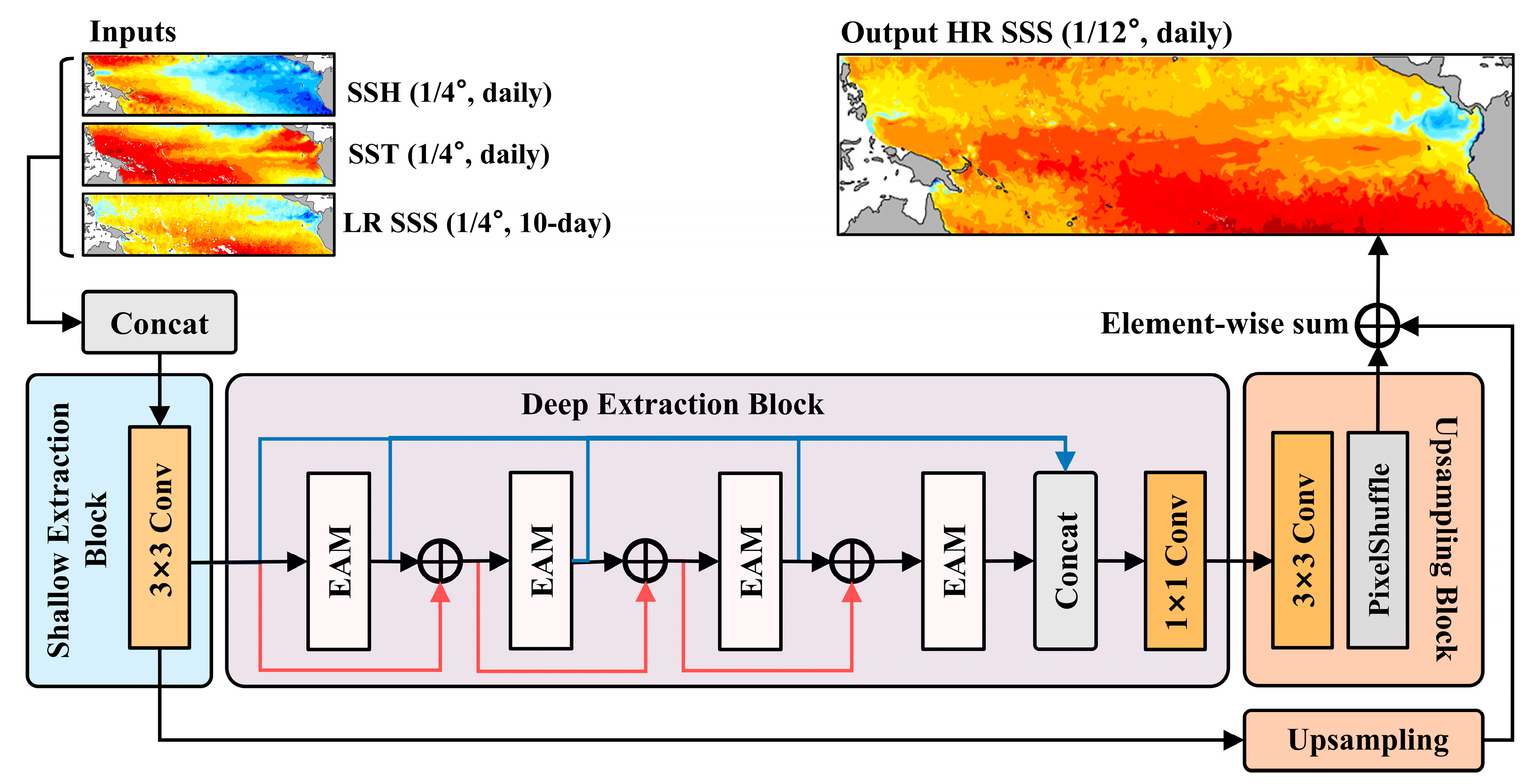
There have been many Transformer-based SR models widely used in the field of computer vision, but they have hardly been applied to SR reconstruction of satellite SSSs up until the present. Therefore, the TSR model is proposed here, which integrates three grid files of NRT satellite sea surface observation data to realize SR reconstruction from a 1/4° and 10-day mean to a 1/12° and daily mean resolution. As shown in Figure 2, TSR requires two training stages to sequentially learn the label information from the reanalysis gridded fields and the in situ scattered observations.

3.1. TSR

3.1.1. Overall Architecture of TSR

As shown in Figure 2, our TSR consists of three parts: shallow extraction block, deep extraction block, and upsampling block. The SR task can be expressed as follows:

$$Y={\mathcal{F}}_{TSR}\left(V,\theta \right)$$

(1)

$$V=concat\left[V_{LR SSS},V_{SST}, V_{SSH}\right]$$

(2)

where ${\mathcal{F}}_{TSR}(·)$ represents our model TSR; $\theta$ denotes the model parameters; $Y$ is the SR result of TSR; and $V$ is the LR input tensor $I_{LR}\in {\mathbb{R}}^{3\times H\times W}$ of all input variables concatenated together by $concat(·)$ in the channel dimension, with three channels corresponding to three variables, SSS from SMOS, SST from RSS, and SSH from CMEMS, where $H$ and $W$ represent the height and width of the input tensor.

First, given the input tensor, $I_{LR}$, to extract potential SR features of multivariate information in advance, we employ a $3\times 3$ convolutional layer from the shallow extraction block to generate the shallow feature $F_S\in {\mathbb{R}}^{C\times H\times W}$:

$$F_S=f_S\left(I_{LR}\right)$$

(3)

where $C$ is the number of channels, and $f_S$ denotes the shallow extraction block.

Subsequently, the shallow feature, $F_S$, undergoes the deep extraction block (see Section 3.1.2 for details) to acquire the deep feature, $F_D\in {\mathbb{R}}^{C\times H\times W}$. This stage consists of multiple enhanced attention modules (EAMs; see Section 3.1.3 for details) connected by using residuals and dense connections. The deep extraction block can be expressed as follows:

$$F_D=f_D\left(F_S\right)$$

(4)

where $f_D$ denotes the deep extraction.

Finally, we upsample $F_D$ and $F_S$ separately using the upsampling block that includes a $3\times 3$ convolutional layer and a PixelShuffle layer. Next, they are skip-connected using element-wise sum to obtain the high-resolution output, HR SSS $O_{HR}\in {\mathbb{R}}^{1\times H\times W}$:

$$O_{HR}=f_p\left(f_c\left(F_S\right)\right)+f_p\left(f_c\left(F_D\right)\right)$$

(5)

where $f_c$ and $f_p$ denote the convolutional and PixelShuffle layer, respectively.

3.1.2. Deep Extraction Block

In the ocean, there are complex long- and short-range dependencies, and these local ocean processes with distance but similar spatial structures can be used as references to each other to restore the spatial details. Compared to CNN, which is limited to the local operation of convolution, Transformer can capture global dependencies based on self-attention [40] and therefore can exploit richer reference information to improve the accuracy of SR.

In this paper, deep extraction employs residual and dense connections to combine self-attention-based EAMs for capturing the global dependencies. Residual connections alleviate training complexities and improve convergence speed by flowing feature information across layers, making it easier to keep learning valid features even when the network has deeper layers. Dense connections aggregate multiscale feature information from each EAM, thus further improving the expressiveness of the network and reducing information loss. Residual connectivition is used between each EAM module, and dense connectivity is used at the end of all EAMs, with multiscale features fused by a $1\times 1$ convolutional layer, compressed to the original number of channels. The expressions of deep extraction are as follows:

$$F_D^l=\left\{\begin{array}{c}{f}_E^1\left(F_S\right)+F_S, l=1\\ f_E^l\left(F_D^{l-2}+F_D^{l-1}\right), l\ge 2\end{array}\right.$$

(6)

$$F_D=f_D\left(F_S\right)=f_c\left(concat\left[F_D^1,F_D^2,\dots ,F_D^l\right]\right), l\in \left.\left\{1, 2,\dots ,L\right.\right\}$$

(7)

where $F_D^l\in {\mathbb{R}}^{C\times H\times W}$ is the deep feature after the l-th EAM, $l\in \left.\left\{1, 2,\dots ,L\right.\right\}$, and $f_E^l$ denotes the EAM.

3.1.3. EAM

Instead of following the mainstream “Norm → Attention → Norm → MLP” flow of the standard transformer’s encoder, EAM replaces MLP with a convolutional layer for further restoring the neighborhood similarity of Attention that has extracted global dependencies [41].

As shown in Figure 3a, EAM consists of two successive stages, which are the Multi-Head Attention (MHA) and the convolutional layer. Before these two stages, unfolding and folding operations [42] are performed to adapt the dimensions of the input tensor to the MHA and the convolutional layer, respectively. In addition, layer normalization is performed before both the MHA and the convolutional layer, and the residual connection is performed after both. Assuming that the input tensor of the EAM is $F$, the expressions for these two stages are as follows:

$$F_{MHA}=MHA\left(Norm\left(f_{unfold}\left(F\right)\right)\right)+f_{unfold}\left(F\right)$$

(8)

$$F_D^l=f_c\left(Norm\left(f_{fold}\left(F_{MHA}\right)\right)\right)+f_{fold}\left(F_{MHA}\right)$$

(9)

where $f_{unfold}$ is the unfolding operation; $f_{fold}$ is the folding operation; and $MHA(·)$ and $Norm(·)$ represent the MHA and layer norm operations, respectively.

Following the standard transformer [40], the MHA is shown in Figure 3b. MHA consists of multiple independent heads that compute global attention separately and are finally concatenated. The global attention is calculated by scaled dot-product attention (SDPA):

$$SDPA(Q_h,K_h,V_h)=softmax\left({\displaystyle \frac{Q_h{K}_h^T}{\sqrt{L}}}\right)V_h$$

(10)

where $Q_h,K_h$, and $V_h$ represent the tensor obtained by mapping the input through linear layers at the h-th head, $h\in \left.\left\{1, 2,\dots ,H\right.\right\}$; and $L$ is the dimension of $Q_h,K_h$, and $V_h$.

3.2. Progressive Transfer Learning Strategy for TSR

In this paper, two types of data, both the reanalysis gridded field and the in situ scattered observations, are adopted as the label. The high-resolution reanalysis gridded field provides the reference for the complete and continuous spatial structure of the ocean processes at multiple scales for SR. However, the ocean reanalysis products may have systematic or random deviations from the actual salinity in some regions [36,43]. Compared with reanalysis gridded field, although in situ measurements are more accurate, their distribution is very sparse and uneven in both space and time [44], implying that scattered observations are fewer and their locations are not fixed on every single day, and thus it has no complete spatial structure and cannot provide reference values for all grids. Therefore, it is necessary to combine the advantages of gridded fields and scattered in situ observations to provide higher-quality labels for SR.

Transfer learning is capable of inheriting prior knowledge and quickly adapting to new tasks [45], which is suitable for knowledge transfer between different tasks. Transfer learning assumes that there is shared knowledge or features (such as underlying visual features or model structures) between different tasks [46,47]. This shared knowledge can be transferred from the original task to the new task, thereby avoiding the need to learn the new task from scratch [48]. Typically, transfer learning involves first training on a large dataset (source domain) [49] to learn general knowledge. The trained model is then applied to a new small dataset (target domain) [49] for further training. This enables rapid fine-tuning of the model’s parameters to make it adaptable to the new task [49].

For the gridded labels from reanalysis products and the scattered labels from in situ observations, they have shared SSS knowledge, which meets the premise of transfer learning. Meanwhile, they can be regarded as two tasks. The gridded labels from reanalysis products are the source domain with a large number of samples, and the sparse, scattered labels from in situ observations can be regarded as the target domain with a small number of samples. Therefore, TSR can first learn the knowledge of the general spatiotemporal distribution of SSS under the guidance of gridded labels, especially the knowledge of complete and continuous spatial features that cannot be provided by sparse scatter points. Then, because reanalysis products are driven by ocean dynamic models, their results for some locations may not be as accurate as in situ observations [50]. Therefore, by training with new scattered labels from in situ observations, parameters of TSR would be further fine-tuned. Finally, the output of TSR can be further corrected to more closely match in situ observations.

However, there are huge differences in the spatial and temporal distribution of the two label types. Directly switching label types in general transfer learning may cause conflicts, resulting in the inability to further improve model performance in new tasks. Therefore, to alleviate the training difficulties caused by the significant differences in time and space between gridded and scattered labels, we followed the idea of curriculum learning [51]. This makes the training difficulty gradually increase from easy to difficult, ensuring that the training model gradually converges.

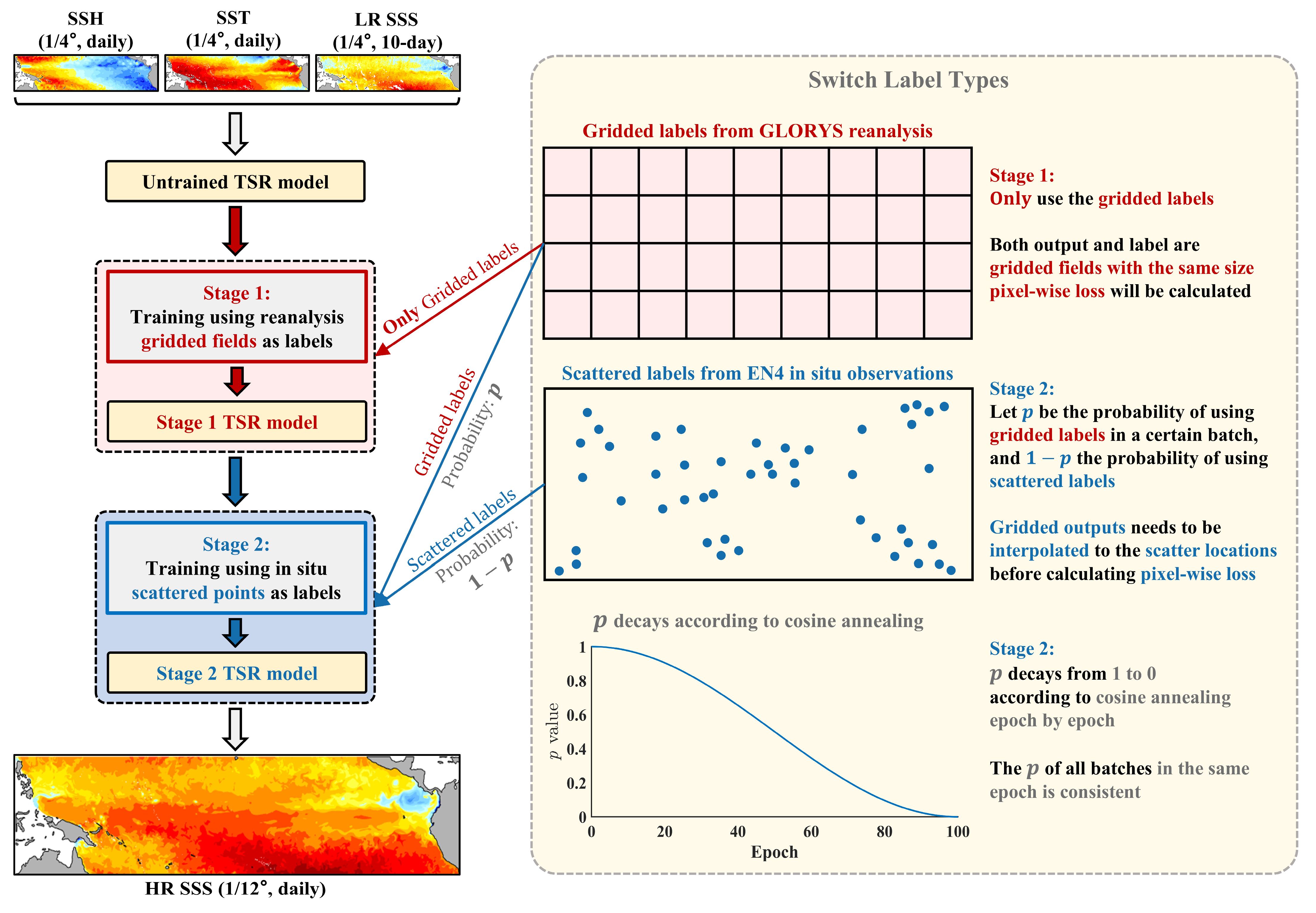
As shown in Figure 4, the left side shows the overview of the TSR training process, which consists of two stages. The right side of Figure 4 shows the specific steps for switching training labels, detailing how the two types of labels are used in each stage. In Stage 1, the TSR is trained with the gridded labels from the reanalysis product GLORYS to learn the complete and continuous spatial distribution of oceanic dynamical processes. In Stage 2, the Stage 1 TSR model used to complete the Stage 1 training will continue to be trained using scattered labels from in situ observations. Stage 2 uses scattered in situ data as labels to further correct errors in the grids covered by scattered points in the output gridded SR results. Note that the outputs of the TSR models for both Stage 1 and Stage 2 are two-dimensional (2D) gridded fields.

Since both the Stage 1 outputs and labels are 2D gridded fields of the same size, the pixel-wise loss can be calculated directly. The gridded outputs from Stage 2 are first interpolated to the spatial locations of the scattered points, and then the pixel-wise loss is calculated (see Section 3.3 for details).

In order to achieve a smooth transfer between the two label types, we progressively replace the gridded labels with the scattered labels, rather than replacing them all at once. Specifically, the cosine annealing strategy is used to decay the probability of using gridded labels from 1 to 0 epoch by epoch. Suppose that the probability of using gridded labels in a certain epoch is $p$. Then, each training batch in that epoch has a probability, $p$, to use the gridded labels. Since only one type of label can be used in the same training batch, the probability of using scattered labels is $(1-p)$.

As the epoch increases, $p$ smoothly decreases from 1 to 0 according to cosine annealing. This means that the probability of using scattered labels will progressively increase, while the probability of using gridded labels will progressively decrease. The expression for the cosine annealing of $p$ is as follows:

$$p_e=p_{min}+{\displaystyle \frac{1}{2}}\left(p_{max}-p_{min}\right)\left(1+cos\left({\displaystyle \frac{e}{E}}\pi \right)\right)$$

(11)

where $p_e$ is the percentage of gridded fields at the e-th epoch; $e\in \left.\left\{1, 2,\dots ,E\right.\right\}$; $E$ is the total number of decaying epochs; and $p_{max}$ and $p_{min}$ are the maximum and minimum bounds of $p$, i.e., 1 and 0, respectively.

Compared with replacing all labels at once, the PTL strategy helps the TSR model fully adapt to the new label type and therefore increases the SR accuracy. Otherwise, it may lead to overfitting: the TSR model that has been adapted to a certain label type can no longer adapt to the new label type, resulting in a decrease in accuracy.

3.3. Implementation Details

For gridded labels, a pixel-wise L1 loss is used. For scattered labels, the grid-based SR results are first interpolated to the spatial locations of each scattered point using bilinear interpolation, and then the L1 loss is calculated:

$$L_{grid}={\displaystyle \frac{1}{N_{grid}}}{\sum }_n^{N_{grid}}\left|\left(X_n^{grid}-Y_n^{grid}\right)\right|$$

(12)

$$L_{insitu}={\displaystyle \frac{1}{N_{insitu}}}{\sum }_n^{N_{insitu}}\left|\left(X_n^{insitu}-Y_n^{insitu}\right)\right|$$

(13)

where $L_{grid}$ and $L_{insitu}$ are the gridded and scattered losses, respectively; $N_{grid}$ represents the number of grids in ocean areas; $N_{insitu}$ represents the number of in situ scattered observations available; $X_n^{grid}$ and $Y_n^{grid}$ denote the n-th grid at the same location in the gridded output and gridded labels, respectively; and $X_n^{insitu}$ and $Y_n^{insitu}$ denote the n-th scatter at the same position in the interpolated output and scattered labels, respectively.

TSR is implemented using the PyTorch [52] framework, using the AdamW [53] optimizer with parameters $\beta 1=0.9$ and $\beta 2=0.99$, with a learning rate of 0.001, and batch size set to 4. All random seeds are fixed to 32 to ensure consistent initialization. To train adequately, we set a patience parameter. If the error on the validation set did not decrease by at least 0.0001 within 20 epochs, the training was halted.

In addition, in TSR, we set all convolutional layers followed by PReLU activation and batch normalization, except for the last convolutional layer. The number of feature channels in all hidden layers is 32. There are 8 EAMs in the deep extraction block. The number of heads in MHA is set to 4. Meanwhile, the convolution kernel size in EAM is 9 × 9. The process of finding the optimal hyperparameter settings is detailed in Section 5.1 (“Ablation Experiments”).

4. Results

4.1. Experimental Setup

In this section, TSR is compared with mainstream satellite SSS products (SMOS and SMAP), we analyze their spatial and temporal accuracy, and we demonstrate its ability to capture mesoscale processes. We employed four evaluation metrics: the mean absolute error (MAE), root mean square error (RMSE), mean bias (MB), and coefficient of determination R². A smaller MAE and RMSE indicate lower errors, while an MB value closer to 0 indicates a smaller bias. A higher R² value is better.

$$MAE={\displaystyle \frac{{\sum }_n^N\left|X_n-Y_n\right|}{N}}$$

(14)

$$RMSE=\sqrt{{\displaystyle \frac{1}{N}}{\sum }_n^N{{(X}_n-Y_n)}^2}$$

(15)

$$MB={\displaystyle \frac{{\sum }_n^N{(X}_n-Y_n)}{N}}$$

(16)

$$R^2=1-{\displaystyle \frac{{\sum }_n^N{\left(X_n-Y_n\right)}^2}{{\sum }_n^N{\left(Y_n-\overline{Y}\right)}^2}}$$

(17)

where $Y_n$ denotes the observation at a certain location in the validation data, and $X_n$ denotes the result of interpolating the gridded output of TSR to the corresponding location. There is a total of $N$ validation data points.

4.2. Spatial Analysis

The detailed results of TSR and other SSS products compared to EN4 are presented in

Table 2. Performance metrics of TSR and other SSS products compared to EN4 in the test set (2022 and 2023). The best and second-best results are in bold and italics, respectively.

Model	MAE (psu)	RMSE (psu)	MB (psu)	${\mathit{R}}^{\mathbf{2}}$
TSR	0.1226	0.1647	−0.0075	0.9482
GLORYS	0.1004	0.1615	−0.0344	0.9502
SMOS	0.1884	0.2457	−0.0394	0.8848
SMAP	0.1609	0.2198	−0.0955	0.9078

. Overall, TSR’s performance is second only to GLORYS in all metrics, but it is the best in MB. Compared to the input SMOS product, TSR reduces MAE by about 38% (from 0.1884 psu to 0.1226 psu), RMSE by about 33% (from 0.2457 psu to 0.1647 psu), and MB by about 81% (from −0.0394 psu to −0.0075 psu), and it improves R² by about 7% (from 0.8848 to 0.9482). The significant improvement in MB of TSR may be attributed to the PTL enabling the TSR to further correct the bias, as analyzed in detail in Section 5.2 (“Comparison of Decay Schemes and Training Strategies”).

As shown in Figure 5, the TSR has a smaller overall error, and its pattern is closer to that of the in situ SSS. Compared to SMAP, the TSR has a smaller error on the east coast of the equatorial Pacific. Meanwhile, TSR significantly reduces the error in the global range of SMOS. Compared to GLROYS, TSR has smaller errors in the central and eastern equatorial Pacific region (170°E–165°W, 3°N–3°S) and (160°W–125°W, 0°–10°N), which implies that TSR can more accurately capture large-scale climate changes in the equatorial Pacific, such as El Niño and La Niña events.

Given the regional and event-specific variability present in the study area, but no obvious seasonal differences around the equator, we will present the analysis of typical subregions month by month. In the test set, we evaluated the monthly accuracy of TSR and other SSS products under four ranges compared to EN4. The four ranges are (a) the entire study area of the equatorial Pacific region (130°E–70°W, 20°S–20 N); (b) the coverage area of ENSO indices, namely the Niño 1 + 2, 3.4, and 4 region (160°E–90°W, 5°S–5°N) and (90°W–80°W, 10°S–0°); (c) the eddy-concentrated eastern equatorial Pacific region within the study area (120°W–75°W, 5°S–15°N); and (d) the western boundary current region within the study area (120°E–170°E, 20°S–20°N). Due to an extended downtime period for the SMAP from August 6 to September 23, 2022, the evaluations do not include August and September 2022.

Overall, as shown in Figure 6a, across the entire study area, although TSR performs slightly worse than GLORYS in terms of MAE, it is comparable to GLORYS in terms of RMSE and $R^2$, with no significant difference. In particular, MB of TSR is closer to 0 psu, while GLORYS is generally lower, indicating that the error correction based on in situ data by PTL effectively offsets the systematic underestimation caused by GLORYS as a labels In contrast, SMOS and SMAP performed poorly in all performance indicators, further demonstrating that TSR effectively improved the accuracy of the input SMOS and maintained a stable level of improvement in all months. Region (b) is the coverage area for the primary Niño indices used to assess El Niño events. TSR’s RMSE and MAE are comparable to GLORYS overall, with $R^2$ of TSR performing the best, indicating that reconstruction results of TSR can more accurately capture the dynamics of El Niño events. However, on the MB, the trends of TSR and SMOS are highly consistent, leading to relatively higher bias in TSR from October 2022 to February 2023. This suggests that the error correction by PTL is still insufficient in the equatorial region. In region (c), TSR is comparable to GLORYS in terms of MAE, RMSE, and $R^2$, and it significantly outperforms SMOS. On the MB, TSR performs the best. This suggests that in regions with dense mesoscale eddies, the SR reconstruction results from TSR are likely to identify eddy dynamics. This will be further analyzed below. In region (d), TSR and GLORYS are closely matched in all metrics, indicating that TSR also achieves ideal SR reconstruction accuracy in large-scale ocean current regions.

In summary, TSR maintains a stable performance across different months and typical subregions, demonstrating its potential for adaptation to various application scenarios (such as large-scale climate anomalies and mesoscale eddy identification).

To further analyze the reconstruction performance of TSR for oceanic multiscale processes, we compare the SSS and SSS anomalies (SSSAs) for the global and eddy-concentrated eastern equatorial Pacific region, as shown in Figure 7 and Figure 8, respectively.

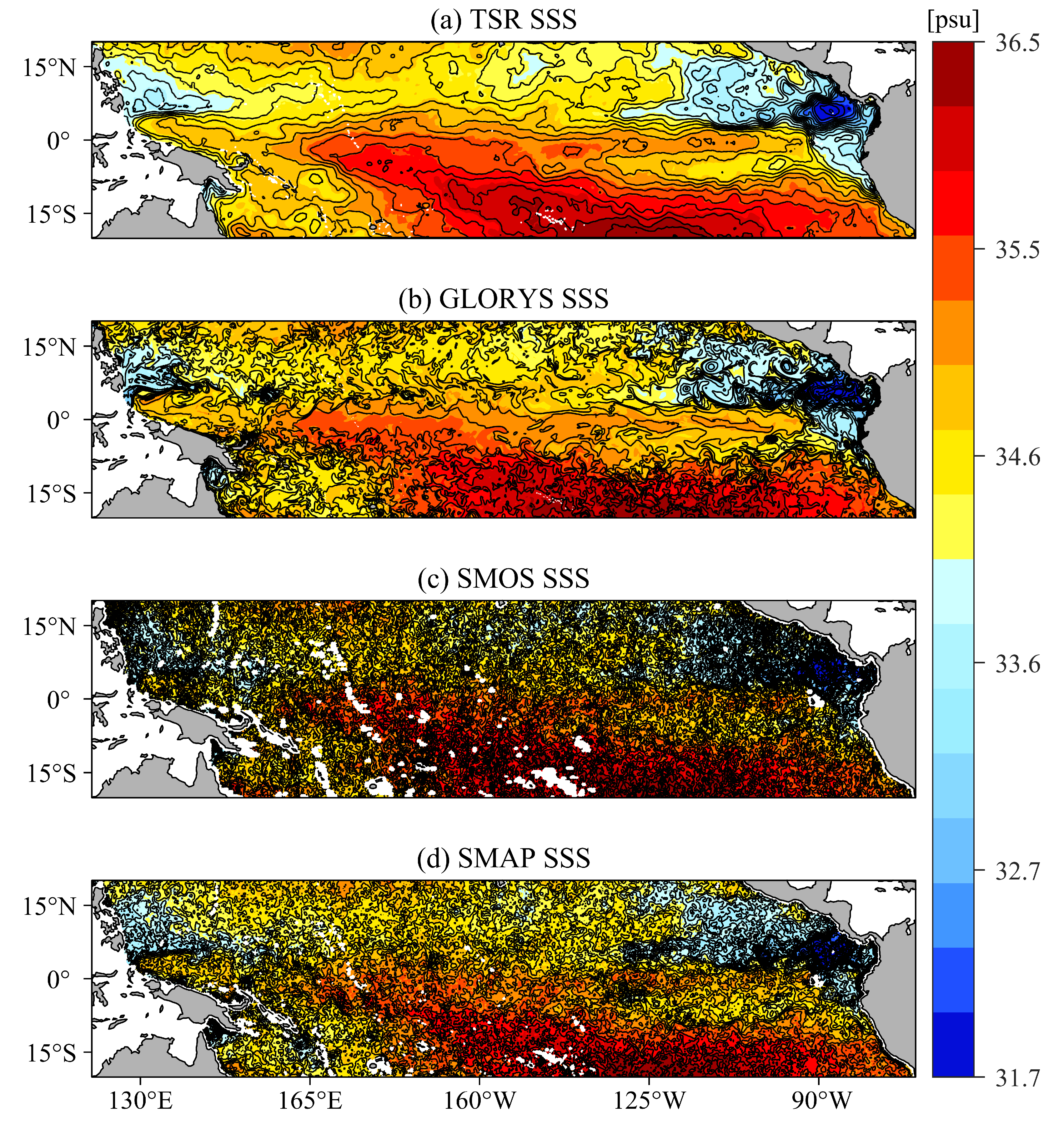
Figure 7 enables a clearer observation of the structure of eddies and fronts in the SSS, as well as the distribution of noise, by overlaying the contours. As shown in Figure 7c,d, the cluttered contours in SMOS and SMAP are spread throughout the image, indicating that they are both covered by a large amount of noise, and thus it is almost impossible to resolve any organized systems, such as fronts, eddies, etc., from them. The contours of TSR and GLORYS are clearer, and in the eastern equatorial Pacific, several closed contours can be observed, indicating the existence of eddies. Overall, TSR effectively reduces the noise of SMOS and enhances the eddy structures.

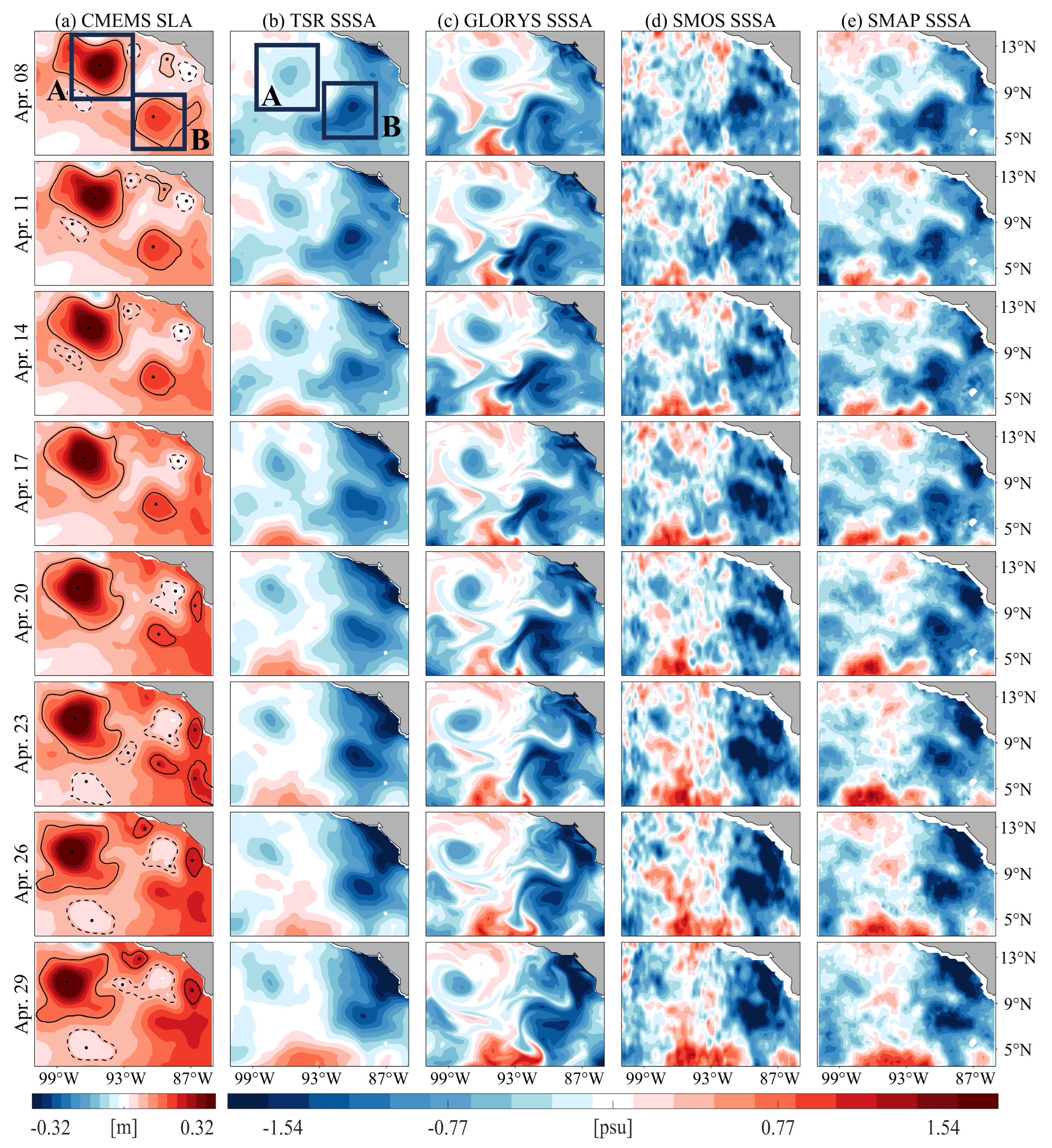
Figure 8 illustrates the process of eddy dynamics in the eddy-dense region of the eastern equatorial Pacific. In Figure 8, the cyclonic eddies (dashed lines) and anticyclonic eddies (solid lines) identified by the SSH-based method are overlaid in the CMEMS SLA. Since salinity is not fully considered a passive tracer, the spatial extent and degree of anomalies in the SSS may not be fully synchronized with changes in the SLA. However, typical variations corresponding to the SLA, such as mesoscale eddies, can still be observed in the SSSA.

In the CMEMS SLA (Figure 8a), we select two typical anticyclonic vortices, Eddy A and Eddy B. Over time, the structure of Eddy A remains stable, with a slight tendency to move westward, whereas Eddy B progressively shrinks while merging with the eddies along the shoreline, and ultimately disappears. As shown in Figure 8b, TSR can resolve SSSA eddies corresponding to Eddy A and Eddy B. Eddy A produced the same westward trend over time, while Eddy B gradually moved closer to the anomaly signal along the coast and eventually merged and disappeared. However, it is almost impossible to distinguish clear eddy structures in SMOS SSSA, and there are quite a few white-noise spots. Although the eddy structure of the SMAP SSSA on April 8 was relatively clear, it became increasingly fuzzy with time and was difficult to identify accurately in the interference of the surrounding anomaly signals.

4.3. Temporal Analysis

Taking the long-time series of in situ observations provided by the moored buoys TAO on the equatorial Pacific as references, we analyze the performance of TSR in terms of improved temporal resolution compared to other SSS products.

We first analyze the accuracy of the complete time series of each buoy. As shown in

Table 3. Performance metrics of TSR and other SSS products compared to TAO in the test set (2022 and 2023). The best and second-best results are in bold and italics, respectively.

Model	MAE (psu)	RMSE (psu)	MB (psu)	${\mathit{R}}^{\mathbf{2}}$
TSR	0.1229	0.1625	−0.0101	0.9152
GLORYS	0.1170	0.1801	−0.0470	0.8959
SMOS	0.1931	0.2434	−0.0273	0.8099
SMAP	0.1601	0.2096	−0.1047	0.8590

, except for MAE, which is slightly higher than GLORYST, TSR achieves optimal performance in all metrics, compared to other products. This may be due to the denser distribution of EN4 near the equator (Figure 1), enabling the SR results in this region to be more fully corrected. Therefore, the accuracy improvement of TSR is more significant in the TAO-covered region, i.e., along and near the equator, compared to the whole study area.

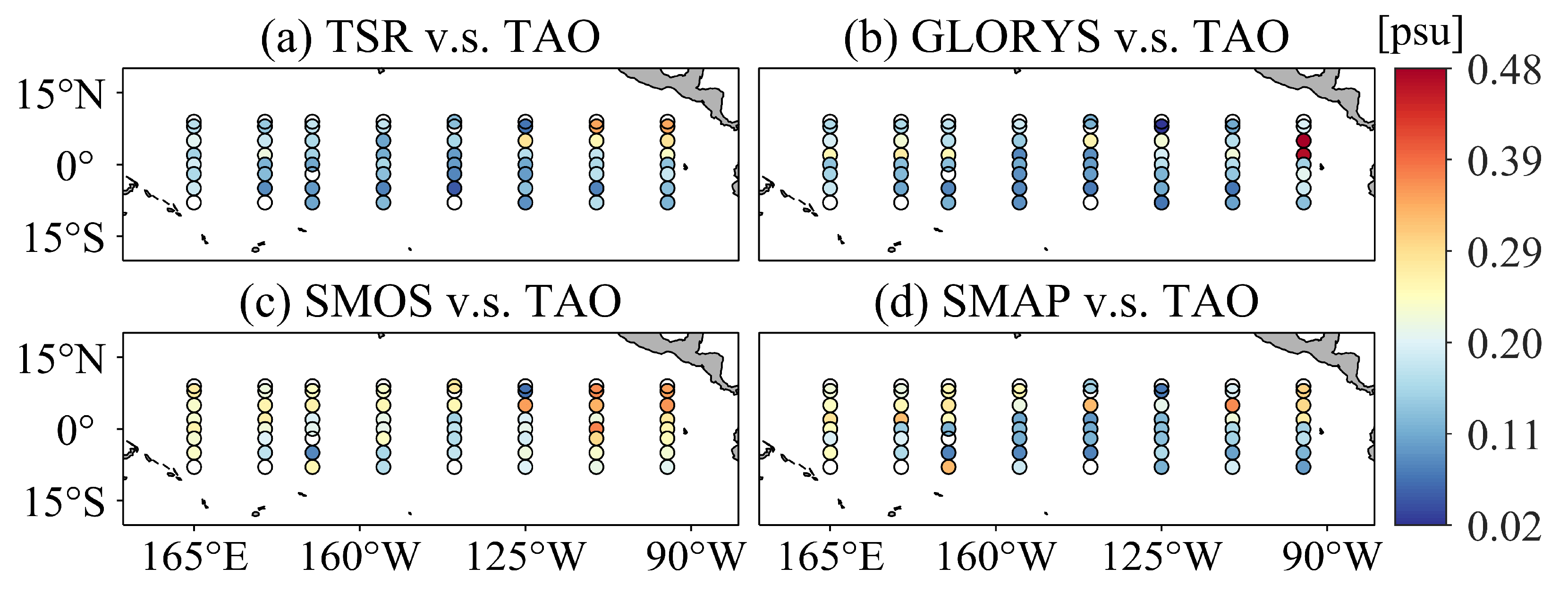
As shown in Figure 9, the RMSE for TSR is generally lower than that for SMOS and SMAP. Although the TSR is slightly higher than the GLORYS error on buoys along 110°W, it is significantly lower along 95°W.

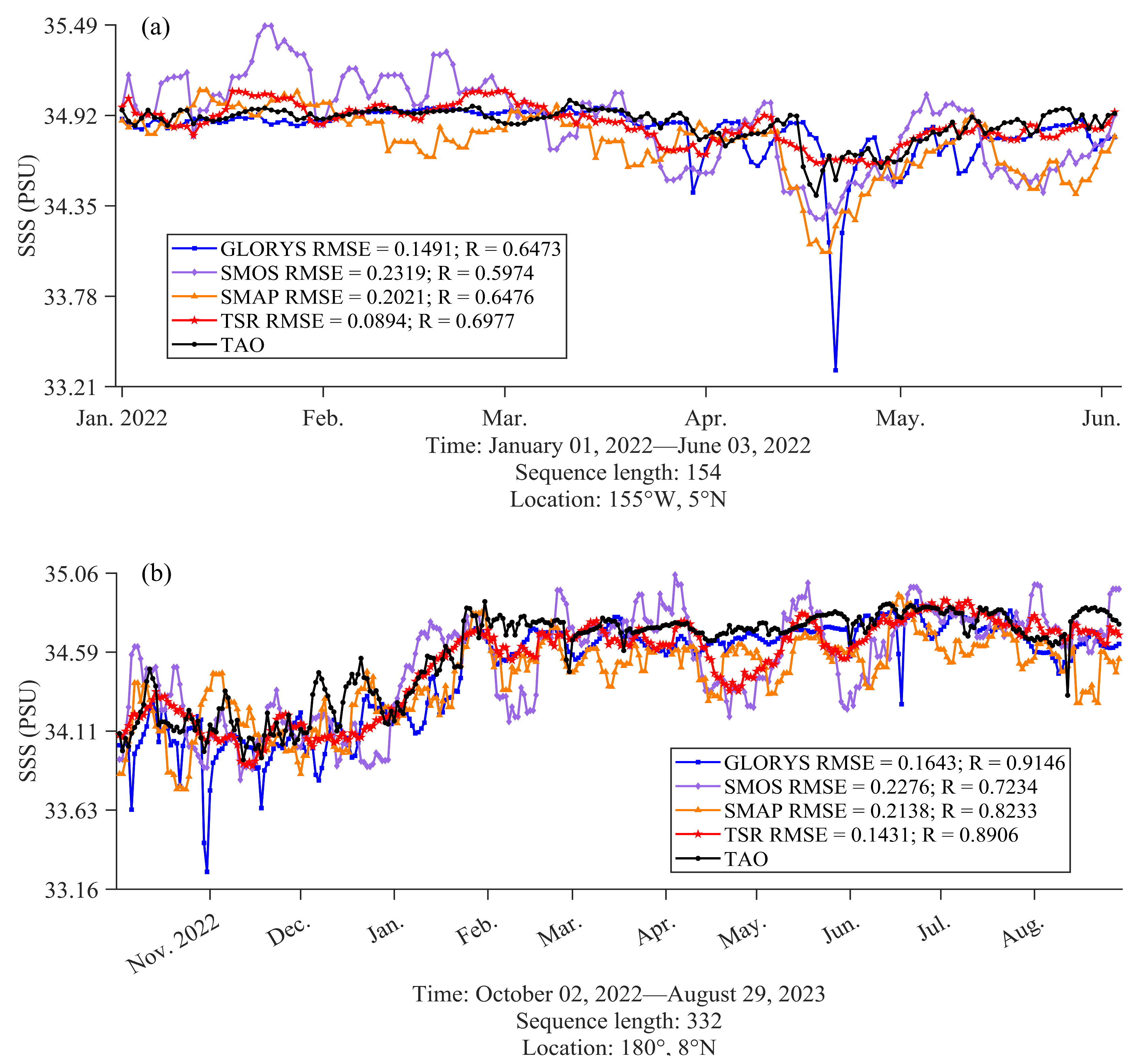
For temporal analysis, we selected two typical buoys with continuous long-term series at (155°W, 5°N) and (95°W, 5°S), respectively (Figure 10), due to possible interruptions in the data provided by TAO. As shown in Figure 10a, at the site (155°W, 5°N), the time series of TSR and TAO generally match, and the RMSE and correlation coefficient (R) of TSR are significantly better than those of other products. However, the time series of SMOS and SMAP remains unreasonably overestimated or underestimated overall. Before April 2022, the time series of GLORYS and TAO match, but after April 2022, there are obvious fluctuations and even sharp spikes. At site (95°W, 5°S) (Figure 10b), although there is some underestimation of the TSR time series from April to June 2023, the overall trend remains stable and, therefore, only slightly below GLORYS in R, while RMSE is optimal. In contrast, there are significant ups and downs in the series of SMOS, and the series of SMAP remains lower than TAO after April 2023.

Overall, the time series of TSR is basically the same as that of TAO, which is a significant improvement compared to SMOS, indicating that TSR can effectively improve the temporal resolution of SMOS to about a daily scale.

5. Discussion

5.1. Ablation Experiments

To achieve better SR results, the main hyperparameters of TSR also need to be appropriately set. There are five main structural hyperparameters: the number of EAMs, the number of feature channels in hidden layers, the number of MHA heads, and the size of the convolutional kernel in EAMs. The results are shown in

Table 4. Performance metrics for different EAM numbers compared to EN4 in the test set. The best and second-best results are in bold and italics, respectively.

EAM Number	MAE (psu)	RMSE (psu)	MB (psu)	${\mathit{R}}^{\mathbf{2}}$
2	0.1321	0.1771	−0.0344	0.9401
4	0.1302	0.1747	−0.0358	0.9418
6	0.1305	0.1747	−0.0355	0.9418
8	0.1296	0.1736	−0.0339	0.9425
10	0.1309	0.1746	−0.0397	0.9418

,

Table 5. Same as Table 4, but for the hidden layers’ channel number.

Hidden Layers’ Feature Channel Number	MAE (psu)	RMSE (psu)	MB (psu)	${\mathit{R}}^{\mathbf{2}}$
4	0.1367	0.1820	−0.0374	0.9368
8	0.1348	0.1796	−0.0368	0.9385
16	0.1296	0.1736	−0.0339	0.9425
32	0.1281	0.1718	−0.0353	0.9437
64	0.1313	0.1752	−0.0388	0.9414

,

Table 6. Same as Table 4, but for the MHA head number.

MHA Head Number	MAE (psu)	RMSE (psu)	MB (psu)	${\mathit{R}}^{\mathbf{2}}$
1	0.1299	0.1734	−0.0359	0.9426
2	0.1297	0.1732	−0.0371	0.9427
4	0.1281	0.1718	−0.0353	0.9437
8	0.1291	0.1723	−0.0350	0.9433
16	0.1335	0.1772	−0.0505	0.9401

,

Table 7. Same as Table 4, but for the convolutional kernel size in EAM.

Convolutional Kernel Size in EAM	MAE (psu)	RMSE (psu)	MB (psu)	${\mathit{R}}^{\mathbf{2}}$
1	0.1349	0.1785	−0.0529	0.9392
3	0.1281	0.1718	−0.0353	0.9437
5	0.1280	0.1716	−0.0346	0.9438
7	0.1280	0.1707	−0.0374	0.9444
9	0.1262	0.1695	−0.0277	0.9452
11	0.1286	0.1722	−0.0353	0.9434
13	0.1290	0.1727	−0.0325	0.9431
15	0.1286	0.1716	−0.0371	0.9438
17	0.1354	0.1803	−0.0498	0.9380

and

Table 8. Same as Table 4, but for learning rate.

Learning Rate	MAE (psu)	RMSE (psu)	MB (psu)	${\mathit{R}}^{\mathbf{2}}$
0.1	0.1617	0.2123	−0.0652	0.9140
0.01	0.1559	0.2053	−0.0643	0.9196
0.001	0.1262	0.1695	−0.0277	0.9452
0.0001	0.1286	0.1718	−0.0314	0.9436
0.00001	0.1398	0.1856	−0.0528	0.9342

. Note that when the convolution kernel size is $1\times 1$, it is equivalent to an MLP. Therefore, the experimental results in Table 7 also include the results of ablation experiments where the MLP in the Transformer encoder was replaced with a convolutional layer.

As the number of EAMs and the number of channels in hidden layers increase, the SR accuracy improves because the model has stronger feature extraction capabilities. However, overly deep networks carry the risk of overfitting, which can lead to a decline in performance. Similarly, increasing the number of heads in MHA and the size of the convolution kernel in EAMs facilitates the learning of richer long-range and short-range dependencies, but the learning effect begins to decline after oversaturation. On the other hand, the learning rate is an important factor affecting the model’s training performance and generalization capabilities. As shown in Table 8, setting the learning rate to 0.001 achieves a higher SR accuracy.

Therefore, as shown in the results of Table 4, Table 5, Table 6, Table 7 and Table 8, we selected the hyperparameter settings that achieved the best performance for TSR. We set the number of EAMs to 8, the number of channels in hidden layers to 32, the number of heads in MHA to 4, the size of the convolutional kernel in EAMs to 9, and the learning rate to 0.001.

5.2. Comparison of Decay Schemes and Training Strategies

In this section, we evaluate the impact of different decay schemes and training strategies on model performance. The results are shown in

Table 9. Performance metrics for different decay schemes in PTL compared to EN4 in the test set. The best and second-best results are in bold and italics, respectively.

Decay Scheme	MAE (psu)	RMSE (psu)	MB (psu)	${\mathit{R}}^{\mathbf{2}}$
Cosine Annealing	0.1226	0.1647	−0.0075	0.9482
Stepped	0.1235	0.1654	−0.0074	0.9478
Linear	0.1232	0.1652	−0.0113	0.9479
Exponential	0.1230	0.1649	−0.0088	0.9481

and

Table 10. Performance metrics of TSR and other training strategies compared to EN4 in the test set (2022 and 2023). The best and second-best results are in bold and italics, respectively.

Model	Configuration	MAE (psu)	RMSE (psu)	MB (psu)	${\mathit{R}}^{\mathbf{2}}$
TSR	PTL strategy	0.1226	0.1647	−0.0075	0.9482
TSR1	One-step training and only using gridded labels	0.1262	0.1695	−0.0277	0.9452
TSR2	One-step training and only using scatter labels	0.3616	0.4783	−0.0711	0.5634
TSR3	One-step training and using both gridded and scatter labels	0.1514	0.2007	−0.0346	0.9231
TSR4	Two-step training, but not progressive, using gridded and scatter labels successively	0.3649	0.4939	−0.0935	0.5346

.

We compare four main schemes for decaying the probability of using gridded labels in PTL: cosine annealing, stepped decay, linear decay, and exponential decay. Stepped decay refers to the probability, $p$, of using grid labels decreasing from 1 to 0 once every 10 epochs, with a total of 10 steps. Linear and exponential decay refer to the probability, $p$, decreasing from 1 to 0 according to a linear or exponential trend per epoch.

As shown in Table 9, the cosine annealing scheme improves the performance of TSR most significantly. Although it is slightly worse than the stepped decay scheme in MB, the cosine annealing scheme still has a significant advantage in terms of the performance of the other three indicators.

After setting the decay scheme in PTL to cosine annealing, we compared the performance of the model under different training strategies. TSR1 denotes one-step training and only using grid labels; TSR2 denotes one-step training and only using scattered labels; TSR3 denotes one-step training using both gridded and scattered labels, i.e., summing up the $L_{grid}$ and $L_{insitu}$ as the total loss; and TSR4 denotes two-step training with first using grid labels and then scattered labels, meaning that the model trained in TSR1 continues to be trained using scattered labels, but there is no progressive transition between two stages based on cosine annealing.

As shown in Table 10, the TSR obtained by training with the PTL strategy achieves the globally optimal performance, especially on the MB. The performances of the remaining four strategies are TSR1, TSR3, TSR2, and TSR4 in that order. First, TSR1 (one-step training and only using scatter labels) is used as a benchmark to compare TSR2 (one-step training and using only scatter labels) and TSR3 (one-step training and using both gridded and scatter labels). The results show that when a large number of in situ observation scatter labels are directly introduced, there is a significant decline in model performance regardless of whether or not gridded labels continue to be used, i.e., TSR2 and TSR3. Therefore, the direct introduction of more in situ data fails to correct the error. Second, if more in situ data are introduced but transfer learning without an annealing scheme, i.e., TSR4 (two-step training but not progressive, using gridded and scatter labels successively), the performance of the model is also significantly degraded. Therefore, in order to improve the accuracy, especially to reduce the bias, the introduction of in situ data and the use of the annealing scheme for transfer learning in the PTL strategy are indispensable.

In fact, each grid has an independent time series, and each time series corresponds to the statistical distribution of all historical SSS values for that grid position. Meanwhile, the TSR model is a field-to-field model: the inputs, labels, and outputs are all 2D fields. When training with gridded labels, it is able to provide historical experience for each grid of the TSR to learn. Subsequently, the TSR reconstructs all grids simultaneously, forming the entire output gridded fields. However, when using in situ observation scatters as labels, only a small number of grids are able to be guided by the scatter labels during training. This is because the number and spatial location of scatters for each day are very sparse and random. In other words, when using scatter labels, the optimization direction of model training is not for the entire file but rather for certain grids covered by scatter labels. Therefore, that inappropriate optimization direction may have led to the overall accuracy degradation. Furthermore, when the model is trained with both gridded and scatter labels, i.e., TSR3, it actually changes the statistical distribution of each grid provided when only gridded labels are used, leading instead to a decrease in SR accuracy.

In summary, these experiments indicate that directly replacing the training label types for transfer learning does not yield the desired results, but rather leads to a decrease in model performance. The PTL strategy ensures that TSR can be sequentially trained on gridded and scatter labels to improve SR accuracy. In addition, the gradual transition based on the annealing strategy provides a reliable reference for transfer learning when switching between different training label types.

5.3. Comparison of Input Variables

To compare the performance differences between different combinations of input variables, we trained five models labeled with grid fields. The reasons for choosing SST and SSH as auxiliary input variables are as follows. On the one hand, SSS, SST, and SSH show similar structures of variation in the same oceanic process, so they can provide more reference information for SR. On the other hand, the existing satellite observations of SST and SSH are of better quality, as well as higher spatial and temporal resolution, which can make up for the shortcomings in the accuracy and resolution of salinity satellite observations.

As shown in

Table 11. Performance metrics for different combinations of input variables compared to EN4 in the test set. The best and second-best results are in bold and italics, respectively.

Combination	MAE (psu)	RMSE (psu)	MB (psu)	${\mathit{R}}^{\mathbf{2}}$
SSS	0.1369	0.1823	−0.0407	0.9366
SSS SST	0.1329	0.1775	−0.0314	0.9399
SSS SSH	0.1353	0.1806	−0.0358	0.9378
SST SSH	0.2240	0.3292	−0.0554	0.7931
SSS SST SSH	0.1262	0.1695	−0.0277	0.9452

, there are five combinations of input variables. The model with three input variables achieves optimal performance. The (SSS SST) and (SSS SSH) models perform second only to (SSS SST SSH), outperforming the SSS-only input. On the contrary, if the input variables do not contain SSS, i.e., (SST SSH), the model performance decreases significantly. Therefore, with the inclusion of SSS, the sequential addition of new input variables leads to increased model performance.

5.4. Comparison of SR Algorithms

The TSR model was compared with bilinear and bicubic interpolation and typical CNN- and GAN-based models used for satellite SST and SSH SR reconstruction, including SRCNN [22], VDSR [23], EDSR [24], SRResNet [54], and SRGAN [54]. In addition, all models were trained with the same hyperparameters and datasets, and all experiments were conducted on independent test sets.

The detailed results of TSR and other SR algorithms compared to EN4 are presented in

Table 12. Performance metrics of TSR and other SR algorithms compared to EN4 in the test set (2022 and 2023). The best and second-best results are in bold and italics, respectively.

Model	MAE (psu)	RMSE (psu)	MB (psu)	${\mathit{R}}^{\mathbf{2}}$	Params	Inference Time (s)
TSR	0.1226	0.1647	−0.0075	0.9482	611 K	1.0452
Bicubic	0.1947	0.2535	−0.0395	0.8774	—	—
Bilinear	0.1884	0.2457	−0.0384	0.8848	—	—
SRCNN	0.1457	0.1929	−0.0496	0.9290	67.6 K	0.1260
VDSR	0.1957	0.2547	−0.0460	0.8762	665 K	0.6123
EDSR	0.1383	0.1844	−0.0405	0.9351	1.6 M	0.2397
SRResNet	0.1423	0.1884	−0.0527	0.9323	1.6 M	0.2822
SRGAN	0.1521	0.2010	−0.0673	0.9229	16.1 M	0.2808

. Compared with traditional interpolation algorithms, such as bilinear and bicubic, TSR reduces MAE and RMSE by more than 32%, MB reduces by more than 80%, and R² improves by more than 71%. Compared with mainstream deep-learning models, TSR reduces MAE by about 11–37%, RMSE by about 11–35%, and MB by about 81–89%, and it improves R² by about 1–8%. Overall, TSR outperforms existing methods across all metrics, with the most significant improvement, especially regarding MB. This may be because the self-attentive mechanism can capture richer global information than CNN, thus providing more references to improve accuracy.

Among all CNN-based models, EDSR achieved the best performance, followed by SRResNet. However, VDSR performed the worst. Different from SR in the CV field, the inputs in SSS SR are not obtained by downsampling the labels; instead, they come from different data products, so there is a significant difference in distribution between the inputs and labels. Therefore, VDSR uses only one residual connection between the input and output, lacking information from intermediate modules, thus increasing the difficulty of training. Meanwhile, satellite SSS products have relatively low accuracy and are covered by noise, so when the inputs are connected directly to the outputs of VDSR, unwanted errors may be introduced instead. In contrast, SRGAN performs poorly, even worse than its generator, SRResNet. The findings of SRGAN [54] show that better visual quality of an image does not necessarily guarantee higher overall accuracy. Indeed, many of the strategies in SRGAN aim at obtaining more realistic visualization but do not precisely regress each grid, e.g., adversarial training and perceptual loss, which may sacrifice some degree of overall accuracy. Therefore, for the task of improving the overall resolution and accuracy of satellite SSS products, GAN-based models may not achieve satisfactory outcomes.

In addition, comparing the number of model parameters (Table 12), we found that TSR has only slightly more than SRCNN. Therefore, compared to other models, TSR is highly lightweight and deployment-friendly. Table 12 also shows the average inference time for each model on the test set (a total of 730 days), i.e., the average time required for SR reconstruction for each single day. We performed inference on a laptop equipped with a single NVIDIA 4060 GPU, using a batch size of 1. The average time of TSR for SR reconstruction per day was only slightly over 1 s. Therefore, the daily SR reconstruction can be achieved by TSR in near-real time. Furthermore, it does not rely on high-performance hardware and can be executed on a common personal laptop.

The results of robustness testing of TSR and other SR algorithms using Bootstrap [55] are presented in

Table 13. Results of robustness testing of TSR and other SR algorithms using Bootstrap. Models trained using 50 different training sets obtained from 50 resampled trials with replacement were used to calculate their metrics on the test set (from 2022 to 2023, 730 samples in total), and then the statistical characteristics of these metrics were calculated.

Model	MAE (psu) (Mean ± SD)	95% CI	RMSE (psu) (Mean ± SD)	95% CI
TSR	0.1235 ± 6.8195 × 10−4	[0.1233, 0.1237]	0.1657 ± 0.0010	[0.1654, 0.1660]
SRCNN	0.1468 ± 8.9885 × 10−4	[0.1466, 0.1471]	0.1944 ± 0.0012	[0.1941, 0.1947]
VDSR	0.1970 ± 0.0011	[0.1967, 0.1973]	0.2567 ± 0.0017	[0.2563, 0.2572]
EDSR	0.1395 ± 7.4581 × 10−4	[0.1393, 0.1397]	0.1863 ± 0.0010	[0.1860, 0.1866]
SRResNet	0.1433 ± 8.3597 × 10−4	[0.1430, 0.1435]	0.1896 ± 0.0011	[0.1893, 0.1899]
SRGAN	0.1533 ± 0.0010	[0.1530, 0.1536]	0.2027 ± 0.0014	[0.2023, 0.2031]
Model	MB (psu) (Mean ± SD)	95% CI	${\mathit{R}}^{\mathbf{2}}$(Mean ± SD)	95% CI
TSR	−0.0078 ± 0.0018	[−0.0083, −0.0073]	0.9485 ± 7.7903 × 10−4	[0.9483, 0.9487]
SRCNN	−0.0499 ± 0.0020	[−0.0505, −0.0493]	0.9291 ± 0.0012	[0.9288, 0.9294]
VDSR	−0.0461 ± 0.0022	[−0.0467, −0.0454]	0.8763 ± 0.0022	[0.8757, 0.8769]
EDSR	−0.0414 ± 0.0019	[−0.0419, −0.0409]	0.9349 ± 9.7201 × 10−4	[0.9346, 0.9352]
SRResNet	−0.0528 ± 0.0019	[−0.0533, −0.0522]	0.9326 ± 0.0011	[0.9323, 0.9329]
SRGAN	−0.0681 ± 0.0020	[−0.0686, −0.0675]	0.9229 ± 0.0015	[0.9225, 0.9233]

. We used 50 different training sets obtained from 50 resampled trials with replacement to train the models separately. Then, we calculated their performance on the test set (from 2022 to 2023, a total of 730 samples). Finally, we calculated the statistical characteristics of these metrics and obtained their means, standard deviations (SDs), and 95% confidence intervals (CIs). The results show that TSR has the smallest MAE, RMSE, and MB means, and the highest $R^2$ mean, indicating that the SR reconstruction accuracy of TSR is significantly better than that of other models. More importantly, TSR has the smallest SD for each indicator and the narrowest CI interval, indicating that TSR has the lowest estimation uncertainty. Therefore, TSR is not sensitive to changes in the dataset and is highly adaptable and stable to data-sampling fluctuations (such as noise interference).

Figure 11 shows the spatial distribution of the bias for TSR and other SR algorithms compared to EN4 in the test set. Overall, S5R2 has smaller errors, but traditional bilinear and bicubic methods exhibit pronounced high-bias patterns, particularly in the offshore. Among the deep-learning models, VDSR performs the worst, followed by SRCNN. EDSR, SRResNet, and SRGAN are close in overall modality, but they have larger biases in the offshore regions east and west of the equatorial Pacific Ocean, compared to TSR.

6. Conclusions

This study presented the TSR model coupled with a PTL strategy to significantly improve the spatiotemporal resolution of L3 SMOS SSS products. The TSR model successfully a reconstructed high-resolution (1/12°, daily mean) SSS from a low-resolution (1/4°, 10-day mean) SMOS SSS, leveraging complementary information from satellite SST and SSH. Based on Transform’s self-attention mechanism, TSR captured the global long-range dependencies and therefore leveraged more relevant information as a reference for SR. Meanwhile, the PTL strategy sequentially learned the statistical experience of reanalysis gridded fields and in situ scattered observations, enabling TSR to learn spatial features while correcting local errors.

Comprehensive validation against independent in situ measurements (EN4 and TAO) demonstrated that TSR significantly outperformed existing L3 satellite products (SMOS and SMAP) and reanalysis data (GLORYS). Compared to the input SMOS product, TSR reduced MAE by about 38%, RMSE by about 33%, and MB by about 81%. Meanwhile, TSR exhibited a consistent performance across various months and typical subregions, indicating its capacity for adaptation to diverse application scenarios, including large-scale climate anomalies and mesoscale eddy identification. The time series of TSR and TAO coincide with each other. In contrast, the time series of SMOS has significant fluctuations, indicating that TSR also effectively improves the temporal resolution of satellite observations. More importantly, TSR exhibited a superior ability to resolve mesoscale oceanic dynamics, such as mesoscale eddies in the eastern equatorial Pacific, which were obscured by noise in salinity satellite products. In addition, the ablation experiments determined the hyperparameter settings for TSR. The comparison experiments showed the superior performance of TSR compared to other deep learning-based SR models, the necessity of using the Transformer to capture long-range dependencies, and the effectiveness of the PTL strategy. Bootstrap-based robustness analysis further demonstrated that TSR is highly adaptable and stable regarding fluctuations in data sampling (such as noise interference).

In future work, on the one hand, the input will include observations from more moments and take advantage of Transformer’s strength in time-series modeling to further improve the temporal resolution of the satellite salinity products. In response to the regional distribution density difference of the scattered in situ observations, we will adjust the spatial weights during training to realize the differentiated spatial processing and improve the correction accuracy. Additionally, to address the fact that the TSR results are smoother than the reanalysis products, we will introduce physical constraints to force the TSR to reconstruct richer and finer details. More importantly, we will extend TSR to other oceans to conduct a general comparative analysis across multiple ocean basins, thereby achieving high-quality SR reconstruction of global observations from salinity satellites.

In conclusion, this study establishes a robust framework for NRT monitoring of ocean-salinity variations at previously unattainable resolutions, offering new potential for studying fine-scale oceanic processes and their climatic interactions.

References

1. Durack, P.J.; Wijffels, S.E.; Matear, R.J. Ocean Salinities Reveal Strong Global Water Cycle Intensification During 1950 to 2000. Science 2012, 336, 455–458. [Google Scholar] [CrossRef]
2. Friedman, A.R.; Reverdin, G.; Khodri, M.; Gastineau, G. A New Record of Atlantic Sea Surface Salinity from 1896 to 2013 Reveals the Signatures of Climate Variability and Long-Term Trends. Geophys. Res. Lett. 2017, 44, 1866–1876. [Google Scholar] [CrossRef]
3. Dewey, S.R.; Morison, J.H.; Zhang, J.; Dewey, S.R.; Morison, J.H.; Zhang, J. An Edge-Referenced Surface Fresh Layer in the Beaufort Sea Seasonal Ice Zone. J. Phys. Oceanogr. 2017, 47, 1125–1144. [Google Scholar] [CrossRef]
4. Zhang, Q.; Sun, W.; Guo, H.; Dong, C.; Zheng, H.; Zhang, Q.; Sun, W.; Guo, H.; Dong, C.; Zheng, H. A Transfer Learning-Enhanced Generative Adversarial Network for Downscaling Sea Surface Height through Heterogeneous Data Fusion. Remote Sens. 2024, 16, 763. [Google Scholar] [CrossRef]
5. Kim, J.; Kim, T.; Ryu, J.-G. Multi-Source Deep Data Fusion and Super-Resolution for Downscaling Sea Surface Temperature Guided by Generative Adversarial Network-Based Spatiotemporal Dependency Learning. Int. J. Appl. Earth Obs. Geoinf. 2023, 119, 103312. [Google Scholar] [CrossRef]
6. Nardelli, B.B.; Cavaliere, D.; Charles, E.; Ciani, D.; Buongiorno Nardelli, B.; Cavaliere, D.; Charles, E.; Ciani, D. Super-Resolving Ocean Dynamics from Space with Computer Vision Algorithms. Remote Sens. 2022, 14, 1159. [Google Scholar] [CrossRef]
7. Reul, N.; Grodsky, S.A.; Arias, M.; Boutin, J.; Catany, R.; Chapron, B.; D’Amico, F.; Dinnat, E.; Donlon, C.; Fore, A.; et al. Sea Surface Salinity Estimates from Spaceborne L-Band Radiometers: An Overview of the First Decade of Observation (2010–2019). Remote Sens. Environ. 2020, 242, 111769. [Google Scholar] [CrossRef]
8. Font, J.; Boutin, J.; Reul, N.; Spurgeon, P.; Ballabrera-Poy, J.; Chuprin, A.; Gabarró, C.; Gourrion, J.; Guimbard, S.; Hénocq, C.; et al. Smos First Data Analysis for Sea Surface Salinity Determination. Int. J. Remote Sens. 2012, 34, 3654–3670. [Google Scholar] [CrossRef]
9. Vinogradova, N.; Lee, T.; Boutin, J.; Drushka, K.; Fournier, S.; Sabia, R.; Stammer, D.; Bayler, E.; Reul, N.; Gordon, A.; et al. Satellite Salinity Observing System: Recent Discoveries and the Way Forward. Front. Mar. Sci. 2019, 6, 243. [Google Scholar] [CrossRef]
10. Shoup, C.G.; Subrahmanyam, B.; Roman-Stork, H.L. Madden-Julian Oscillation-Induced Sea Surface Salinity Variability as Detected in Satellite-Derived Salinity. Geophys. Res. Lett. 2019, 46, 9748–9756. [Google Scholar] [CrossRef]
11. Nyadjro, E.S.; Subrahmanyam, B. Smos Mission Reveals the Salinity Structure of the Indian Ocean Dipole. IEEE Geosci. Remote Sens. Lett. 2014, 11, 1564–1568. [Google Scholar] [CrossRef]
12. Qu, T.; Yu, J.Y. Enso Indices from Sea Surface Salinity Observed by Aquarius and Argo. J. Oceanogr. 2014, 70, 367–375. [Google Scholar] [CrossRef]
13. Yang, G.; Wang, F.; Li, Y.; Lin, P. Mesoscale Eddies in the Northwestern Subtropical Pacific Ocean: Statistical Characteristics and Three-Dimensional Structures. J. Geophys. Res. Ocean. 2013, 118, 1906–1925. [Google Scholar] [CrossRef]
14. Xie, H.; Xu, Q.; Zheng, Q.; Xiong, X.; Ye, X.; Cheng, Y.; Xie, H.; Xu, Q.; Zheng, Q.; Xiong, X.; et al. Assessment of Theoretical Approaches to Derivation of Internal Solitary Wave Parameters from Multi-Satellite Images near the Dongsha Atoll of the South China Sea. Acta Oceanol. Sin. 2022, 41, 137–145. [Google Scholar] [CrossRef]
15. Wang, M.; Du, Y.; Qiu, B.; Cheng, X.; Luo, Y.; Chen, X.; Feng, M. Mechanism of Seasonal Eddy Kinetic Energy Variability in the Eastern Equatorial Pacific Ocean. J. Geophys. Res. Ocean. 2017, 122, 3240–3252. [Google Scholar] [CrossRef]
16. Kao, H.Y.; Lagerloef, G.S. Salinity Fronts in the Tropical Pacific Ocean—Pubmed. J. Geophys. Res. Ocean. 2015, 120, 1096–1106. [Google Scholar] [CrossRef]
17. Maes, C.; Reul, N.; Behringer, D.; O’Kane, T.; Maes, C.; Reul, N.; Behringer, D.; O’Kane, T. The Salinity Signature of the Equatorial Pacific Cold Tongue as Revealed by the Satellite Smos Mission. Geosci. Lett. 2014, 1, 17. [Google Scholar] [CrossRef]
18. Melnichenko, O.; Amores, A.; Maximenko, N.; Hacker, P.; Potemra, J. Signature of Mesoscale Eddies in Satellite Sea Surface Salinity Data. J. Geophys. Res. Ocean. 2017, 122, 1416–1424. [Google Scholar] [CrossRef]
19. Banzon, V.; Smith, T.M.; Chin, T.M.; Liu, C.; Hankins, W. A Long-Term Record of Blended Satellite and in Situ Sea-Surface Temperature for Climate Monitoring, Modeling and Environmental Studies. Earth Syst. Sci. Data 2016, 8, 165–176. [Google Scholar] [CrossRef]
20. Mears, C.A.; Scott, J.P.; Wentz, F.J.; Ricciardulli, L.; Leidner, S.M.; Hoffman, R.; Atlas, R. A near-Real-Time Version of the Cross-Calibrated Multiplatform (Ccmp) Ocean Surface Wind Velocity Data Set. J. Geophys. Res. Ocean. 2019, 124, 6997–7010. [Google Scholar] [CrossRef]
21. Lepcha, D.C.; Goyal, B.; Dogra, A.; Goyal, V. Image Super-Resolution: A Comprehensive Review, Recent Trends, Challenges and Applications. Inf. Fusion 2023, 91, 230–260. [Google Scholar] [CrossRef]
22. Dong, C.; Loy, C.C.; He, K.; Tang, X. Image Super-Resolution Using Deep Convolutional Networks. IEEE Trans. Pattern Anal. Mach. Intell. 2016, 38, 295–307. [Google Scholar] [CrossRef]
23. Kim, J.; Lee, J.K.; Lee, K.M. Accurate Image Super-Resolution Using Very Deep Convolutional Networks. In Proceedings of the IEEE/CVF Conference on Computer Vision and Pattern Recognition (CVPR), Las Vegas, NV, USA, 26 June–1 July 2016; pp. 1646–1654. [Google Scholar] [CrossRef]
24. Lim, B.; Son, S.; Kim, H.; Nah, S.; Lee, K.M. Enhanced Deep Residual Networks for Single Image Super-Resolution. In Proceedings of the IEEE/CVF Conference on Computer Vision and Pattern Recognition Workshops (CVPRW), Honolulu, HI, USA, 21–26 July 2017; pp. 1132–1140. [Google Scholar] [CrossRef]
25. Vandal, T.; Kodra, E.; Ganguly, S.; Michaelis, A.; Nemani, R.; Ganguly, A. Deepsd: Generating High Resolution Climate Change Projections through Single Image Super-Resolution. In Proceedings of the KDD’17: 23rd ACM SIGKDD International Conference on Knowledge Discovery and Data Mining, Halifax, NS, Canada, 13–17 August 2017; pp. 1663–1672. [Google Scholar] [CrossRef]
26. Wang, F.; Tian, D.; Carroll, M. Customized Deep Learning for Precipitation Bias Correction and Downscaling. Geosci. Model Dev. 2023, 16, 535–556. [Google Scholar] [CrossRef]
27. Ping, B.; Su, F.; Han, X.; Meng, Y. Applications of Deep Learning-Based Super-Resolution for Sea Surface Temperature Reconstruction. IEEE J. Sel. Top. Appl. Earth Obs. Remote Sens. 2021, 14, 887–896. [Google Scholar] [CrossRef]
28. Goodfellow, I.J.; Pouget-Abadie, J.; Mirza, M.; Xu, B.; Warde-Farley, D.; Ozair, S.; Courville, A.; Bengio, Y. Generative Adversarial Networks. arXiv 2014. [Google Scholar] [CrossRef]
29. Johnson, J.; Alahi, A.; Fei-Fei, L. Perceptual Losses for Real-Time Style Transfer and Super-Resolution. In Proceedings of the ECCV 2018: European Conference on Computer Vision (ECCV), Amsterdam, The Netherlands, 11–14 October 2016; pp. 694–711. [Google Scholar] [CrossRef]
30. Nardelli, B.B.; Droghei, R.; Santoleri, R. Multi-Dimensional Interpolation of Smos Sea Surface Salinity with Surface Temperature and in Situ Salinity Data. Remote Sens. Environ. 2016, 180, 392–402. [Google Scholar] [CrossRef]
31. Olmedo, E.; Martínez, J.; Umert, M.; Hoareau, N.; Portabella, M.; Ballabrera-Poy, J.; Turiel, A. Improving Time and Space Resolution of Smos Salinity Maps Using Multifractal Fusion. Remote Sens. Environ. 2016, 180, 246–263. [Google Scholar] [CrossRef]
32. McPhaden, M.J.; McPhaden, M.J. The Tropical Atmosphere Ocean Array Is Completed. Bull. Am. Meteorol. Soc. 1995, 76, 739–741. [Google Scholar] [CrossRef]
33. Boutin, J.; Vergely, J.; Marchand, S.; D’Amico, F.; Hasson, A.; Kolodziejczyk, N.; Reul, N.; Reverdin, G.; Vialard, J. New Smos Sea Surface Salinity with Reduced Systematic Errors and Improved Variability. Remote Sens. Environ. 2019, 214, 115–134. [Google Scholar] [CrossRef]
34. Martin, M.; Dash, P.; Ignatov, A.; Banzon, V.; Beggs, H.; Brasnett, B.; Cayula, J.-F.; Cummings, J.; Donlon, C.; Gentemann, C.; et al. Group for High Resolution Sea Surface Temperature (Ghrsst) Analysis Fields Inter-Comparisons. Part 1: A Ghrsst Multi-Product Ensemble (Gmpe). Deep Sea Res. Part II Top. Stud. Oceanogr. 2012, 77–80, 21–30. [Google Scholar] [CrossRef]
35. Taburet, G.; Sanchez-Roman, A.; Ballarotta, M.; Pujol, M.-I.; Legeais, J.-F.; Fournier, F.; Faugere, Y.; Dibarboure, G. Duacs Dt2018: 25 Years of Reprocessed Sea Level Altimetry Products. Ocean Sci. 2019, 15, 1207–1224. [Google Scholar] [CrossRef]
36. Fu, H.; Dan, B.; Gao, Z.-g.; Wu, X.; Chao, G.; Zhang, L.; Zhang, Y.; Liu, K.; Zhang, X.; Li, W. Global Ocean Reanalysis Cora2 and Its Inter Comparison with a Set of Other Reanalysis Products. Front. Mar. Sci. 2023, 10, 1084186. [Google Scholar] [CrossRef]
37. Jean-Michel, L.; Eric, G.; Romain, B.-B.; Gilles, G.; Angélique, M.; Marie, D.; Clément, B.; Mathieu, H.; Olivier, L.G.; Charly, R.; et al. The Copernicus Global 1/12° Oceanic and Sea Ice Glorys12 Reanalysis. Front. Earth Sci. 2021, 9, 698876. [Google Scholar] [CrossRef]
38. Good, S.A.; Martin, M.J.; Rayner, N.A. En4: Quality Controlled Ocean Temperature and Salinity Profiles and Monthly Objective Analyses with Uncertainty Estimates. J. Geophys. Res. Ocean. 2013, 118, 6704–6716. [Google Scholar] [CrossRef]
39. Manaster, A.; Meissner, T.; Wentz, F. The Nasa/Rss Smap Salinity Version 5 Release. In AGU Fall Meeting Abstracts; AGU: Washington, DC, USA, 2021. [Google Scholar]
40. Vaswani, A.; Shazeer, N.; Parmar, N.; Uszkoreit, J.; Jones, L.; Gomez, A.N.; Kaiser, L.; Polosukhin, I. Attention Is All You Need. In Proceedings of the Advances in Neural Information Processing System, Long Beach, CA, USA, 4–9 December 2017; Volume 30, pp. 1–11. [Google Scholar] [CrossRef]
41. Guo, H.; Li, J.; Dai, T.; Ouyang, Z.; Ren, X.; Xia, S.-T. Mambair: A Simple Baseline for Image Restoration with State-Space Model. Lect. Notes Comput. Sci. 2025, 15076, 222–241. [Google Scholar] [CrossRef]
42. Lu, Z.; Li, J.; Liu, H.; Huang, C.; Zhang, L.; Zeng, T. Transformer for Single Image Super-Resolution. In Proceedings of the IEEE/CVF Conference on Computer Vision and Pattern Recognition Workshops (CVPRW), New Orleans, LA, USA, 19–20 June 2022; pp. 456–465. [Google Scholar] [CrossRef]
43. Wang, H.; You, Z.; Guo, H.; Zhang, W.; Xu, P.; Ren, K. Quality Assessment of Sea Surface Salinity from Multiple Ocean Reanalysis Products. J. Mar. Sci. Eng. 2023, 11, 54. [Google Scholar] [CrossRef]
44. Abraham, J.P.; Baringer, M.; Bindoff, N.L.; Boyer, T.; Cheng, L.J.; Church, J.A.; Conroy, J.L.; Domingues, C.M.; Fasullo, J.T.; Gilson, J.; et al. A Review of Global Ocean Temperature Observations: Implications for Ocean Heat Content Estimates and Climate Change. Rev. Geophys. 2013, 51, 450–483. [Google Scholar] [CrossRef]
45. Zhao, Z.; Alzubaidi, L.; Zhang, J.; Duan, Y.; Gu, Y. A Comparison Review of Transfer Learning and Self-Supervised Learning: Definitions, Applications, Advantages and Limitations. Expert Syst. Appl. 2024, 242, 122807. [Google Scholar] [CrossRef]
46. Liu, T.; Yang, Q.; Tao, D. Understanding How Feature Structure Transfers in Transfer Learning. In Proceedings of the 26th International Joint Conference on Artificial Intelligence, Melbourne, Australia, 19–25 August 2017; AAAI Press: Washington, DC, USA, 2017; pp. 2365–2371. [Google Scholar]
47. Argyriou, A.; Evgeniou, T.; Pontil, M. Multi-Task Feature Learning. In Proceedings of the 20th International Conference on Neural Information Processing Systems, San Diego, CA, USA, 2–7 December 2006; MIT Press: Cambridge, MA, USA, 2006; pp. 41–48. [Google Scholar]
48. Hendrycks, D.; Lee, K.; Mazeika, M. Using Pre-Training Can Improve Model Robustness and Uncertainty. In Proceedings of the 36th International Conference on Machine Learning, Long Beach, CA, USA, 9–15 June 2019; pp. 2712–2721. [Google Scholar]
49. Pan, S.J.; Yang, Q. A Survey on Transfer Learning. IEEE Trans. Knowl. Data Eng. 2010, 22, 1345–1359. [Google Scholar] [CrossRef]
50. Ling, X.; Huang, Y.; Guo, W.; Wang, Y.; Chen, C.; Qiu, B.; Ge, J.; Qin, K.; Xue, Y.; Peng, J. Comprehensive Evaluation of Satellite-Based and Reanalysis Soil Moisture Products Using in Situ Observations over China. Hydrol. Earth Syst. Sci. 2021, 25, 1–34. [Google Scholar] [CrossRef]
51. Bengio, Y.; Louradour, J.; Collobert, R.; Weston, J. Curriculum Learning. In Proceedings of the 26th Annual International Conference on Machine Learning, Montreal, QC, Canada, 14–18 June 2009; Association for Computing Machinery: New York, NY, USA, 2009; pp. 41–48. [Google Scholar]
52. Paszke, A.; Gross, S.; Massa, F.; Lerer, A.; Bradbury, J.; Chanan, G.; Killeen, T.; Lin, Z.; Gimelshein, N.; Antiga, L.; et al. PyTorch: An Imperative Style, High-Performance Deep Learning Library. arXiv 2019, arXiv:1912.01703. [Google Scholar]
53. Loshchilov, I.; Hutter, F. Decoupled Weight Decay Regularization. arXiv 2017, arXiv:1711.05101. [Google Scholar]
54. Ledig, C.; Theis, L.; Huszár, F.; Caballero, J.; Cunningham, A.; Acosta, A.; Aitken, A.; Tejani, A.; Totz, J.; Wang, Z.; et al. Photo-Realistic Single Image Super-Resolution Using a Generative Adversarial Network. In Proceedings of the IEEE/CVF Conference on Computer Vision and Pattern Recognition (CVPR), Honolulu, HI, USA, 21–26 July 2017; pp. 105–114. [Google Scholar] [CrossRef]
55. Efron, B. Bootstrap Methods: Another Look at the Jackknife. Ann. Stat. 1979, 7, 1–26. [Google Scholar] [CrossRef]
Figure 1. The distribution of available in situ observations from EN4 (blue and a total of 97,535) and TAO buoys (red and a total of 64) in the study area in 2022 and 2023.
Remotesensing 17 02735 g001
Figure 2. The overall architecture of TSR.
Remotesensing 17 02735 g002
Figure 3. The structure of EAM and MHA. Norm denotes layer normalization; Conv denotes a convolution layer; Linear denotes a fully connected layer; MatMul denotes matrix multiplication; and Scale denotes scaling, i.e., 1 L .
Remotesensing 17 02735 g003
Figure 4. The training stages of TSR.
Remotesensing 17 02735 g004
Figure 5. Spatial distribution of bias for TSR and other SSS products compared to EN4 in the test set (2022 and 2023).
Remotesensing 17 02735 g005
Figure 6. Compared with EN4 in the test set, the monthly accuracy of TSR and other SSS products under four coverage ranges: (a) the entire study area of the equatorial Pacific region; (b) the coverage area of ENSO-related indices, namely the Niño 1 + 2, 3.4, and 4 regions; (c) the eddy-concentrated eastern equatorial Pacific region in the study area; and (d) the western boundary current region in the study area.
Remotesensing 17 02735 g006
Figure 7. Spatial distribution of SSS for TSR and other SSS products on April 16, 2023, with overlaid contours at 0.2 psu intervals.
Remotesensing 17 02735 g007
Figure 8. Sea-level anomaly (SLA) and SSSA for each product at 3-day intervals from 8 April to 29 April, in the region 101°W–85°W, 3.5°N–14.5°N. The SLA is from CMEMS and is overlaid with eddies identified by the SSH-based method (dashed lines for cyclonic eddies, and solid lines for anticyclonic eddies).
Remotesensing 17 02735 g008
Figure 9. Spatial distribution of RMSE for TSR and other SSS products compared to TAO in the test set (2022 and 2023).
Remotesensing 17 02735 g009
Figure 10. Time-series plots of the TSR and SSS products at two typical sites. (a) shows the time series for each product at (155°W, 5°N) from 1 January 2022, to 3 June 2022, totaling 154 days. (b) shows the time series for each product at (180°, 8°N) from 2 October 2022, to 29 August 2023, totaling 332 days. The RMSE and correlation coefficient, R, for each product compared to TAO in this time series are recorded in the legend.
Remotesensing 17 02735 g010
Figure 11. Spatial distribution of bias for TSR and other SR algorithms compared to EN4 in the test set (2022 and 2023).
Remotesensing 17 02735 g011