Submarine Topography Classification Using ConDenseNet with Label Smoothing Regularization

Abstract

The classification of submarine topography and geomorphology is essential for marine resource exploitation and ocean engineering, with wide-ranging implications in marine geology, disaster assessment, resource exploration, and autonomous underwater navigation. Submarine landscapes are highly complex and diverse. Traditional visual interpretation methods are not only inefficient and subjective but also lack the precision required for high-accuracy classification. While many machine learning and deep learning models have achieved promising results in image classification, limited work has been performed on integrating backscatter and bathymetric data for multi-source processing. Existing approaches often suffer from high computational costs and excessive hyperparameter demands. In this study, we propose a novel approach that integrates pruning-enhanced ConDenseNet with label smoothing regularization to reduce misclassification, strengthen the cross-entropy loss function, and significantly lower model complexity. Our method improves classification accuracy by 2% to 10%, reduces the number of hyperparameters by 50% to 96%, and cuts computation time by 50% to 85.5% compared to state-of-the-art models, including AlexNet, VGG, ResNet, and Vision Transformer. These results demonstrate the effectiveness and efficiency of our model for multi-source submarine topography classification.

1. Introduction

The seabed represents a crucial geological interface where the lithosphere, hydrosphere, and biosphere converge. The multibeam system captures intricate details of the interactions among these layers on the ocean floor, providing essential data for studies in paleoclimatology, paleoenvironment, geology, geomorphology, and plate tectonics [1,2,3].

Submarine landforms, the solid surfaces of the Earth submerged beneath seawater, have long been challenging to observe directly due to their underwater location. The nature of these landforms remained largely unknown until the 1920s, when the German vessel “Meteor” pioneered the use of sonar sounding, revealing the dramatic features of the ocean floor. Contrary to prior assumptions, the submarine landscape is as varied and complex as terrestrial terrains, featuring towering seamounts, undulating sea hills, and vast ridges. The seabed also hosts deep trenches and smooth abyssal plains [4,5].

1.1. Marine Observations and Technology

Covering more than 70% of the Earth’s surface, the ocean floor exhibits a rich diversity of geomorphic features. These include continental shelves and slopes gently descending from the continental margin to the deep sea, expansive and flat abyssal plains, and massive sedimentary formations known as continental rises. In addition, steep trenches and mid-ocean ridges, which are prominent in the middle of the ocean, add to the complexity of submarine topography. The exploration of the seabed and detailed analysis of its topography are vital for advancing our understanding of the ocean and the Earth. This research is integral to marine environmental science, developing and utilizing marine resources, ocean engineering, and national defense [6,7,8,9].

Unlike the land terrestrial landforms, identifying marine landforms is considerably more challenging [8]. Since the 1990s, advancements in technologies like multibeam bathymetry systems, which reveals how seafloor materials scatter and reflect acoustic waves, making it an essential tool for identifying and mapping seafloor substrates [10,11,12,13,14,15]. Backscatter data and bathymetric measurements derived from multibeam systems are now extensively used to analyze the spatial distribution of seabed topography, characterize seafloor materials, and identify various geomorphic features [16,17,18].

Side-scan sonar operates similarly to multibeam sonar. Its strength lies in identifying features with distinct shapes, making it widely used in underwater detection, route surveys, and marine archaeology. However, it only provides relative elevation data and cannot deliver precise bathymetric measurements [19,20,21].

The shallow strata profiler uses acoustic waves to detect the structure of shallow underwater strata, primarily applied in submarine pipeline surveys [22], marine geological exploration, ocean engineering, and the detection of buried underwater objects [23,24].

Synthetic aperture sonar, a newer high-resolution imaging technology, offers the advantage of resolution independence from sonar frequency and detection distance, although it also lacks precise bathymetric capability [25,26,27].

Of these technologies, only multibeam sonar can extract key topographic features by combining depth data with topographical mapping. It also leverages backscatter data to identify geomorphic characteristics based on the varying reflection intensities of different substrates, thereby improving classification accuracy [28]. Consequently, this study selects multibeam-sounding data as the primary source for submarine topography and geomorphology detection, as it best aligns with the research objectives.

1.2. Submarine Landform Classification Development

With the emergence of concepts like “Digital Earth” and “Digital Ocean” [29,30], digitalization and automation have become essential drivers in earth sciences. As a result, the automatic classification of submarine landforms has garnered increasing attention across related disciplines [31].

Early research on submarine landform classification primarily relied on visual interpretation, which are descriptive, manually derived classifications. However, due to the complexity of submarine geomorphology, manual identification is time-consuming and significantly increases research costs [30]. Fu et al. (2023) [32] summarized the current limitations of underwater data, including the complexity of marine objects and challenging underwater environments, such as haze-like effects and color casts.

It is important to highlight that the quality of the submarine sonar-derived data has a direct impact on classification outcomes. Multibeam systems, side-scan sonar, and synthetic aperture sonar can introduce significant noise, geometric distortion, and ambiguities due to water column variability, seafloor roughness, or platform motion. These factors degrade feature consistency and compromise inter-class separability, particularly in complex or low-contrast environments. Inaccurate or inconsistent labels further exacerbate these challenges, reducing the reliability of training datasets. Guan et al. (2024) [33] implemented a conditional denoising diffusion probabilistic model, named DiffWater, to enhance underwater images, which is also a very important issue for underwater images. Deng et al. (2025) [34] emphasize the need for data refinement in remote sensing applications where source overlap and signal interference are common.

With the rapid development of machine learning and deep learning, researchers explored the machine learning approaches for classifying seafloor sediments and landforms, such as random forest (RF), Support Vector Machine (SVM), K-means clustering, Extreme Gradient Boost (XGB) and have reported promising results [23,35,36,37,38,39]. For example, Tran et al. (2024) [40] combined meta-heuristic optimization with machine learning (RF, SVM, XGB, Light Gradient Boosting Machine and KTBoost (KTB)) on Bathymetry data from Landsat 9 imagery. However, these conventional approaches depend heavily on manual feature extraction and are sensitive to hyperparameter tuning. Their limited automation and the complexity of feature engineering restrict their ability to keep pace with the expanding demands of modern research [41].

In contrast, deep learning has emerged as a powerful alternative, offering several key advantages. It enables the automatic extraction of diverse image features, supports robust parallel processing, and shows strong resilience to noise. As a result, deep learning has become the preferred choice for intelligent classification and recognition of the ocean floor. For example, Cui et al. (2020) [42] proposed a deep learning model optimized using FR fuzzy ranking features, leveraging the Deep Belief Network (DBN) method to build a supervised classification model for submarine sediments. This approach, trained with optimized features and real sediment samples, improved the predictive power of acoustic data for sediment classification. Zhu et al. (2020) [43] applied transfer learning to sonar-based seabed recognition. Wan et al. (2022) [44] developed a decision fusion algorithm that combines voting strategies and fuzzy membership rules, effectively integrating the strengths of both deep and shallow learning models. Dai et al. (2022) [45] introduced a fusion deep learning model that incorporates transfer learning and fine-tuning of classical CNNs to enhance seabed classification and recognition. Qin et al. (2022) [46] proposed a network structure based on SegNet and U-Net, which can process side scan sonar data for more accurate mapping.

Jiao et al. (2022) [47] investigated the limitations of class rebalancing schemes in transfer learning through an empirical study. They introduced a two-stage decoupled training approach for sonar image classification and proposed a pipeline called balanced ensemble transfer learning (BETL), which addresses the issues of long-tailed feature shift. Arosio et al. (2023) [48] were the first to apply fully convolutional neural networks (FCNNs) to marine morphology, using ResNet50 and VGG13. Du et al. (2023) [49] applied GoogleNet for submarine pipeline detection and identified the importance of pre-training data in model performance. Anokye et al. (2024) [50] proposed a novel combination of the Parametric Uniform Manifold Approximation and Projection (PUMAP) feature optimization technique with CNNs, leading to significant improvements in classification accuracy and efficiency.

Huang et al. (2024) [51] adopted DeepLabV3 to enhance submarine landslide identification. Xie et al. (2024) [52] introduced a physics-informed convolutional neural network (PI-CNN) that incorporates radiative transfer data into the model, significantly improving bathymetric map accuracy. Qiu et al. (2024) [53] reported a multi-channel neural network method for marine gravity recovery. Geisz et al. (2024) [54] classified lakebed geologic substrates using random forest and deep neural networks for underwater unmanned vehicle applications. Meng et al. (2024) [55] applied deep learning techniques to multibeam echosounder data. Sun et al. (2024) [56] employed YOLOv5 on small-sized polymetallic nodules using seafloor hyperspectral data.

Vision Transformer (ViT) [57] has also been reported to achieve solid performance in image classification. It is based on attention mechanisms and adopts a transformer architecture. Instead of processing images as spectral bands or pixel-level information, ViT transforms them into patches or tokens. These patches are assigned positions, which significantly reduces the input dimensionality. While considered an alternative to CNNs, the transformer itself is rooted in architectures like ResNet, and ViT often incorporates variations from CNNs to form hybrid models. It has not been reported applied to submarine data, but we tried it, as it is theoretically applicable.

Although deep learning has been widely adopted in image classification and has great potential, its progress in submarine topography and geomorphology remains limited [58]. This gap was caused by challenges unique to marine environments, including the scarcity of labeled datasets, the complexity of sonar-derived imagery, and the subtlety of geomorphological features. It is not necessary to apply the latest CNN model but rather explore the unique, not commonly examined factor, e.g., Zavala-Romero et al. (2025) [59] applied the original CNN on The HYbrid Coordinate Ocean Model (HYCOM) for a data asimilarity study and reported a training window influence. And CNNs suffer from computational complexity due to their hyperparameter nature [60]. There is a need for lightweight, accurate, and domain-adapted architectures that can generalize well in data-scarce settings while effectively distinguishing complex underwater features. Our work addresses this gap by applying and refining advanced the ConDenseNet with improved pruning and label smoothing to enhance performance on multibeam sonar data.

We propose an enhancement to the ConDenseNet model, an efficient architecture that leverages learned group convolutions while maintaining strong representational power through dense connectivity. We evaluated our approach using a multi-source dataset derived from multibeam sonar data collected in the waters of Morro Bay and Pochon Point, California [61], comparing it against AlexNet, VGG, ResNet and ViT as stated in Zhao et al. (2024) [62], these are the most popular models. Our key contributions and findings are as follows: An improved pruning strategy integrated into ConDenseNet, combined with label smoothing regularization (LSR). The pruning approach refines channel selection for greater efficiency, while LSR mitigates overfitting and improves performance, especially in small-batch training scenarios. A comprehensive cross-model comparison of LSR performance across multiple architectures. A detailed comparison of hyperparameters and relative computation times across models to highlight the efficiency of our approach.

2. Materials and Methods

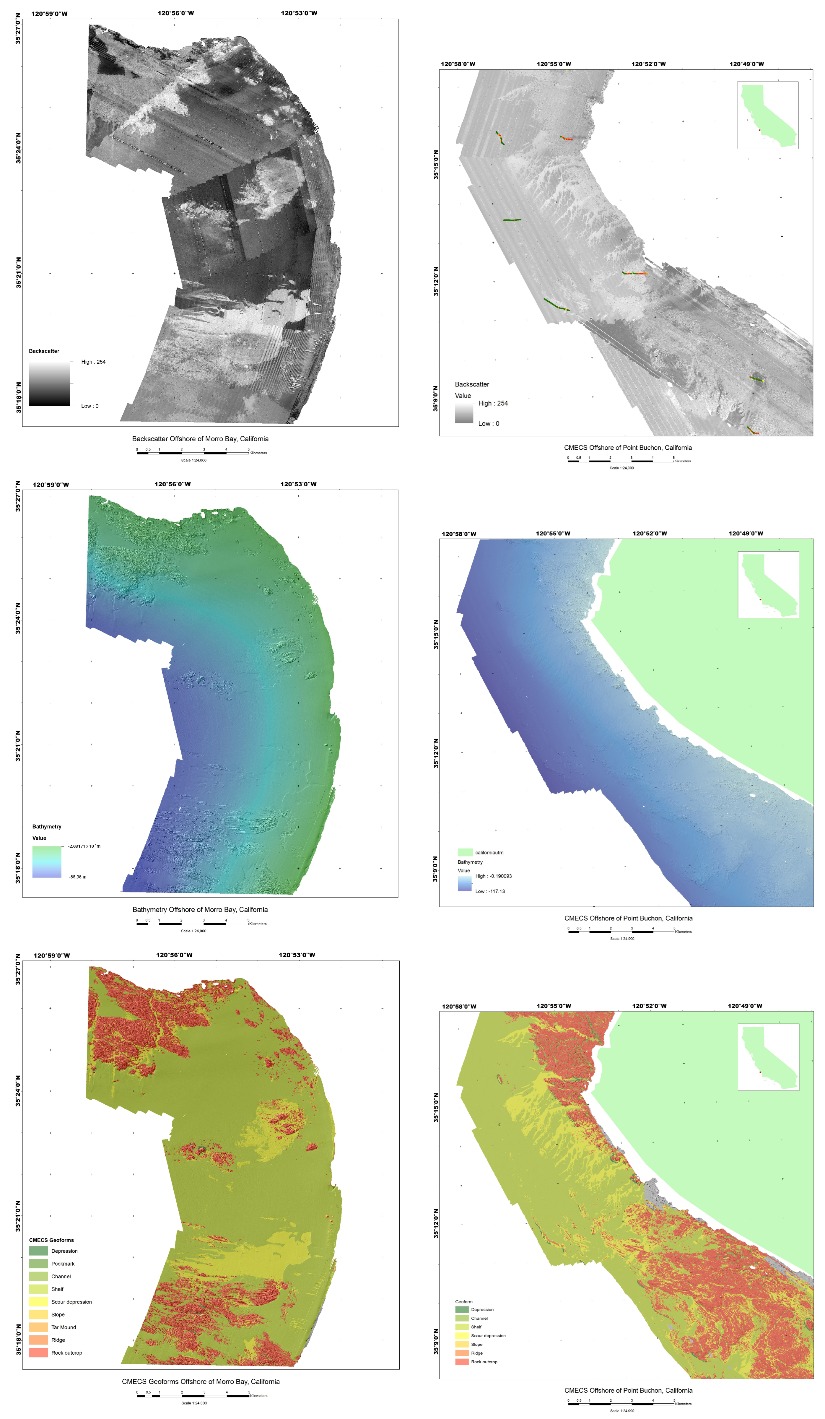
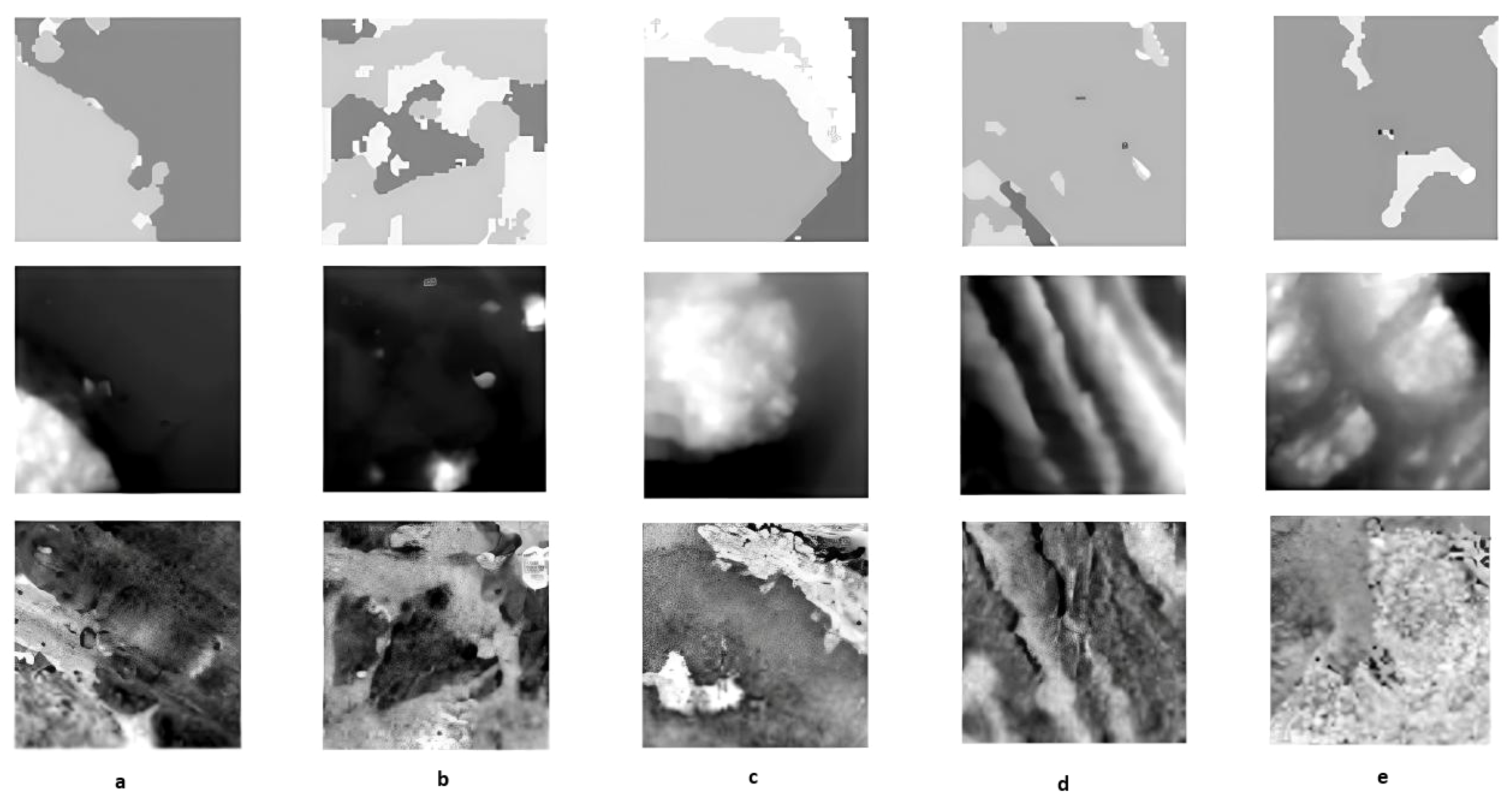
2.1. Dataset

The study area is situated along the California coast, on the Pacific coast of the Western United States, encompassing the offshore waters near Morro Bay (35.37°N, 120.85°W) and Pochon Point (34.72°N, 120.61°W) [61]. The dataset includes panels displaying (from left to right) backscatter data, bathymetric topographic data, and landform category label data, providing a comprehensive representation of the spatial and geological characteristics of each area, which is shown in Figure 1.

After processing, the original multibeam data is divided into three components: backscatter, bathymetric measurements, and geomorphic labels. This data, collected by Fugro Pelagos (San Diego, CA, USA) in 2008, was acquired using multibeam echo sounding systems including the 400-kHz Reson 7125, 240-kHz Reson 8101, and 100-kHz Reson 8111 (Teledyne RESON, Slangerup, Denmark), all providing a 2-meter resolution. The dataset is classified into five main geomorphic categories: continental shelf, rock outcrop, depression, waterway, and ocean ridge (Figure 2). Images are formatted at a resolution of 64 × 64 pixels.

2.2. Models and Methods

The seabed topography is complex and varied, with overlapping and transitional zones between landform types. This diversity results in some boundaries between landforms being blurred or challenging to delineate accurately. In particular, when similar features appear in different geomorphic categories, there is a high degree of inter-class similarity. For example, as shown in Figure 3, the “scour depressions” within the “depressions” category display geomorphologic features that closely resemble those of “waterways”, as both exhibit linear scour patterns. While raised peripheries and concave centers characterize ordinary depressions, scour depressions show high inter-class variability due to frequent tidal erosion, making them even more similar to ‘waterways’. This similarity poses significant challenges for accurately classifying seabed landforms. Therefore, effectively extracting the distinct features of each geomorphic category, establishing relationships between these features, and addressing the high similarity between categories are critical for improving classification accuracy.

We propose a fine-tuning pruned ConDenseNet with label smoothing regularization (LSR) to effectively address these classification challenges, enhancing accuracy and robustness in distinguishing between similar geomorphic categories.

2.2.1. AlexNet, VGG and ResNet

Krizhevsky et al. (2012) [63] introduced AlexNet, a pioneering deep convolutional neural network that achieved a Top-5 error rate of 15.4% on a large-scale image dataset. This network employs the rectified linear unit (ReLU) as the activation function, accelerating model convergence. The dropout mechanism is used to mitigate overfitting, and the GPU replaces the CPU for computation, significantly enhancing training speed.

Simonyan and Zisserman (2014) [64] explored the impact of network depth on CNN performance and developed the Visual Geometry Group (VGG) network, a deep model constructed using simple, repeated building blocks.

Building on the VGG architecture, He et al. [65] addressed the challenge of reduced accuracy with increased network depth by introducing residual blocks, leading to the development of ResNet. By incorporating residual blocks, ResNet allows for creating neural network layers that skip over connections to subsequent layers, reducing the impact of overly strong connections and facilitating the training of much deeper networks. ResNet has demonstrated strong performance and established itself as a benchmark for comparison with subsequent networks, including GoogleNet [66], Inception v3 [67] and v4 [68], MobileNet [69], SqueezeNet [70], and ShuffleNet [71].

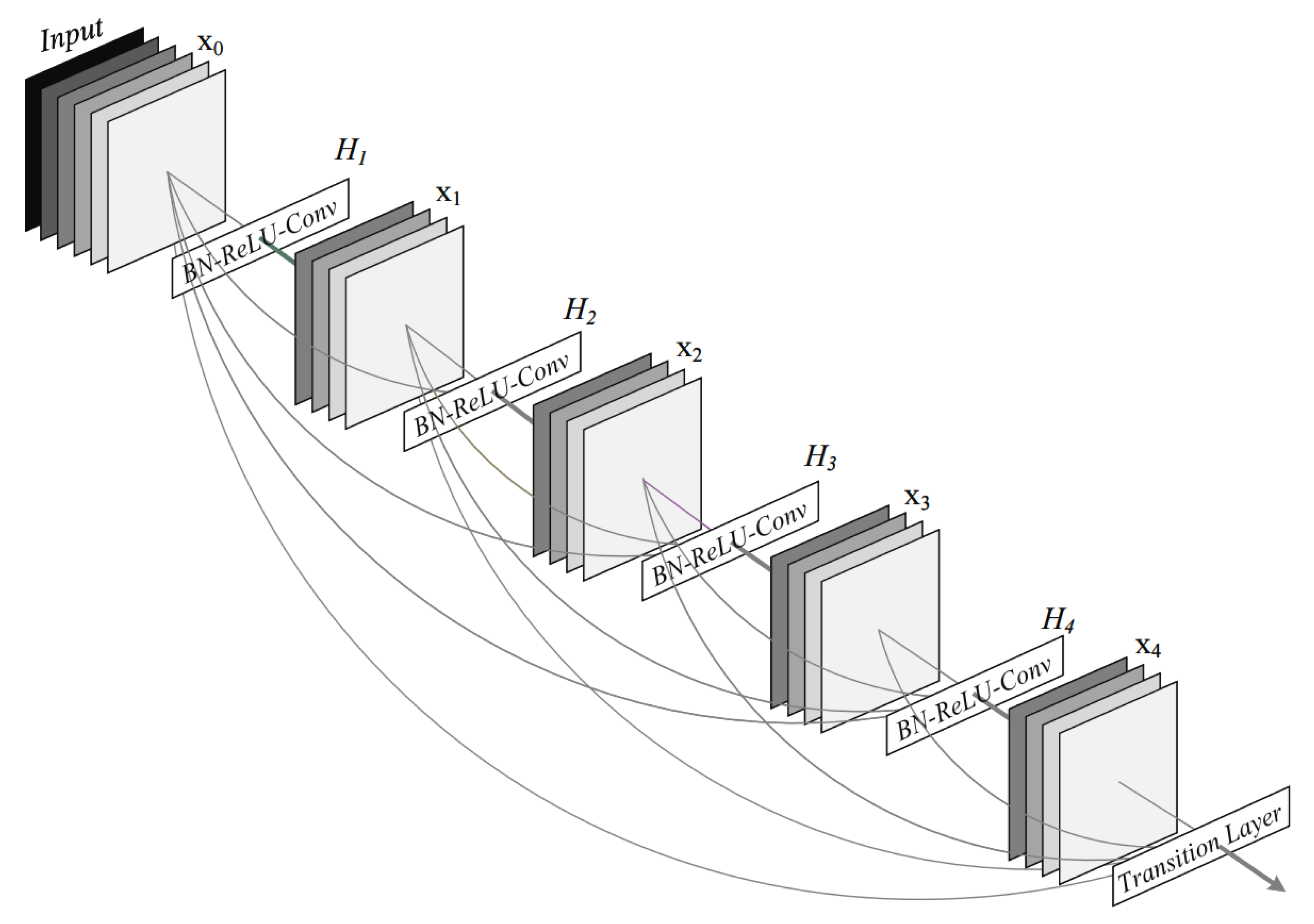
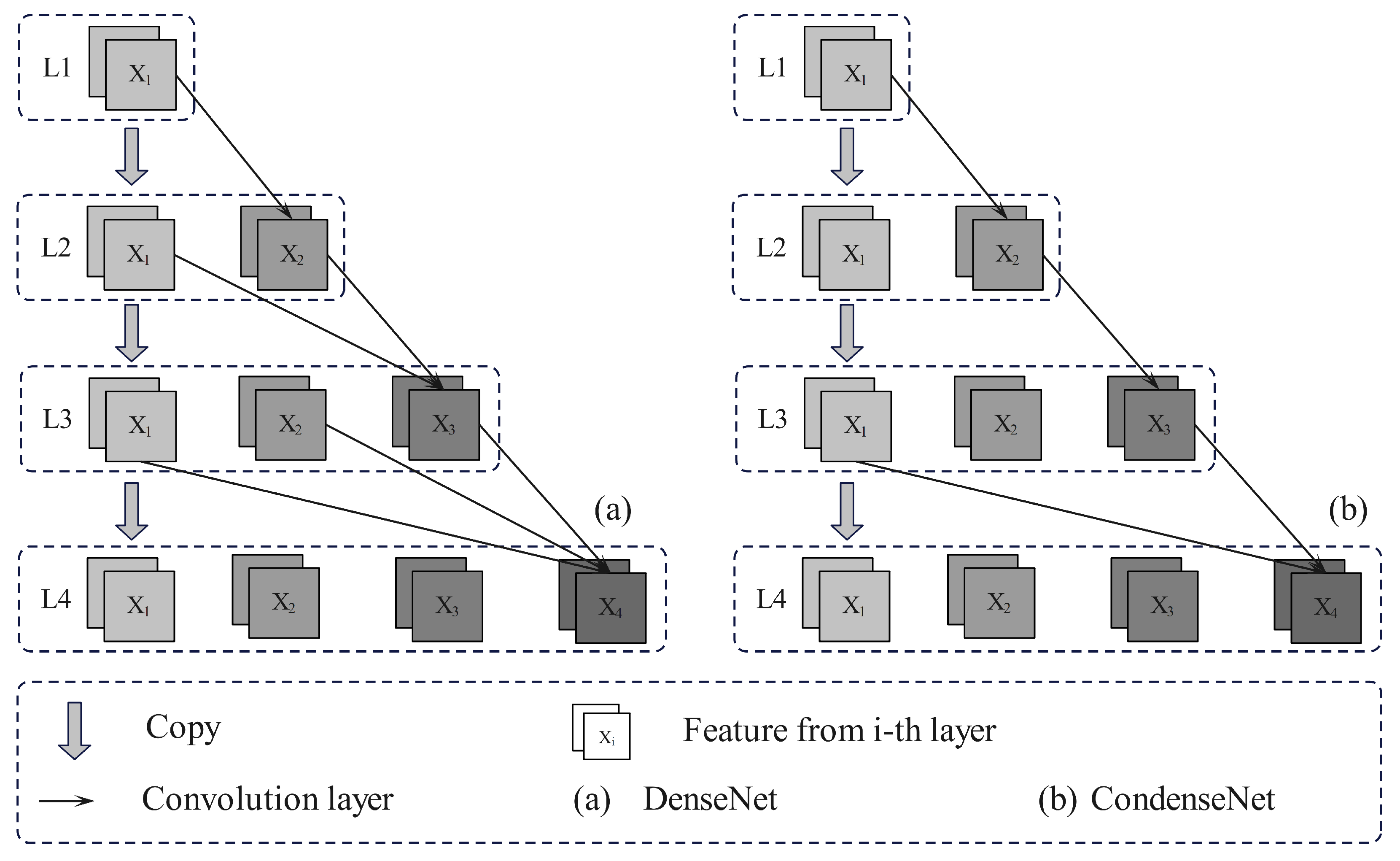
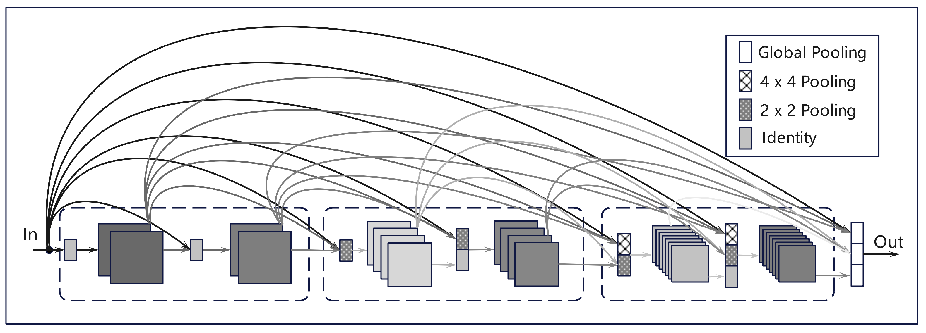
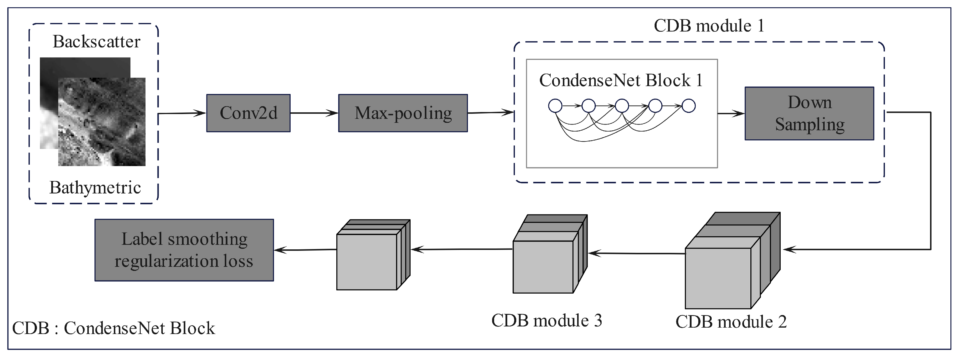
2.2.2. DenseNet and ConDenseNet

Huang et al. (2017) [72] introduced DenseNet, building on the principles of ResNet. Unlike ResNet, DenseNet employs a more radical dense connectivity mechanism, where every layer is connected to all previous layers. Specifically, each layer receives the outputs of all preceding layers as additional inputs as illustrated in Figure 4. This dense connectivity promotes feature reuse, enhancing the network’s efficiency and improving performance by reducing the parameters required to achieve high accuracy. DenseNet achieves comparable accuracy to ResNet on the ImageNet classification dataset while requiring less than half the number of parameters and about one-third of the computational resources to reach the same performance. In DenseNet, the features extracted from each layer serve as nonlinear transformations of the input data (Figure 5), with the complexity of these transformations increasing as the network depth grows (due to the accumulation of nonlinear functions). Unlike traditional neural networks, which rely on the most complex features from the final layer, DenseNet leverages features from earlier layers with lower complexity. This allows DenseNet to create a smoother decision function, leading to better generalization performance. DenseNet exhibits strong resistance to overfitting, making it particularly suitable for datasets with limited samples.

The DenseNet architecture addresses previous challenges by building a deeper, densely connected network. In this network, each hidden layer generates multiple feature maps. DenseNet refers to each hidden layer as a Dense Block (Figure 5), with the number of feature maps (X layers) produced by a layer (H layers) being defined as the growth rate, denoted by the lowercase letter k. For example, when each layer generates four feature maps, k = 4. The dense block, the core component of DenseNet, is designed to maximize information flow between network layers.

In the DenseNet structure, the information added to the network differs significantly from the information retained. Each convolutional layer in a dense block is narrow (e.g., using 12 filters per layer) and only adds a small number of feature maps to the network’s collective knowledge, which are then retained throughout the layers. Unlike traditional network structures, where layers have unidirectional connections, DenseNet employs multiple connections between layers, resulting in $(L+1)/2$ connections for L layers. The convolution operation in the dense block is represented by $x_L=T_L\left(\left[x_0,x_1,\dots ,x_{l-1}\right]\right)$, where $x_0,x_1,$…$,x_{l-1}$ is the convolution layer of the preceding l layer, $x_L$ is the output, and $T_L$ is the set containing nonlinear transformation, including convolution, pooling, and ReLU as illustrated in Figure 6. Each dense block consists of a series of 1 × 1 and 3 × 3 convolution layers with the same padding for cascading operations.

Although DenseNet uses a pattern of dense connections, it requires fewer parameters than traditional convolutional networks. This network structure reduces redundant information learning and minimizes the parameters needed, improving parametric efficiency. Furthermore, the continuous connections between layers allow for faster gradient flow from the raw input data and the loss function, helping mitigate the vanishing gradient problem. This feature reuse method enables the construction of deeper networks to effectively capture the deep semantic relationships between features.

While pre-trained DenseNet effectively identifies complex multivariate data and extracts diverse features, its internal connections may exhibit redundancy. Early features, for example, do not always need to be reused by later layers. To address this, ConDenseNet [73] introduces a pruning operation that specifies the network during training called the Learned Group Convolution (LGC) approach as shown in Figure 7, which is used in pruning to select an optimal pattern of input-output connections, enabling the network to learn which essential features can be pruned automatically. However, due to the complex nature of underwater terrain data, pruning important features could negatively impact the results. During training, convolutional kernels are pruned based on their $L_1$ norm, facilitating group convolution learning. This pruning occurs early in the training process rather than after the model is fully trained, allowing the network weights to be smoothed over time. Compared to DenseNet, ConDenseNet automatically selects the optimal input–output connection mode, ultimately converting the network into a more efficient convolutional structure. The ConDenseNet reduces the computational load to approximately one-tenth while maintaining the same accuracy. The pruning process in ConDenseNet is controlled by the Condensation Procedure parameter across each of its $C_1$ condensing stages, with $1/C$ of weights pruned at each stage. By the end of training, only $1/C$ of the weights in each convolutional group remain, allowing the network to gradually eliminate redundant connections throughout training. This process accurately prunes and smooths the network’s weights, enhancing efficiency. A permute layer is added during training to implement channel interchange, thereby mitigating any adverse effects from the $1\times 1$ LGC layers. This adjustment, performed during training, helps ensure optimal results.

2.2.3. Cross-Entropy Loss Function and Label Smoothing Regularization

Cross-entropy measures the similarity between two probability distributions, p and q, where p represents the true distribution, and q represents an alternative distribution. Cross-entropy quantifies the expected encoding length needed to represent data following the true distribution p but encoded according to q. Specifically, if p is used as the true distribution and q as the alternative, the expected number of bits required to encode an event is represented by $H(p,q)$, defined as Equation (1):

$$H\left(p\right)=\sum _{i}p\left(i\right)·log\left({\displaystyle \frac{1}{p\left(i\right)}}\right)$$

(1)

If the wrong distribution q is used to represent the average encoding length from the true distribution p, then

$$H(p,q)=\sum _{i}p\left(i\right)·log\left({\displaystyle \frac{1}{q\left(i\right)}}\right)$$

(2)

Cross-entropy can be calculated for discrete variables by summing over all classes (Equation (2)); for continuous variables, it requires integration (Equation (3)). In the context of machine learning, cross-entropy serves as a loss function where p represents the distribution of actual labels and q is the distribution of predicted labels from a model. Minimizing cross-entropy loss optimizes the model to align q with p, improving accuracy:

$$-{\int }_{X}P\left(x\right)logQ\left(x\right)dr\left(x\right)=E_p[-logQ]$$

(3)

Label smoothing regularization (LSR), introduced in Rethinking the Inception Architecture for Computer Vision (2016) by Google Brain researchers [67], is a regularization technique designed to prevent models from becoming overly confident during training. It is commonly used for classification tasks to improve generalization and reduce overfitting. Label smoothing replaces “hard” one-hot labels with “soft” labels that assign a small probability to incorrect classes. This modification is achieved by blending one-hot labels with a uniform distribution over all labels, resulting in “smoothed” labels.

For a K-class classification, the one-hot label y is smoothed as Equation (4):

$$y_{\mathrm{smooth}}=(1-\theta )·y+{\displaystyle \frac{\theta }{K}}$$

(4)

where $\theta$ is the smoothing strength. This shift introduces slight uncertainty in the true label, reducing the likelihood of the model becoming too confident about a specific label and encouraging it to generalize better. By reducing the difference between the predicted positive and negative sample outputs, label smoothing improves classification performance, particularly in cases with high-class similarity, as it mitigates overfitting and enhances the model’s adaptability to new data.

Given the importance of LSR, researchers have investigated its effects on training deep neural networks. Müller et al. [74] empirically demonstrated that LSR improves model calibration by making category clusters more compact, increasing the distance between classes, reducing interclass distances, enhancing generalization and improving overall model calibration. For certain tasks, such as classifying submarine landforms, the high similarity between different geomorphic categories introduces challenges in accurate classification. By incorporating label smoothing, the model accounts for cross-entropy in a way that emphasizes correct class predictions while moderating the loss for other classes.

Specifically, LSR can be defined by modifying the standard cross-entropy function as follows in Equation (5):

$$\mathrm{H}\left({\mathrm{q}}^{\prime },\mathrm{p}\right)=(1-\epsilon )ce\left(i\right)+\epsilon \sum {\displaystyle \frac{ce\left(j\right)}{N}}$$

(5)

where $ce\left(i\right)$ represents the standard cross-entropy loss of i, $epsilo$ is a small positive number called the smoothing factor, i is the correct class, and N is the number of classes, uniformly distributed.

From Equation (5), we can find that in the training process, the loss function will consider the loss of the correct category and the loss of other categories. By including the loss of similar categories, the model becomes less susceptible to high interclass similarity, reducing its negative impact on feature representation.

2.2.4. Our Methods: Fine-Tuning Pruned ConDenseNet with Label Smoothing Regulation

We identified a promising synergy within CondenseNet, particularly in its pruning process, which becomes even more effective when combined with the LSR approach. This integration optimizes the cross-entropy loss function for classifying intricate submarine landforms, addressing challenges like interclass similarity with precision.

Our refined method was tested on datasets incorporating backscattering and bathymetric topographic data, utilizing their multi-source potential to boost representational power without substantially increasing model parameters. The input data flows through an initial $7\times 7$ convolutional layer, followed by a $3\times 3$ max-pooling layer, which leads to dense connection layers. Transition layers, equipped with 1 × 1 convolutions and average pooling with a stride of 2, adaptively downsample feature maps. Downsampling occurs three times within the network using CondenseNet’s structure. This strategic design maintains computational efficiency while preserving key spatial features. Finally, the enhanced LSR based cross-entropy loss function minimizes interclass similarity issues, refining feature extraction and significantly improving classification accuracy.

The workflow, visualized in Figure 8, exemplifies how dense network architectures, enriched with label smoothing, handle complex classifications for environmental monitoring, demonstrating their versatility across disciplines with data-intensive challenges.

3. Results

3.1. Comparison Results Across Models

The accuracy evaluation metrics utilized in this study include Precision, Recall, F1-Score, Intersection over Union (IoU), and the confusion matrix. Precision measures the proportion of correctly predicted positive cases out of all predicted positives, calculated as $Precision={\displaystyle \frac{TP}{TP+FP}}$ (TP: true positive; FP: false positive), reflecting the model’s ability to avoid false positives, particularly when evaluating classification performance on actual images. In contrast, Recall (i.e., true positive rate) assesses the proportion of correctly predicted positive cases out of all actual positives, expressed as $Recall={\displaystyle \frac{TP}{TP+FN}}$ (FN: false negative), highlighting the model’s sensitivity to detecting true positives. Precision and Recall often exhibit a trade-off: prioritizing high Precision may lower Recall, and vice versa. While the ideal scenario maximizes both, this is challenging due to their interdependence. To balance this trade-off, the F1-Score, a harmonic mean of Precision and Recall, is commonly used, and a Precision–Recall (P-R) curve can visually represent their relationship across different thresholds. The confusion matrix, or error matrix, provides a standard framework for accuracy assessment.

To demonstrate the effectiveness of our innovative synergy of ConDenseNet with LSR, our approach was tested on California bathymetric topographic data and compared with current mainstream methods such as AlexNet, VGG, ResNet, ViT, and ConDenseNet without LSR.

The dataset was split into training, testing, and validation sets in a 3:1:1 ratio. Ablation experiments were conducted under two distinct scenarios: the first utilized only backscatter data as input, while the second incorporated multisource data, combining backscatter and bathymetric topographic data.

This analysis examines the distribution of correctly and incorrectly classified instances across classes and identifies patterns of misclassification between categories. To ensure robust and reliable results, the dataset was randomly partitioned, and the experiments were repeated 20 times. The final evaluation was based on the mean and standard deviation of overall accuracy across these iterations, reducing the impact of randomness and enhancing the reliability of the results.

From

Table 1. Accuracy comparison between AlexNet, VGG, ResNet, ConDenseNet, ViT, and our approach (ConDenseNet+LSR).

Method	Precision [%]	Recall [%]	F1-Score [%]	IoU
AlexNet	65.46 ± 0.62	39.05 ± 0.78	35.60 ± 0.59	33.28 ± 0.67
VGG	67.87 ± 0.74	38.27 ± 0.82	37.76 ± 0.81	34.43 ± 0.83
ResNet	70.13 ± 0.58	45.77 ± 0.67	45.18 ± 0.73	42.46 ± 0.76
ConDenseNet	71.83 ± 0.84	47.77 ± 0.63	48.62 ± 0.69	40.34 ± 0.68
ViT	61.92 ± 0.38	29.98 ± 0.64	28.60 ± 0.52	31.32 ± 0.42
Our	73.13 ± 0.69	48.40 ± 0.72	54.74 ± 0.63	43.28 ± 0.56

, it is evident that ConDenseNet builds upon the foundational concept of residual connections in ResNet but introduces a more interconnected architecture. While ResNet connects each layer to a limited number of preceding layers (typically 2–3) through element-wise addition, ConDenseNet establishes dense connections by concatenating each layer’s output with all preceding layers along the channel dimension, providing richer inputs for subsequent layers. This dense connectivity not only promotes feature reuse but also enables ConDenseNet to achieve superior performance compared to ResNet, with fewer parameters and reduced computational overhead. However, training ConDenseNet exhibited overfitting issues, likely due to the dense connectivity amplifying noise in the data. By incorporating label smoothing during training, the network’s optimization process became more robust and compact, mitigating overfitting and delivering significantly improved and reliable results.

Figure 9 presents the confusion matrix generated from the classification results of AlexNet, VGG, ResNet, DenseNet, and CondenseNet integrated with the improved LSR with backscatter data only and with both backscatter and bathymetric data. AlexNet, VGG and ResNet all have some failures indicated as blank in Figure 9, e.g., the Ocean ridge. The results indicate that the classification accuracy for the Continental shelf, rock, and depression exceeds 50%, with “shelf” and “depression” achieving notable accuracies of 80% and 83%, respectively. However, other categories exhibit lower classification accuracy, which can be attributed to the relatively smaller sample sizes compared to “shelf” and “depression”. To address this imbalance, future improvements could involve weight adaptation and data augmentation techniques to enhance the model’s ability to classify underrepresented categories.

3.2. Ablation Experiments

To further evaluate each module’s contribution to the proposed network, ablation experiments were conducted using backscatter data as the sole input, which is shown in

Table 2. Ablation experiments of different ConDenseNet variants: without pruning, without LSR, and with both pruning and LSR, on seabed topographic and geomorphic datasets.

Method	Precision [%]	Recall [%]	F1-Score [%]	IoU [%]
ConDenseNet without pruning	71.34 ± 0.56	50.53 ± 0.47	53.28 ± 0.44	35.17 ± 0.35
ConDenseNet without LSR	70.45 ± 0.52	48.43 ± 0.37	52.61 ± 0.55	34.46 ± 0.48
ConDenseNet+LSR	71.74 ± 0.69	50.62 ± 0.72	53.34 ± 0.43	35.28 ± 0.56

. Table 2 compares the classification performance of the entire network and its variants, including configurations without pruning the densely connected network and without improved label smoothing.

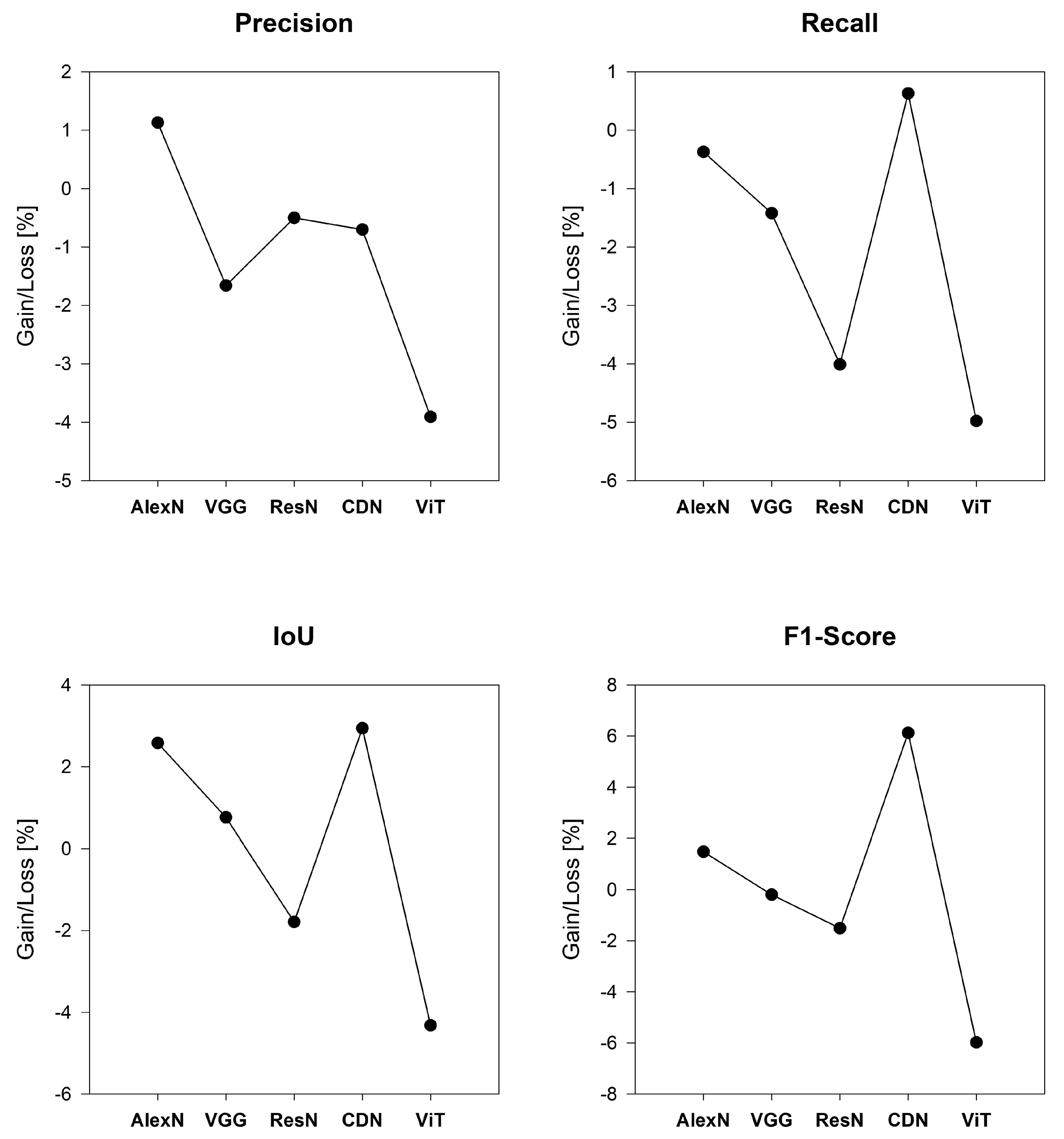
3.3. Different Models Adopt LSR

The LSR had a significant impact on the improvement, but it also seems to be an independent component which may be able to be stripped from our approach. We performed a series of comparisons adopting the LSR with other models, such as AlexNet, VGG, ResNet and ViT with LSR.

The results are shown as

Table 3. Accuracy comparison between AlexNet+LSR, VGG+LSR, ResNet+LSR, ViT+LSR, and our approach (ConDenseNet+LSR).

Method	Precision [%]	Recall [%]	F1-Score [%]	IoU [%]
AlexNet+LSR	66.59 ± 0.56	38.68 ± 0.64	37.08 ± 0.58	35.86 ± 0.56
VGG+LSR	66.21 ± 0.85	36.85 ± 0.37	37.56 ± 0.72	35.19 ± 0.45
ResNet+LSR	69.63 ± 0.23	41.76 ± 0.57	43.67 ± 0.36	40.67 ± 0.38
ViT+LSR	58.92 ± 0.74	25.47 ± 0.43	23.62 ± 0.61	27.58 ± 0.51
ConDenseNet+LSR	73.13 ± 0.69	48.40 ± 0.72	54.74 ± 0.63	36.38 ± 0.56

. This result is better combined with Table 1. We calculated the differences of each model with and without LSR, and the result is illustrated in Figure 10.

4. Discussion

4.1. The Benefit of Adopting Pruned ConDenseNet+LSR (Our Method)

Our method utilizes ConDenseNet as the backbone network, which is pruned and fine-tuned, thereby improving channel selection. It incorporates LSR, which enhances the detection of small objects and reduces overfitting. This design concatenates features across Dense Blocks and employs downsampling through pooling operations to handle varying feature map sizes as illustrated in Figure 9. Furthermore, our approach produces an exponential growth rate, where higher-level features play a crucial role in deeper networks. By increasing the number of channels in later layers, the model achieves greater accuracy, underscoring the significance of feature richness at higher levels.

From Table 1, the results indicate that even without the LSR, our backbone network, ConDenseNet, outperformed most existing methods and demonstrated strong feature extraction capabilities. However, some areas can be improved. The pruning implements the channel selection adaptation, which results in efficiency and flexibility improvement, contributing an additional 0.33% increase in accuracy. That may not sound like much. The pruning would reduce the hyperparameter volume from 4.8 M to about 3 M, as shown in

Table 4. Relative hyperparameter volume and computation time comparison (pruned ConDenseNet as the benchmark).

Method	Parameters	Computation Time	Notes
Pruned ConDenseNet	1× (3 M)	1×	ConDenseNet-121
ConDenseNet	1.6× (4.8 M)	1.5×	ConDenseNet-121
AlexNet	12.7× (61 M)	0.9×
VGG	28× (138 M)	7×	VGG16
ResNet	5.3× (25.6 M)	1.4×	ResNet50
ViT	18× (86 M)	4×	patch = 16
Our	1× (3 M)	1×	Benchmark + LSR

, which cuts about 50% of the computation time. These findings highlight the complementary benefits of pruning and the improved loss function in enhancing the network’s overall classification accuracy. Incorporating the LSR that optimizes the loss function further enhanced classification accuracy by an additional 0.94%. This improvement can be attributed to the loss function’s ability to effectively reduce interclass similarity, particularly among submarine landform and geomorphic categories, thereby refining feature representation. The LSR replaced the standard batch normalization, which provides group normalization and, as a result, better handling of small batch sizes or deployment on edge devices due to the reduction in overfitting. The LSR requires slightly more computation time for all models.

Our proposed approach, which incorporates a fine-tuned pruned ConDenseNet with LSR, achieved a classification accuracy of 71.14%. This outperformed AlexNet, VGG, ResNet, ConDenseNet, and ViT, as shown in Table 1. Specifically, the proposed method achieved approximately 2% higher accuracy than ResNet and nearly 1% higher than ConDenseNet. These results demonstrated the superior classification performance of densely connected networks for submarine topography and geomorphology and demonstrated the effectiveness of the improved label smoothing loss function in mitigating interclass similarity. The improvement might seem marginal in terms of accuracy, but it is worth noting that the F1-score is much higher, at 9.56% and 6.12%, respectively. Our method is also significantly more robust and has a much smaller parameter volume and lower computation time as shown in Table 4. We firmly believe the progress is both solid and meaningful.

4.2. LSR Impact

The general expectation is that LSR can improve the performance of most models we compared and does not cost any significant additional computation time. Our experiences show that all the models with and without LSR have almost the same computation time. However, the impact is not consistent across all equally. Comparing the results from Table 1 and Table 3, we observe that LSR does not always lead to improvements, for example, in VGG, ResNet, and ViT. VGG experienced a precision drop of about 1.66%, and ResNet decreased by approximately 0.5%. For AlexNet, the gain from LSR is marginal at only 1.13%. In contrast, ConDenseNet benefits the most, showing an improvement of around 1.3%. The primary advantages of LSR lie in its ability to mitigate label noise and reduce overfitting, particularly in small-batch training scenarios. That said, it comes at a cost: it introduces additional model complexity and computational overhead, especially in models with large parameter counts like VGG and ViT.

In our experiments, LSR works particularly well when combined with our pruned ConDenseNet. There appears to be a strong synergy between pruning and LSR. While pruning removes redundant channels and simplifies the network, LSR stabilizes the training process and promotes more generalized outputs. Hence, they result in better regularization and more efficient feature learning without sacrificing accuracy. This suggests that the effectiveness of LSR can be amplified when the model architecture is first optimized through structural simplification.

The effects of LSR on AlexNet and VGG were as expected. For AlexNet, the main limitation is its low capacity for generalization, and LSR cannot overcome that fundamental issue. VGG, with its large number of parameters, is already prone to overfitting. Adding LSR in this case seems to make training even more unstable. The performance gains are minimal, while the extra cost in training time and the increased sensitivity to hyperparameters outweigh the benefits. This suggests that LSR may not be suitable for older or deeper architectures that lack built-in regularization.

One interesting point is that both AlexNet ($+1.13\%$) and ConDenseNet ($+1.3\%$) showed small improvements in accuracy with LSR. However, it is important to note that ConDenseNet achieved a much larger improvement in F1-score, with gains of 1.48% (AlexNet) and 6.12% (ConDenseNet). It also performed better in terms of computation time and robustness. Based on these results, we believe it is worthwhile to adopt LSR in ConDenseNet as proposed.

We also expected LSR to integrate well with ResNet. Theoretically, LSR should enhance robustness by reducing overfitting and preventing the model from prematurely locking onto incorrect labels during training, especially important when dealing with high inter-class similarity. However, our results show that precision dropped by approximately 0.5%, and the F1-score declined by about 1.51%. We believe that this is caused by LSR overcompensating for overfitting on our relatively small dataset. This highlights that the benefits of LSR are context-dependent and may require careful calibration based on dataset size and class distribution.

For ViT, it has potential with LSR, but its impact is highly dependent on dataset size. ViT is inherently designed for large datasets through its image-to-token embedding mechanism and dimensionality reduction. When applied to smaller datasets, it tends to underperform due to limited training diversity. In such cases, LSR can serve as a useful regularizer by stabilizing training and mitigating overfitting. However, in our experiments, the benefits were not significant, likely due to the sensitivity of ViT to data volume and its already regularized architecture. A more comprehensive evaluation on larger datasets would be necessary to fully assess the potential of ViT with LSR. It is also worth mentioning the overwhelming computational cost of applying ViT with LSR. It is simply not worth it for small datasets.

5. Conclusions

Seabed landforms exhibit diverse geomorphic features, but their classification poses significant challenges due to the limited amount of available data and the subtle similarities between certain categories, such as depressions and waterways shaped by seawater erosion. Traditional virtual interpretation and existing neural networks struggle to fully extract and differentiate these complex features, leading to suboptimal classification accuracy. Addressing these challenges requires exploring an effective approach that can extract and represent key geomorphic features, establish relationships among them, and enhance classification performance.

This paper proposes a novel fine-tuning pruning ConDenseNet with LSR designed to improve the classification of submarine landforms. Our approach can also incorporate bathymetric terrain data alongside backscatter data as multi-source inputs. The feature space improves the representational power of the input data. Our approach efficiently extracts and connects multi-layered topographic features, while the LSR optimizes the entropy of the loss function, which mitigating overfitting and reducing the impact of interclass similarity on classification results.

Extensive experiments on a custom submarine geomorphic dataset from Morro Bay and Pochon Point, California, demonstrated our approach’s superiority compared to other networks, such as AlexNet, VGG, ResNet, and DenseNet. Our approach achieves higher accuracy with fewer parameters, making it less prone to overfitting. The results validate the effectiveness of label smooth regulation and fine-tuning pruning in capturing essential seabed topographic features, particularly for confusable categories with high interclass similarity.

In conclusion, our proposed fine-tuning pruning ConDenseNet with LSR represents a solid advancement in submarine landform classification, and significantly reduces hyperparameter volume and computation time. It addresses the limitations of traditional interpretation methods and other deep learning approaches, achieving higher precision and robustness in challenging datasets. This approach offers a promising framework for improving geomorphic analysis and advancing research in seabed classification.

In future work, it would be valuable to explore adaptive or dynamic label smoothing techniques that adjust the smoothing factor based on model confidence or learning progress, such as dropout, mixup, or knowledge distillation, which may offer more robust improvements, particularly for models like ResNet and ViT where standard LSR falls short.

We also found that some minority classes, such as “Ocean ridge”, suffered more due to the small sample size from an already limited dataset. We will investigate enhancement approaches to handle such cases, such as adjusting class weights or applying data augmentation.

References

1. Mittal, S.; Srivastava, S.; Jayanth, J.P. A Survey of Deep Learning Techniques for Underwater Image Classification. IEEE Trans. Neural Netw. Learn. Syst. 2023, 34, 6968–6982. [Google Scholar] [CrossRef]
2. Micallef, A.; Krastel, S.; Savini, A. Submarine Geomorphology; Springer: Berlin/Heidelberg, Germany, 2017. [Google Scholar]
3. Sowers, D.C.; Masetti, G.; Mayer, L.A.; Johnson, P.; Gardner, J.V. Standardized geomorphic classification of seafloor within the United States Atlantic canyons and continental margin. Front. Mar. Sci. 2020, 7, 9. [Google Scholar] [CrossRef]
4. Witze, A. Diving deep: The centuries-long quest to explore the deepest ocean. Nature 2023, 616, 653. [Google Scholar] [CrossRef] [PubMed]
5. Vesnaver, A.; Baradello, L. Sea Floor Characterization by Multiples’ Amplitudes in Monochannel Surveys. J. Mar. Sci. Eng. 2023, 11, 1662. [Google Scholar] [CrossRef]
6. Nikiforov, S.; Ananiev, R.; Jakobsson, M.; Moroz, E.; Sokolov, S.; Sorokhtin, N.; Dmitrevsky, N.; Sukhikh, E.; Chickiryov, I.; Zarayskaya, Y.; et al. The Extent of Glaciation in the Pechora Sea, Eurasian Arctic, Based on Submarine Glacial Landforms. Geosciences 2023, 13, 53. [Google Scholar] [CrossRef]
7. Wilson, K.; Mohrig, D. Signatures of Pleistocene Marine Transgression Preserved in Lithified Coastal Dune Morphology of The Bahamas. Geosciences 2023, 13, 367. [Google Scholar] [CrossRef]
8. Li, J.; Xing, Q.; Tian, L.; Hou, Y.; Zheng, X.; Arif, M.; Li, L.; Jiang, S.; Cai, J.; Chen, J.; et al. An Improved UAV RGB Image Processing Method for Quantitative Remote Sensing of Marine Green Macroalgae. IEEE J. Sel. Top. Appl. Earth Obs. Remote Sens. 2024, 17, 19864–19883. [Google Scholar] [CrossRef]
9. Principi, S.; Palma, F.; Bran, D.M.; Bozzano, G.; Isola, J.; Ormazabal, J.; Esteban, F.; Acosta, L.Y.; Tassone, A. Seafloor geomorphology of the northern Argentine continental slope at 40–41° S mapped from high-resolution bathymetry. J. S. Am. Earth Sci. 2023, 134, 104748. [Google Scholar] [CrossRef]
10. Kruss, A.; Rucinska, M.; Grzadziel, A.; Waz, M.; Pocwiardowski, P. Multi-band, calibrated backscatter from high frequency multibeam systems as an efficient tool for seabed monitoring. In Proceedings of the 2023 IEEE Underwater Technology (UT), Tokyo, Japan, 6–9 March 2023; pp. 1–5. [Google Scholar] [CrossRef]
11. Zhang, F.; Zhuge, J. Modeling and Solving of Seafloor Terrain Detection Based on Multibeam Bathymetr. In Proceedings of the 2024 IEEE 3rd International Conference on Electrical Engineering, Big Data and Algorithms (EEBDA), Changchun, China, 27–29 February 2024; pp. 235–241. [Google Scholar] [CrossRef]
12. Millar, D.; Mitchell, G.; Brumley, K. How Modern Multibeam Surveys Can Dramatically Increase Our Understanding of the Seafloor and Waters Above to Support the United Nations Decade of Ocean Science for Sustainable Development. In Proceedings of the OCEANS 2019 MTS/IEEE SEATTLE, Seattle, WA, USA, 27–31 October 2019; pp. 1–5. [Google Scholar] [CrossRef]
13. Van Dijk, T.A.G.P.; Roche, M.; Lurton, X.; Fezzani, R.; Simmons, S.M.; Gastauer, S.; Fietzek, P.; Mesdag, C.; Berger, L.; Klein Breteler, M.; et al. Bottom and Suspended Sediment Backscatter Measurements in a Flume—Towards Quantitative Bed and Water Column Properties. J. Mar. Sci. Eng. 2024, 12, 609. [Google Scholar] [CrossRef]
14. Anokye, M.; Cui, X.; Yang, F.; Wang, P.; Sun, Y.; Ma, H.; Amoako, E.O. Optimizing multi-classifier fusion for seabed sediment classification using machine learning. Int. J. Digit. Earth 2023, 17, 2295988. [Google Scholar] [CrossRef]
15. Liu, Y.; Wu, Z.; Zhao, D.; Zhou, J.; Shang, J.; Wang, M.; Zhu, C.; Luo, X. Construction of High-Resolution Bathymetric Dataset for the Mariana Trench. IEEE Access 2019, 7, 142441–142450. [Google Scholar] [CrossRef]
16. Wang, J.; Tang, Y.; Jin, S.; Bian, G.; Zhao, X.; Peng, C. A Method for Multi-Beam Bathymetric Surveys in Unfamiliar Waters Based on the AUV Constant-Depth Mode. J. Mar. Sci. Eng. 2023, 11, 1466. [Google Scholar] [CrossRef]
17. de Andrade Neto, W.P.; Paz, I.D.S.R.; Oliveira, R.A.A.C.E.; De Paulo, M.C.M. Comparison of the vertical accuracy of satellite-based correction service and the PPK GNSS method for obtaining sensor positions on a multibeam bathymetric survey. Sci. Rep. 2024, 14, 11104. [Google Scholar] [CrossRef]
18. Shang, X.; Dong, L.; Zhao, J. Optimal Scale Determination for Object-Based Backscatter Image Analysis in Seafloor Substrate Classification Based on Classification Uncertainty. IEEE Geosci. Remote Sens. Lett. 2024, 21, 1501005. [Google Scholar] [CrossRef]
19. Orange, D.L.; Teas, P.A.; Decker, J.; Gharib, J. Use of multibeam bathymetry and backscatter to improve seabed geochemical surveys—Part 1: Historical review, technical description, and best practices. Interpretation 2023, 11, T215–T247. [Google Scholar] [CrossRef]
20. Grządziel, A. The Impact of Side-Scan Sonar Resolution and Acoustic Shadow Phenomenon on the Quality of Sonar Imagery and Data Interpretation Capabilities. Remote Sens. 2023, 15, 5599. [Google Scholar] [CrossRef]
21. Guo, J.; Zhang, Z.; Wang, M.; Ma, P.; Gao, W.; Liu, X. Automatic Detection of Subsidence Funnels in Large-Scale SAR Interferograms Based on an Improved-YOLOv8 Model. IEEE Trans. Geosci. Remote Sens. 2024, 62, 6200117. [Google Scholar] [CrossRef]
22. Wang, K. The Application Of Acoustic Detection Technology In The Investigation Of Submarine Pipelines. J. Appl. Sci. Eng. 2024, 27, 2981–2991. [Google Scholar]
23. Wang, D.; Chen, G.; Chen, J.; Cheng, Q. Seismic data denoising using a self-supervised deep learning network. Math. Geosci. 2024, 56, 487–510. [Google Scholar] [CrossRef]
24. Zhou, Q.; Li, X.; Zheng, J.; Li, X.; Kan, G.; Liu, B. Inversion of Sub-Bottom Profile Based on the Sediment Acoustic Empirical Relationship in the Northern South China Sea. Remote Sens. 2024, 16, 631. [Google Scholar] [CrossRef]
25. Jamieson, J.W.; Gini, C.; Brown, C.; Robert, K. Interferometric synthetic aperture sonar: A new tool for seafloor characterization. In Frontiers in Ocean Observing: Marine Protected Areas, Western Boundary Currents, and the Deep Sea; Kappel, E.S., Cullen, V., Coward, G., da Silveira, I.C.A., Edwards, C., Morris, T., Roughan, M., Eds.; Oceanography 38 (Supplement 1); The Oceanography Society: Rockville, MD, USA, 2025; pp. 86–88. [Google Scholar] [CrossRef]
26. Gerg, I.D.; Cook, D.A.; Monga, V. Adaptive Phase Learning: Enhancing SyntheticAperture Sonar Imagery Through Learned Coherent Autofocus. IEEE J. Sel. Appl. Earth Obs. Remote Sens. 2024, 17, 9517–9532. [Google Scholar] [CrossRef]
27. Mann, S.; Novellino, A.; Hussain, E.; Grebby, S.; Bateson, L.; Capsey, A.; Marsh, S. Coastal Sediment Grain Size Estimates on Gravel Beaches Using Satellite Synthetic Aperture Radar (SAR). Remote Sens. 2024, 16, 1763. [Google Scholar] [CrossRef]
28. Yang, P. An imaging algorithm for high-resolution imaging sonar system. Multimed. Tools Appl. 2024, 83, 31957–31973. [Google Scholar] [CrossRef]
29. Bauer, P.; Hoefler, T.; Stevens, B.; Hazeleger, W. Digital twins of Earth and the computing challenge of human interaction. Nat. Comput. Sci. 2024, 4, 154–157. [Google Scholar] [CrossRef] [PubMed]
30. Vance, T.C.; Huang, T.; Butler, K.A. Big data in Earth science: Emerging practice and promise. Science 2024, 383, eadh9607. [Google Scholar] [CrossRef]
31. Gerhardinger, L.C.; Colonese, A.C.; Martini, R.G.; da Silveira, I.; Zivian, A.; Herbst, D.F.; Glavovic, G.B.; Calvo, S.T.; Christie, P. Networked media and information ocean literacy: A transformative approach for UN ocean decade. npj Ocean Sustain. 2024, 3, 2. [Google Scholar] [CrossRef]
32. Fu, C.; Liu, R.; Fan, X.; Chen, P.; Fu, H.; Yuan, W.; Zhu, M.; Luo, Z. Rethinking general underwater object detection: Datasets, challenges, and solutions. Neurocomputing 2023, 517, 243–256. [Google Scholar] [CrossRef]
33. Guan, M.; Xu, H.; Jiang, G.; Yu, M.; Chen, Y.; Luo, T.; Zhang, X. DiffWater: Underwater Image Enhancement Based on Conditional Denoising Diffusion Probabilistic Model. IEEE J. Sel. Top. Appl. Earth Obs. Remote Sens. 2024, 17, 2319–2335. [Google Scholar] [CrossRef]
34. Deng, Y.; Tang, S.; Chang, S.; Zhang, H.; Liu, D.; Wang, W. A Novel Scheme for Range Ambiguity Suppression of Spaceborne SAR Based on Underdetermined Blind Source Separation. IEEE Trans. Geosci. Remote Sens. 2025, 63, 5207915. [Google Scholar] [CrossRef]
35. Chen, J.; Zhang, S. Segmentation of sonar image on seafloor sediments based on multiclass SVM. J. Coast. Res. 2018, 83, 597–602. Available online: https://www.jstor.org/stable/26543022 (accessed on 27 July 2025). [CrossRef]
36. Liu, H.; Xu, K.; Li, B.; Han, Y.; Li, G. Sediment Identification Using Machine Learning Classifiers in a Mixed-Texture Dredge Pit of Louisiana Shelf for Coastal Restoration. Water 2019, 11, 1257. [Google Scholar] [CrossRef]
37. Ji, X.; Yang, B.; Tang, Q. Seabed sediment classification using multibeam backscatter data based on the selecting optimal random forest model. Appl. Acoust. 2020, 167, 107387. [Google Scholar] [CrossRef]
38. Sheykhmousa, M.; Mahdianpari, M.; Ghanbari, H. Support Vector Machine Versus Random Forest for Remote Sensing Image Classification: A Meta-Analysis and Systematic Review. IEEE J. Sel. Top. Appl. Earth Obs. Remote Sens. 2020, 13, 6308–6325. [Google Scholar] [CrossRef]
39. Ouyang, S.; Xu, J.; Chen, W.; Dong, Y.; Li, X.; Li, J. A Fine-Grained Genetic Landform Classification Network Based on Multimodal Feature Extraction and Regional Geological Context. IEEE Trans. Geosci. Remote Sens. 2022, 60, 4511914. [Google Scholar] [CrossRef]
40. Tran, H.T.T.; Nguyen, Q.H.; Pham, T.H.; Ngo, G.T.H.; Pham, N.T.D.; Pham, T.G.; Tran, C.T.M.; Ha, T.N. Novel Learning of Bathymetry from Landsat 9 Imagery Using Machine Learning, Feature Extraction and Meta-Heuristic Optimization in a Shallow Turbid Lagoon. Geosciences 2024, 14, 130. [Google Scholar] [CrossRef]
41. Chen, G.; Kusky, T.; Luo, L.; Li, Q.; Cheng, Q. Hadean tectonics: Insights from machine learning. Geology 2023, 51, 718–722. [Google Scholar] [CrossRef]
42. Cui, X.; Yang, F.; Wang, X.; Ai, B.; Luo, Y.; Ma, D. Deep learning model for seabed sediment classification based on fuzzy ranking feature optimization. Mar. Geol. 2020, 432, 106390. [Google Scholar] [CrossRef]
43. Zhu, Z.; Fu, X.; Hu, Y. A Sonar image recognition method using transfer learning to train Convolutional neural networks. J. Unmanned Underw. Syst. 2020, 28, 89–96. (In Chinese) [Google Scholar] [CrossRef]
44. Wan, J.; Qin, Z.; Cui, X.; Yang, F.; Yasir, M.; Ma, B.; Liu, X. MBES Seabed Sediment Classification Based on a Decision Fusion Method Using Deep Learning Model. Remote Sens. 2022, 14, 3708. [Google Scholar] [CrossRef]
45. Dai, Z.; Liang, H.; Duan, T. Small-Sample Sonar Image Classification Based on Deep Learning. J. Mar. Sci. Eng. 2022, 10, 1820. [Google Scholar] [CrossRef]
46. Qin, X.; Luo, Z.; Wu, J.; Shang, J.; Zhao, D. Deep Learning-Based High Accuracy Bottom Tracking on 1-D Side-Scan Sonar Data. IEEE Geosci. Remote Sens. Lett. 2022, 19, 8011005. [Google Scholar] [CrossRef]
47. Jiao, W.; Zhang, J. Sonar Images Classification While Facing Long-Tail and Few-Shot. IEEE Trans. Geosci. Remote Sens. 2022, 60, 1–20. [Google Scholar] [CrossRef]
48. Arosio, R.; Hobley, B.; Wheeler, A.J.; Sacchetti, F.; Conti, L. A,; Furey, T.; Lim, A. Fully convolutional neural networks applied to large-scale marine morphology mapping. Front. Mar. Sci. 2023, 10, 1228867. [Google Scholar] [CrossRef]
49. Du, X.; Sun, Y.; Song, Y.; Dong, L.; Zhao, X. Revealing the Potential of Deep Learning for Detecting Submarine Pipelines in Side-Scan Sonar Images: An Investigation of Pre-Training Datasets. Remote Sens. 2023, 15, 4873. [Google Scholar] [CrossRef]
50. Anokye, M.; Cui, X.; Yang, F.; Fan, M.; Luo, Y.; Liu, H. CNN multibeam seabed sediment classification combined with a novel feature optimization method. Math. Geosci. 2024, 56, 279–302. [Google Scholar] [CrossRef]
51. Huang, J.; Song, W.; Liu, T.; Cui, X.; Yan, J.; Wang, X. Submarine Landslide Identification Based on Improved DeepLabv3 with Spatial and Channel Attention. Remote Sens. 2024, 16, 4205. [Google Scholar] [CrossRef]
52. Xie, C.; Chen, P.; Zhang, S.; Huang, H. Nearshore Bathymetry from ICESat-2 LiDAR and Sentinel-2 Imagery Datasets Using Physics-Informed CNN. Remote Sens. 2024, 16, 511. [Google Scholar] [CrossRef]
53. Qiu, L.; Zhu, C.; Guo, J.; Yang, L.; Li, W. Enhanced Deep-Learning Method for Marine Gravity Recovery From Altimetry and Bathymetry Data. IEEE Geosci. Remote Sens. Lett. 2024, 21, 1501805. [Google Scholar] [CrossRef]
54. Geisz, J.K.; Wernette, P.A.; Esselman, P.C. Classification of Lakebed Geologic Substrate in Autonomously Collected Benthic Imagery Using Machine Learning. Remote Sens. 2024, 16, 1264. [Google Scholar] [CrossRef]
55. Meng, J.; Yan, J.; Zhang, Q. Anti-Interference Bottom Detection Method of Multibeam Echosounders Based on Deep Learning Models. Remote Sens. 2024, 16, 530. [Google Scholar] [CrossRef]
56. Sun, K.; Wu, Z.; Wang, M.; Shang, J.; Liu, Z.; Zhao, D.; Luo, X. Accurate Identification Method of Small-Size Polymetallic Nodules Based on Seafloor Hyperspectral Data. J. Mar. Sci. Eng. 2024, 12, 333. [Google Scholar] [CrossRef]
57. Ruan, B.; Shuai, H.; Cheng, W. Vision Transformers: State of the Art and Research Challenges, Computer Vision and Pattern Recognition. arXiv 2022. [Google Scholar] [CrossRef]
58. Wang, H.; Li, X. DeepBlue: Advanced convolutional neural network applications for ocean remote sensing. IEEE Geosci. Remote Sens. Mag. 2024, 12, 138–161. [Google Scholar] [CrossRef]
59. Zavala-Romero, O.; Bozec, A.; Chassignet, E.P.; Miranda, J.R. Convolutional neural networks for sea surface data assimilation in operational ocean models: Test case in the Gulf of Mexico. Ocean Sci. 2025, 21, 113–132. [Google Scholar] [CrossRef]
60. Wang, N.; Wang, A.Y.; Joo, M. Review on deep learning techniques for marine object recognition: Architectures and algorithms. Control Eng. Pract. 2022, 118, 104458. [Google Scholar] [CrossRef]
61. Cochrane, G.R.; Cole, A.; Sherrier, M.; Roca-Lezra, A. Bathymetry, Backscatter Intensity, and Benthic Habitat Offshore of Morro Bay, California (ver. 1.1, January 2024): U.S. Geological Survey Data Release. 2022. Available online: https://cmgds.marine.usgs.gov/data-releases/datarelease/10.5066-P9HEZNRO/ (accessed on 27 July 2025).
62. Zhao, X.; Wang, L.; Zhang, Y.; Han, X.; Deveci, M.; Parmar, M. A review of convolutional neural networks in computer vision. Artif. Intell. Rev. 2024, 57, 99. [Google Scholar] [CrossRef]
63. Krizhevsky, A.; Sutskever, I.; Hinton, G.E. Imagenet classification with deep convolutional neural networks. In Proceedings of the Advances in Neural Information Processing Systems 25 (NIPS 2012), Lake Tahoe, NV, USA, 3–6 December 2012. [Google Scholar]
64. Simonyan, K.; Zisserman, A. Very Deep Convolutional Networks for Large-Scale Image Recognition. arXiv 2014, arXiv:1409.1556. [Google Scholar]
65. He, K.; Zhang, X.; Ren, S.; Sun, J. Deep Residual Learning for Image Recognition. arXiv 2015, arXiv:1512.03385. [Google Scholar]
66. Szegedy, C.; Liu, W.; Jia, Y.; Sermanet, P.; Reed, S.; Anguelov, D.; Erhan, D.; Vanhoucke, V.; Rabinovich, A. Going deeper with convolutions. In Proceedings of the IEEE Conference on Computer Vision and Pattern Recognition, Boston, MA, USA, 7–12 June 2015; pp. 1–9. [Google Scholar]
67. Szegedy, C.; Vanhoucke, V.; Ioffe, S.; Shlens, J.; Wojna, Z. Rethinking the inception architecture for computer vision. In Proceedings of the IEEE Conference on Computer Vision and Pattern Recognition, Las Vegas, NV, USA, 27–30 June 2016; pp. 2818–2826. [Google Scholar]
68. Szegedy, C.; Ioffe, S.; Vanhoucke, V.; Alemi, A. Inception-v4, inception ResNet and the impact of residual connections on learning. In Proceedings of the AAAI Conference on Artificial Intelligence, San Francisco, CA, USA, 4–9 February 2017; Volume 31. [Google Scholar]
69. Howard, A.G.; Zhu, M.; Chen, B.; Kalenichenko, D.; Wang, W.; Weyand, T.; Andreetto, M.; Adam, H. MobileNets: Efficient convolutional neural networks for mobile vision application. arXiv 2017, arXiv:1704.04861. [Google Scholar]
70. Iandola, F.N.; Han, S.; Moskewicz, M.W.; Ashraf, K.; Dally, W.J.; Keutzer, K. SqueezeNet: AlexNet-level accuracy with 50x fewer parameters and <0.5 MB model size. arXiv 2016, arXiv:1602.07360. [Google Scholar]
71. Zhang, X.; Zhou, X.; Lin, M.; Sun, J. ShuffleNet: An extremely efficient convolutional neural network for mobile devices. In Proceedings of the IEEE Conference on Computer Vision and Pattern Recognition, Salt Lake City, UT, USA, 18–23 June 2018; pp. 6848–6856. [Google Scholar]
72. Huang, G.; Liu, Z.; Van Der Maaten, L.; Weinberger, K.Q. Densely connected convolutional networks. In Proceedings of the IEEE Conference on Computer Vision and Pattern Recognition, Honolulu, HI, USA, 21–26 July 2017; pp. 4700–4708. [Google Scholar]
73. Huang, G.; Liu, S.; Van der Maaten, L.; Weinberger, K.Q. CondenseNet: An Efficient DenseNet using Learned Group Convolutions. Group 2017, 3, 11. [Google Scholar]
74. Müller, R.; Kornblith, S.; Hinton, E.G. When Does Label Smoothing Help. arXiv 2019, arXiv:1906.02629. [Google Scholar]
Figure 1. The dataset includes panels displaying (from top to bottom) backscatter data, bathymetric topographic data, and landform category label data, Morro Bay (left) and Point Buchon (right).
Remotesensing 17 02686 g001
Figure 2. Seabed classification samples: (a) Continental shelf, (b) Rock, (c) Depression, (d) Waterway, (e) Ocean ridge. All images are formatted with a 64 × 64 pixel size.
Remotesensing 17 02686 g002
Figure 3. Inter-class similarity sample: the “scour depressions” (a) display geomorphological features close to “waterways” (b).
Remotesensing 17 02686 g003
Figure 4. The brief structure of DenseNet, where X i are the concatenated feature layers and H i are the transform outputs layers.
Remotesensing 17 02686 g004
Figure 5. Schematic diagram of dense block module, where each previous feature layer ( X i layer) contributes to all the rest of the layers.
Remotesensing 17 02686 g005
Figure 6. Dense block and condense block during training/testing (where X i represents the features of layer i, downward arrows indicate feature map replication, L i multiple connections between layers, and oblique arrows represent convolution layers).
Remotesensing 17 02686 g006
Figure 7. ConDenseNet network structure diagram.
Remotesensing 17 02686 g007
Figure 8. Schematic diagram of a densely connected network based on LSR.
Remotesensing 17 02686 g008
Figure 9. The confusion matrix of AlexNet, VGG, ResNet (Top, left to right) and DenseNet, ConDenseNet with LSR with Backscatter data only and with Backscatter and bathymetric data (Bottom, left to right). (0) Continental shelf, (1) Rock, (2) Depression, (3) Waterway, (4) Ocean ridge.
Remotesensing 17 02686 g009
Figure 10. The gain/loss plots of AlexNet (AlexN), VGG, ResNet (ResN), ConDenseNet (CDN) and ViT with and without LSR in Precision, Recall, IoU and F1-Score.
Remotesensing 17 02686 g010