Induced Polarization Imaging: A Geophysical Tool for the Identification of Unmarked Graves

Abstract

The identification of unmarked graves is important in archaeology, forensics, and cemetery management, but invasive methods are often restricted due to ethical or cultural concerns. This necessitates the use of non-invasive geophysical techniques. Our study demonstrates the potential of induced polarization (IP) imaging as a non-invasive remote sensing technique specifically suited for detecting and characterizing unmarked graves. IP leverages changes in the electrical properties of soil and pore water, influenced by the accumulation of organic matter from decomposition processes. Measurements were conducted at an inactive cemetery using non-invasive textile electrodes to map a documented grave from the early 1990s, with a survey design optimized for high spatial resolution. The results reveal a distinct polarizable anomaly at a 0.75–1.0 m depth with phase shifts exceeding 12 mrad, attributed to organic carbon from wooden burial boxes, and a plume-shaped conductive anomaly indicating the migration of dissolved organic matter. While electrical conductivity alone yielded diffuse grave boundaries, the polarization response sharply delineated the grave, aligning with photographic documentation. These findings underscore the value of IP imaging as a non-invasive, data-driven approach for the accurate localization and characterization of graves. The methodology presented here offers a promising new tool for archaeological prospection and forensic search operations, expanding the geophysical toolkit available for remote sensing in culturally and legally sensitive contexts.

1. Introduction

In historical and archaeological research, unmarked graves offer valuable insights into past societies, conflicts, and burial practices (e.g., [1,2]). At the intersection of forensics and archaeology, locating unmarked graves is essential for uncovering historical events and providing closure to affected communities (e.g., [2,3,4]).

The use of direct investigations, i.e., based on invasive methods, might be prohibited for examining particular protected areas, e.g., due to religious or traditional concerns [5]. This demands the development and application of alternative non-invasive approaches to respect cultural and legal constraints. Forensic geoscience has proven to be effective in investigating various types of burial sites, offering valuable insights without disturbing the ground (see [6] for a review). Remote sensing methods such as light detection and ranging (LiDAR) (see [7] for a recent review), multispectral imaging (e.g., [8,9]), and thermal imaging (e.g., [8,10]) provide valuable information, yet their depth of investigation is usually limited to the uppermost tens of centimeters of the subsurface. Forensic geophysics expands the depth of investigation to several meters using sensors deployed on the ground surface. The increased depth of investigation and the scalable spatial resolution provided by near-surface geophysical methods are the main advantages over remote sensing techniques and are critical for the detection of burials located at larger depths.

Archaeological and forensic investigations employ a variety of geophysical methods depending on site-specific conditions and objectives (e.g., [11,12]). Magnetic surveys measure variations in the Earth’s magnetic field caused by buried ferrous materials, making them effective for locating burned structures, hearths, or graves with magnetic contrasts [13,14]. However, their effectiveness can be limited in areas with weak magnetic contrasts or modern metal debris. Electromagnetic induction (EMI) methods operating in the kHz range measure changes in bulk soil conductivity and magnetic susceptibility, allowing for the detection of buried metallic objects, disturbed soils, and variations in sediment composition [15]. Their relatively fast survey times make EMI methods increasingly attractive for large-scale mapping, yet the vertical resolution of the data might be limited (e.g., [16]). Ground-penetrating radar (GPR) relies on high-frequency electromagnetic (EM) wave reflections to image subsurface structures, enabling the detection of unmarked graves, buried remains, and architectural features (e.g., [3,17,18,19,20,21,22,23,24,25,26,27]). The method assumes that graves or other anomalies produce contrasts in dielectric properties relative to the surrounding soil. While GPR provides high-resolution imaging, its applicability in media with high electrical conductivity (e.g., wet clay-rich soils) is limited due to the attenuation of EM waves reducing the depth of investigation and resolution, respectively (e.g., [28]).

The electrical resistivity tomography (ERT) is based on current injection through galvanic contact between the device and the soil using metal bars and produces 2D or 3D images of the electrical conductivity of the subsurface. The depth of investigation and resolution are controlled by the separation and number of electrodes (e.g., [29]), while the detectability of natural or artificial anomalies also depends on contrasts in the electrical properties of the surrounding medium and the target (e.g., [30]). Successful applications of ERT have been reported for the investigation of cemeteries (e.g., [31,32]), homicides or cold cases [33,34], and crimes committed during conflicts and wars (e.g., [3,35,36,37,38]). Several studies have used simulated (clandestine) graves to investigate grave-related signatures in electrical resistivity data (e.g., [20,39,40,41,42]). Additionally, research has focused on the long-term evolution of these signatures in response to the decomposition process (e.g., [9,43,44,45,46]). The main factor for variations in the electrical properties was found to be the release of conductive fluids associated with the decomposition process (e.g., [32,43,47,48]). Recent forensic research has addressed the monitoring of decomposition fluid migration in the subsurface through geophysical methods, e.g., using GPR [49]. However, the spatial and temporal detectability of graves relies on the contrast between their physical properties and those of the geological media. Hence, results depend on site-specific conditions [50], and the detection of burials might be possible even after the decomposition process is finished (e.g., [41]). In particular, the interpretation of ERT results may be challenging to discriminate between an increase in the electrical conductivity response due to changes in fluid conductivity, clay content or other lithological changes (e.g., [51]).

The induced polarization (IP) method is an extension of the ERT that offers the potential to differentiate materials with a high surface charge and area associated with the polarization of charges in the electrical double layer (EDL) formed at the grain–pore fluid interface (e.g., [52,53,54]). Hence, the IP method is sensitive to variations in sediment compaction and the presence of organic materials, and it allows us to discriminate between air-filled and rocky soils. Recent studies have demonstrated that the IP effect is sensitive to changes in total organic carbon (TOC; e.g., [55,56]), thus highlighting the potential of IP to delineate the increased amount of organic matter in clandestine graves. IP has been applied in controlled (outdoor) crime scene facilities (e.g., [57]) and forensic investigations (e.g., [37]), yet to our knowledge, no contemporary peer-reviewed studies have utilized the IP method specifically for grave identification.

In this study, we propose IP measurements as a remote sensing approach for identifying and characterizing graves. Specifically, our approach leverages the polarization effect associated with organic matter adsorbed to soil particles and an increase in electrical conductivity indicating dissolved organic matter in the electrolyte, enhancing fluid conductivity. Our investigation is conducted at an inactive cemetery, where a grave established in the early 1990s is well documented in terms of location and shape, providing a unique opportunity to evaluate the technique under realistic conditions. To accommodate ethical and religious constraints, our IP measurements use textile electrodes that allow for a non-invasive galvanic coupling to the soil [58,59]. In particular, this study presents three key contributions: (1) a novel quantitative approach to assess the influence of microtopography on geophysical data and inversion, enabling improved survey design and interpretation; (2) the first application of the IP method for the detection and characterization of clandestine graves, advancing forensic geophysics; and (3) a practical survey strategy employing non-invasive textile electrodes suitable for sensitive study areas.

2. Materials and Methods

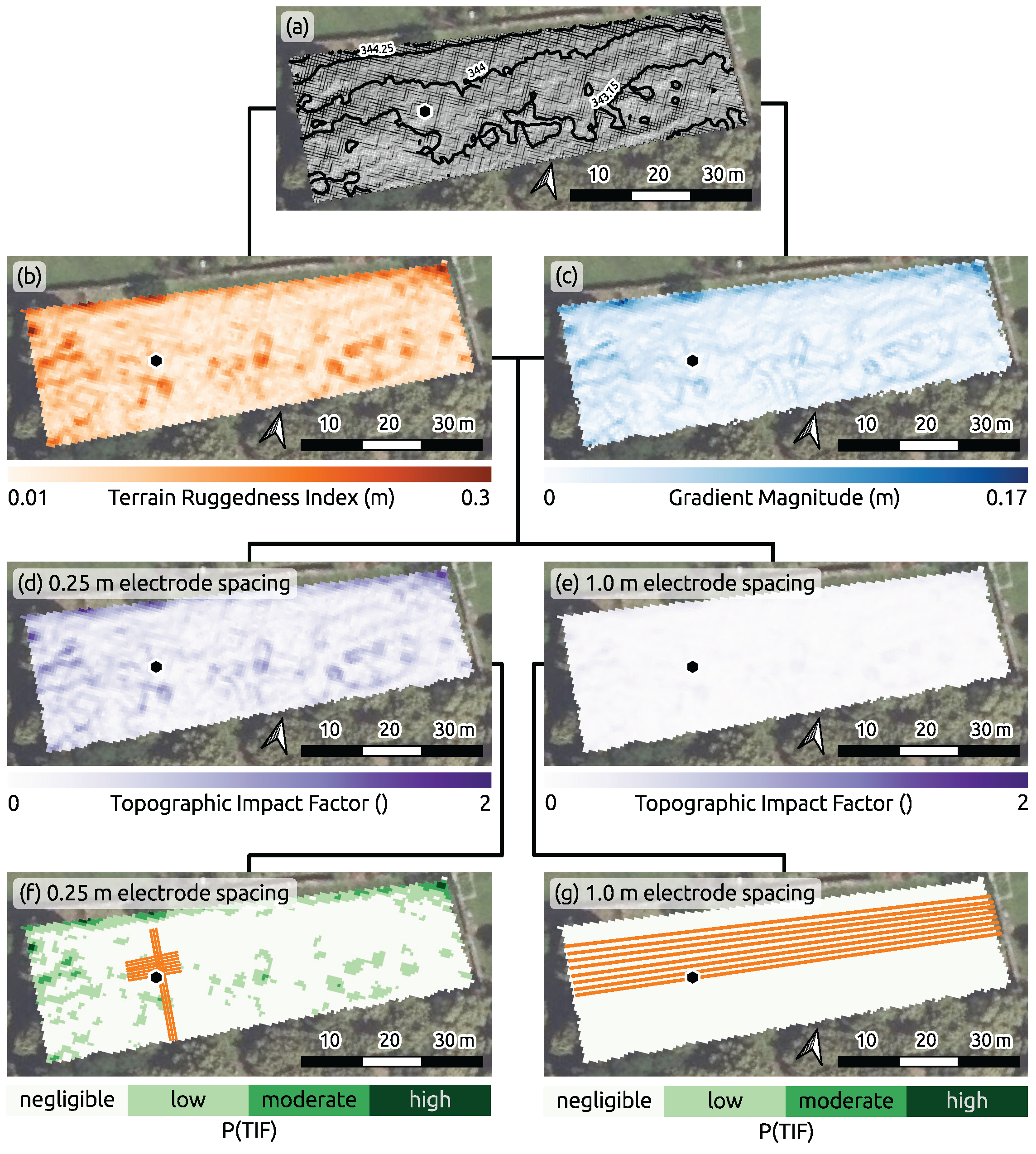
2.1. Novel Strategy for Forensic Geophysical Investigations Using the Induced Polarization Method

To adhere to ethical or religious requirements, we developed a strategy for geophysical electrical investigations at cemeteries based on textile electrodes recently proposed by a team of researchers from TU Braunschweig [58,59]. A textile electrode consists of a sand bag wrapped in an electrically conductive fabric. This design establishes a galvanic contact between the electrode and the soil without the need to introduce metal rods into the ground, as can be seen in Figure 1. Bast el al. [60] demonstrated that textile electrodes are a reliable and accurate alternative to conventional steel electrodes for ERT measurements, offering advantages in terms of contact resistance, reciprocal error, and field logistics, among other performance metrics.

For our experiments, we connected the textile electrodes to unshielded multi-core electrode cables using conventional pegs, which proved to be an effective and cost-efficient mechanism that still follows recommendations of Flores Orozco et al. [61] regarding EM coupling. By connecting the electrode cables to the central control unit, current supplied by an external 12 V battery can be injected into the subsurface. In this study, we used a Syscal Pro Switch from IRIS Instruments (Orléans, France) as the control unit for measurements with up to 72 electrodes that facilitates current injections of up to 2.5 A at voltages up to 800 V. With 10 simultaneous voltage measurements at microvolt resolution, data collection is possible even in environments characterized by materials with high electrical resistivity.

With the Syscal Pro Switch, induced polarization (IP) measurements are conducted in the time-domain, i.e., based on the injection of direct current (DC) into the subsurface through the current electrodes A and B. The resulting potential is measured with a second pair of electrodes, namely the potential electrodes M and N (by convention), referring to the conventional electrical resistivity (ER) measurements. The IP method expands on this approach by measuring the voltage decay curve after the current injection has been turned off. For imaging applications, hundreds to thousands of four-electrode (ABMN) readings are collected with tens of electrodes deployed in 2D or 3D survey geometries.

The inversion of IP imaging datasets solves for models of the subsurface’s electrical properties, i.e., images of the variations in the complex conductivity (CC). The CC is represented by the symbol ${\sigma }^{\ast }$ and can be expressed in terms of the real and imaginary components (${\sigma }^{\prime }$ and ${\sigma }^{″}$, respectively) or in terms of its magnitude $\left|\sigma \right|=\sqrt{{\sigma }^{\prime 2}+{\sigma }^{″2}}$ and phase $\phi =ta{n}^{-1}=\left({\sigma }^{\prime }/{\sigma }^{″}\right)$ as

$${\sigma }^{\ast }={\sigma }^{\prime }+i{\sigma }^{″}=\left|\sigma \right|e^{i\phi },$$

(1)

where $i=\sqrt{-1}$ is the imaginary unit. In Equation (1), the real and imaginary components of the CC refer to the conductive and capacitive properties of the subsurface materials, respectively.

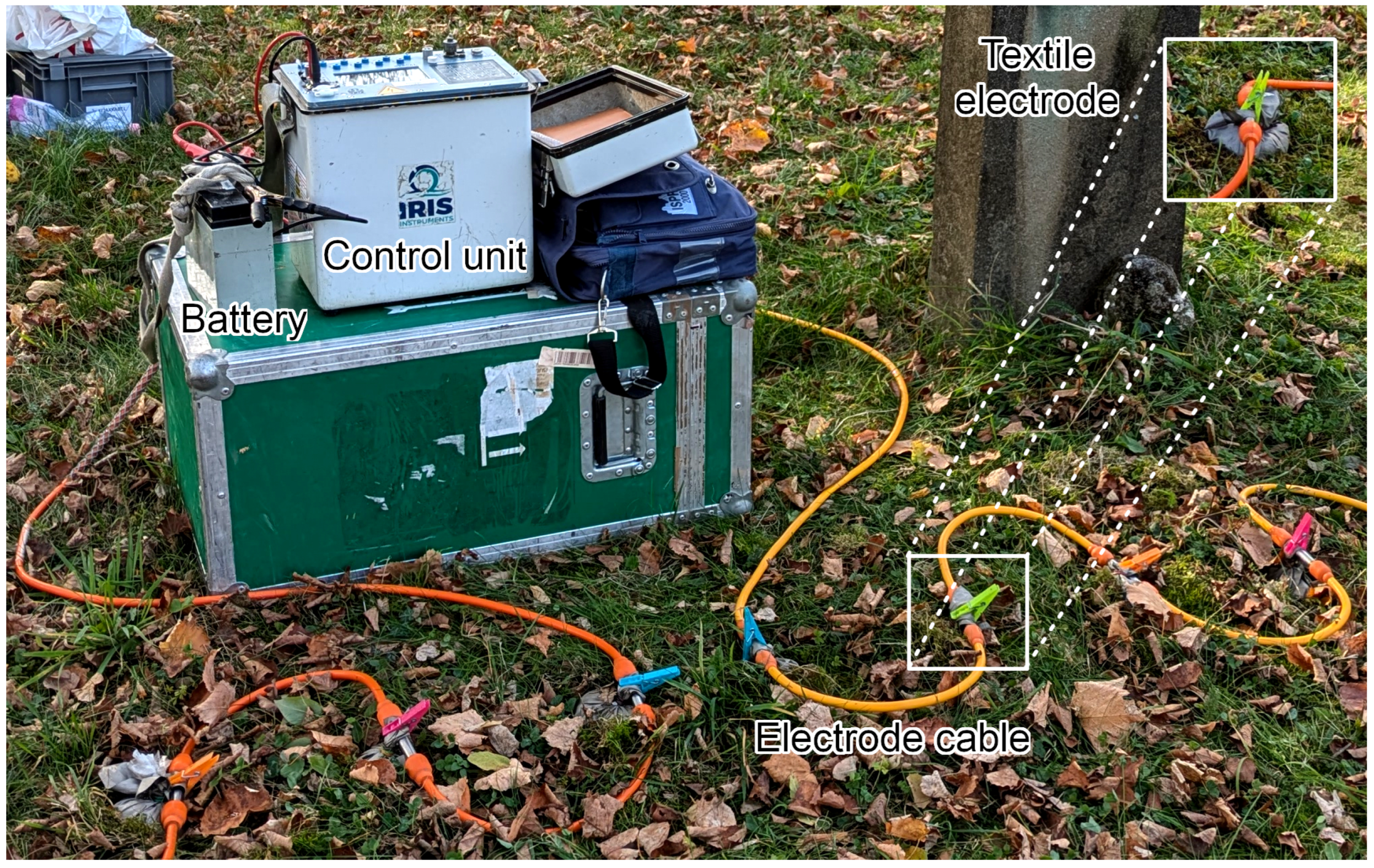
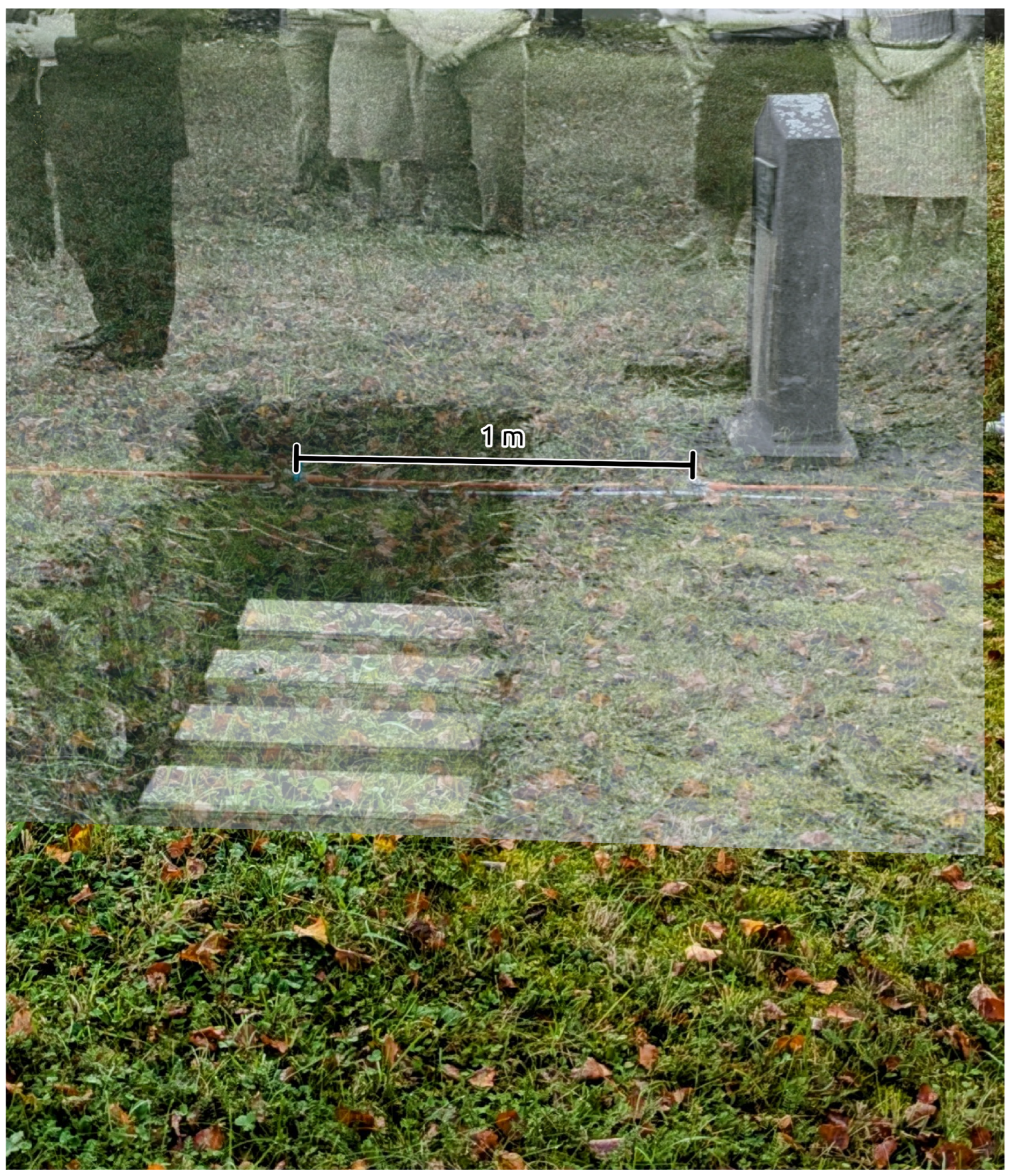
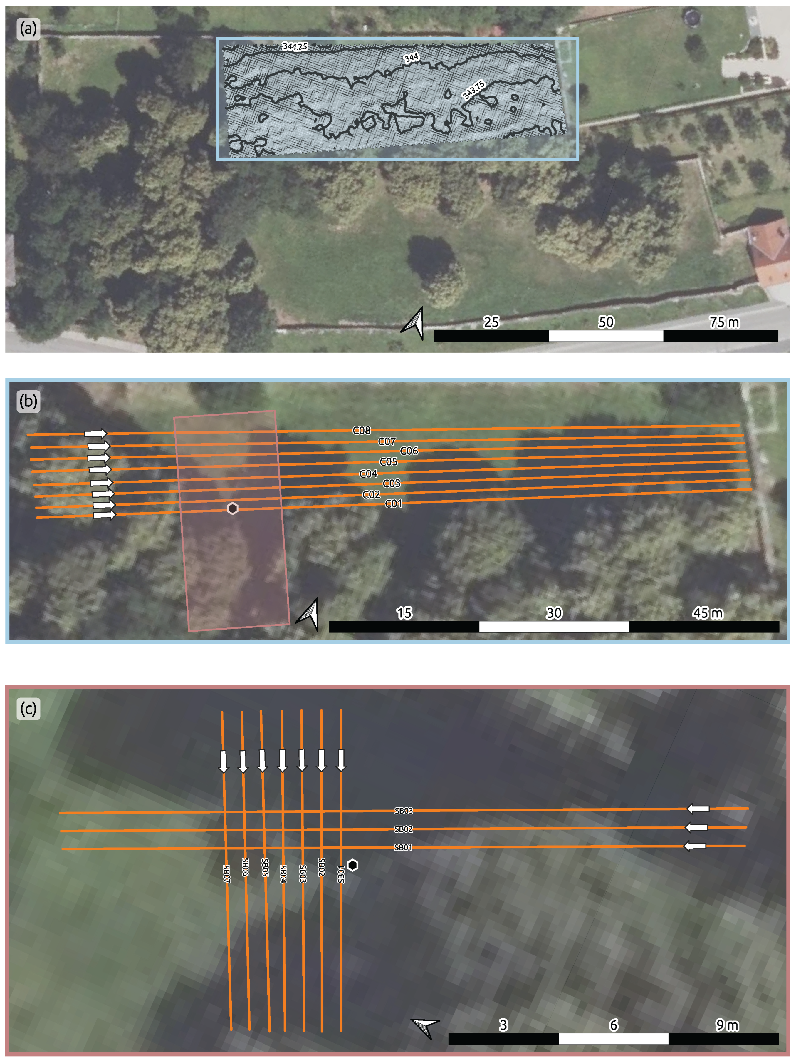
2.2. Collection of Induced Polarization (IP) Data at an Inactive Cemetery

The study was conducted at an inactive cemetery that has not been in use for several decades. The soil conditions at the site are predominantly clayey, which supports the application of the IP method, as its depth of investigation is not significantly affected by the clay fraction in the soil. A key aspect of this investigation is the availability of photographic documentation of a burial that took place under special circumstances in the early 1990s, which served as a reference for assessing the effectiveness of the IP method in grave detection. This photograph provides well-defined control points that enable alignment with a contemporary photograph of the same location. A composite representation was created by overlaying the two images (Figure 2), providing an approximate reference for the grave’s location in the present-day cemetery. This documentation was instrumental in guiding the survey design and selecting measurement locations. It is important to note that drilling and soil sampling were prohibited within the study area; therefore, photographic evidence served as a key reference for evaluating the IP imaging results.

We collected IP data along 18 profiles within the northern sector of the cemetery (Figure 3). A large-scale survey was performed, with an electrode spacing of 1.0 m aimed at achieving an optimal balance between depth of investigation and areal coverage. This survey geometry enabled the detection of broader conductivity variations to depths down to approximately 2.0 m, appropriate for characterizing subsurface conditions across the presumed grave-free area. For the detailed investigation surrounding the known burial, a small electrode spacing of 0.25 m was used. This resolution was selected to resolve subsurface features with expected vertical extents of up to 75 cm, ensuring sufficient spatial sampling to capture the burial geometry and associated heterogeneities within the upper 1.0 m of the subsurface. The selection of electrode spacings reflects an explicit trade-off: the 1.0 m spacing facilitates greater depth of investigation at the expense of spatial resolution, while the 0.25 m spacing prioritizes detailed imaging at shallower depths, necessary for precise grave characterization.

IP data were acquired with a Syscal Pro Switch system, which includes a low-pass digital filter at 10 Hz that defines the upper bound of the frequency content of the data. For data acquisition, a pulse length of 500 ms was applied (fundamental frequency about 2 Hz), with chargeability recorded between 20 ms and 500 ms after the current was switched off. Measurements were captured using 19 sampling gates of 20 ms each. We employed a dipole–dipole (DD) electrode configuration with skip-3 and skip-0 measurements (i.e., dipole lengths of 1 and 4 times the electrode spacing) to balance depth penetration and near-surface resolution.

We refer the reader to Flores Orozco et al. [62] for further details on the measurement configuration.

2.3. Subsurface Descretization for the Geophysical Inversion

As shown in Figure 3a, the IP data were collected in an area of the cemetery characterized by an overall elevation change of approximately 0.5 m, indicating a generally flat topography. However, considering the small electrode spacing of 0.25 and 1.0 m, short-range elevation changes may still influence the geophysical data and the inversion. Therefore, a comparison between the digital elevation model (DEM) and the geophysical survey design is crucial to assess whether microtopographic variations introduce significant effects. We devised an approach that allows us to quantitatively justify the assumption of flat topography in the inversion of the IP data, rather than relying solely on visual inspection of the DEM or survey profiles. The corresponding workflow is summarized in the flowchart presented in Figure 4.

To assess the roughness or ruggedness of the surface, we computed the Terrain Ruggedness Index (TRI; see Figure 5b). We follow the approach of Riley et al. [63] that computes the TRI for a pixel at $\left(i,j\right)$ of the DEM as

$$TRI\left(i,j\right)=\sqrt{\sum _{i=k}^8{\left(z_k-z\left(i,j\right)\right)}^2},$$

(2)

where $z\left(i,j\right)$ is the elevation value of the central pixel, and $z_k$ represents the elevation values of the eight neighboring pixels around the pixel at $\left(i,j\right)$. The TRI map obtained for our study presented in Figure 5b shows localized strong elevation changes in the order of the electrode spacings.

To account for the terrain steepness, we compute the partial derivatives in the x- and y-direction, i.e., the gradient of the DEM, as

$$\begin{array}{c}\hfill {\displaystyle \frac{\partial z}{\partial x}}={\displaystyle \frac{z\left(i+1,j\right)-z\left(i-1,j\right)}{2r}}\end{array}$$

(3)

$$\begin{array}{c}\hfill {\displaystyle \frac{\partial z}{\partial y}}={\displaystyle \frac{z\left(i,j+1\right)-z\left(i,j-1\right)}{2r}},\end{array}$$

(4)

where $z\left(i,j\right)$ is the elevation at pixel $\left(i,j\right)$, and r denotes the DEM resolution, i.e., the pixel size in meters. Based on the partial derivatives, we compute the gradient magnitude $|\nabla z|$ as

$$|\nabla z|=r\sqrt{{\left({\displaystyle \frac{\partial z}{\partial x}}\right)}^2+{\left({\displaystyle \frac{\partial z}{\partial y}}\right)}^2},$$

(5)

where the multiplication by r ensures that the gradient magnitude is given in meters. As can be seen in Figure 5c, the gradient magnitude within the study area is smaller than the electrode spacing and evidences the overall flatness of the area.

We combine TRI and $|\nabla z|$ to obtain the Topographic Impact Factor (TIF) for a given sensor spacing s as

$$TIF={\displaystyle \frac{TRI+|\nabla z|}{s}}.$$

(6)

We consider the TIF a quantitative measure for the impact of the topography in the study area on the geophysical data and inversion depending on the spatial resolution of the investigations, i.e., the electrode spacing. The distinct ranges of TIF values for 0.25 and 1.0 m electrode spacings presented in Figure 5d and e illustrate the need for a further processing step to allow for an objective evaluation of the TIF.

To this end, we apply an S-curve classification approach to the resolved TIF maps to compute the probability of the topographic impact on the inversion process, respectively:

$$P\left(TIF\right)={\displaystyle \frac{1}{1+e^{-k\left(TIF-TI{F}_0\right)}}}.$$

(7)

In Equation (7), k controls the sharpness of the transition around $TI{F}_0$, with $TI{F}_0=1$ as the transition point at which the topography starts to become substantial with respect to the sensor spacing.

The categorized probability maps presented in Figure 5f and g suggest that for the electrode spacings of 0.25 and 1.0 m, the topographic variations in the study area have a negligible-to-low impact on the geophysical data or the inversion process. Accordingly, we consider a flat topography for the modeling and inversion of the IP data.

2.4. Resolving 3D Models of the Subsurface Electrical Properties

To process the IP datasets, we applied the decay curve analysis method described by Flores Orozco et al. [62]. The integral chargeability values derived from the time-domain IP measurements were transformed into impedance phase values through a linear conversion, allowing for inversion in terms of complex resistivity [64]. The transformation is necessary to resolve both conductive and capacitive electrical properties, but it relies on the assumption of a constant phase value, thereby neglecting potential frequency-dependent effects [65]. The effective bandwidth of the IP data collected in this study, ranging from 2 to 10 Hz, is too narrow to meaningfully assess frequency dependence in the IP response. Consequently, the assumption of a constant phase value is considered valid within this limited frequency range. Based on this assumption, the conversion of the measured integral chargeability values to apparent phase values using a linear relationship is appropriate. Moreover, the interpretation of the IP imaging results in this study is qualitative and centers on the spatial mapping of anomalous features rather than a quantitative characterization of subsurface material properties such as organic carbon content. Even if the linear conversion introduces minor uncertainties in the calculated phase values, these do not affect the interpretation or conclusions of the study.

The inversion of the filtered IP data allows us to resolve 3D models of the subsurface conductive and capacitive properties. In particular, the geophysical inversion estimates a model $\mathbf{m}$ that best explains the observed data ${\mathbf{d}}_{obs}$ (here, resistance R and impedance phase shift $\phi$). This is achieved by minimizing an objective function consisting of a data misfit term ${\Psi }_d$ and a regularization term ${\Psi }_m$ [66,67]:

$$\Psi \left(\mathbf{m}\right)={\Psi }_d\left(\mathbf{m}\right)+\lambda {\Psi }_m\left(\mathbf{m}\right),$$

(8)

where the regularization parameter $\lambda$ balances the relative influence of the data misfit and the model roughness [67]. The data misfit term in Equation (8) quantifies the discrepancy between observed and predicted data, ensuring that the inversion process seeks a model consistent with the given measurements:

$${\Psi }_d\left(\mathbf{m}\right)={\Vert {\displaystyle \frac{1}{ϵ}}\left({\mathbf{d}}_{obs}-{\mathbf{d}}_{mod}\right)\Vert }_2^2,$$

(9)

where $ϵ$ denotes the error model accounting for uncertainties arising from measurement noise and modeling inaccuracies, i.e., systematical errors need to be removed prior to the inversion. The proper estimation of $ϵ$ is essential—underestimating may lead to overfitting, while overestimating it can produce overly smooth or unrealistic models (e.g., [52,66]).

The inversion process terminates when a predefined data-fit criterion is met or when changes in the objective function $\Psi$ stabilize (e.g., [66,67]). A common measure for assessing the data misfit is the error-weighted chi-squared fit [66,68]:

$${\chi }^2={\displaystyle \frac{{\Psi }_d}{D}},$$

(10)

where D refers to the length of the data vector $\mathbf{d}$. In a least-squares framework, the inversion is considered converged when ${\chi }^2\approx 1$, indicating that the model explains the data within the assumed error bounds (e.g., [66,67]). Solutions with $1\le {\chi }^2\le 5$ may still be acceptable (e.g., [52,66]).

In this study, we use the pyGIMLi (v1.3.1) framework [69] to conduct a two-step inversion approach: (1) A resistivity inversion is performed using a smoothness-constrained least-squares method to obtain a stable resistivity model. (2) Once the resistivity model is obtained, it is fixed as a reference for the inversion of the impedance phase shift data, ensuring that the IP response is recovered independently (e.g., [70]).

Table 1. Inversion and convergence parameters for the 3D inversion of geophysical data collected with 1.0 m (dataset LI) and 0.25 m (dataset DI) electrode spacing.

	Parameter	Unit	LI	DI
Regularization	$\lambda$	-	200	50
	${\mathrm{z}}_{Weight}$	-	0.1	0.1
Error model	${\mathrm{Err}}_{\sigma }$	%	$5/100$	$5/100$
	${\mathrm{Err}}_{\varphi }$	rad	$1/1000$	$3/1000$
Convergence	${\chi }_{\sigma }^2$	-	2.56	4.18
	${\chi }_{\varphi }^2$	-	2.27	0.94

summarizes inversion parameters (e.g., error models and regularization settings) and convergence parameters for the datasets processed in this study, providing insight into the stability and reliability of the inversion results.

3. Results

We present the induced polarization (IP) imaging results as depth slices extracted from 3D subsurface models. This approach facilitates interpretation by highlighting spatial patterns that may be linked to natural or anthropogenic features. To achieve consistency in our analysis, both the large-scale investigation (LI) and the detailed investigation (DI) are visualized using an identical colormap and colorbar limits (Figure 6 and Figure 7). To ensure the reliability of the presented results, areas with low sensitivity—where the geophysical inversion is poorly constrained due to limited data coverage or unfavorable model geometry—are systematically blanked in the visualizations. These areas, where data resolution is inadequate to reliably constrain model parameters, are omitted from the depth slices to avoid interpretation of poorly resolved features.

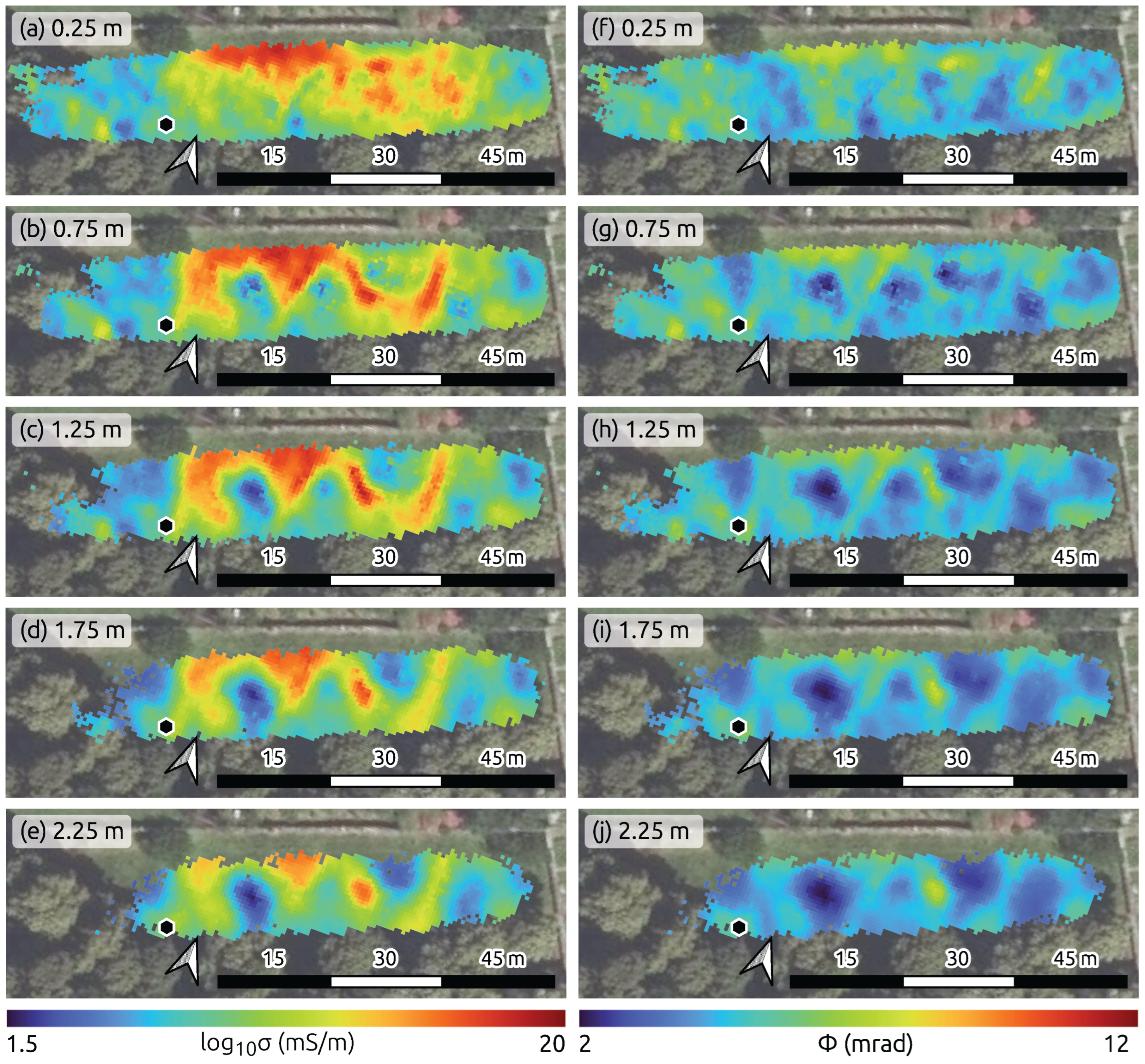
3.1. Large-Scale Investigation (LI) of Subsurface Conditions Within the Area of Interest

The large-scale investigation provides insight into the general subsurface conditions down to a depth of 2.25 m. Depth slices at 0.25, 0.75, 1.25, 1.75, and 2.25 m through the 3D models of the electrical conductivity $\sigma$ (Figure 6a–e) and the polarization effect (represented by the phase $\varphi$ of the complex conductivity; Figure 6f–j) reveal a heterogeneous near-surface composition. Although sensitivity decreases in the western part of the model with increasing depth, the area around the documented grave remains well resolved.

At shallow depths (0.25 m), the resolved models show a strong variability, with higher electrical conductivity and polarization values related to an increase in clay content, i.e., charges can flow and polarize within the EDL. Below this layer, a distinct pattern of ring-shaped conductive anomalies (>15 mS/m) enclosing low-conductivity regions (<2 mS/m) is observed at depths exceeding 2 m. The polarization effect confirms heterogeneity, but shows no substantial polarization responses within these anomalies. $\varphi$ values remain below 8 mrad throughout the study area (Figure 6g–j), suggesting that the conductive features are not associated with polarizable materials.

A comparison with the digital elevation model (DEM, Figure 5a) shows no correlation between electrical properties and surface topography, demonstrating that the observed anomalies are not directly related to terrain morphology. In the vicinity of the documented grave, no distinct anomaly is observed in either the electrical conductivity or the phase shift model from the surface down to a depth of 1 m.

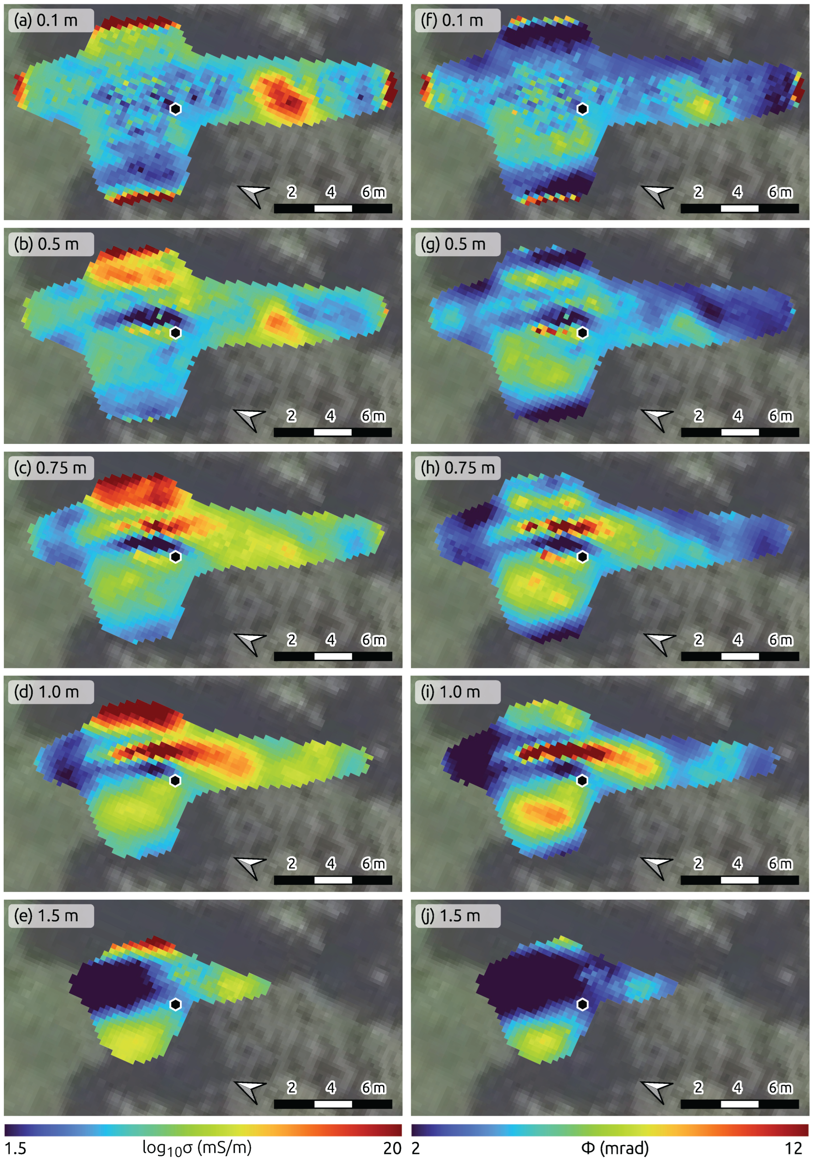
3.2. Detailed Investigation (DI) in the Vicinity of the Documented Grave

The detailed investigation focuses on the area around the grave, using an electrode spacing of 0.25 m adjusted for the expected dimensions of the documented grave. This survey design limits the depth of investigation to approximately 1 m, yet increases both the vertical and horizontal spatial resolution. The sensitivity decreases significantly below this depth due to the short profile lengths (Figure 7).

At shallow depths (0.1 m; Figure 7a,f), both the electrical conductivity (1 to 10 mS/m) and the polarization effect (2 to 8 mrad) reveal a heterogeneous composition of materials. At 0.5 m depth, a distinct low-conductivity anomaly (<2 mS/m) is resolved directly adjacent to the tombstone. Despite its spatial proximity to the documented grave, this anomaly exhibits a negligible polarization effect ($\varphi \le 2$ mrad), which is characteristic of inorganic materials (e.g., [71]). While the position of the anomaly might initially suggest a connection to the grave, the absence of a polarization response—a key indicator of organic matter—clearly shows that it is not associated with the documented grave contents, i.e., wooden boxes containing mortal remains.

With increasing depth, our results reveal a conductive (>18 mS/m) and polarizable (>12 mrad) anomaly directly next to the low-conductivity feature that becomes dominant in the depth slices at 0.75 and 1.0 m (Figure 7c,d,h,i). This anomaly is spatially aligned with the expected location of the grave and exhibits an increase in both conductivity and polarization, as expected due to the accumulation of organic matter (see [55,56,72]). While the electrical conductivity shows diffuse boundaries, the polarization effect delineates a well-defined, rectangular structure, reinforcing the interpretation of a burial. This difference has been addressed in previous studies, where polarization anomalies are attributed to organic carbon bound to grain surfaces, resulting in localized high polarization effects, while elevated electrical conductivity values reflect the accumulation and migration of dissolved organic matter in the pore water (e.g., [55,73]). Despite reduced sensitivity at depths >1 m, we include depth slices at 1.5 m (Figure 7e,j) for completeness. These slices indicate that the anomaly does not extend deeper than 1 m, as the subsurface beyond this depth is dominated by resistive ($\sigma \le 1.5$ mS/m) and non-polarizable ($\varphi \le 2$ mrad) materials, consistent with the natural geology of the area.

4. Discussion

The large-scale investigation reveals a pattern of conductive anomalies with irregular yet geometrically aligned spatial distributions (Figure 6b–e). These anomalies are inconsistent with human-made structures typically associated with cemetery maintenance and instead suggest a natural origin. This observation is supported by the fact that the shapes of these subsurface anomalies differ from the grid-like geometry of grave distribution observed in the intact sections of the cemetery. Consequently, our survey does not indicate the presence of a larger, structured arrangement of graves, such as contiguous rows. However, the known grave remains unresolved in the large-scale dataset, which we attribute to its small dimensions compared to the 1 m electrode spacing used in the data collection.

The inability to resolve the known grave in the large-scale dataset highlights the limitations of low-resolution surveys for detecting small burial features. Our imaging results illustrate that the detection capability of induced polarization imaging is highly dependent on survey geometry and acquisition parameters—particularly electrode spacing and data density—relative to the dimensions and burial depth of the target. In this study, the large-scale survey was intentionally designed with wider electrode spacing to allow for an efficient coverage of the unused section of the cemetery, where no historical cadastre data were available. While this approach supports reconnaissance-scale mapping and the identification of broader anomalies, it lacks the spatial resolution required to detect small graves at shallow depths. In contrast, the detailed investigation was specifically tailored to the expected burial dimensions, based on photographic documentation of the grave, allowing us to resolve a well-defined anomaly at the known location. The use of a 0.25 m electrode spacing provided enhanced spatial resolution within the upper 1.0 m of the subsurface. This finer spacing resulted in a higher density of measurement points across the burial, enabling clear delineation of its boundaries and identification of internal heterogeneities linked to decomposition products. The results demonstrate that high-resolution IP imaging with appropriately chosen electrode spacing is critical for accurate grave characterization. The comparison of both datasets enables a direct assessment of how survey design influences detection capability. These findings underscore the importance of prior knowledge in guiding survey design and parameterization. In contexts where such information is absent, a multi-scale approach—as implemented here—is essential to ensure sufficient sensitivity and spatial resolution for reliably detecting and characterizing unmarked or clandestine graves.

The detailed investigation (Figure 7) resolves a distinct anomaly in the immediate vicinity of the tombstone. For the interpretation of the observed subsurface patterns, we focus on the electrical conductivity at a 1.0 m depth (Figure 8a) and the polarization response at 0.75 m depth (Figure 8b). The electrical conductivity distribution reveals a plume-shaped anomaly emerging from the grave location, likely caused by conductive fluid migrating through preferential flow paths or drainage influenced by topography. Figure 8a includes isolines extracted from the large-scale conductivity model (cf. Figure 6), illustrating that the anomaly is captured, although with reduced spatial detail, even in the LI dataset. This consistency indicates that the anomaly is not an inversion artifact, which reinforces the validity of our interpretation. In the polarization response, elevated values are observed in the area corresponding to the documented grave, as identified from photographic evidence. Compared to the resolved conductivity distribution, the polarization anomaly is more spatially constrained and localized, aligning more closely with the probable extent of the grave. This suggests that the polarization effect may offer a more targeted indicator of the burial location than conductivity alone.

To enhance the interpretation of these observed features, we bin both electrical conductivity (Figure 8b) and polarization response (Figure 8d), and apply a diverging colormap, emphasizing contrasts in the resolved models. For the electrical conductivity, this representation shows high conductivity values (>12 mS/m) over the grave itself, while the plume-shaped anomaly is characterized by intermediate values (8–12 mS/m). In the case of the polarization response, the binned visualization further highlights a well-defined, north–south-oriented anomaly with phase shifts exceeding 10 mrad. We interpret the strong polarization response as indicative of organic carbon adsorbed to mineral grain surfaces within the soil matrix. Based on photographic documentation of the grave contents, we suggest that the source of the elevated organic carbon is the wooden boxes containing the mortal remains. The anomaly forms an almost rectangular pattern, with spatial extent and orientation closely matching the open grave visible in the composite image (Figure 2), reinforcing the interpretation of a localized subsurface feature consistent with the documented burial.

In particular, the decomposition process results in the enrichment of organic matter that is adsorbed to grain surfaces as soil organic carbon, enhancing surface charge and surface area—two key factors governing the strength of the polarization response (i.e., the imaginary component of the complex conductivity). A portion of this organic matter dissolves in pore water and migrates with infiltration, leading to a plume-like anomaly in electrical conductivity at 1.0 m depth (Figure 8a,b). While our interpretation is qualitative and based on contrasts in observed IP responses, we acknowledge that additional parameters—such as clay content and type, ionic strength of pore fluids, and mineralogical composition—may affect both conductivity and polarization responses. However, the influence of these parameters on field-scale IP signatures remains an open question and is still under active discussion in the scientific community (e.g., [74,75]). Although these factors should be considered in future work, particularly in the context of quantitative interpretations, they are not explicitly addressed in our analysis due to the lack of site-specific data. Nonetheless, our study underscores the diagnostic value of induced polarization imaging in detecting chemically altered burial zones, even amid environmental variability.

The depth slices presented in Figure 8 highlight that relying solely on electrical conductivity would not allow for a precise delineation of the grave. While elevated conductivity values are observed in the burial area, the leakage of decomposition fluids reduces the conductivity contrast between the grave and its surroundings. In contrast, the polarization response provides a sharper delineation of the grave relative to adjacent natural materials, a phenomenon that has also been reported in other studies (e.g., [55,56,71,73]). Our final interpretation of the grave location and orientation, as well as the associated plume of groundwater enriched with organic matter, is summarized in Figure 8e. The geometrical agreement with the composite image of the open grave (Figure 2) supports our interpretation and demonstrates the enhanced capability of IP imaging to accurately localize and characterize unmarked graves and associated degradation processes.

5. Conclusions

Our study demonstrates the potential of the induced polarization (IP) method, a geophysical technique, for the non-invasive localization and characterization of unmarked graves in archaeological and forensic contexts. In particular, we introduce an approach utilizing textile electrodes, which enables IP investigations in sensitive areas such as cemeteries or potential crime scenes without disturbing the site. This highlights IP as a powerful remote sensing tool in contexts where invasive methods are legally, culturally, or ethically constrained. The results emphasize the critical role of survey design, with electrode spacing—determining the spatial resolution—being a key factor controlling the resolution of the 3D imaging results.

The study identified a distinct low-conductivity anomaly adjacent to the grave at 0.5 m depth, as well as a conductive, polarizable anomaly at depths between 0.75 and 1.0 m, associated with the grave. This anomaly was characterized by phase shifts greater than 12 mrad, indicating the presence of increased organic carbon, likely from the wooden boxes containing mortal remains. Additionally, the electrical conductivity model revealed a plume-shaped anomaly at 1.0 m depth, which we interpreted as organic matter dissolved in the pore water moving due to gravity forces. The detailed investigation showed that while electrical conductivity alone provided a diffuse boundary for the grave, the polarization imaging allowed for a sharper delineation of the grave and surrounding materials. These findings underline the ability of IP imaging to precisely locate and characterize burial sites, with the polarization response being sensitive to the accumulation of organic carbon in the soil and thus an enhanced interpretation. The study also highlights the importance of spatial resolution and careful survey design for accurate grave detection, as well as the added value of conducting IP measurements instead of ERT surveys.

Future research should aim to refine and expand the application of IP imaging in both methodological and interdisciplinary dimensions. This includes improving detection techniques through controlled studies at dedicated crime scene facilities, implementing fully three-dimensional acquisition geometries for enhanced imaging accuracy, and deepening our understanding of the electrical and polarization responses associated with decomposing organic matter.

Equally important is the optimization of field procedures to increase survey efficiency, enabling the coverage of larger areas within practical timeframes. This is particularly crucial for the operational deployment of IP in forensic and archaeological contexts, where established methods such as ground-penetrating radar and magnetic gradiometry are favored not only for their rapid data acquisition capabilities, but also for their ability to deliver reliable high-resolution subsurface information that supports archaeological interpretation. Beyond this, integrating IP with complementary geophysical techniques through joint application and, more importantly, joint inversion offers considerable potential for enhancing subsurface interpretation in complex burial scenarios. Advances in data fusion methods, including AI-assisted approaches, may further improve detection reliability and reduce ambiguity in grave localization.

Furthermore, future research should test the robustness and applicability of the presented approach across a wider range of geomorphological settings and burial environments. This includes archaeological cemeteries that predate the 20th century, which often exhibit different preservation conditions, burial customs, and levels of organic decomposition. Field validation in such diverse contexts is essential to assess the transferability and reliability of induced polarization imaging in complex burial scenarios. Additionally, comparative studies involving alternative or complementary methods—such as aerial or terrestrial thermal imaging—would provide valuable insights into the relative strengths and limitations of the IP approach, especially under varying environmental and seasonal conditions.

From a broader perspective, successfully translating these techniques into operational forensic and archaeological protocols necessitates close collaboration across geophysics, forensic science, anthropology, and legal disciplines, with careful attention to ethical and cultural sensitivities. The ability of IP imaging to reveal grave-related features non-invasively—particularly in cases where other geophysical methods fail—makes it a valuable complement to traditional archaeogeophysical methods. Building on this interdisciplinary foundation, the methodological advances demonstrated here also offer promising potential for applications beyond forensic and archaeological contexts, such as humanitarian investigations involving unmarked or mass graves, environmental monitoring, and ecological research.

References

1. Ralph, J.; Smith, C.; Jackson, G.; Pamkal, I.B.; Willika, J.; Rubio Perez, R.; Brown, N.; Rankin, G.; Kanungo, A.K.; Choksi, N.; et al. Recording unmarked graves in a remote Aboriginal community: The challenge of cultural heritage driving sustainable development. Archaeologies 2021, 17, 53–78. [Google Scholar] [CrossRef]
2. Reinhartz, D. Unmarked graves: The destruction of the Yugoslav Roma in the Balkan Holocaust, 1941–1945. J. Genocide Res. 1999, 1, 81–89. [Google Scholar] [CrossRef]
3. Różycki, S.; Zapłata, R.; Karczewski, J.; Ossowski, A.; Tomczyk, J. Integrated archaeological research: Archival resources, surveys, geophysical prospection and excavation approach at an execution and burial site: The german nazi labour camp in Treblinka. Geosciences 2020, 10, 336. [Google Scholar] [CrossRef]
4. Thorne, N.; Moss, M. Unmarked Graves: Yet another Legacy of Canada’s Residential School System: An Interview with Niki Thorne. New Am. Stud. J. Forum 2022, 72. [Google Scholar] [CrossRef]
5. Robertshaw, A.S. Killing Them Twice: Ethical Challenges in the Analysis of Human Remains from the Two World Wars. In Ethical Approaches to Human Remains: A Global Challenge in Bioarchaeology and Forensic Anthropology; Squires, K., Errickson, D., Márquez-Grant, N., Eds.; Springer International Publishing: Cham, Switzerland, 2019; pp. 541–556. [Google Scholar] [CrossRef]
6. Pringle, J.; Wisniewski, K.; Ruffell, A.; Hobson, L. Geoforensic search on land. Geol. Today 2024, 40, 146–152. [Google Scholar] [CrossRef]
7. Vinci, G.; Vanzani, F.; Fontana, A.; Campana, S. LiDAR applications in archaeology: A systematic review. Archaeol. Prospect. 2025, 32, 81–101. [Google Scholar] [CrossRef]
8. Adamopoulos, E.; Rinaudo, F. UAS-Based Archaeological Remote Sensing: Review, Meta-Analysis and State-of-the-Art. Drones 2020, 4, 46. [Google Scholar] [CrossRef]
9. Martín Molina, C.; Wisniewski, K.D.; Salamanca, A.; Saumett, M.; Rojas, C.; Gómez, H.; Baena, A.; Pringle, J.K. Monitoring of simulated clandestine graves of victims using UAVs, GPR, electrical tomography and conductivity over 4–8 years post-burial to aid forensic search investigators in Colombia, South America. Forensic Sci. Int. 2024, 355, 111919. [Google Scholar] [CrossRef]
10. Alawadhi, A.; Eliopoulos, C.; Bezombes, F. The detection of clandestine graves in an arid environment using thermal imaging deployed from an unmanned aerial vehicle. J. Forensic Sci. 2023, 68, 1286–1291. [Google Scholar] [CrossRef]
11. Gaffney, C. Detecting trends in the prediction of the buried past: A review of geophysical techniques in archaeology. Archaeometry 2008, 50, 313–336. [Google Scholar] [CrossRef]
12. Horsley, T.J. The use of geophysical survey in archaeology. In Emerging Trends in the Social and Behavioral Sciences: An Interdisciplinary, Searchable, and Linkable Resource; Scott, R.A., Kosslyn, S.M., Eds.; Wiley: Hoboken, NJ, USA, 2015; Volume 1002, p. 18900. [Google Scholar] [CrossRef]
13. Bevan, B.W. Geophysical Exploration for Archaeology: An Introduction to Geophysical Exploration; United States Department of the Interior National Park Service Midwest Archeological Center: Lincoln, NE, USA, 1998. [Google Scholar]
14. Kvamme, K.L. Magnetometry: Nature’s gift to archaeology. In Remote Sensing in Archaeology: An Explicitly North American Perspective; The University of Alabama Press: Tuscaloosa, AB, USA, 2006; pp. 205–233. [Google Scholar]
15. Christiansen, A.V.; Pedersen, J.B.; Auken, E.; Søe, N.E.; Holst, M.K.; Kristiansen, S.M. Improved Geoarchaeological Mapping with Electromagnetic Induction Instruments from Dedicated Processing and Inversion. Remote Sens. 2016, 8, 1022. [Google Scholar] [CrossRef]
16. Callegary, J.B.; Ferré, T.P.A.; Groom, R.W. Vertical Spatial Sensitivity and Exploration Depth of Low-Induction-Number Electromagnetic-Induction InstrumentsAny use of trade, product, or firm names in this publication is for descriptive purposes only and does not imply endorsement by the U.S. government. Vadose Zone J. 2007, 6, 158–167. [Google Scholar] [CrossRef]
17. Barone, P.M.; Di Maggio, R.M. Forensic Geophysics: Ground Penetrating Radar (GPR) Techniques and Missing Persons Investigations. Forensic Sci. Res. 2019, 4, 337–340. [Google Scholar] [CrossRef]
18. Bevan, B.W. The search for graves. Geophysics 1991, 56, 1310–1319. [Google Scholar] [CrossRef]
19. Billinger, M.S. Utilizing Ground Penetrating Radar for the Location of a Potential Human Burial under Concrete. Can. Soc. Forensic Sci. J. 2009, 42, 200–209. [Google Scholar] [CrossRef]
20. Cavalcanti, M.M.; Rocha, M.P.; Blum, M.L.B.; Borges, W.R. The forensic geophysical controlled research site of the University of Brasilia, Brazil: Results from methods GPR and electrical resistivity tomography. Forensic Sci. Int. 2018, 293, 101.e1–101.e21. [Google Scholar] [CrossRef]
21. Doolittle, J.A.; Bellantoni, N.F. The search for graves with ground-penetrating radar in Connecticut. J. Archaeol. Sci. 2010, 37, 941–949. [Google Scholar] [CrossRef]
22. Fiedler, S.; Illich, B.; Berger, J.; Graw, M. The effectiveness of ground-penetrating radar surveys in the location of unmarked burial sites in modern cemeteries. J. Appl. Geophys. 2009, 68, 380–385. [Google Scholar] [CrossRef]
23. Malloch, H.; Shepherd, S.L.; Wolf, L.; Buchanan, M. Ground-penetrating radar (GPR) survey and spatial analysis of the George and Addie Giddens Cemetery, Opelika, Alabama. Southeast. Archaeol. 2024, 43, 1–12. [Google Scholar] [CrossRef]
24. Novo, A.; Lorenzo, H.; Rial, F.I.; Solla, M. 3D GPR in forensics: Finding a clandestine grave in a mountainous environment. Forensic Sci. Int. 2011, 204, 134–138. [Google Scholar] [CrossRef] [PubMed]
25. Pringle, J.K.; Binley, A.; Wisniewski, K.D.; Davenward, B.; Heaton, V.G.; Handley, G.E. Cold case report: Geoforensic brownfield site search for murder victim based on prison informant lead. Forensic Sci. Int. Rep. 2025, 11, 100404. [Google Scholar] [CrossRef]
26. Trinks, I.; Neubauer, W.; Hinterleitner, A. First high-resolution GPR and magnetic archaeological prospection at the Viking Age settlement of Birka in Sweden. Archaeol. Prospect. 2014, 21, 185–199. [Google Scholar] [CrossRef]
27. Trinks, I.; Hinterleitner, A.; Neubauer, W.; Nau, E.; Löcker, K.; Wallner, M.; Gabler, M.; Filzwieser, R.; Wilding, J.; Schiel, H.; et al. Large-area high-resolution ground-penetrating radar measurements for archaeological prospection. Archaeol. Prospect. 2018, 25, 171–195. [Google Scholar] [CrossRef]
28. Everett, M.E. Near-Surface Applied Geophysics; Cambridge University Press: Cambridge, UK, 2013. [Google Scholar]
29. Moser, C.; Binley, A.; Orozco, A.F. 3D electrode configurations for spectral induced polarization surveys of landfills. Waste Manag. 2023, 169, 208–222. [Google Scholar] [CrossRef]
30. Funk, B.; Flores-Orozco, A.; Steiner, M. Possibilities and limitations of cave detection with ERT. Geomorphology 2024, 462, 109332. [Google Scholar] [CrossRef]
31. Ellwood, B.B. Electrical resistivity surveys in two historical cemeteries in northeast Texas: A method for delineating unidentified burial shafts. Hist. Archaeol. 1990, 24, 91–98. [Google Scholar] [CrossRef]
32. Matias, M.S.; da Silva, M.M.; Goncalves, L.; Peralta, C.; Grangeia, C.; Martinho, E. An investigation into the use of geophysical methods in the study of aquifer contamination by graveyards. Surf. Geophys. 2004, 2, 131–136. [Google Scholar] [CrossRef]
33. Berezowski, V.; Mallett, X.; Simyrdanis, K.; Kowlessar, J.; Bailey, M.; Moffat, I. Ground penetrating radar and electrical resistivity tomography surveys with a subsequent intrusive investigation in search for the missing Beaumont children in Adelaide, South Australia. Forensic Sci. Int. 2024, 357, 111996. [Google Scholar] [CrossRef]
34. Pringle, J.K.; Jervis, J.R. Electrical resistivity survey to search for a recent clandestine burial of a homicide victim, UK. Forensic Sci. Int. 2010, 202, e1–e7. [Google Scholar] [CrossRef] [PubMed]
35. Martín Molina, C.; Wisniewski, K.; Heaton, V.; Pringle, J.K.; Avila, E.F.; Herrera, L.A.; Guerrero, J.; Saumett, M.; Echeverry, R.; Duarte, M.; et al. Monitoring of simulated clandestine graves of dismembered victims using UAVs, electrical tomography, and GPR over one year to aid investigations of human rights violations in Colombia, South America. J. Forensic Sci. 2022, 67, 1060–1071. [Google Scholar] [CrossRef]
36. McClymont, A.F.; Bauman, P.D.; Freund, R.A.; Seligman, J.; Jol, H.M.; Reeder, P.; Bensimon, K.; Vengalis, R. Preserving Holocaust history: Geophysical investigations at the Ponary (Paneriai) extermination site. Geophysics 2022, 87, WA15–WA25. [Google Scholar] [CrossRef]
37. Reeder, P.; Jol, H.; Freund, R.; McClymont, A.; Bauman, P.; Šmigelskas, R. Investigations at the Heereskraftfahrpark (HKP) 562 Forced-Labor Camp in Vilnius, Lithuania. Heritage 2023, 6, 466–482. [Google Scholar] [CrossRef]
38. Rubio-Melendi, D.; Gonzalez-Quirós, A.; Roberts, D.; del Carmen García García, M.; Caunedo Domínguez, A.; Pringle, J.K.; Fernández-Álvarez, J.P. GPR and ERT detection and characterization of a mass burial, Spanish Civil War, Northern Spain. Forensic Sci. Int. 2018, 287, e1–e9. [Google Scholar] [CrossRef]
39. Cristino, K.; Doro, K.O.; Armstrong, A.; Forbes, S.; Ribéreau-Gayon, A.; Bank, C.G. Electrical resistivity tomography of simulated graves with buried human and pig remains. Forensic Sci. Int. 2024, 364, 112248. [Google Scholar] [CrossRef]
40. Doro, K.O.; Kolapkar, A.M.; Bank, C.G.; Wescott, D.J.; Mickleburgh, H.L. Geophysical imaging of buried human remains in simulated mass and single graves: Experiment design and results from pre-burial to six months after burial. Forensic Sci. Int. 2022, 335, 111289. [Google Scholar] [CrossRef] [PubMed]
41. Juerges, A.; Pringle, J.K.; Jervis, J.R.; Masters, P. Comparisons of magnetic and electrical resistivity surveys over simulated clandestine graves in contrasting burial environments. Surf. Geophys. 2010, 8, 529–539. [Google Scholar] [CrossRef]
42. Pringle, J.K.; Jervis, J.; Cassella, J.P.; Cassidy, N.J. Time-lapse geophysical investigations over a simulated urban clandestine grave. J. Forensic Sci. 2008, 53, 1405–1416. [Google Scholar] [CrossRef] [PubMed]
43. Jervis, J.R.; Pringle, J.K.; Cassella, J.P.; Tuckwell, G. Using Soil and Groundwater Data to Understand Resistivity Surveys over a Simulated Clandestine Grave. In Criminal and Environmental Soil Forensics; Ritz, K., Dawson, L., Miller, D., Eds.; Springer: Dordrecht, The Netherlands, 2009; pp. 271–284. [Google Scholar] [CrossRef]
44. Pringle, J.K.; Jervis, J.R.; Hansen, J.D.; Jones, G.M.; Cassidy, N.J.; Cassella, J.P. Geophysical monitoring of simulated clandestine graves using electrical and ground-penetrating radar methods: 0–3 years after burial. J. Forensic Sci. 2012, 57, 1467–1486. [Google Scholar] [CrossRef]
45. Pringle, J.K.; Jervis, J.R.; Roberts, D.; Dick, H.C.; Wisniewski, K.D.; Cassidy, N.J.; Cassella, J.P. Long-term geophysical monitoring of simulated clandestine graves using electrical and ground penetrating radar methods: 4–6 years after burial. J. Forensic Sci. 2016, 61, 309–321. [Google Scholar] [CrossRef] [PubMed]
46. Pringle, J.K.; Stimpson, I.G.; Wisniewski, K.D.; Heaton, V.; Davenward, B.; Mirosch, N.; Spencer, F.; Jervis, J.R. Geophysical monitoring of simulated homicide burials for forensic investigations. Sci. Rep. 2020, 10, 7544. [Google Scholar] [CrossRef]
47. Pringle, J.K.; Cassella, J.P.; Jervis, J.R. Preliminary soilwater conductivity analysis to date clandestine burials of homicide victims. Forensic Sci. Int. 2010, 198, 126–133. [Google Scholar] [CrossRef]
48. Pringle, J.K.; Cassella, J.P.; Jervis, J.R.; Williams, A.; Cross, P.; Cassidy, N.J. Soilwater conductivity analysis to date and locate clandestine graves of homicide victims. J. Forensic Sci. 2015, 60, 1052–1060. [Google Scholar] [CrossRef] [PubMed]
49. Barone, P.M.; Matsentidi, D.; Mollard, A.; Kulengowska, N.; Mistry, M. Mapping Decomposition: A Preliminary Study of Non-Destructive Detection of Simulated body Fluids in the Shallow Subsurface. Forensic Sci. 2022, 2, 620–634. [Google Scholar] [CrossRef]
50. Pringle, J.; Ruffell, A.; Jervis, J.; Donnelly, L.; McKinley, J.; Hansen, J.; Morgan, R.; Pirrie, D.; Harrison, M. The use of geoscience methods for terrestrial forensic searches. Earth-Sci. Rev. 2012, 114, 108–123. [Google Scholar] [CrossRef]
51. Flores Orozco, A.; Steiner, M.; Katona, T.; Roser, N.; Moser, C.; Stumvoll, M.J.; Glade, T. Application of induced polarization imaging across different scales to understand surface and groundwater flow at the Hofermuehle landslide. CATENA 2022, 219, 106612. [Google Scholar] [CrossRef]
52. Binley, A.; Slater, L. Resistivity and Induced Polarization: Theory and Applications to the Near-Surface Earth; Cambridge University Press: Cambridge, UK, 2020. [Google Scholar] [CrossRef]
53. Lesmes, D.P.; Friedman, S.P. Relationships between the electrical and hydrogeological properties of rocks and soils. In Hydrogeophysics; Springer: Berlin/Heidelberg, Germany, 2005; pp. 87–128. [Google Scholar] [CrossRef]
54. Slater, L.; Glaser, D. Controls on induced polarization in sandy unconsolidated sediments and application to aquifer characterization. Geophysics 2003, 68, 1547–1558. [Google Scholar] [CrossRef]
55. Flores Orozco, A.; Gallistl, J.; Steiner, M.; Brandstätter, C.; Fellner, J. Mapping biogeochemically active zones in landfills with induced polarization imaging: The Heferlbach landfill. Waste Manag. 2020, 107, 121–132. [Google Scholar] [CrossRef]
56. Katona, T.; Gilfedder, B.S.; Frei, S.; Bücker, M.; Flores Orozco, A. High-resolution induced polarization imaging of biogeochemical carbon-turnover hot spots in a peatland. Biogeosci. Discuss. 2021, 18, 4039–4058. [Google Scholar] [CrossRef]
57. Elis, V.R.; Almeida, E.R.; Porsani, J.L.; Stangari, M.C. Ground-penetrating radar, resistivity, and induced polarization applied in forensic research in tropical soils. In Proceedings of the 18th International Conference on Ground Penetrating Radar, Golden, CO, USA, 14–19 June 2020; Society of Exploration Geophysicists: Houston, TX, USA, 2020; pp. 224–227. [Google Scholar] [CrossRef]
58. Buckel, J.; Mudler, J.; Gardeweg, R.; Hauck, C.; Hilbich, C.; Frauenfelder, R.; Kneisel, C.; Buchelt, S.; Blöthe, J.H.; Hördt, A.; et al. Identifying mountain permafrost degradation by repeating historical electrical resistivity tomography (ERT) measurements. Cryosphere 2023, 17, 2919–2940. [Google Scholar] [CrossRef]
59. Buckel, J.; Matthias, B.; Hördt, A.; Mudler, J. Elektrode mit leitfähigem Textilmaterial zur Elektrischen Widerstandsmessung des. Untergrundes. Patent DE102021110721, 6 June 2025. [Google Scholar]
60. Bast, A.; Pavoni, M.; Lichtenegger, M.; Buckel, J.; Boaga, J. The Use of Textile Electrodes for Electrical Resistivity Tomography in Periglacial, Coarse Blocky Terrain: A Comparison With Conventional Steel Electrodes. Permafr. Periglac. Process. 2025, 36, 110–122. [Google Scholar] [CrossRef]
61. Flores Orozco, A.; Aigner, L.; Gallistl, J. Investigation of cable effects in spectral induced polarization imaging at the field scale using multicore and coaxial cables. Geophysics 2021, 86, E59–E75. [Google Scholar] [CrossRef]
62. Flores Orozco, A.; Gallistl, J.; Bücker, M.; Williams, K.H. Decay curve analysis for data error quantification in time-domain induced polarization imaging. Geophysics 2018, 83, E75–E86. [Google Scholar] [CrossRef]
63. Riley, S.J.; DeGloria, S.D.; Elliot, R. Index that quantifies topographic heterogeneity. Intermt. J. Sci. 1999, 5, 23–27. [Google Scholar]
64. Martin, T.; Günther, T.; Orozco, A.F.; Dahlin, T. Evaluation of spectral induced polarization field measurements in time and frequency domain. J. Appl. Geophys. 2020, 180, 104141. [Google Scholar] [CrossRef]
65. Flores Orozco, A.; Kemna, A.; Zimmermann, E. Data error quantification in spectral induced polarization imaging. Geophysics 2012, 77, E227–E237. [Google Scholar] [CrossRef]
66. Günther, T.; Rücker, C.; Spitzer, K. Three-dimensional modelling and inversion of DC resistivity data incorporating topography–II. Inversion. Geophys. J. Int. 2006, 166, 506–517. [Google Scholar] [CrossRef]
67. LaBrecque, D.J.; Miletto, M.; Daily, W.; Ramirez, A.; Owen, E. The effects of noise on Occam’s inversion of resistivity tomography data. Geophysics 1996, 61, 538–548. [Google Scholar] [CrossRef]
68. Günther, T.; Rücker, C. Boundless Electrical Resistivity Tomography BERT 2—The User Tutorial. 2015. Available online: http://www.resistivity.net/download/bert-tutorial.pdf (accessed on 30 July 2025).
69. Rücker, C.; Günther, T.; Wagner, F.M. pyGIMLi: An open-source library for modelling and inversion in geophysics. Comput. Geosci. 2017, 109, 106–123. [Google Scholar] [CrossRef]
70. Oldenburg, D.W.; Li, Y. Inversion of induced polarization data. Geophysics 1994, 59, 1327–1341. [Google Scholar] [CrossRef]
71. Strobel, C.; Dörrich, M.; Stieff, E.H.; Huisman, J.A.; Cirpka, O.A.; Mellage, A. Organic matter matters—The imaginary conductivity of sediments rich in solid organic carbon. Geophys. Res. Lett. 2023, 50, e2023GL104630. [Google Scholar] [CrossRef]
72. McLachlan, P.; Karloukovski, V.; Binley, A. Field-based estimation of cation exchange capacity using induced polarization methods. Earth Surf. Process. Landforms 2024, 49, 4928–4944. [Google Scholar] [CrossRef]
73. Steiner, M.; Katona, T.; Fellner, J.; Flores Orozco, A. Quantitative water content estimation in landfills through joint inversion of seismic refraction and electrical resistivity data considering surface conduction. Waste Manag. 2022, 149, 21–32. [Google Scholar] [CrossRef] [PubMed]
74. Mendieta, A.; Jougnot, D.; Leroy, P.; Maineult, A. Spectral Induced Polarization Characterization of Non-Consolidated Clays for Varying Salinities—An Experimental Study. J. Geophys. Res. Solid Earth 2021, 126, e2020JB021125. [Google Scholar] [CrossRef]
75. Zibulski, E.; Klitzsch, N. Influence of Inner Surface Roughness on the Spectral Induced Polarization Response—A Numerical Study. J. Geophys. Res. Solid Earth 2023, 128, e2022JB025548. [Google Scholar] [CrossRef]
76. Steiner, M.; Flores Orozco, A. 3D Complex Resistivity Survey of a Known Burial Site at an Inactive Cemetery, 2025. Zenodo, 2025; in press. [Google Scholar] [CrossRef]
Figure 1. Measurement setup used in this study, showing the Syscal Pro Switch control unit from IRIS Instruments (Orléans, France), an external battery for current injection, and the electrode cable. Textile electrodes are attached at regular intervals along the cable. The inset provides a close-up of a textile electrode, including its connection to the cable with pegs.
Remotesensing 17 02687 g001
Figure 2. Composite image of a historic funeral photograph superimposed onto a recent image of the same location. This overlay allows for the approximation of the grave’s position within the present-day environment. The recent photograph also shows electrode cables, illustrating that the geophysical measurements of this study were conducted across the location of this known grave.
Remotesensing 17 02687 g002
Figure 3. Maps of the investigation area at different scales. (a) Overview of the cemetery with the hillshade of the 0.25 m DEM and 0.25 m isolines for the large-scale investigation area. (b) Zoom-in of large-scale investigations (LIs) with 1 m electrode spacing, showing the area of detailed investigations. (c) Detailed view of the 0.25 m electrode spacing investigations (DIs). Orange lines indicate profile locations and orientations; white arrows show measurement directions. The hexagon marks the tombstone location. Note: Subplot orientations vary; north is indicated in each panel.
Remotesensing 17 02687 g003
Figure 4. Flowchart illustrating the computation of the S-curve probability for the Topographic Impact Factor (TIF) from a digital elevation model (DEM).
Remotesensing 17 02687 g004
Figure 5. Topographic analysis and its influence on geophysical investigations. (a) Hillshade of the 0.25 m DEM with 0.25 m isolines. (b) Terrain Ruggedness Index (TRI). (c) Gradient magnitude | z | . (d,e) Topographic Impact Factor (TIF) for 0.25 m and 1.0 m electrode spacings. (f,g) Classification of TIF based on the probability of its influence on inversion, for 0.25 m and 1.0 m spacing. Orange lines indicate profile locations and orientations; white arrows show measurement directions. The hexagon marks the tombstone location. Note: Subplot orientations vary; north is indicated in each panel.
Remotesensing 17 02687 g005
Figure 6. Depth slices extracted from 3D models of electrical conductivity (ae) and polarization effect (fj), obtained through inversion of data collected in the open area adjacent to the known grave (1.0 m electrode spacing). Slices are shown for depths of 0.1, 0.5, 0.75, 1.0, and 1.5 m. Areas of low sensitivity are blanked. The hexagon marks the tombstone location. Note: Subplot orientations vary; north is indicated in each panel.
Remotesensing 17 02687 g006
Figure 7. Depth slices extracted from 3D models of electrical conductivity (ae) and polarization effect (fj), obtained through inversion of data collected in the vicinity of the known grave (0.25 m electrode spacing). Slices are shown for depths of 0.1, 0.5, 0.75, 1.0, and 1.5 m. Areas of low sensitivity are blanked. The hexagon marks the tombstone location. Note: Subplot orientations vary; north is indicated in each panel.
Remotesensing 17 02687 g007
Figure 8. Visualization of geophysical results from data collected with 0.25 m electrode spacing, highlighting anomalies linked to the grave and a potential leachate plume. (a,c) Depth slices through 3D models of electrical conductivity (1.0 m depth) and polarization effect (0.75 m depth). (b,d) Classification of conductivity and polarization values into five groups to emphasize spatial patterns; interpreted outlines of the plume and grave are shown as solid polygons. (e) Summary of interpreted grave and plume extents with data collection profiles (0.25 m and 1.0 m spacing). Orange lines indicate profile locations and orientations; the hexagon marks the tombstone location. Note: Subplot orientations vary; north is indicated in each panel.
Remotesensing 17 02687 g008