A Soil Moisture-Informed Seismic Landslide Model Using SMAP Satellite Data

Abstract

Earthquake-triggered landslides pose significant hazards to lives and infrastructure. While existing seismic landslide models primarily focus on seismic and terrain variables, they often overlook the dynamic nature of hydrologic conditions, such as seasonal soil moisture variability. This study addresses this gap by incorporating satellite-based soil moisture data from NASA’s Soil Moisture Active Passive (SMAP) mission into the assessment of seismic landslide occurrence. Using landslide inventories from five major earthquakes (Nepal 2015, New Zealand 2016, Papua New Guinea 2018, Indonesia 2018, and Haiti 2021), a balanced global dataset of landslide and non-landslide cases was compiled. Exploratory analysis revealed a strong association between elevated pre-event soil moisture and increased landslide occurrence, supporting its relevance in seismic slope failure. Moreover, a Random Forest model was trained and tested on the dataset and demonstrated excellent predictive performance. To assess the generalizability of the model, a leave-one-earthquake-out cross-validation approach was also implemented, in which the model trained on four events was tested on the fifth. This approach outperformed comparable models that did not consider soil moisture, such as the United States Geological Survey (USGS) seismic landslide model, confirming the added value of satellite-based soil moisture data in improving seismic landslide susceptibility assessments.

1. Introduction

Landslides stand as some of the most destructive hazards, leading to significant loss of life, widespread infrastructure damage, and lasting societal and environmental repercussions [1,2,3,4,5]. When triggered by earthquakes, their impact intensifies as seismic shaking destabilizes slopes, initiating a cascade of ground failures that amplify destruction [6,7,8]. Earthquake-induced landslides are especially common in mountainous regions, where steep terrain and loose sediments greatly increase vulnerability. These events contribute substantially to the overall damage and losses associated with seismic disasters [9,10,11]. The 2008 Wenchuan earthquake in China triggered over 197,000 landslides, resulting in more than 20,000 fatalities [12,13]. Similarly, the 2015 Gorkha earthquake in Nepal caused nearly 25,000 landslides [14,15,16], isolating communities and disrupting vital services. The 2018 Palu earthquake in Indonesia, which triggered approximately 15,700 co-seismic landslides, led to over 2000 fatalities, displaced over 206,000 individuals, and caused property losses of 911 million US dollars with reconstruction costs projected at 1.5 billion US dollars [17,18,19]. The impacts of seismic landslides extend far beyond immediate casualties. Landslides frequently block transportation routes, sever lifelines, and delay rescue and recovery efforts. Blocked rivers often form landslide dams that can result in catastrophic flooding downstream [20,21]. In the long term, landslides reshape landscapes, accelerate erosion, degrade water quality, and damage agricultural lands, leading to lasting socioeconomic challenges, particularly in resource-constrained regions [22,23]. Given the widespread impact of earthquake-induced landslides, rapid assessment of their distribution and extent following an earthquake is crucial [24,25,26,27,28,29,30,31]. Identifying affected areas enables efficient rescue operations, resource allocation, and mitigation planning. By prioritizing timely analysis and response, the devastating effects of landslides can be mitigated, reducing risks and enhancing resilience in vulnerable communities.

Landslide predictive models encompass a spectrum of methodologies categorized based on their theoretical framework and application scope [25,28]. The primary approaches include mechanistic models, heuristic methods, statistical models, and machine learning (ML) techniques [25,28,32,33], with hybrid approaches emerging as integrative solutions [31,34]. Mechanistic models, based on physical principles like slope stability analysis and Newmark’s sliding block method, are effective for site-specific landslide assessments when detailed geotechnical data are available, making them ideal for infrastructure-focused studies [21,30,31,35,36,37]. Recent advancements, including simplified Newmark methods, have improved their applicability to regional scales by reducing computational demands [38,39,40]. Moreover, innovations like coupling and decoupling analyses have further enhanced the ability of these models to capture dynamic interactions between seismic forces and slope stability [41]. However, assumptions such as rigid sliding directions limit their ability to represent complex, real-world conditions, affecting scalability for large-scale hazard mapping [39].

Heuristic models use expert judgment to assign weights to factors like slope, lithology, and land cover, making them suitable for data-scarce regions and simple to implement using Geographic Information System (GIS) tools [42,43,44,45,46,47]. However, their subjectivity often leads to inconsistencies and limits reproducibility across regions [42,48]. Statistical models have historically formed the foundation of landslide susceptibility mapping by systematically analyzing relationships between landslide occurrences and conditioning factors [32,46,49,50]. Techniques like logistic regression (LR) [27,51,52,53], frequency ratio analysis [54], and weight-of-evidence methods [55] use historical landslide inventories to establish probabilistic frameworks for prediction [56,57]. GIS and remote sensing advances have further improved these models by integrating diverse geospatial and temporal datasets [58,59,60].

Logistic regression is widely used for its simplicity and ability to quantify relationships between variables and landslide probability, bridging statistical and machine learning methods [61,62]. Frequency ratio and weight-of-evidence methods also effectively rank and combine contributing factors, making them suitable for data-limited regions. Recent multivariate and Bayesian approaches have improved accuracy by capturing complex interrelationships [63]. However, these models assume that past patterns persist, which may not hold under changing climate, land use, or seismic conditions [64], and they rely on historical inventories that may introduce spatial and temporal biases [30,56].

The rise in machine learning (ML) has transformed geohazard prediction, including landslide susceptibility modeling. ML algorithms—such as Random Forest (RF), SVM, ANN, GBM, and CNN—can capture complex nonlinear relationships [34,65,66,67,68,69,70,71] without assuming data distributions, making them well-suited for diverse geologic and climatic settings and high-dimensional datasets [72,73]. However, their “black box” nature can hinder interpretability and adoption [34]. Advances in explainable AI, such as SHapley Additive exPlanations (SHAP), are beginning to bridge this gap by identifying key factors driving predictions [61,74]. To address interpretability concerns, hybrid approaches have emerged, integrating physical, statistical, and ML models [30,54,63,69,75,76,77,78,79,80,81,82]. By combining the mechanistic insights of physical models with the predictive power of ML frameworks, these methods balance accuracy and transparency [81,82,83]. For instance, coupling ML with Newmark displacement models [84,85] has enhanced predictive capacity, particularly in data-scarce environments. Hybrid methods also leverage physical constraints to reduce overfitting, a common issue in ML applications, ensuring more generalizable results.

Predicting seismic landslides is inherently challenging due to the intricate interplay of diverse factors that vary spatially and temporally, necessitating the evolution of predictive techniques. The transition from empirical and heuristic methods to advanced machine learning (ML) and hybrid approaches reflects the increasing complexity and availability of data required to address these challenges. While traditional methods continue to serve localized studies, integrating ML and hybrid frameworks offers new avenues for scalable and accurate hazard assessments [86]. Seismic indices, such as ground shaking intensity and proximity to fault lines, serve as primary instigators of slope instability [27,48,87]. However, their impact is modulated by geotechnical and geological properties like soil type, fine content, and relative density [74,88]. Fault zones and the strength of underlying lithology further determine the susceptibility of slopes to failure [89]. Topographical features including slope, elevation, aspect, and topographic wetness index, also play a critical role in channeling and amplifying seismic forces, often dictating the scale and type of landslides triggered [90]. Environmental factors, such as antecedent rainfall, soil moisture, vegetation cover, and proximity to water bodies, introduce additional layers of complexity [91]. For instance, prolonged rainfall can weaken soil cohesion and increase pore-water pressure during earthquakes, reducing slope stability, while vegetation can either stabilize slopes through root reinforcement or increase susceptibility by adding weight. Changes in the water table, driven by seasonal or event-based variations, further affect slope integrity, especially in regions with fluctuating hydrological conditions.

Dynamic interactions among landslide-related factors, such as soil properties, vegetation cover, and hydrological conditions, often evolve over time in response to natural and human-induced changes [92,93]. For example, prolonged rainfall can alter subsurface water distribution, while deforestation and urbanization can disrupt natural drainage and exacerbate instability. These evolving processes highlight the necessity for adaptable models that can account for temporal and spatial variability [94]. Incorporating the dynamic essence of these factors into predictive frameworks is essential for creating models that remain robust across diverse landscapes and changing environmental conditions, ultimately enhancing the accuracy of hazard assessments and disaster mitigation efforts.

Soil moisture plays a pivotal role in landslide susceptibility [28,91,95] by directly influencing soil’s apparent cohesion, pore water pressure, and shear strength [58,87,96]. Elevated soil moisture can contribute to slope instability under seismic loading by increasing pore water pressure and reducing effective stress, particularly in loose or saturated soils. Also, low soil moisture can, under certain conditions, increase apparent soil strength; however, this effect is transient and may obscure latent slope instability, especially if followed by rapid infiltration from rainfall or snowmelt. The dynamic nature of soil moisture—driven by seasonal changes, precipitation patterns, and hydrological processes—makes it a vital parameter for modeling landslide susceptibility [58]. Previous landslide susceptibility models have often relied on indirect proxies for soil moisture, such as average water table depth, historical precipitation data, distance to water bodies, and topographic wetness indices [27,62,89]. While these parameters provide general correlations with soil saturation, they lack the ability to capture dynamic, event-specific soil water content variations and pre-event saturation conditions. This limitation can lead to over- or underestimations in predicting landslide susceptibility for specific events. Recognizing these shortcomings, there is some potential in integrating near-real-time soil moisture datasets, calibrated for surface and root-zone soil moisture conditions [58,59,97]. Such advancements have the potential to improve landslide models.

Remote sensing and satellite data play an increasingly important role in geotechnical earthquake engineering [58], including landslide studies [98,99,100]. Aerial and satellite imagery are widely used for landslide detection [100,101,102] and to generate high-quality inventories [14,17,91,103,104,105], which support post-event analysis and model training. Beyond landslide detection, remote sensing technologies have revolutionized the availability and quality of factors contributing to natural hazards [58], including landslide studies. Satellite data are used to derive global datasets of landslide causative factors, such as slope and vegetation cover, enabling large-scale hazard assessments. However, to the best of our knowledge, the use of satellite-derived soil moisture data specifically for earthquake-induced landslides has not yet been explored. This is despite its demonstrated use in studies of rainfall-triggered landslides, where soil moisture has been used to assess slope stability under varying hydrological conditions [106,107,108,109,110].

The Soil Moisture Active Passive (SMAP) Earth-observing satellite, launched in 2015 by NASA, is a groundbreaking mission designed to monitor soil moisture dynamics globally. SMAP measures the brightness temperature of Earth’s surface using an L-band radiometer, which allows it to estimate soil moisture content in the top 5 cm of the soil column with high accuracy. This data is retrieved at a spatial resolution of 9 km, using the Backus–Gilbert optimal interpolation method, and updated every 2–3 days, providing near-real-time insights into land surface conditions [59,111]. SMAP satellite surpasses its predecessors, such as the Tropical Rainfall Measuring Mission (TRMM) and Advanced Microwave Scanning Radiometer 2 (AMSR-2), by offering significantly finer spatial resolution (9 km) and improved accuracy. SMAP revisits each region globally every 1–3 days, enabling frequent monitoring of surface soil moisture conditions. Comparative studies have shown that SMAP’s soil moisture products outperform other satellite-based datasets, including AMSR-2, SMOS, and simulated datasets like GLDAS and ERA5, by exhibiting higher correlation coefficients and lower unbiased root mean square errors (ubRMSE) [58,112]. These advantages make SMAP a valuable tool for monitoring soil moisture with unprecedented precision and reliability [51,58].

SMAP’s datasets have been validated extensively [113,114] and applied in diverse fields, including weather and climate prediction [115], agricultural monitoring [116], and natural hazard assessments like earthquakes [51,58], floods [117,118], rainfall-induced landslides [119], and sinkhole [120]. Recently, several studies have explored its application in geotechnical earthquake engineering [51,58], shedding light on its potential for advancing understanding and predictive modeling. Farahani and Ghayoomi used SMAP data to develop Soil moisture-based global liquefaction model (SMGLM) [51]. The ability of SMAP to monitor both surface and root-zone soil moisture provides a unique advantage in understanding pre-event and post-event soil moisture conditions, offering potential advancements in landslide susceptibility assessments.

This study aims to employ a data-driven approach to evaluate the impact of integrating soil moisture as a key dynamic variable in landslide susceptibility modeling. Using polygon-mapped landslide inventories from four major earthquakes—Gorkha, Nepal (2015) [14]; Kaikōura, New Zealand (2016) [103]; Papua New Guinea (2018) [91]; Palu, Indonesia (2018) [17]— along with a comprehensive point-based inventory from the Nippes, Haiti (2021) [104], a unified database of landslide and non-landslide occurrence samples is constructed. The study investigates the relationship between SMAP-derived soil moisture data and other causative factors, such as topography and seismic intensity, as well as the interactions among these factors within the context of the landslide database. Random forest algorithm is then applied to this dataset to develop a Soil moisture-informed seismically induced landslide Model. The performance of this model is evaluated and compared with the United States Geological Survey (USGS) seismic landslide model, highlighting the potential of near-real-time soil moisture data to enhance predictive accuracy.

2. Materials and Methods

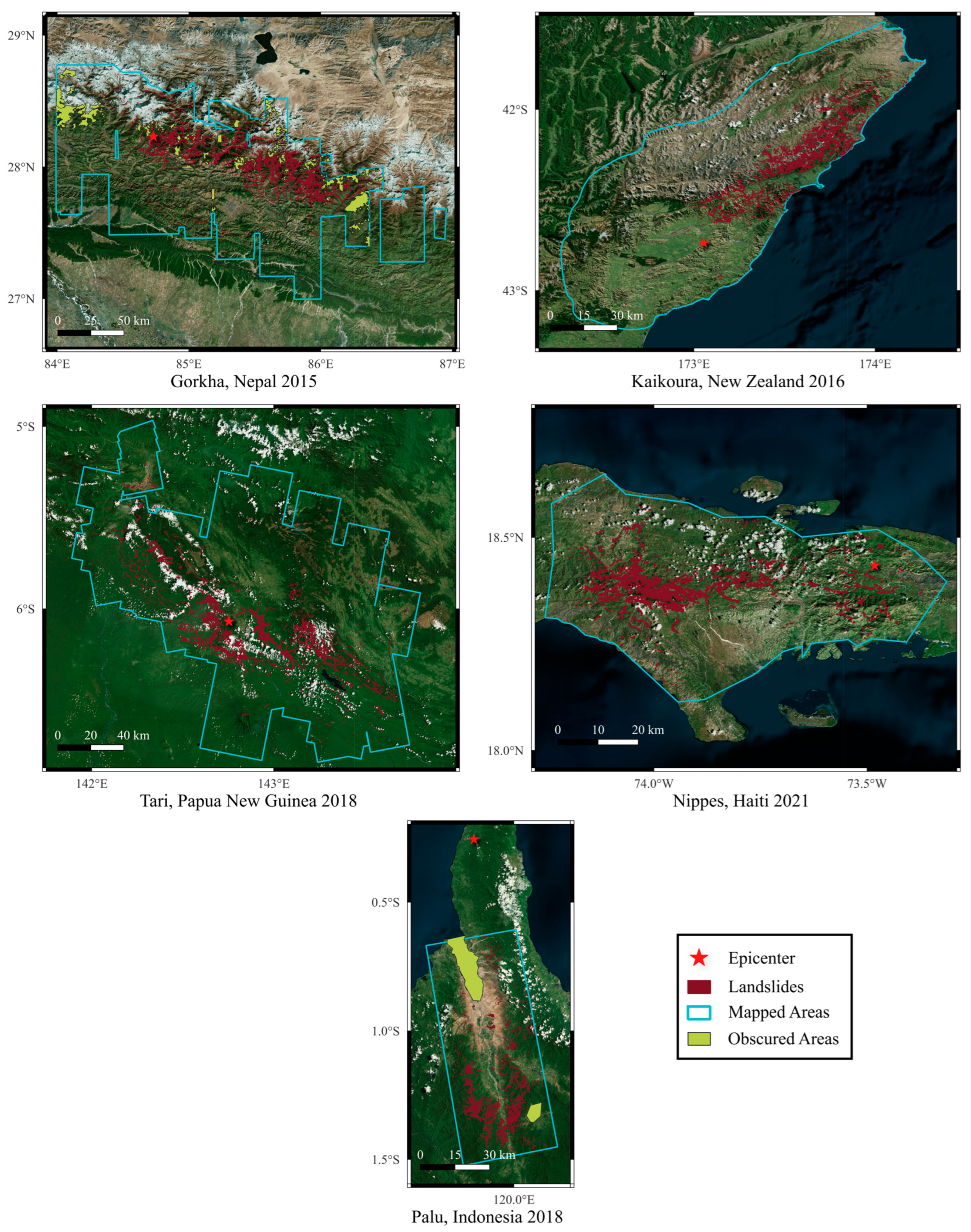
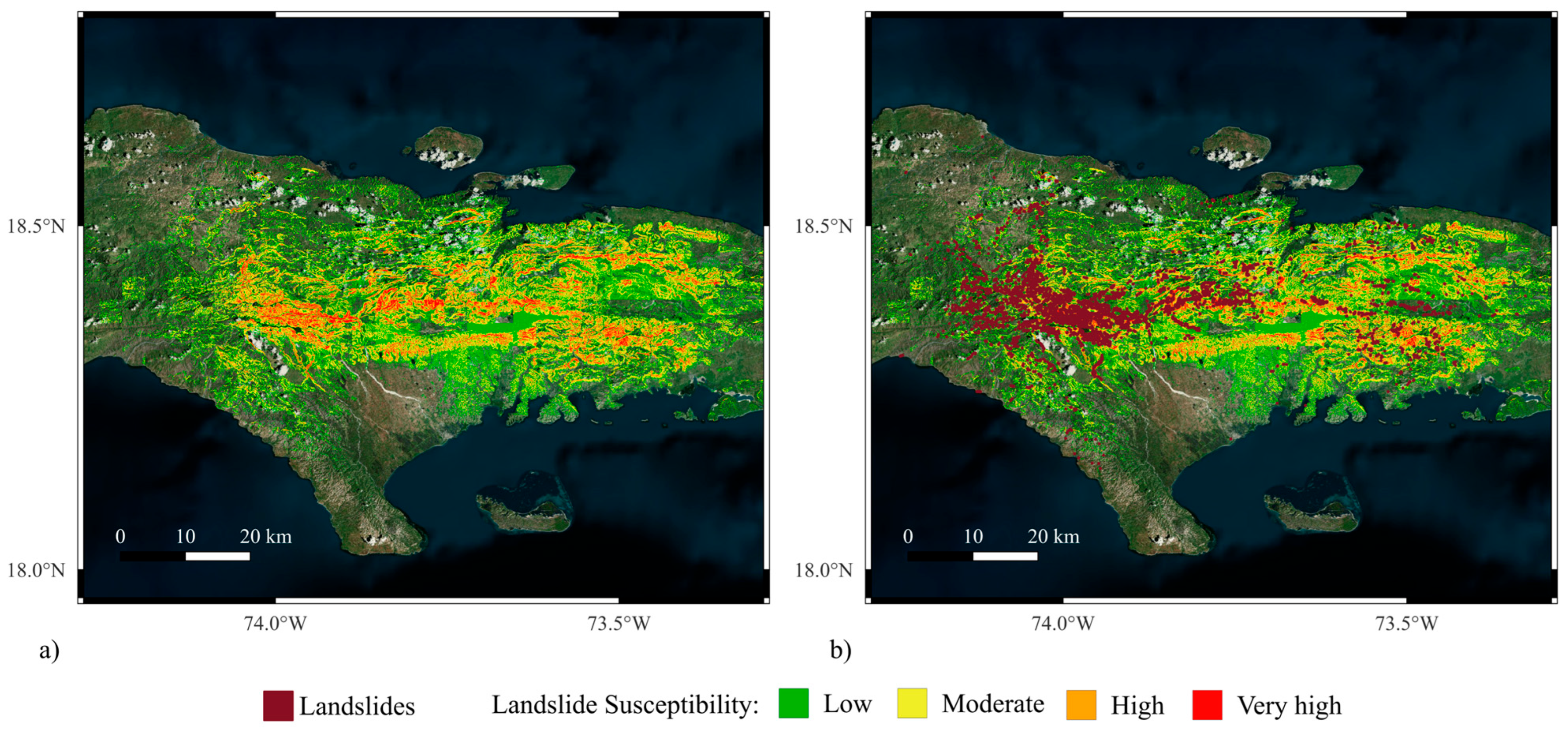
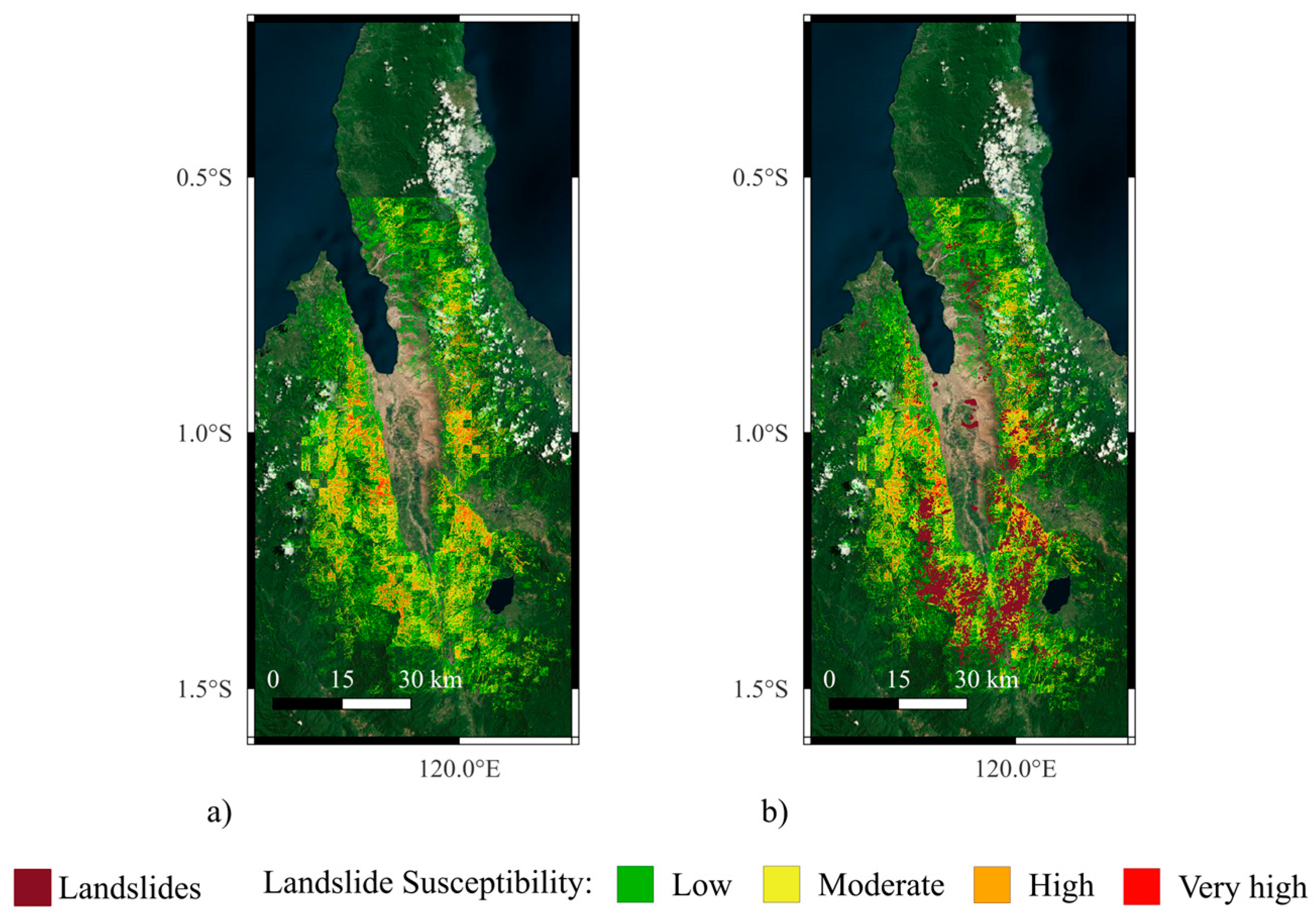
2.1. Landslide Inventories

To identify relevant case studies, moderate to high-intensity earthquakes that occurred between April 2015, and the present were reviewed. This timeframe aligns with the operational period of the Soil Moisture Active Passive (SMAP) satellite. Events were selected based on the availability and completeness of high-quality post-earthquake landslide inventories. Given the coarse spatial resolution of SMAP and rainfall datasets, major earthquakes that impacted broader regions were prioritized over events with smaller affected footprints. The five selected events are briefly described below.

Nepal 2015 (Mw 7.8 Gorkha Earthquake): The 25 April 2015, Gorkha earthquake triggered extensive landslide activity across central Nepal. Over 24,800 landslides were mapped using high-resolution satellite imagery, including WorldView-2/3 and Pleiades, as reported by Roback et al. [14]. The polygon-based inventory delineated both source and deposit zones, with landslides concentrated east of the rupture zone where steep slopes, heavy rainfall, and intense shaking intersected. The Nepal dataset is particularly valuable due to its scale, resolution, and the availability of supporting reconnaissance data.

New Zealand 2016 (Mw 7.8 Kaikōura Earthquake): On 14 November 2016, the Kaikōura earthquake in New Zealand’s South Island triggered more than 10,000 co-seismic landslides across approximately 10,000 km². Massey et al. [103] developed a detailed inventory based on aerial photography and LiDAR, with landslides ranging from small failures to massive slides over 20 million m³. Many large failures occurred near fault ruptured faults. Coastal slopes, especially near uplifted marine terraces, also showed a markedly higher landslide density compared to inland regions. The dataset is among the most comprehensive for a modern seismic landslide event.

Indonesia 2018 (Mw 7.5 Palu Earthquake): The 28 September 2018 Palu earthquake in Sulawesi, Indonesia, was a supershear strike-slip event that triggered over 7063 mapped landslides, as reported by Zhao [17]. Mapping was based on WorldView, Sentinel, and Google Earth imagery, with the total affected area spanning about 30 km². The inventory also includes catastrophic flow slides on gentle slopes in Petobo, Jono Oge, and Sibalaya, where saturated soils and suspected liquefaction effects played a critical role. These conditions highlight the significance of hydrologic factors, such as elevated antecedent soil moisture, in amplifying ground failures in this event.

Papua New Guinea 2018 (Mw 7.5 Papua Highlands Earthquake): On 25 February 2018, an earthquake in the remote Highlands of Papua New Guinea generated over 11,600 mapped landslides. The inventory developed by Tanyaş et al. [91] spans about 145 km², with most failures occurring in steep terrain composed of Darai Limestone and volcaniclastics. Over 10,000 slides were co-seismic, while the rest were triggered by aftershocks and post-seismic rainfall. Despite slightly below-average rainfall, certain areas received more than 80 mm/day. The study [91] reported that 15-day antecedent precipitation exceeding 180 mm significantly increased landslide likelihood, highlighting the importance of soil moisture in seismic landslide susceptibility.

Haiti 2021 (Mw 7.2 Nippes Earthquake): The 14 August 2021, Nippes earthquake in southwestern Haiti triggered 4893 mapped landslides, predominantly in steep terrain along the Enriquillo-Plantain Garden Fault. The inventory, developed by the USGS [104], was derived from Sentinel-2, PlanetScope, and WorldView imagery. Tropical Cyclone Grace passed over the region two days after the earthquake, contributing to substantial rainfall that likely reactivated marginally stable slopes. The combined influence of strong shaking and elevated soil moisture created conditions favorable for cascading geohazards.

The landslide inventories for Nepal [14], Indonesia [17], Papua New Guinea [91], and Haiti [104] are publicly available through the USGS Open Repository of Earthquake-Triggered Ground-Failure Inventories [121]. For the New Zealand earthquake, data published by Massey et al. [103] and Tanyaş et al. [122] were used. Figure 1 illustrates the spatial extent and mapped landslides for each inventory. It is noted that the inventories for Nepal, New Zealand, Indonesia, and Papua New Guinea were polygon-based, while the Haiti dataset was provided in point format.

It should be noted that the landslide inventories used in this study did not label and classify failure types (e.g., shallow, deep-seated, debris flow) [123]. All five earthquake-induced landslide inventories were primarily compiled using remote sensing techniques. While effective for broad mapping, this approach may lack detailed failure-type annotations. Nonetheless, supporting documentation and field reports suggest that the majority of landslides in this study fall within the categories of shallow translational slides and debris flows [124]. For example, the Nepal (2015) inventory by Roback et al. [14] predominantly includes shallow translational slides along with some flow-like runouts. The New Zealand (2016) inventory [103] provides the most detailed failure-type information, identifying mostly shallow slides, as well as some rockfalls and minor debris flows. Landslides in the Indonesia (2018) [17] event are also mainly shallow, with a limited number of large-scale flowslides. In the Haiti (2021) inventory [104], debris slides on steep slopes are most prevalent, with a few occurrences of rockfalls or slumps along road cuts. For Papua New Guinea (2018) [91], debris flows, debris slides, and mudslides were the dominant failure types. These reports indicate that shallow landslides are the prevailing mode of failure across all five events.

Although some landslide susceptibility studies—particularly those focused on small or localized inventories—do incorporate failure-type classifications [31,125,126,127], the vast majority of regional- and global-scale models do not. This is primarily due to the lack of consistent failure-type labeling across large inventories or multi-inventory studies [27,74,89]. Notably, several influential and widely cited seismic landslide models [34,86]—such as those by Nowicki Jessee et al. [27] (used as the USGS baseline model in our study) and He et al. [89] (also used for comparison in this study)—rely on landslide inventories that do not differentiate between failure types. This study shares the same limitation, as it does not distinguish between different landslide types due to the lack of consistent failure-type classification across the inventories.

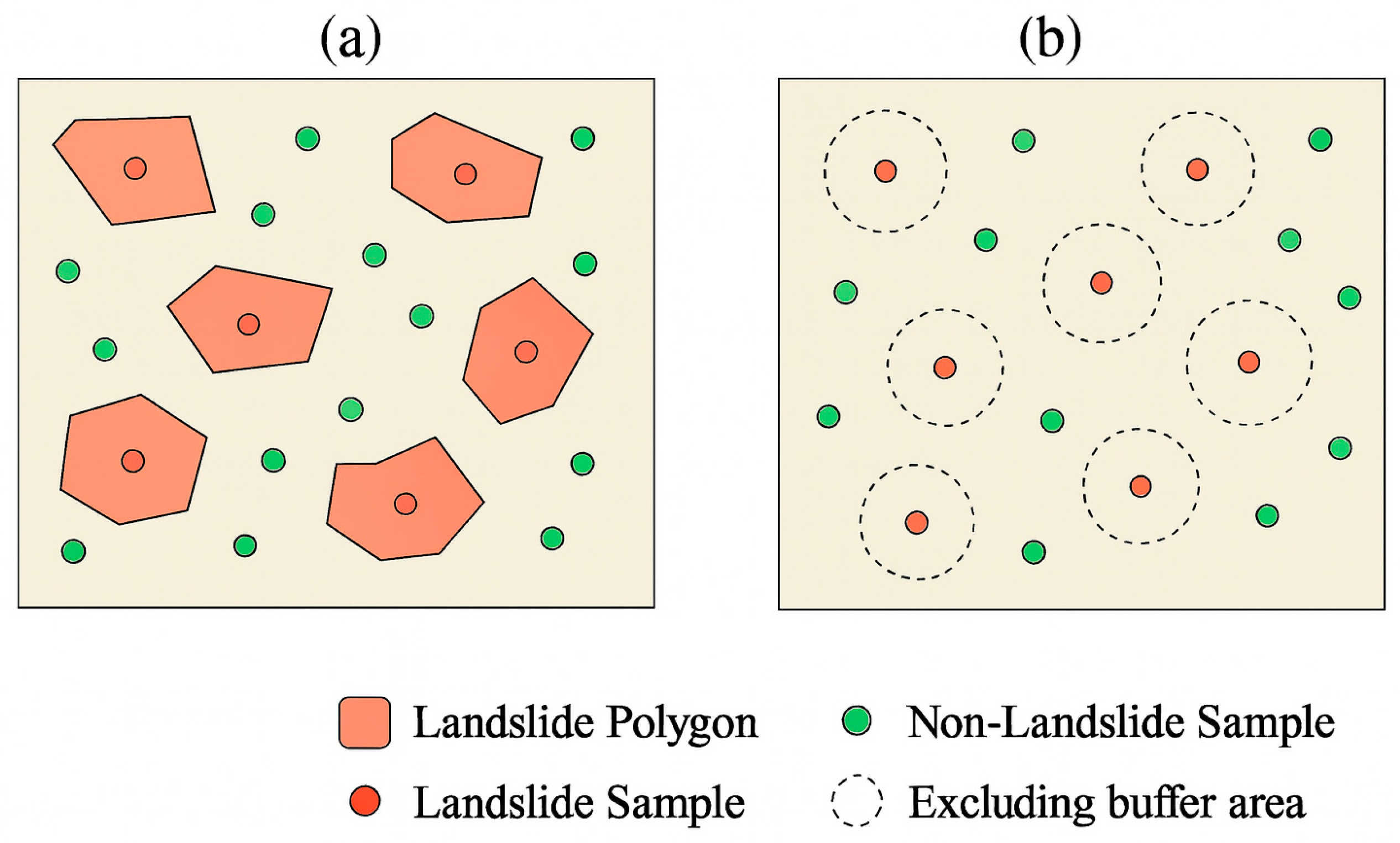
2.2. Landslide and Non-Landslide Data Sampling

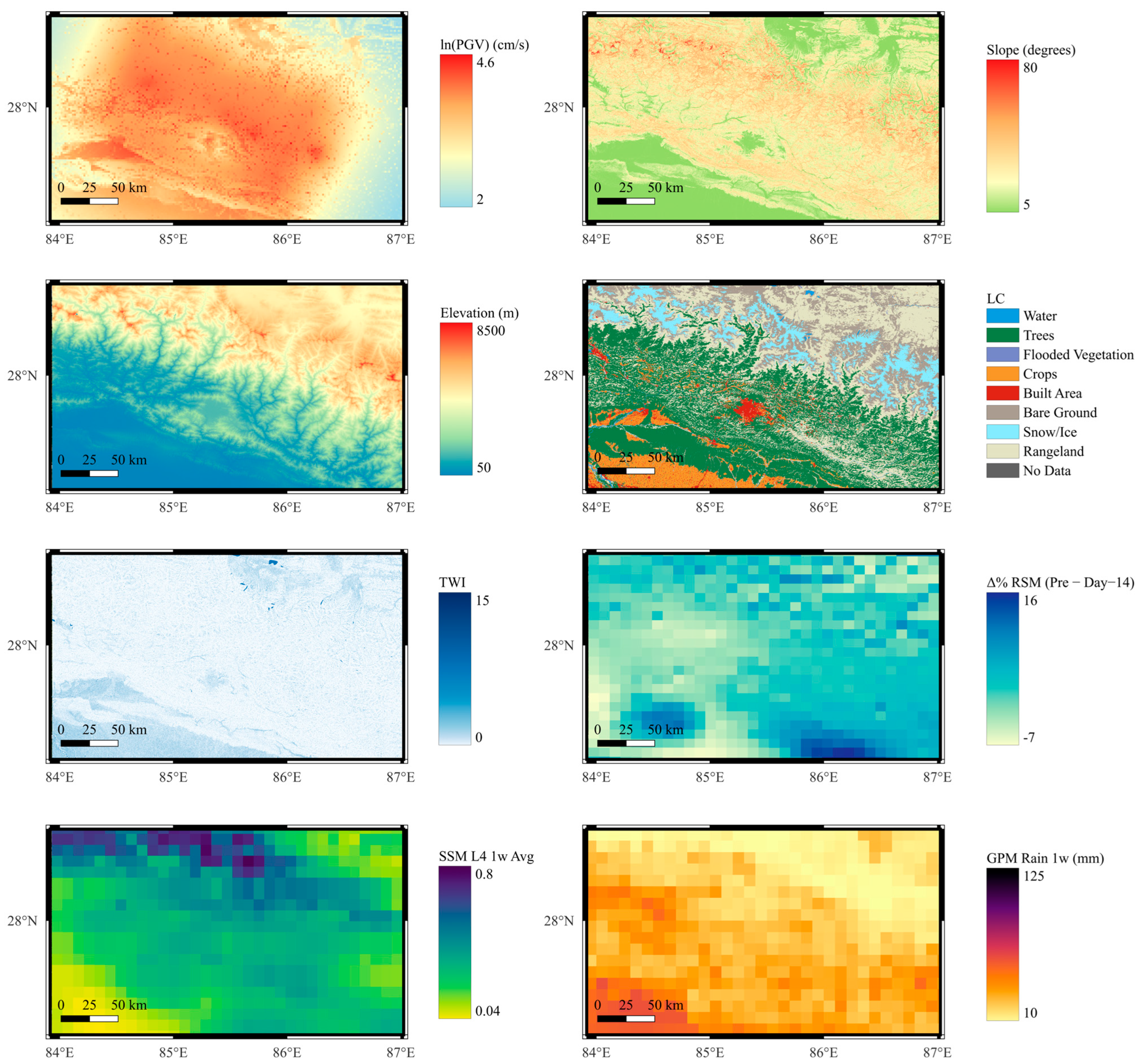
To construct a balanced and spatially controlled landslide modeling dataset, landslide (L) and non-landslide (NL) points were sampled for each earthquake using a consistent approach tailored to the format of each inventory. In the cases of Nepal and Indonesia, source points corresponding to the initiation zones of mapped polygons were available and directly used as landslide samples (24,843 and 7063 points, respectively). For New Zealand and Papua New Guinea, where source points were not provided, central interior points of the landslide polygons were extracted and used as proxies for landslide initiation locations (14,412 and 11,610 points, respectively). While centroid usage introduces some spatial uncertainty, this approach is consistent with previous studies [89] when source points are unavailable. In all polygon-based inventories, an equal number of NL points were randomly sampled within the mapped areas shown by light blue line in Figure 1, ensuring they were located outside both mapped landslide polygons and any obscured areas (e.g., cloud cover or data gaps). This spatial constraint helps reduce mislabeling and ensures more reliable non-landslide representation by sampling only within areas of confirmed inventory coverage.

As mentioned before, the Haiti inventory consists of 4893 landslide points. To address the incompleteness of this point-based inventory, an equal number of non-landslide samples were randomly selected within the mapped extent, excluding areas within an 85 m radius around each landslide point. This buffer approximates the average footprint of mapped landslides and was empirically derived from the 95th percentile of mapped polygon radii proposed by Nowicki Jessee et al. [27]. The sampling strategy for landslide (L) and non-landslide (NL) points based on inventory type is illustrated in Figure 2.

Across all events, a 1:1 L/NL ratio was maintained. While this ratio does not reflect real-world landslide prevalence [28], it supports balanced model learning—especially for binary classifiers—avoids bias toward the dominant non-landslide class, and allows consistent performance comparisons across models and case studies [27,62,66]. Furthermore, a study conducted by Yang et al. [128] shows that increasing the L/NL ratio beyond 1:1 does not necessarily lead to significantly better evaluation metrics.

Table 1. Summary of landslide database.

Landslide Inventory	Magnitude	Area Exposed to Landslides (km2)	Number of Landslide Cases	Number of Non-Landslide Cases
Nippes, Haiti 2021	7.2	4000	4893	4893
Palu, Indonesia 2018	7.5	4000	7063	7063
Tari, Papua New Guinea 2018	7.5	24,000	11,610	11,610
Kaikoura, New Zealand 2016	7.8	10,000	14,412	14,412
Gorkha, Nepal 2015	7.8	30,000	24,843	24,843

presents a summary of the selected earthquake events, including their magnitude, area exposed to landslides, and the number of landslide and non-landslide samples for each event. To ensure consistency and prevent overrepresentation of inventories with larger sample sizes—such as Nepal and New Zealand—the number of landslide and non-landslide cases from each event was down-sampled to match the smallest inventory (Haiti, with 4893 landslide and 4893 non-landslide cases). This approach maintains balance across datasets, mitigates model bias toward data-rich events.

2.3. Key Variables

Earthquake-induced landslides are governed by a combination of three major classes of variables: (1) topographic and geological factors, (2) seismic loading characteristics, and (3) hydrologic or wetness-related conditions. The inclusion of representative variables from each of these categories is essential to capture the mechanisms of slope failure. Depending on the spatial scale of the model, the availability of high-resolution input data may vary. For example, while regional models can incorporate detailed geotechnical datasets, such granularity is not typically accessible at continental or global scales. Therefore, globally available geospatial and satellite-based data products were selected to represent each class of explanatory variables across all earthquake regions included in this study.

Topographic and Geological variables describe terrain characteristics and subsurface conditions. Elevation, slope, Topographic Position Index (TPI), and Terrain Ruggedness Index (TRI) were extracted from digital elevation models (DEMs). Shear wave velocity over the top 30 m layer (V_S30) can also be considered as a proxy for soil physical properties. Moreover, land cover (LC) data was used to represent vegetation and built environments, both of which influence slope hydrology and failure susceptibility. To characterize earthquake ground motion, three intensity measures are commonly used: Peak Ground Velocity (PGV), Peak Ground Acceleration (PGA), and Modified Mercalli Intensity (MMI). These parameters are often interrelated and serve as proxies for the strength of ground shaking.

In the case of wetness-related variables, which is the focus of this study, variables that account for both long-term and short-term hydrologic influences are involved. Some of these are indirect proxies for soil saturation and include Topographic Wetness Index (TWI), Stream Power Index (STI), and historical mean annual precipitation [27,89]. While widely used in landslide studies, these proxies do not fully reflect the temporal variability in soil moisture conditions, which is critical to slope stability under dynamic seismic loading [51,59]. To address this gap, two satellite-derived data products were used; the Global Precipitation Measurement (GPM) [129] and Soil Moisture Active Passive (SMAP) [111] missions. GPM provides high-resolution precipitation measurements through its Integrated Multi-Satellite Retrievals for GPM (IMERG) algorithm, which fuses data from a constellation of satellites. The Final Run Version 07 Level-3 product, incorporating bias correction with rain gauge data, was used in this study. Accumulated rainfall data were processed over four key timeframes before each event, i.e., one year, one month, one week, and three days. Accumulated rainfall data were processed over four key timeframes before each event—one year, three months, one month, two weeks, and one week—as listed in

Table 2. Summary of key variables.

Category	Variable Name (s)	Source
Topographic and Geological	Elevation, Slope, TRI, TPI	Digital Elevation Model (STRM)
	VS30	[131]
	Land Cover	Esri Sentinel-2
Ground Shaking Intensity	PGA, GV	USGS
Wetness Proxies	TWI, STI	Digital Elevation Model (STRM)
	Historical Precip	World Clim database
GPM precipitation	GPM Rain 1yr, 3mo, 1mo, 2w, 1w	Giovanni
SMAP—Prior-event Normalized Soil Moisture	RSM 1mo Avg, 2w Avg, 1w Avg, 3d Avg SSM L4 1mo Avg, 2w Avg, 1w Avg, 3d Avg SSM L3 1mo Avg, 2w Avg, 1w Avg RSM Pre, SSM L4 Pre, SSM L3 Pre	National Snow and Ice Data Center
SMAP—Short-Term Change Ratio	%Δ RSM (Pre − 1w Avg), RSM (3d Ave − 2w Avg), %Δ RSM (3d Ave − 1mo Avg) %Δ SSM L4 (Pre − 1w Avg), %Δ SSM L4 (3d Ave − 2w Avg), %Δ SSM L4 (3d − 1mo)
SMAP—Lag-Based Changes	%Δ SSM L4 (Pre − Day−3/7/10/14), %Δ RSM (Pre − Day−3/7/10/14)

(e.g., GPM Rain 1yr, 3mo, 1mo, 2w and 1w). All GPM precipitation data were downloaded from the NASA Giovanni portal [130].

SMAP is a NASA mission providing global soil moisture observations. It includes Level 3 surface soil moisture (SSM) data retrieved from passive radiometer measurements at 6:00 a.m. or 6:00 p.m. LST. Only 6:00 a.m. retrievals were used in this study to minimize diurnal variation effects [58]. This data product has a grid resolution of 9 km on Equal-Area Scalable Earth Grid 2.0 (EASE-Grid 2.0) and a 3-day average temporal resolution. Version 6 of the product was used in this study, which is freely available from the National Snow and Ice Data Center (NSIDC) in Hierarchical Data Format version 5 (HDF5). Level 4 soil moisture data include surface and root-zone soil moisture (RSM) estimates. These are derived by assimilating SMAP observations into land surface models, offering enhanced temporal resolution (3-hourly) and better continuity in regions or times where Level 3 data may be missing. The soil moisture variables derived from SMAP were categorized into three thematic groups to better capture temporal dynamics and changes leading up to the earthquake:

(1)

Prior-event Normalized Soil Moisture: Averages of Root Zone Soil Moisture (RSM), Level 4 Surface Soil Moisture (SSM L4), and Level 3 Surface Soil Moisture (SSM L3) were computed over multiple pre-event windows (1 month, 2 weeks, 1 week, and 3 days). Due to temporal resolution limitations, a 3-day average was not computed for Level 3. In addition to antecedent conditions, RSM and SSM L4 values were also extracted for the day of the earthquake to represent modeled soil moisture at the time of shaking. For SMAP L3, the nearest-available value was used when event-day data were unavailable due to its coarser temporal sampling schedule. Each soil moisture value, whether from antecedent or event-day windows, was normalized using the annual minimum and maximum soil moisture values for the corresponding earthquake year, following:

$${SM}_{norm}={\displaystyle \frac{SM-{SM}_{min}}{{SM}_{max}-{SM}_{min}}}$$

(1)

where $SM$ is soil moisture value, and ${SM}_{min}$ and ${SM}_{max}$ represent the minimum and maximum annual values. These normalized metrics characterize relative wetness conditions and baseline soil saturation across different periods prior to each earthquake, which can influence pore pressure buildup and slope strength over time.

(2)

Short-Term Soil Moisture Change: These variables quantify the percentage change in soil moisture over short-term periods leading up to the earthquake, specifically for Root Zone Soil Moisture (RSM) and Level 4 Surface Soil Moisture (SSM L4). The change is calculated between the 3-day average prior to the event and longer-term antecedent averages (1 month and 2 weeks), as well as between the event-day value and the 1-week average. These variables assess whether soils were experiencing anomalous wetting or drying prior to failure and destabilizing conditions such as post-rainfall infiltration, offering insight into potential triggering mechanisms.

(3)

Lagged Soil Moisture Change: Percent differences in Root Zone Soil Moisture (RSM) and Level 4 Surface Soil Moisture (SSM L4) were computed between event-day values and those recorded at lagged time steps (e.g., 3, 7, 10, and 14 days before the earthquake). These changes capture the short-term evolution of soil moisture, allowing detection of rapid wetting or drying trends that may not be evident in longer-term averages. Such variations can help identify transient hydrologic conditions conducive to slope failure under seismic loading.

Table 2 summarizes all the input variables used in the study, along with their definitions and data sources. To address resolution differences among input variables, values for each variable were extracted at landslide and non-landslide (L/NL) point locations using the native resolution of the corresponding raster dataset via nearest-neighbor sampling. This strategy preserves the spatial integrity of each dataset (e.g., 9 km for SMAP, ~10 km for GPM, and finer resolutions for DEM-derived layers) and avoids uncertainties associated with resampling during data extraction.

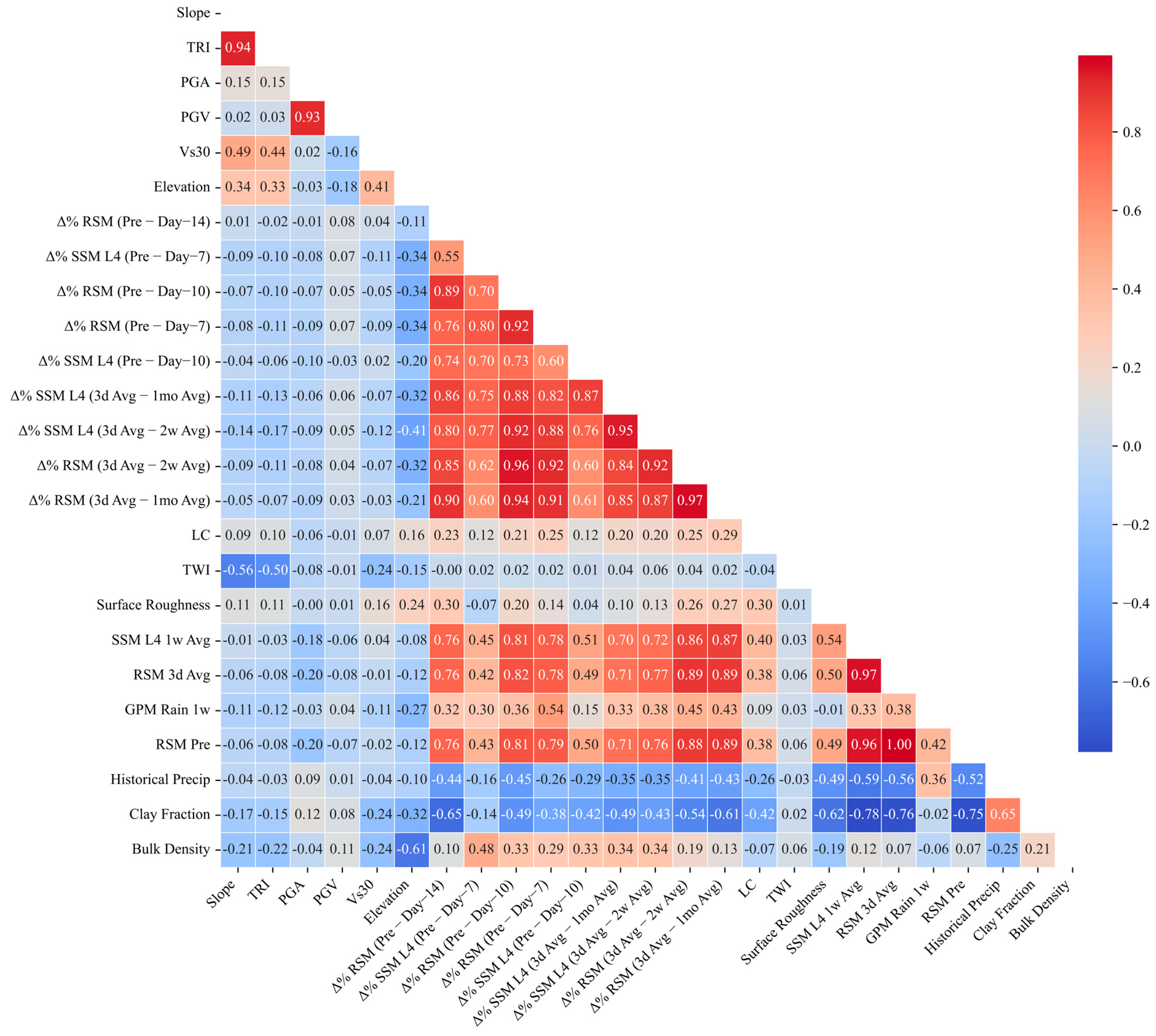
2.4. Independent Variable Selection and Multicollinearity Test

To select meaningful and non-redundant predictor variables for landslide susceptibility modeling, a multi-step feature selection process was employed. First, the Pearson correlation coefficient was calculated between each continuous variable and the binary landslide occurrence label for each individual earthquake. For the categorical variable land cover (LC), the Cramér’s V statistic was used instead [27], as it is more appropriate for measuring association between categorical and binary variables. Variables with a correlation coefficient greater than 0.2 in at least two separate events were retained for further analysis. This step served to filter out weakly associated predictors while allowing some flexibility for cross-event variability. The retained variables and their correlation coefficients are illustrated in Figure 3, where only coefficients exceeding 0.2 are shown. This choice reflects a balance between filtering out weak predictors and retaining variables that may have moderate yet consistent influence across diverse events [27]. Given the variability in landslide-triggering mechanisms and environmental conditions, a 0.2 threshold helps capture more generalizable signals without allowing noise-dominated features into the model. Next, to assess pairwise collinearity, a correlation matrix was computed using the combined dataset of all earthquakes. As shown in Figure 4, pairs of variables with high correlation coefficients (greater than 0.8) were considered collinear. In each such case, only one variable was retained, prioritizing interpretability, physical relevance, and consistency across events. This step ensured that strongly redundant variables did not enter the model simultaneously.

To further address multicollinearity among the remaining variables, the Variance Inflation Factor (VIF) was computed. VIF quantifies how much the variance of an estimated regression coefficient increases due to collinearity. A VIF value greater than 10 is commonly considered problematic [89]. The final set of variables retained after this filtering step is presented in

Table 3. Multicollinearity analysis of selected variables after filtering out redundant or highly correlated variables.

Variable	VIF
PGV	8.2
Slope	7.1
Elevation	3.4
LC	2.9
TWI	1.8
Δ% RSM (Pre – Day–14)	2.9
SSM L4 1w Avg	7.8
GPM Rain 1w	4.1

, along with their corresponding VIF values. The selected variables include both seismic and geospatial predictors such as Peak Ground Velocity (PGV), slope, elevation, and land cover (LC), along with several soil moisture and precipitation-related variables: Topographic Wetness Index (TWI); Δ% RSM (Pre − Day–14), which represents the percent change in Root Zone Soil Moisture from 14 days before the event to the day prior; SSM L4 1w Avg, the 1-week average of Surface Soil Moisture from SMAP Level 4 prior to the event; and GPM Rain 1w, the total accumulated rainfall over one week before the event derived from GPM data. Figure 5 displays maps of selected explanatory variables for the Nepal earthquake data inventory, for example.

2.5. Model Development

Random Forest (RF) is a machine learning algorithm that builds many decision trees using random samples of the data [132,133]. Each tree makes a prediction, and the final result is based on the majority vote across all trees. During training, RF introduces randomness in two ways: by using different subsets of the data (bootstrapping) and by selecting a random group of predictor variables at each tree split. This randomness makes the model more robust and helps prevent overfitting, where a model performs well on training data but poorly on new data. In particular, RF reduces the risk of overfitting through ensemble averaging, which stabilizes predictions and mitigates the influence of noisy or overly complex individual trees.

RF is particularly well-suited for landslide susceptibility modeling for several reasons. It can capture complex, nonlinear relationships between input variables and landslide occurrence without requiring assumptions about data distribution. This is especially important given that landslide processes are driven by heterogeneous and interacting geospatial and geotechnical factors that are rarely linear. Random Forest performs well even with correlated or noisy predictors, as each decision tree considers only a random subset of features at each split—reducing the dominance of highly correlated variables and distributing their influence across the ensemble. It also handles both continuous and categorical data without requiring prior transformation. It also includes an inherent mechanism for estimating variable importance—providing insight into the relative contribution of each predictor to the classification task. For these reasons, the RF algorithm was chosen as the core modeling tool in this study to predict earthquake-induced landslide susceptibility using a combination of seismic, hydrological, and terrain variables. In this study, the Random Forest model was implemented using 50 trees, a maximum tree depth of 16, and a minimum of 4 samples required to split an internal node, following optimal hyperparameter settings identified in previous landslide studies [134].

Two modeling strategies were implemented to assess landslide susceptibility across multiple earthquake events. The first approach involved training a global model using the full dataset (24,465 landslide and 24,465 non-landslide samples), combining equal contributions from all five earthquakes. In this setup, the dataset was randomly split into 70% for training and 30% for testing, ensuring that the model was exposed to a wide range of spatial and geological conditions during training. The second approach adopted a leave-one-earthquake-out cross-validation framework to assess model generalizability. In this strategy, data from four earthquakes were used for training, while the fifth event was reserved for testing. This process was repeated five times, with each earthquake serving once as the unseen test set. This simulates the realistic challenge of applying a model trained on past events to predict landslide susceptibility in a new, unobserved earthquake scenario.

Model performance was evaluated on the test set for both the global model (30% holdout) and the held-out event in the leave-one-earthquake-out cross-validation framework. A suite of standard classification metrics was used: $Accuracy$, $Precision$, $Recall$, $F1\text{-}score$, and the Area Under the Receiver Operating Characteristic Curve (AUC). These metrics provide complementary perspectives on classification performance, which is especially important in the context of landslide prediction, where both false positives and false negatives carry significant consequences. The evaluation metrics are defined as follows:

• $Accuracy$: Overall proportion of correctly classified instances.

  $$Accuracy={\displaystyle \frac{TP+TN}{TP+TN+FP+FN}}$$

  (2)
• $Precision$: Proportion of predicted landslides that are true landslides.

  $$Precision={\displaystyle \frac{TP}{TP+FP}}$$

  (3)
• $Recall$ Sensitivity): Proportion of actual landslides correctly identified.

  $$Recall={\displaystyle \frac{TP}{TP+FN}}$$

  (4)
• $F1\text{-}score$: Harmonic mean of precision and recall, balancing both metrics.

  $$F1\text{-}score=2\times {\displaystyle \frac{Precision\times Recall }{Precision+Recall}}$$

  (5)
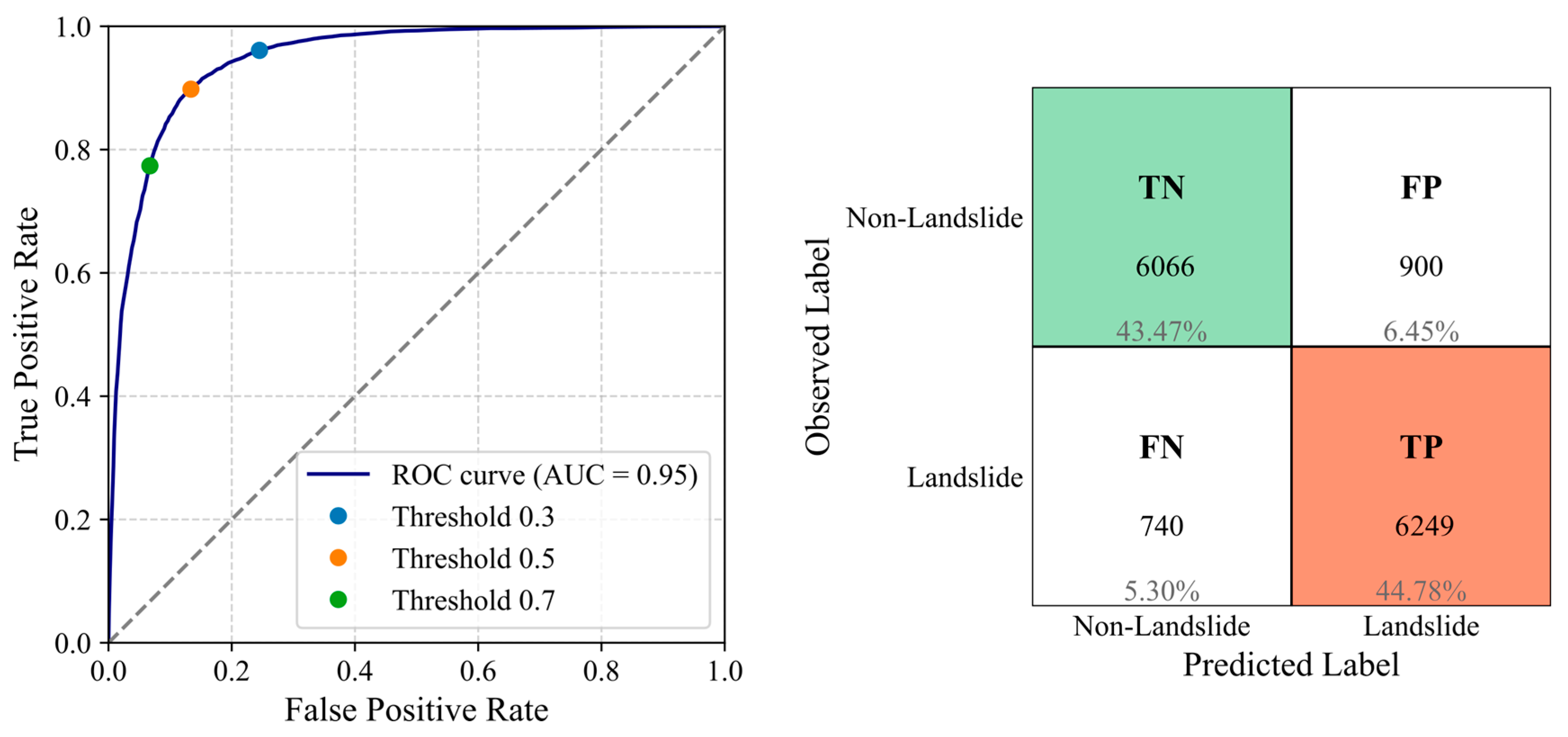
• AUC (Area Under the ROC Curve): The ROC (Receiver Operating Characteristic) curve plots the true positive rate (TPR)—the proportion of landslide cases correctly classified as landslides by the model—against the false positive rate (FPR)—the proportion of non-landslide cases incorrectly classified as landslides—across various classification thresholds. The AUC summarizes this curve into a single value, representing the model’s ability to distinguish between classes independently of any fixed threshold.

  $$TPR={\displaystyle \frac{TP}{TP+FN}}$$

  (6)

  $$FPR={\displaystyle \frac{FP}{TN+FP}}$$

  (7)

Here, TP stands for the number of True Positive cases (landslide events correctly predicted by the model), TN refers to True Negatives (non-landslide events correctly identified), FP indicates False Positives (non-landslide events incorrectly classified as landslides), and FN represents False Negatives (landslide events that the model failed to predict).

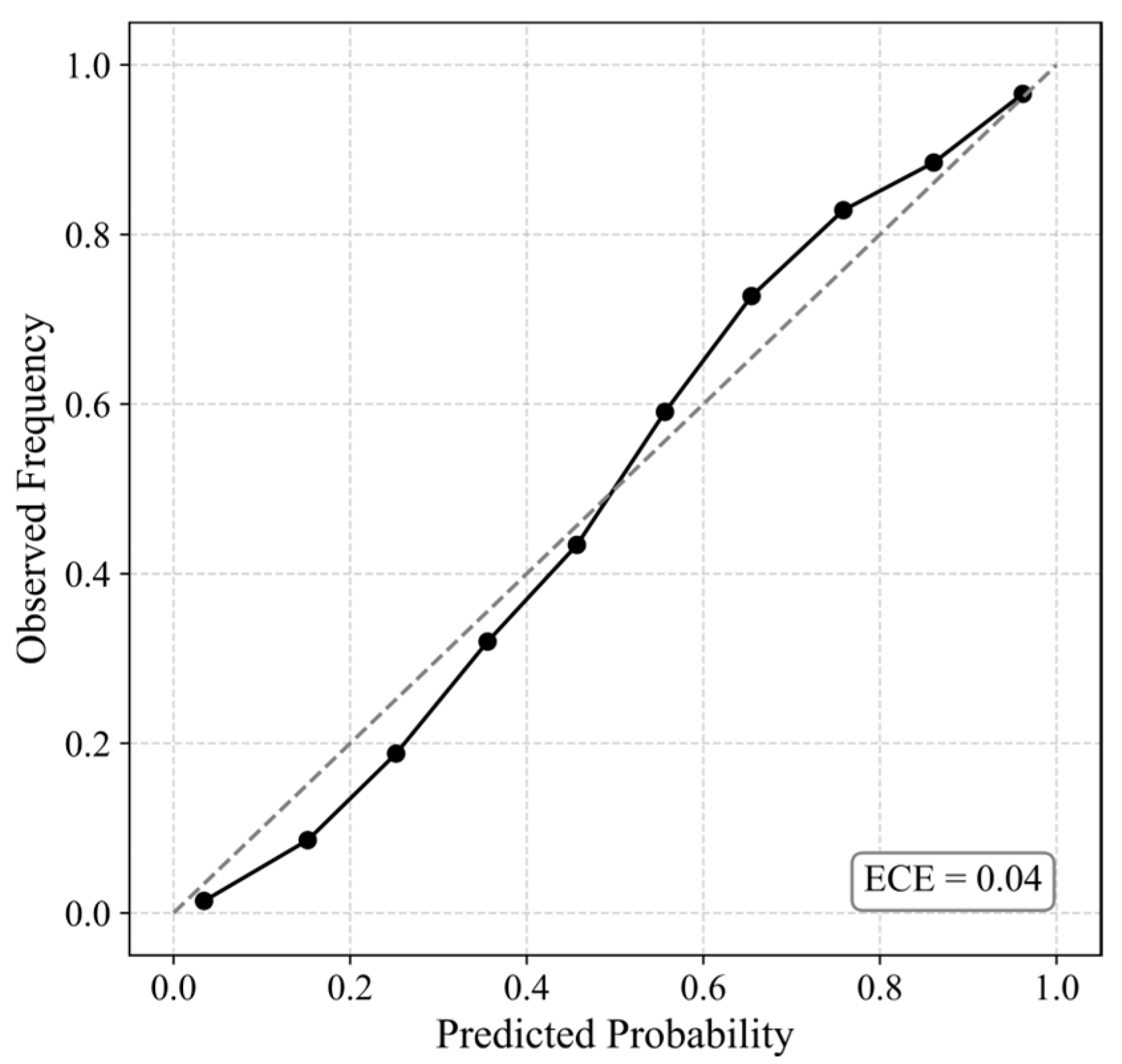
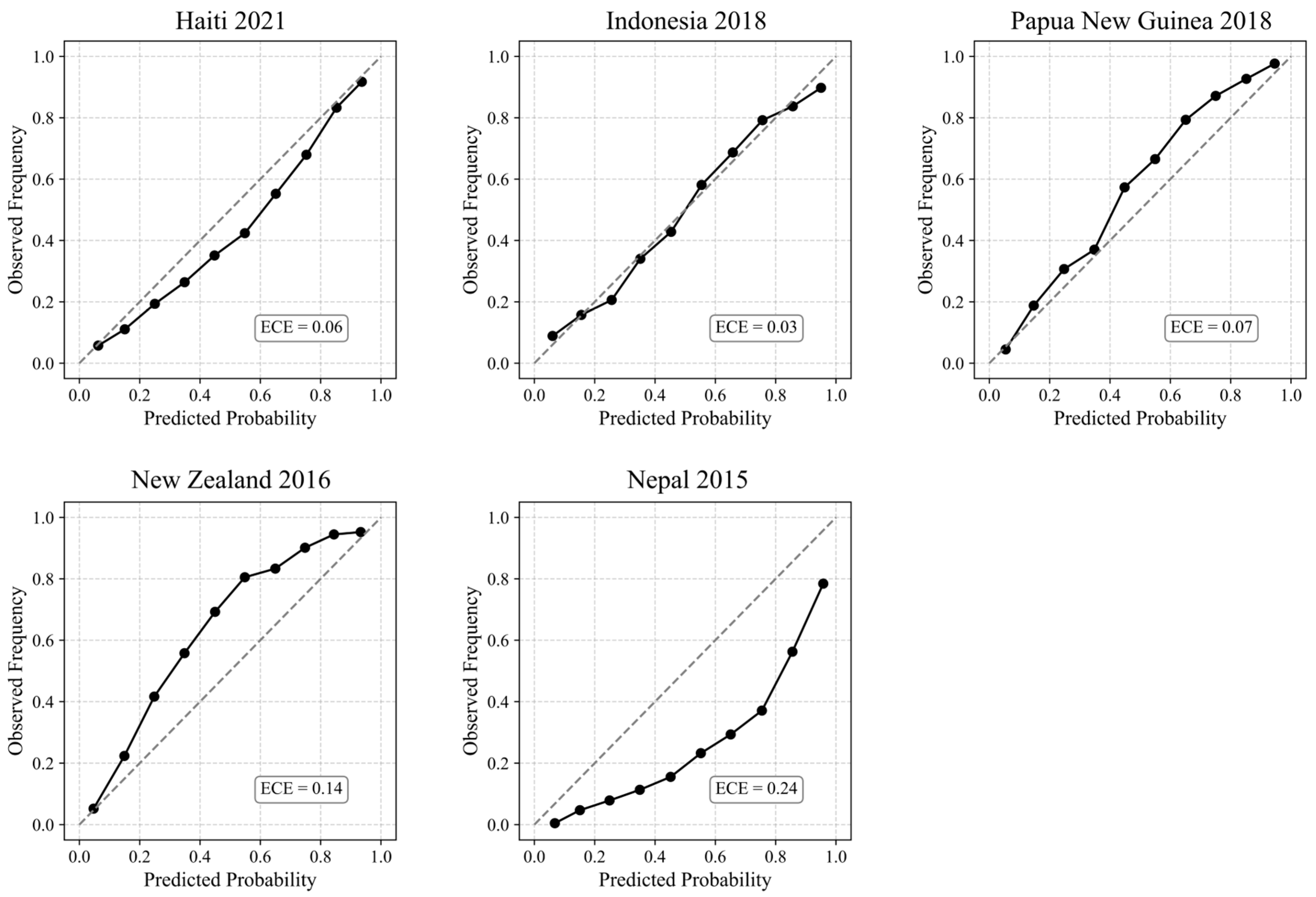
2.6. Assessment of Model Uncertainty and Reliability

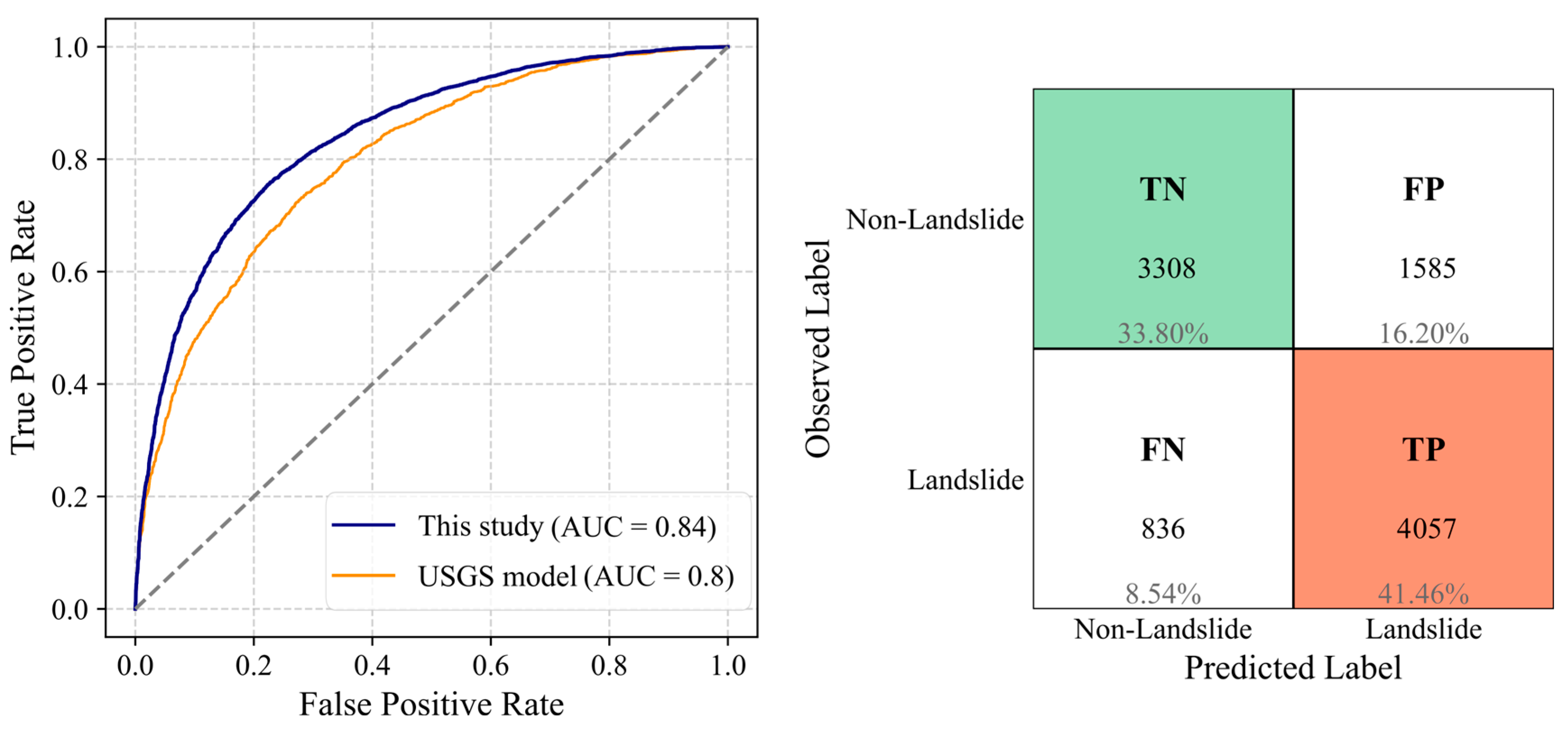
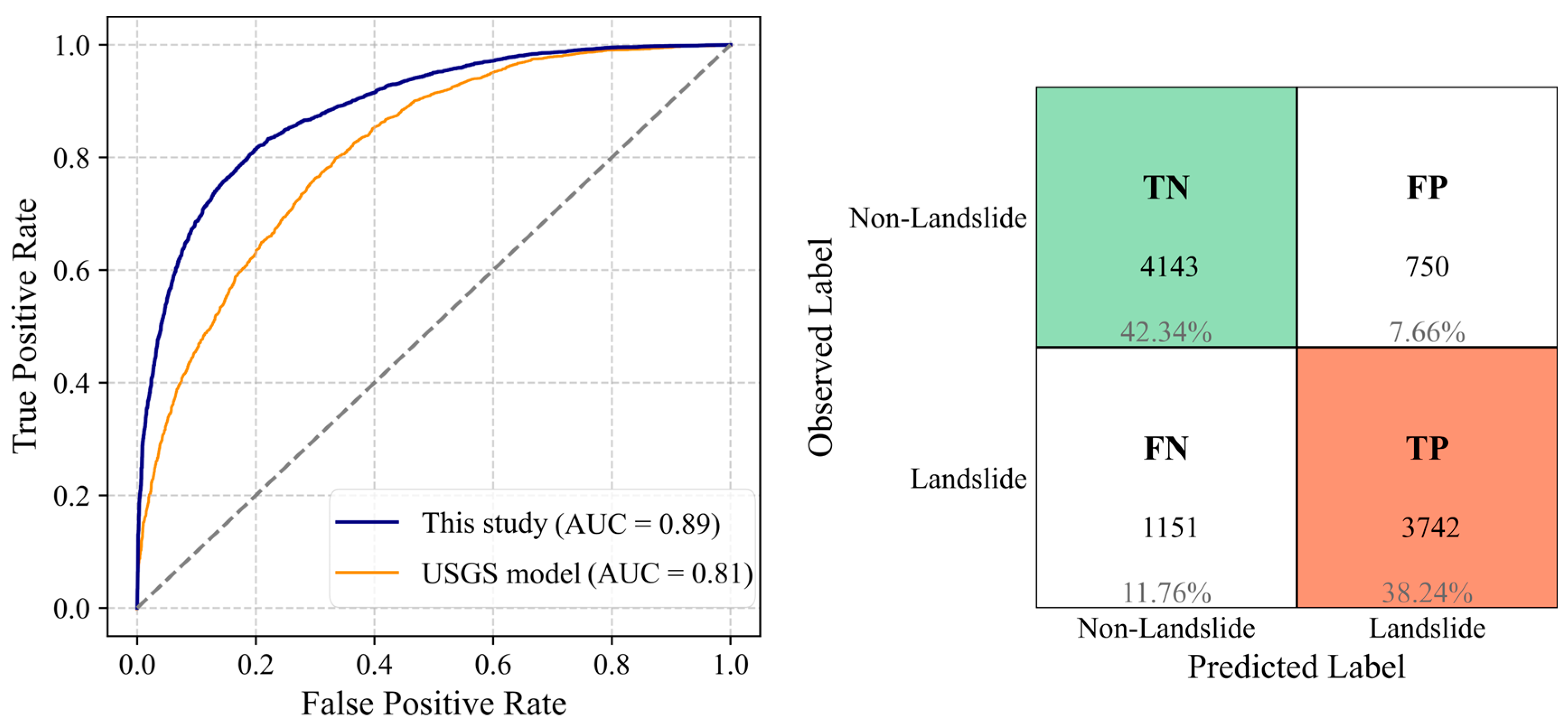
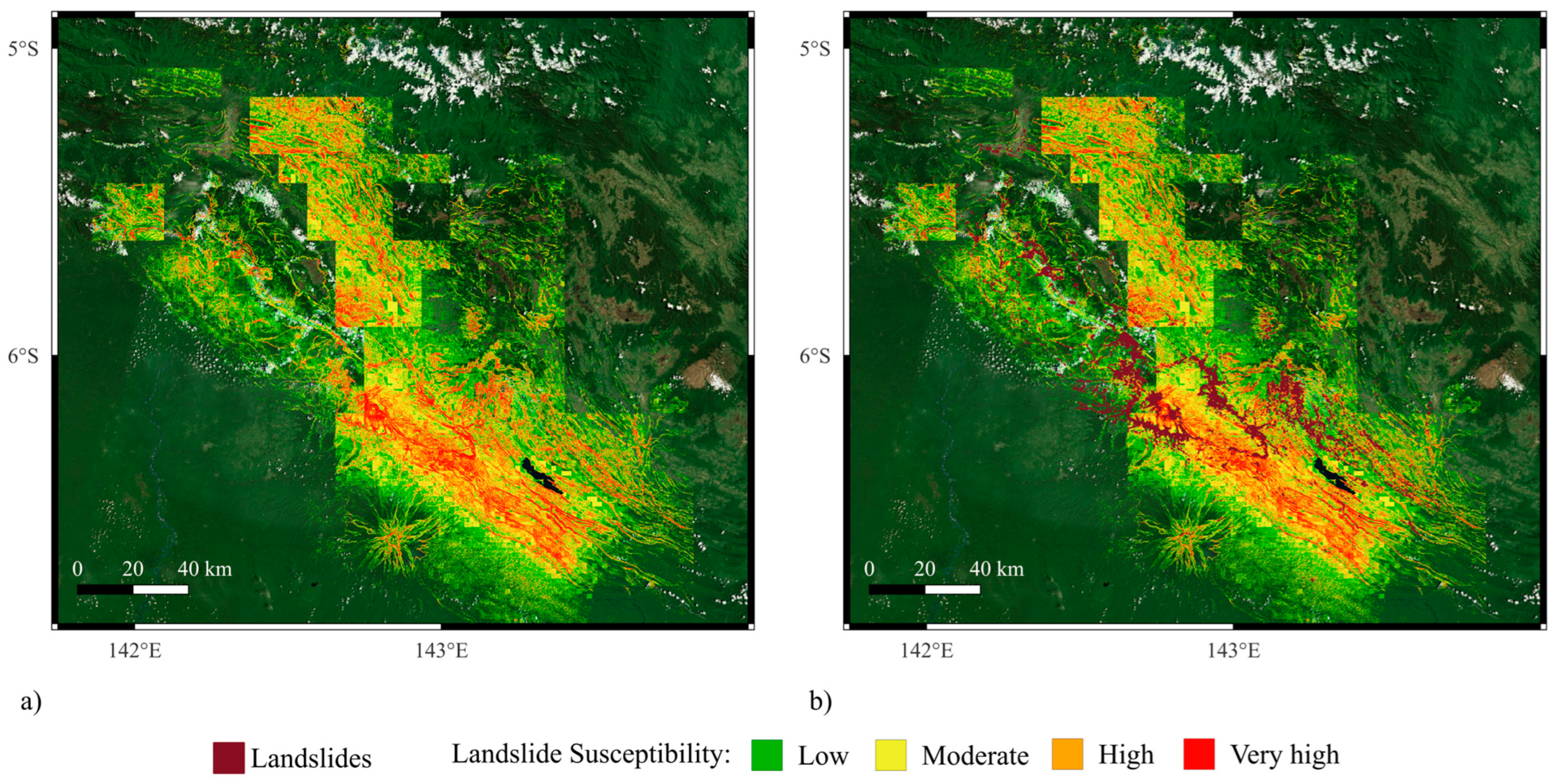
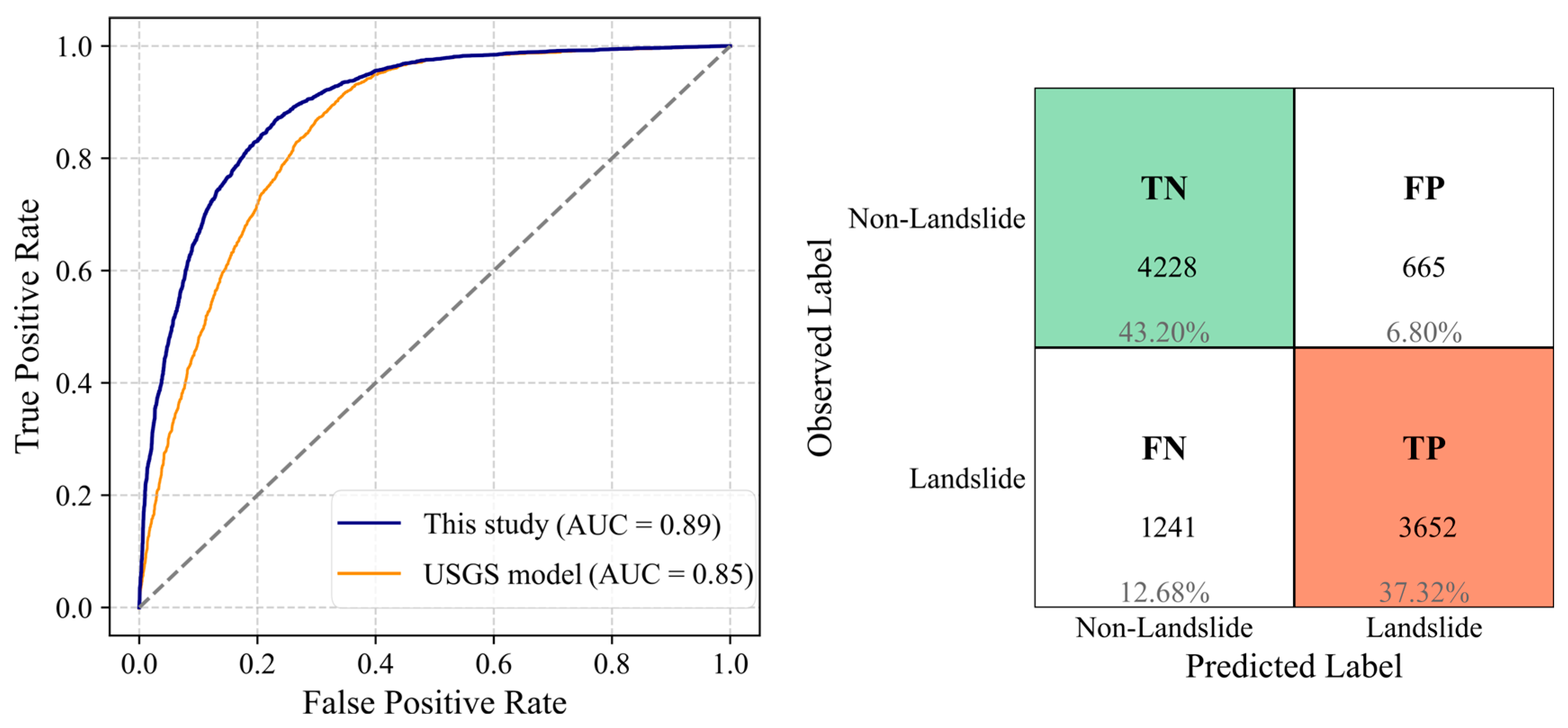
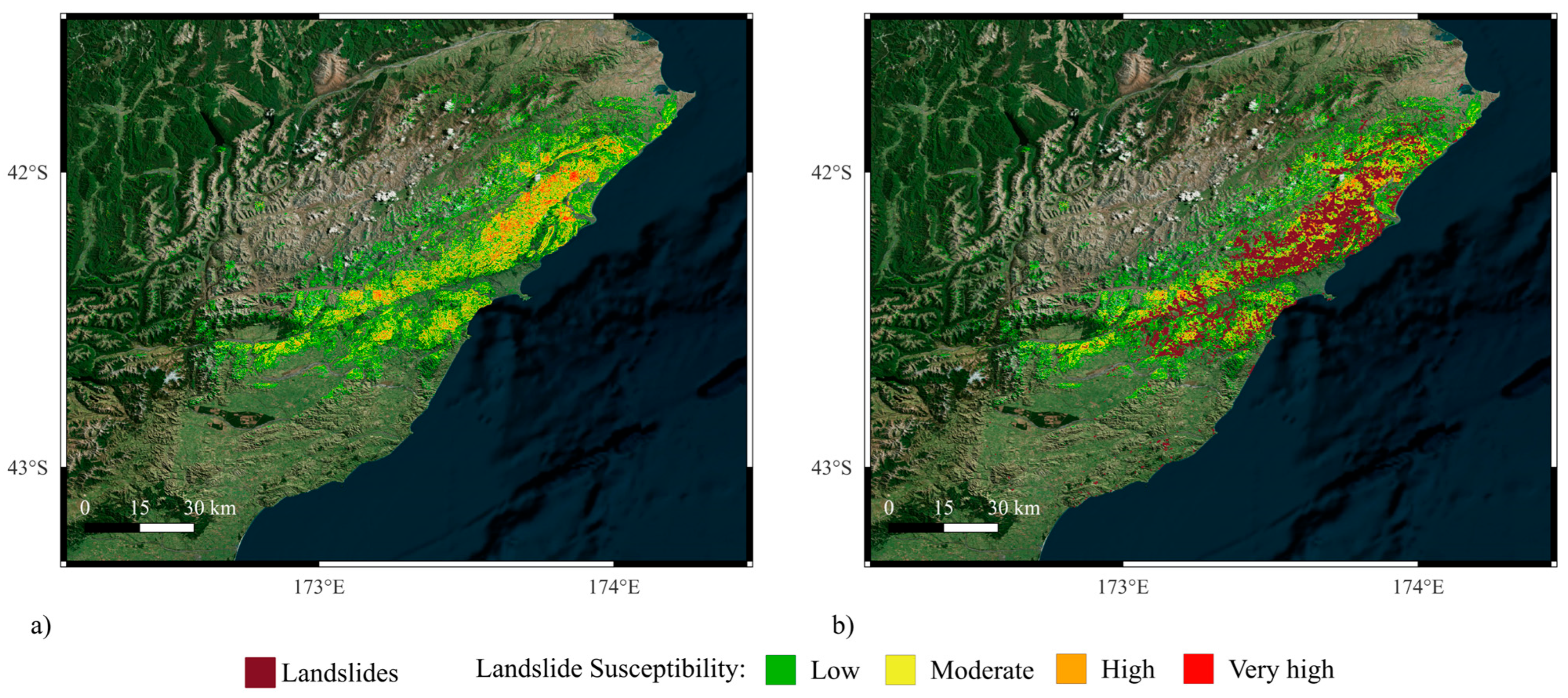
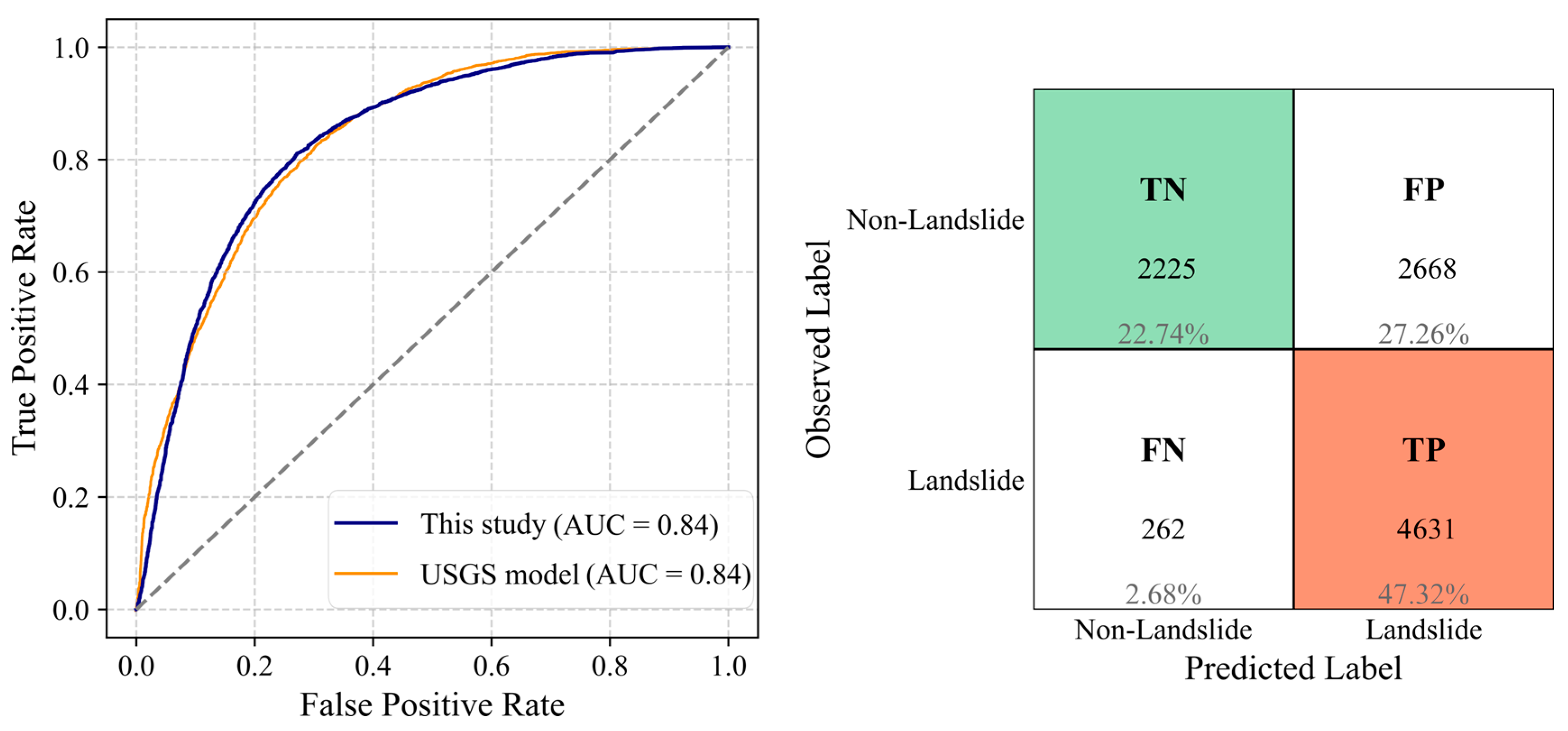
To assess the reliability and uncertainty of the probabilistic predictions, three complementary tools were used: the Brier Score [135], the Reliability Curve [136], and the Expected Calibration Error (ECE) [137]. The Brier Score is a proper scoring rule that evaluates the accuracy of probabilistic predictions. The Brier Score is defined as the mean squared difference between the predicted probabilities and the actual observed class labels (where 0 represents no landslide and 1 represents landslide occurrence):

$$Brier score={\displaystyle \frac{1}{n}}\sum _{i=1}^n{(\widehat{p_i}-y_i)}^2$$

(8)

where $\widehat{p_i}$ is the predicted probability for sample $i$, $y_i$ is the observed label, and $n$ is the total number of samples. A lower Brier Score indicates that the predicted probabilities are closer to the actual label, meaning the model is both better calibrated and more accurate in expressing its confidence about each prediction.

The Reliability Curve (also known as the calibration curve) provides a visual tool to assess whether predicted probabilities align with observed events (landslide and nonlandslide). Predictions are grouped into discrete probability bins (e.g., 0.0–0.1, 0.1–0.2, etc.). For each bin, the average predicted probability (x-axis) is plotted against the actual observed frequency of landslide occurrences in that bin (y-axis). A perfectly calibrated model would have all points lying on the diagonal line y = x, indicating that predicted probabilities correctly reflect actual risks.

To summarize the overall calibration behavior numerically, the Expected Calibration Error (ECE) was computed. ECE measures the weighted average difference between predicted probability and observed outcome frequency across bins. The formulation is:

$$ECE=\sum _{m=1}^M{\displaystyle \frac{\left|B_m\right|}{n}}·\left|acc\left(B_m\right)-conf\left(B_m\right)\right|$$

(9)

where M is the number of bins, ∣Bm∣ is the number of samples in bin m, acc(Bm) is the fraction of positive labels (landslide) in bin m (i.e., observed frequency), and conf(Bm) is the average predicted probability in bin m. Lower ECE values indicate better agreement between predicted probability and actual labels. Together, these metrics and plots provide a comprehensive understanding of the model’s uncertainty characteristics and the trustworthiness of its probability estimates.

3. Results

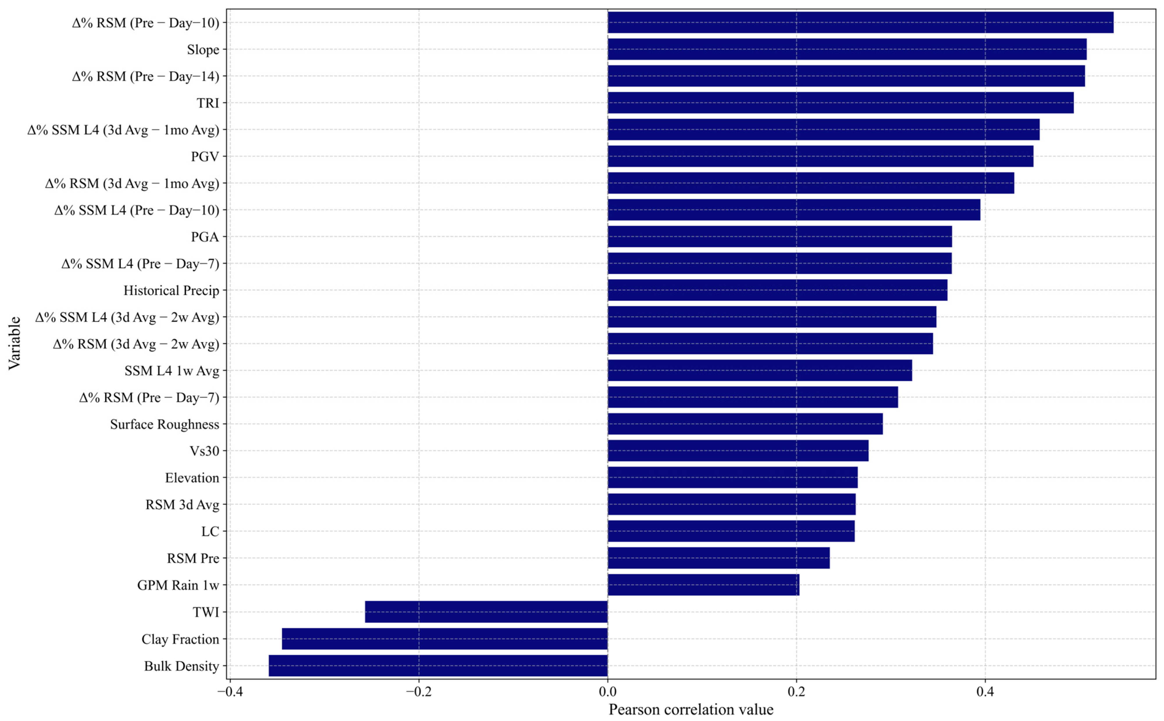
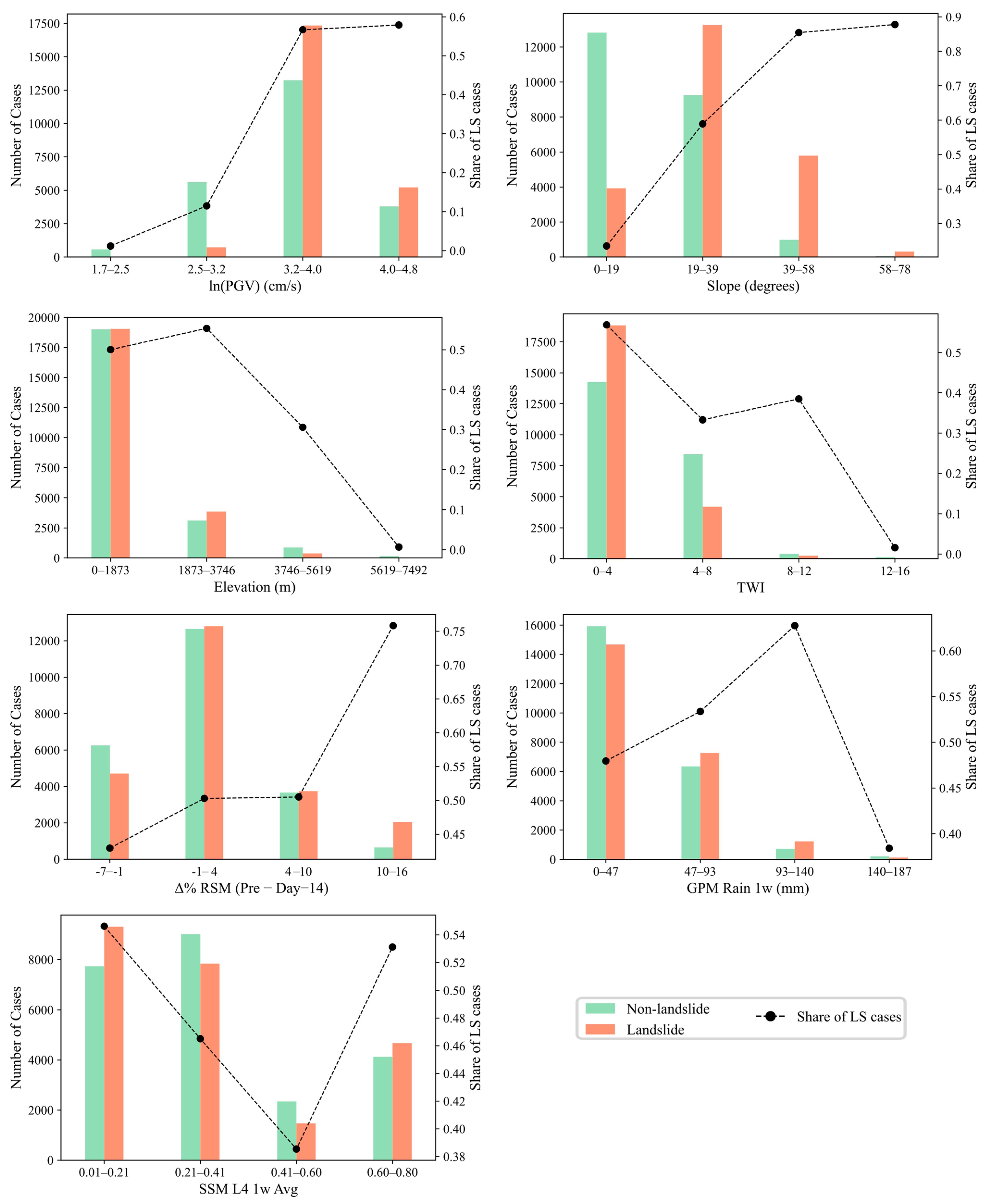
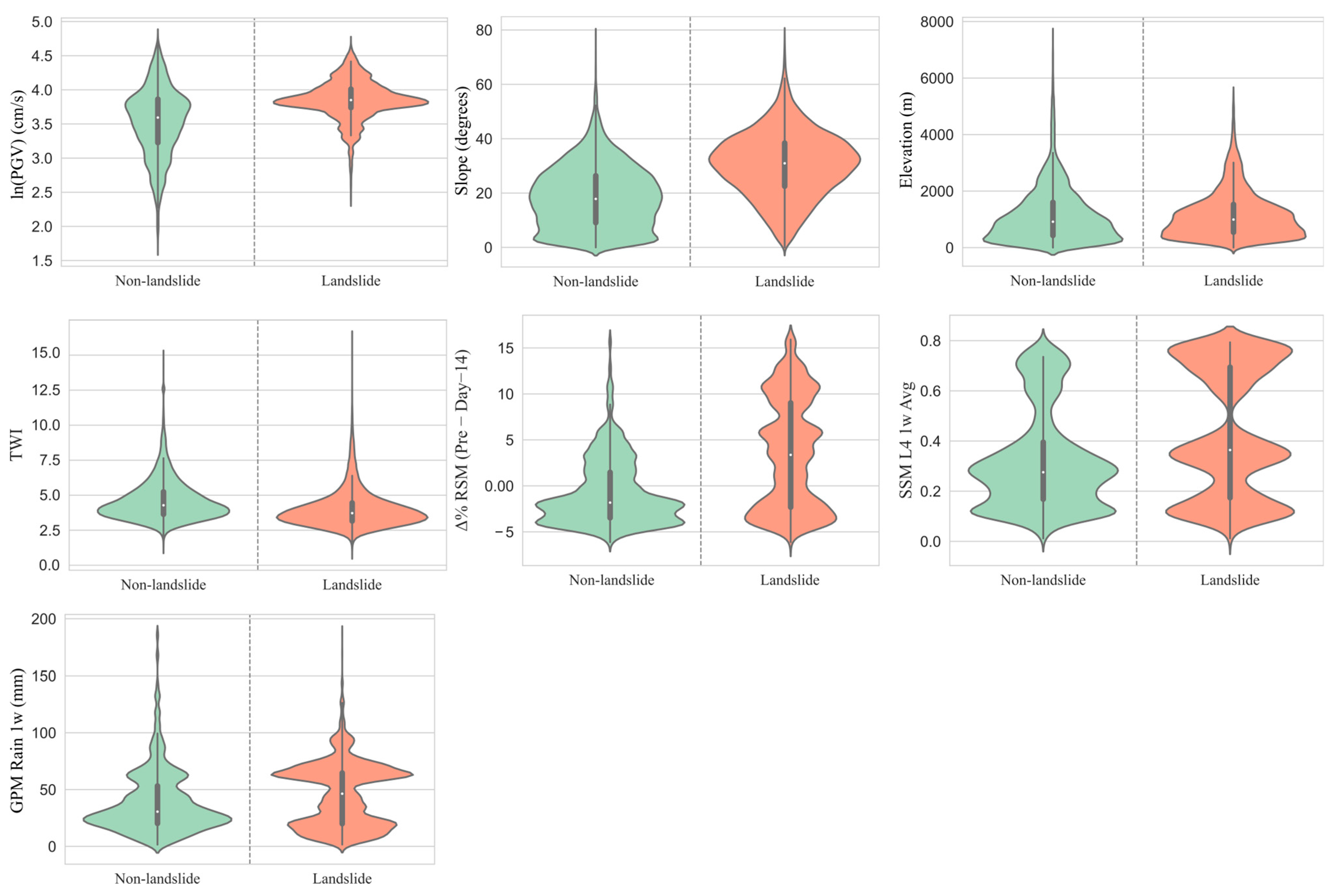
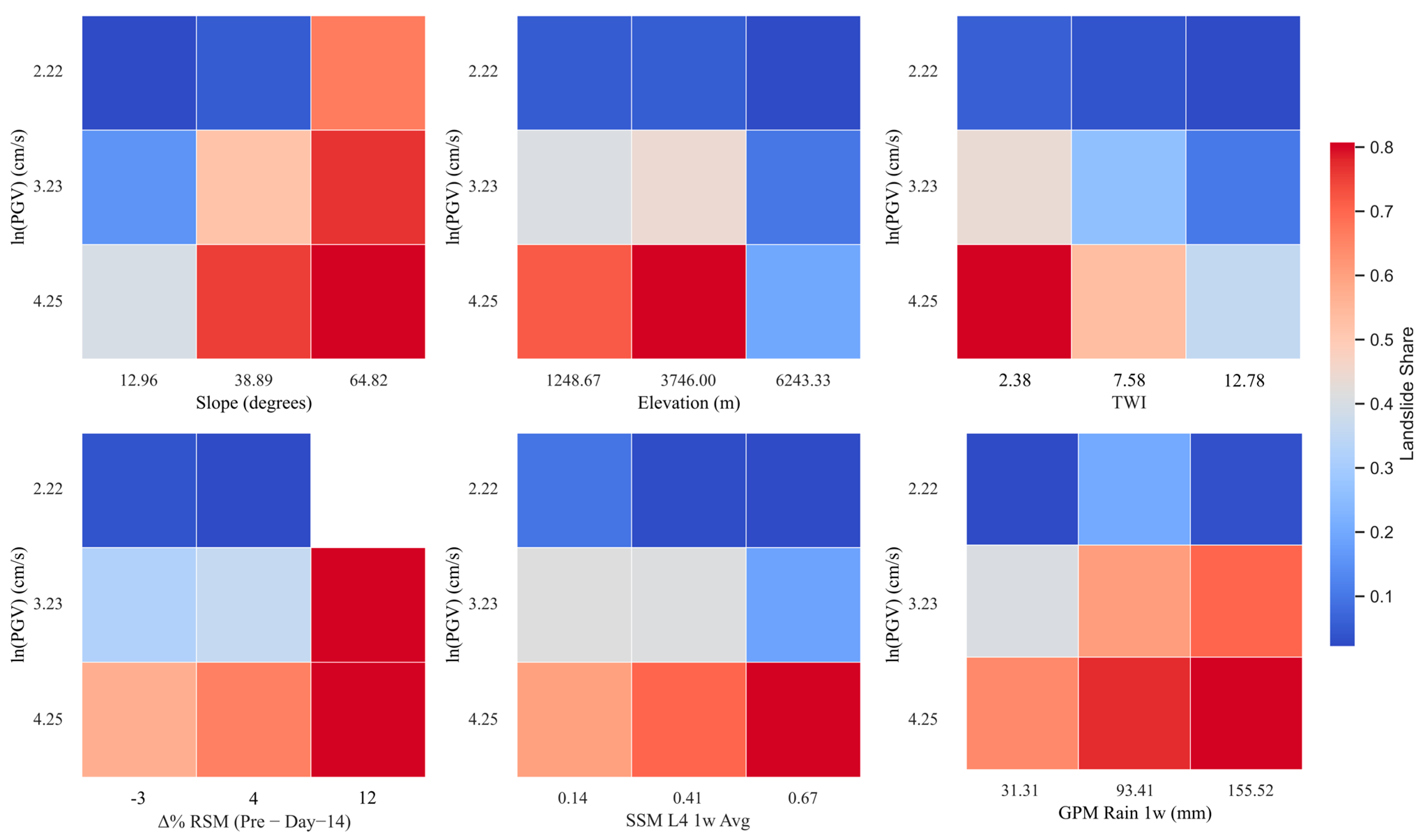
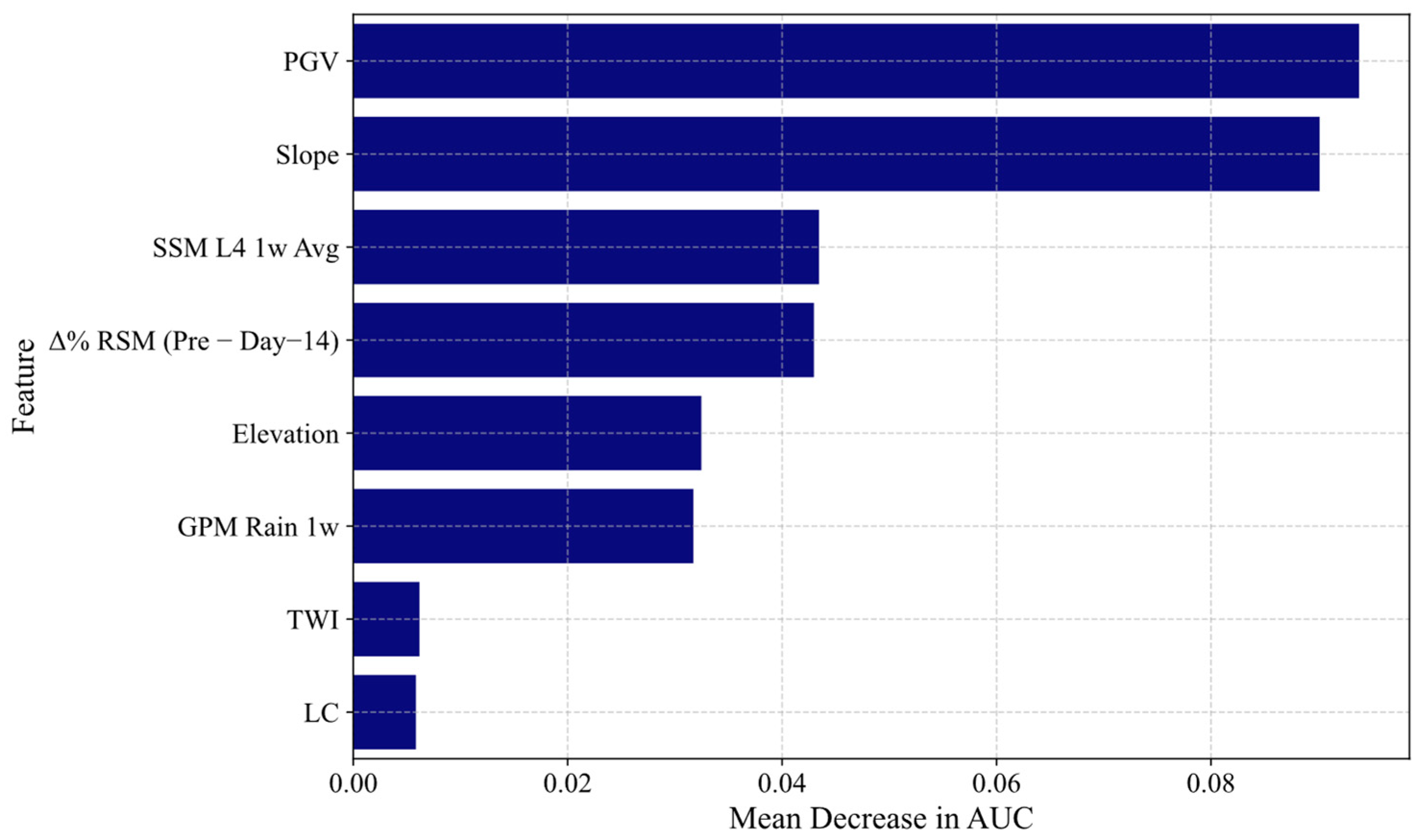
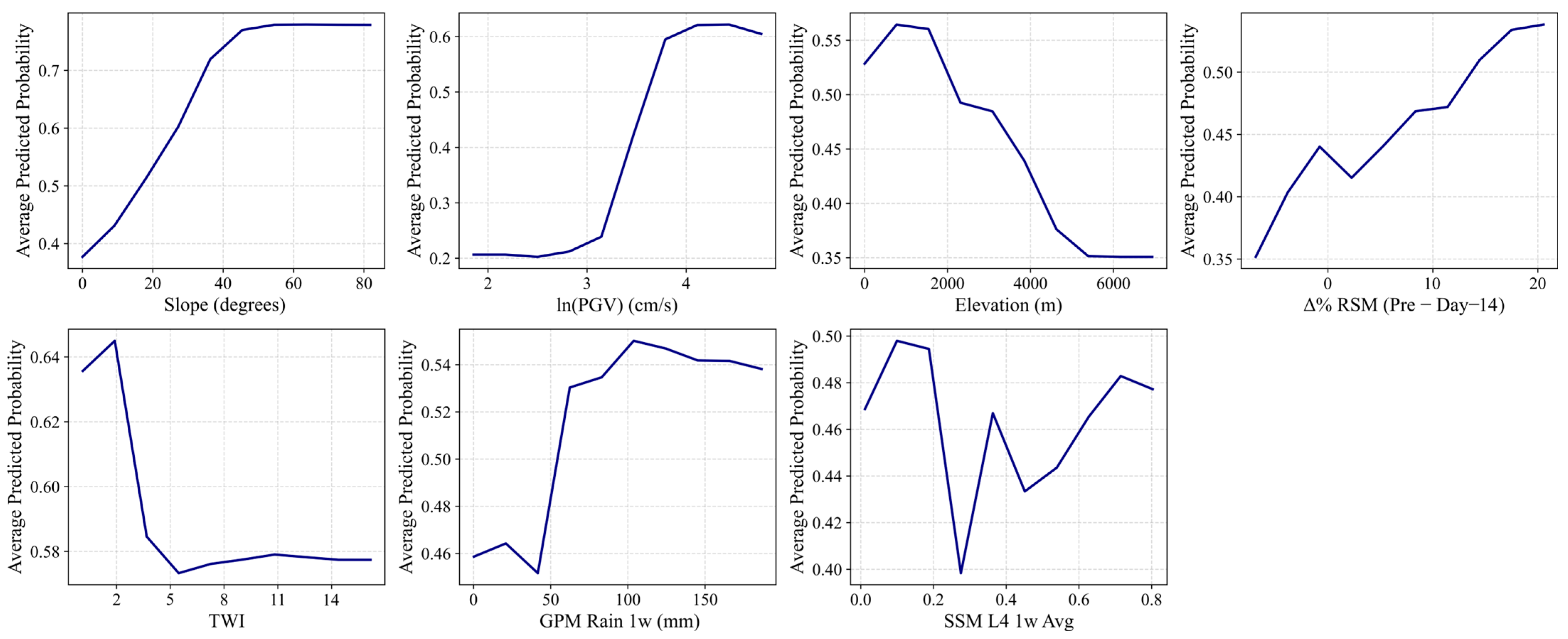
3.1. Data Exploration: Relationships Between Variables and Landslide Occurrence

Before developing the predictive model, exploratory data analysis was conducted to examine the relationships between landslide occurrence and the selected variables. This analysis aimed to provide initial insight into individual variable relevance as well as potential interactions that could influence landslide occurrence. Figure 6 presents a series of histograms that illustrate how landslide and non-landslide occurrences are distributed across binned intervals of key predictor variables. For each variable, the number of landslide (orange) and non-landslide (green) samples is shown per bin, accompanied by a series of black points connected by a dashed line, indicating the proportion of landslide cases in each bin. These univariate plots reveal important trends and threshold-like behaviors relevant to landslide susceptibility.

For PGV, the proportion of landslide cases increases noticeably with seismic intensity, particularly beyond approximately 20 cm/s (e.g., ln(PGV) > 3), reinforcing the expected influence of strong ground motion. Slope shows a similarly clear positive trend, with both the number and share of landslides increasing as terrain becomes steeper. In contrast, elevation exhibits an inverse pattern, where landslides are most frequent at lower altitudes. TWI displays a somewhat nonlinear relationship: landslides are more common in areas with lower TWI values, which often correspond to steep, convex, or well-drained slopes where water does not accumulate. These conditions may promote faster runoff and drier soils but still pose landslide risk due to slope instability or loose surface materials. These trends for PGV, slope, elevation, and TWI are consistent with previous seismic landslide studies [27,89], which reported similar associations between strong ground motion, steep terrain, and topographic controls on landslide occurrence.

Δ% RSM (Pre − Day–14), representing short-term changes in root zone soil moisture, shows a positive association with landslide share, particularly in bins with higher moisture change. GPM Rainfall over the one-week period prior to the earthquake also correlates with landslide occurrence, with the highest proportions observed in intermediate to high rainfall bins (~90–150 mm). Lastly, SSM L4 (1-week average) shows no clear monotonic relationship with landslide occurrence. This lack of a clear trend may reflect the multi-variable and context-dependent nature of landslide triggering, where soil moisture interacts with topographic and seismic factors in complex ways. Collectively, these results confirm the relevance of each selected variable and support the idea that both hydrological and geophysical factors contribute to slope failure. The trends also highlight the need for nonlinear and interaction-aware modeling approaches such as Random Forest.

Figure 7 also shows violin plots of the selected predictor variables, grouped by landslide and non-landslide cases of all five earthquakes together. Each violin combines a boxplot (showing median and interquartile range) with a rotated kernel density estimation plot that visualizes the distribution of values. The width of each shape reflects the relative frequency of data values—wider sections indicate more common values, while narrower regions reflect less frequent ones.

Overall, clear shifts in distribution are evident for PGV and slope, both of which have higher median values and broader spreads in landslide cases, consistent with their known role in triggering landslide. Elevation shows a lower median and tighter spread among landslide points, suggesting higher susceptibility at lower altitudes. Δ% RSM L4 (Pre − Day–14), GPM Rain 1w, and SSM L4 1w Ave also displays a higher median for landslide cases, indicating that recent increases in soil moisture may contribute to landslide.

Figure 8 presents bivariate heatmaps that illustrate how landslide occurrence varies with the combined influence of PGV and other conditioning variables. Each cell represents a bin combination, color-coded by the proportion of landslide cases (landslide share), with warmer tones indicating higher share of landslide cases. In most variable pairings, landslide share increases with PGV, particularly when combined with steep slopes, higher Δ% RSM L4 (Pre − Day–14), or elevated SSM L4 1w Ave, underscoring the amplifying effect of strong ground motion in conjunction with other predisposing factors. The interaction between PGV and slope, in particular, reveals the strongest concentration of high landslide share, highlighting the synergistic role of seismic shaking and terrain steepness. While variables such as TWI, GPM Rain 1w, and SSM L4 1w Ave did not exhibit clear or consistent trends in the univariate histograms (Figure 6), their interaction with PGV reveals areas of elevated landslide share—suggesting that their influence becomes more apparent under certain seismic or geomorphic conditions. These patterns highlight the nonlinear and context-dependent nature of landslide triggering, where the effect of a variable is shaped by its interaction with others.

These interaction maps emphasize the non-additive nature of landslide susceptibility and reinforce the need for multivariate modeling frameworks capable of capturing complex variable interplay. This supports the use of methods like Random Forest, which can model the joint behavior of contributing factors and account for their nonlinear interactions.

Figure 9 also presents bivariate heatmaps showing the proportion of landslide cases across combinations of slope and three hydrologically relevant variables: Δ% RSM L4 (Pre − Day–14), SSM L4 1w Ave, and GPM Rain 1w. In all three panels, steeper slopes consistently correspond to higher landslide share, confirming slope as a dominant predisposing factor. However, the role of hydrological variables becomes more apparent when viewed in combination with slope. For instance, elevated Δ% RSM L4 (Pre − Day–14) and higher SSM L4 1w Avg both amplify landslide share within each slope class, suggesting that short-term moisture buildup intensifies slope instability under steep terrain. Similarly, rainfall shows a compounding effect: higher rainfall bins are associated with increased landslide share, particularly at moderate and high slopes. These interaction patterns reinforce the idea that hydrological variables, while not always strongly predictive on their own, gain importance under topographic conditions favorable to failure.

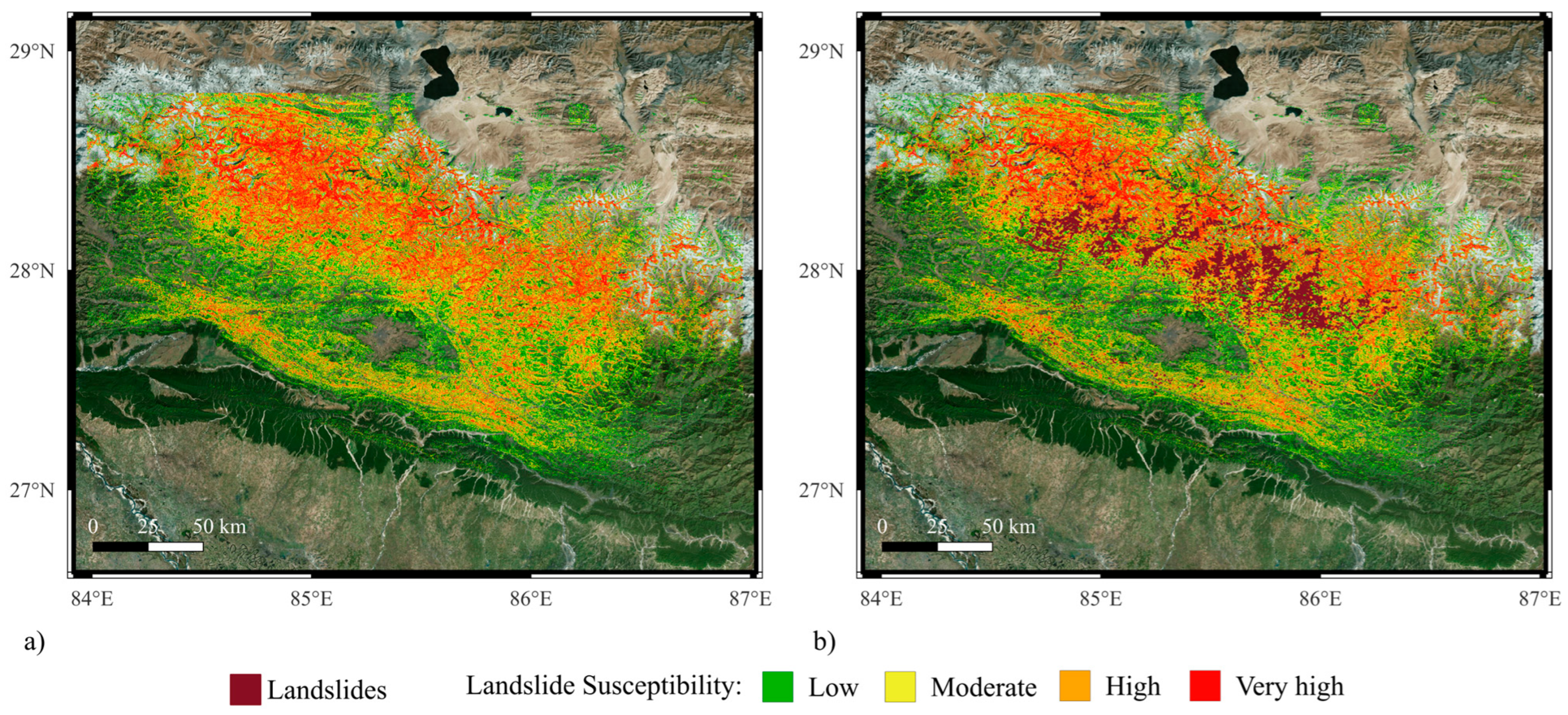
3.2. Landslide Model

After examining individual variables and their interactions, the Random Forest (RF) model was trained using the combined data from all five earthquake events—Nepal (2015), New Zealand (2016), Indonesia (2018), Papua New Guinea (2018), and Haiti (2021)—to evaluate landslide susceptibility in a unified modeling framework. A balanced 1:1 landslide to non-landslide (L/NL) ratio was maintained by downsampling each inventory to 4893 L and 4893 NL cases, ensuring equal contribution from all events. The model’s performance was evaluated on the test set, comprising 30% of the global dataset. As illustrated in the ROC curve (Figure 10), the model achieved an AUC of 0.95, demonstrating excellent discriminative power across probability thresholds. The confusion matrix at the default threshold of 0.5 (Figure 10) further reflects the model’s effectiveness: 6249 landslide cases (44.78% of the test set) and 6066 non-landslide cases (43.47%) were correctly predicted, while 900 non-landslide cases (6.45%) were incorrectly classified as landslides and 740 landslides (5.30%) were missed. Complementary evaluation metrics calculated on the test set show an accuracy of 88.25%, precision of 87.42%, recall of 89.39%, and an F1-score of 88.39%. These results emphasize the RF model’s ability to capture complex, nonlinear relationships among variables and its robust generalization across diverse geographic and seismic conditions.

To evaluate the reliability and uncertainty of the global landslide susceptibility model, a reliability diagram was generated (Figure 11). This plot compares the predicted probabilities of landslide occurrence to the actual observed frequencies. Each dot represents a bin of test samples with similar predicted probabilities, where the x-axis denotes the average predicted probability in that bin, and the y-axis indicates the observed proportion of landslides. Ideally, a well-calibrated model’s predictions should fall along the diagonal reference line, indicating that predicted probabilities closely match observed outcomes. In this study, the global model demonstrated strong calibration, with most points closely aligned with the diagonal and an Expected Calibration Error (ECE) of 0.04. Additionally, the Brier score was computed as 0.09, which reflects the mean squared difference between the predicted probabilities and the actual binary outcomes (0 for non-landslide, 1 for landslide). Lower Brier Scores indicate that the model’s probabilistic predictions are both accurate and confident. Together, the reliability curve, ECE, and Brier score suggest that the global model provides well-calibrated and reliable predictions for landslide occurrence.

To gain insight into the predictive contribution of each variable, Figure 12 presents permutation importance scores derived from the Random Forest model trained on the global dataset. These scores reflect the mean decrease in AUC when each variable is randomly shuffled, indicating how much each feature contributes to the model’s ability to distinguish landslide from non-landslide cases. PGV and Slope emerge as the most influential predictors, consistent with their strong physical roles in seismic landslide triggering. SSM L4 1w Avg and Δ% RSM (Pre − Day–14) also show notable contributions, emphasizing the value of integrating SMAP-derived soil moisture signals. In contrast, TWI, GPM Rain 1w, and LC have relatively lower importance, possibly due to redundancy with stronger predictors or limited variability across events. The higher importance of SMAP-derived variables over GPM rainfall and TWI likely reflects their ability to represent the cumulative and antecedent hydrologic state of the soil—an essential preconditioning factor in seismic landslides. Unlike rainfall data, which capture only recent precipitation input, SMAP soil moisture integrates effects of infiltration, retention, and drainage, making it a more direct proxy for the subsurface conditions that influence slope stability under shaking. Overall, the ranking underscores the complex interplay between ground shaking, terrain, and hydrologic conditions in controlling landslide susceptibility.

To better understand how each input variable influences the predicted probability of landslide occurrence, Partial Dependence Plots (PDPs) [65,138,139] were used. A PDP illustrates the relationship between a single variable and the model’s predicted probability, while all other variables are held constant. This allows us to evaluate how sensitive the model’s predictions are to changes in that specific variable. In essence, PDPs provide a visual form of sensitivity analysis, helping us determine whether increasing or decreasing a particular feature significantly shifts the landslide probability predicted by the model. For instance, to generate a PDP for slope, the slope value in all landslide and non-landslide observations is replaced with a fixed value (e.g., 20 degrees), while all other variables remain unchanged. The developed Random Forest model is then used to compute the predicted probabilities across all modified observations, and the results are averaged. Repeating this process across a range of slope values yields a plot that reflects how the average predicted landslide probability varies with slope. This process is applied to each variable of interest, offering intuitive insights into the independent contribution and influence of each feature on landslide susceptibility.

Figure 13 presents PDPs illustrating the isolated influence of each input feature on the predicted probability of landslide occurrence. These plots quantify the average model response when a single variable changes across its range, while all other features remain fixed. Several distinct patterns emerge. The PDP for slope shows a strong positive influence, with predicted landslide probability rising steadily from approximately 40% to over 75% as slope increases. This trend exhibits a saturation effect, where the probability climbs rapidly up to around 40°, beyond which further increases in slope yield minimal additional impact. Moreover, a similar saturation pattern is observed in both TWI and GPM Rain (1w), though in opposite directions: as rainfall increases, the predicted probability goes up at first and then stays roughly the same; in contrast, higher TWI values cause the probability to drop quickly and then remain steady. The PGV plot indicates a threshold effect. At low PGV values, the predicted probability remains low, but once a critical level is exceeded (around ln(PGV) ≈ 3.2), the probability increases sharply, suggesting the presence of a triggering threshold for landslide occurrence. The upward trend in Δ% RSM (Pre − Day–14) highlights the role of antecedent moisture buildup. An increase in root-zone soil moisture in the two weeks before the event can raise the predicted landslide probability by more than 20 percentage points, underscoring the importance of pre-event moisture buildup. For SSM L4 1w Avg, the model exhibits a U-shaped response, where both low and high soil moisture conditions correspond to increased landslide probability. This may reflect different failure mechanisms under dry versus saturated conditions. Together, these plots function as sensitivity analysis, offering interpretable insights into how strongly and in what direction each factor influences the model’s output.

4. Discussion

To further evaluate the model’s generalizability across diverse seismic, geotechnical, and hydrological settings, a leave-one-earthquake-out cross-validation strategy was implemented. In this phase, the Random Forest model was trained using landslide and non-landslide data from four of the five earthquake inventories and then tested on the held-out fifth event. This approach simulates real-world prediction scenarios, where models must be applied to new earthquake events without using local landslide data for training, and ensures that model performance reflects true spatial transferability.

To benchmark the performance of the proposed model, results were compared against the USGS global landslide hazard model developed by Nowicki Jessee et al. [27]. Their logistic regression model, trained on 23 global inventories, incorporates geospatial variables such as slope, PGV, lithology, land cover, and compound topographic index (CTI) to produce hazard maps at approximately 250 m resolution. The publicly available USGS landslide hazard map rasters [140] represent areal probabilities of landslide occurrence—that is, the expected fraction of each grid cell affected by landsliding—obtained through a nonlinear transformation applied to the original logistic regression outputs, as described in Nowicki Jessee et al. [27]. For consistency in evaluation, the inverse of this transformation was applied to recover the original probabilistic outputs, allowing a direct comparison between the two models.

For each held-out event, model evaluation is presented using two complementary figures: (1) the ROC curve and confusion matrix derived from this method’s predictions on the held-out event, along with the ROC curve of the USGS model for comparison; and (2) the corresponding landslide probability map generated without including that event’s inventory in the training process.

Specifically, the results are presented as follows: Haiti 2021 in Figure 14 and Figure 15; Indonesia 2018 in Figure 16 and Figure 17; Papua New Guinea 2018 in Figure 18 and Figure 19; New Zealand 2016 in Figure 20 and Figure 21; and Nepal 2015 in Figure 22 and Figure 23. The susceptibility in the landslide hazard probability maps was classified into four classes: low (0.2–0.4), moderate (0.4–0.6), high (0.6–0.8), and very high (0.8–1.0) [89].

For generating the landslide probability maps, a regular grid based on the resolution of the slope raster was used. All other variables were interpolated to this grid (via bilinear interpolation), enabling spatially continuous and coherent probability predictions.

Table 4. Summary of evaluation metrics for each leave-one-earthquake-out test case.

Left-Out Landslide Inventory	AUC	Accuracy	Precision	Recall	F1-Score
Nippes, Haiti 2021	0.84	0.75	0.72	0.83	0.77
Palu, Indonesia 2018	0.83	0.77	0.78	0.76	0.77
Tari, Papua New Guinea 2018	0.89	0.81	0.83	0.76	0.80
Kaikoura, New Zealand 2016	0.89	0.80	0.84	0.75	0.79
Gorkha, Nepal 2015	0.84	0.70	0.63	0.95	0.76
Average in this study	0.86	0.76	0.76	0.81	0.78

summarizes the performance metrics for each earthquake inventory under the leave-one-earthquake-out cross-validation framework. Across all five test cases, the model maintained robust predictive ability, with AUC values ranging from 0.83 to 0.89 and F1-scores from 0.76 to 0.80. Notably, the model achieved high recall for most events, indicating strong sensitivity to true landslide occurrences. Although precision varied slightly across inventories, the model consistently balanced accuracy and generalization. On average, the Random Forest model achieved an AUC of 0.86, accuracy of 0.76, precision of 0.76, recall of 0.81, and an F1-score of 0.78 across the five leave-out tests.

These average values for leave-one-earthquake-out test cases exceed those reported in previous studies using similar approaches with commonly used variables (PGV, Slope, TWI, and Landcover data), such as Nowicki Jessee et al. [27] and He et al. [89], underscoring the improved predictive performance achieved through the integration of soil moisture variables in this study. For example, Figure 24 compares the average evaluation metrics from our leave-one-earthquake-out tests with those reported by He et al. [89], who applied a similar Random Forest approach using nine common geospatial variables (including MMI, slope, elevation, lithology, and TWI), but without incorporating soil moisture information. While the inventories used in their study differ from ours, this comparison highlights the improved model performance achieved through the integration of SMAP-derived soil moisture indicators. Across all five metrics—AUC, Accuracy, Precision, Recall, and F1-score—our model demonstrates higher average values, reinforcing the value of including antecedent hydrologic conditions in seismic landslide prediction.

The uncertainty and reliability were also assessed using reliability diagrams and Brier scores for each leave-one-earthquake-out test case (Figure 25). The models generally demonstrate moderate calibration, with some variation across events. The calibration curves illustrate event-specific patterns: The leave-Nepal-out case shows notable overestimation across most probability bins (ECE = 0.24), while New Zealand 2016 tends to underestimate landslide probabilities (ECE = 0.14). In contrast, Indonesia 2018 (ECE = 0.03), Papua New Guinea 2018 (ECE = 0.07), and Haiti 2021 (ECE = 0.06) display closer alignment with the ideal calibration line. The Brier scores, which assess overall probabilistic accuracy, range from 0.16 (Indonesia 2018) to 0.19 (New Zealand 2016), with an average of 0.18 across all events. Since Brier scores below 0.2 are generally considered indicative of good performance, these values suggest that the predicted probabilities remain reasonably accurate, despite some calibration deviations.

Despite the advances presented in this study, several considerations remain that warrant further investigation in future research. While this study focuses on earthquake-induced landslides, it is important to acknowledge that remote sensing–derived inventories—due to their limited temporal resolution—may include some landslides triggered or influenced by rainfall. Such overlaps are common in co-seismic inventories and reflect the complex interplay between seismic shaking and hydrologic conditions. By incorporating both rainfall and soil moisture data into the modeling framework, this study accounts for these interactions more comprehensively than previous models [27,89]. Additionally, the spatial resolution of SMAP soil moisture data (e.g., 9 km) may reduce prediction accuracy. While data exploration in Section 3.1 and the feature importance analysis indicate that satellite-based soil moisture from SMAP offers informative value for modeling earthquake-induced landslides, its relatively coarse spatial resolution is acknowledged. Future work should explore higher-resolution datasets—such as SMAP–Sentinel fused products (1 km), downscaled soil moisture models, or data from next-generation missions like NASA–ISRO SAR (NISAR) [141]—to improve spatial precision.

Another limitation is the landslide inventories used in this study, primarily derived from remote sensing, without consistent classification by failure type (e.g., shallow slides, deep-seated landslides, debris flows). As a result, our model does not differentiate between failure mechanisms. This is a common approach in large-scale studies [27,89], but it is important to note that different landslide types exhibit distinct instability mechanisms. For example, shallow slides and debris flows are strongly influenced by near-surface soil moisture, while deep-seated landslides—rare in this research inventories based on available reports—are driven more by long-term hydrological conditions and subsurface structure [142,143]. Given the dominance of shallow failures in our datasets, soil moisture plays a critical role in both preconditioning and amplifying seismic response. This emphasizes the need for future models to incorporate failure-type-specific mechanisms when inventories with such detail become available.

Moreover, the current model focuses on large-magnitude earthquakes; expanding the dataset to include lower-magnitude events or region-specific inventories could enhance the model’s generalizability and reveal more nuanced insights into the role of soil moisture. Lastly, the influence of post-earthquake soil moisture and rainfall data on delayed landslide failures remains an open question. Future studies should examine this interplay in more detail, ideally using higher-frequency precipitation and soil moisture data to better capture hydrologic changes following seismic events.

5. Conclusions

This study developed a global Random Forest (RF) model to assess earthquake-induced landslide susceptibility by integrating NASA’s SMAP-derived soil moisture products with common seismic and geospatial variables. Based on five major earthquake inventories, the following key conclusions can be drawn:

• Soil moisture improves model performance: Incorporating SMAP-derived surface and root-zone soil moisture indicators enhanced landslide prediction. Short-term indicators such as SSM L4 1w Avg and Δ% RSM (Pre − Day–14) ranked among the top predictors, reflecting the importance of hydrologic preconditioning in co-seismic slope failures.
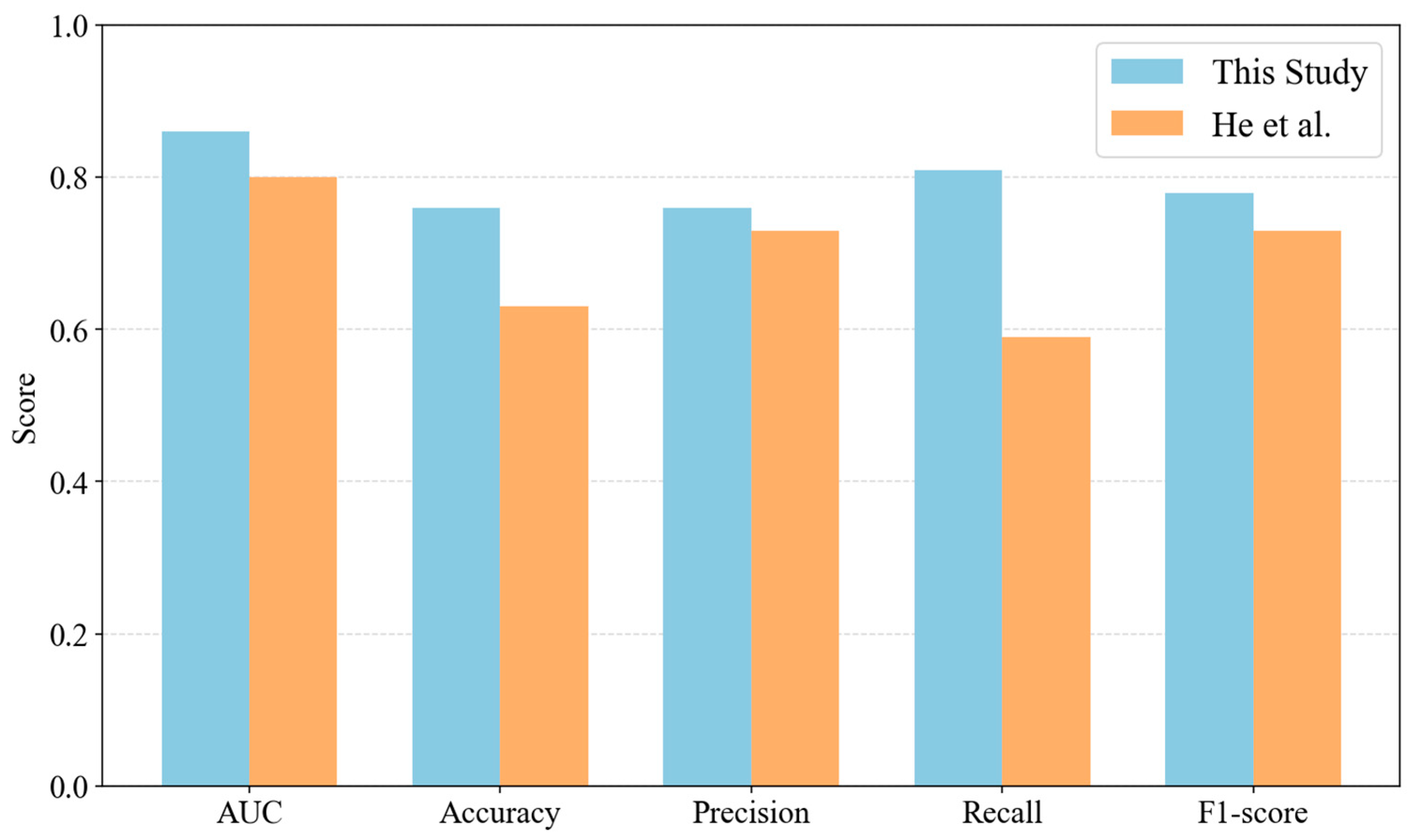
• High predictive accuracy achieved: The leave-one-earthquake-out cross-validation yielded strong performance (average AUC = 0.86, F1-score = 0.78, and accuracy = 0.83), consistently outperforming the United States Geological Survey (USGS) landslide model and another well-established global Random Forest model that did not consider soil moisture.
• Dynamic variables outperform static proxies: The use of time-varying satellite-based soil moisture and rainfall (e.g., GPM) provided better insights than static proxies like TWI. This supports the transition from static to dynamic modeling in future hazard frameworks.
• Transferability demonstrated: The model showed generalizability across five diverse earthquake events in different climatic and geological settings, indicating its potential for near-real-time application in global earthquake impacts assessments.

While this study advances seismic landslide modeling by integrating dynamic satellite-based hydrologic variables, there are opportunities for future studies to further enhance the framework. These include using higher-resolution soil moisture products to improve spatial precision, incorporating landslide inventories with failure type classifications to support mechanism-specific modeling, and expanding the dataset to include lower-magnitude or region-specific events to improve generalizability. Additionally, future work could explore the influence of post-earthquake soil moisture and rainfall data on delayed landslide failures using higher-frequency hydrologic data.

References

1. Froude, M.J.; Petley, D.N. Global Fatal Landslide Occurrence from 2004 to 2016. Nat. Hazards Earth Syst. Sci. 2018, 18, 2161–2181. [Google Scholar] [CrossRef]
2. Keefer, D.K. Investigating Landslides Caused by Earthquakes—A Historical Review. Surv. Geophys. 2002, 23, 473–510. [Google Scholar] [CrossRef]
3. Santangelo, N.; Forte, G.; Falco, M.; Chirico, G.B.; Santo, A. New Insights on Rainfall Triggering Flow-like Landslides and Flash Floods in Campania (Southern Italy). Landslides 2021, 18, 2923–2933. [Google Scholar] [CrossRef]
4. Liu, P.; Wei, Y.; Wang, Q.; Chen, Y.; Xie, J. Research on Post-Earthquake Landslide Extraction Algorithm Based on Improved U-Net Model. Remote Sens. 2020, 12, 894. [Google Scholar] [CrossRef]
5. Kalantar, B.; Ueda, N.; Saeidi, V.; Ahmadi, K.; Halin, A.A.; Shabani, F. Landslide Susceptibility Mapping: Machine and Ensemble Learning Based on Remote Sensing Big Data. Remote Sens. 2020, 12, 1737. [Google Scholar] [CrossRef]
6. Bird, J.F.; Bommer, J.J. Earthquake Losses Due to Ground Failure. Eng. Geol. 2004, 75, 147–179. [Google Scholar] [CrossRef]
7. Fan, X.; Scaringi, G.; Korup, O.; West, A.J.; Westen, C.J.; Tanyas, H.; Huang, R. Earthquake-induced Chains of Geologic Hazards: Patterns, Mechanisms, and Impacts. Rev. Geophys. 2019, 57, 421–503. [Google Scholar] [CrossRef]
8. Allstadt, K.E.; Thompson, E.M.; Hearne, M.; Jessee, M.N.; Zhu, J.; Wald, D.J.; Tanyas, H. Integrating Landslide and Liquefaction Hazard and Loss Estimates with Existing USGS Real-time Earthquake Information Products. In Proceedings of the 16th World Conference on Earthquake Engineering, Santiago, Chile, 9–13 January 2017. [Google Scholar]
9. Daniell, J.E.; Schaefer, A.M.; Wenzel, F. Losses Associated with Secondary Effects in Earthquakes. Front. Built Environ. 2017, 3, 30. [Google Scholar] [CrossRef]
10. Marano, K.D.; Wald, D.J.; Allen, T.I. Global Earthquake Casualties Due to Secondary Effects: A Quantitative Analysis for Improving Rapid Loss Analyses. Nat. Hazards 2010, 52, 319–328. [Google Scholar] [CrossRef]
11. Gautam, D. Unearthed Lessons of 25 April 2015 Gorkha Earthquake (MW 7.8): Geotechnical Earthquake Engineering Perspectives. Geomat. Nat. Hazards Risk 2017, 8, 1358–1382. [Google Scholar] [CrossRef]
12. Xu, C.; Xu, X.; Yao, X.; Dai, F. Three (Nearly) Complete Inventories of Landslides Triggered by the May 12, 2008 Wenchuan Mw 7.9 Earthquake of China and Their Spatial Distribution Statistical Analysis. Landslides 2014, 11, 441–461. [Google Scholar] [CrossRef]
13. Dai, F.C.; Xu, C.; Yao, X.; Xu, L.; Tu, X.B.; Gong, Q.M. Spatial Distribution of Landslides Triggered by the 2008 Ms 8.0 Wenchuan Earthquake, China. J. Asian Earth Sci. 2011, 40, 883–895. [Google Scholar] [CrossRef]
14. Roback, K.; Clark, M.K.; West, A.J.; Zekkos, D.; Li, G.; Gallen, S.F.; Godt, J.W. The Size, Distribution, and Mobility of Landslides Caused by the 2015 Mw 7.8 Gorkha Earthquake, Nepal. Geomorphology 2018, 301, 121–138. [Google Scholar] [CrossRef]
15. Hashash, Y.; Tiwari, B.; Moss, R.E.; Asimaki, D.; Clahan, K.B.; Kieffer, D.S.; Adhikari, B. Geotechnical Field Reconnaissance: Gorkha (Nepal) Earthquake of April 25 2015. Available online: https://www.geerassociation.org/components/com_geer_reports/geerfiles/Nepal_GEER_Report_V1_15.pdf (accessed on 10 July 2025).
16. Kargel, J.S.; Leonard, G.J.; Shugar, D.H.; Haritashya, U.K.; Bevington, A.; Fielding, E.J.; Young, N. Geomorphic and Geologic Controls of Geohazards Induced by Nepal’s 2015 Gorkha Earthquake. Science 2016, 351, 8353. [Google Scholar] [CrossRef]
17. Zhao, B. Landslides Triggered by the 2018 Mw 7.5 Palu Supershear Earthquake in Indonesia. Eng. Geol. 2021, 294, 106406. [Google Scholar] [CrossRef]
18. Mason, H.B.; Gallant, A.P.; Hutabarat, D.; Montgomery, J.; Reed, A.N.; Wartman, J.; Hanifa, R. Geotechnical Reconnaissance: The 28 September 2018 M7.5 Palu-donggala, Indonesia Earthquake. 2021. Available online: https://www.geerassociation.org/?view=geerreports&id=88&layout=default (accessed on 10 July 2025).
19. Natawidjaja, D.H.; Daryono, M.R.; Prasetya, G.; Liu, P.L.; Hananto, N.D.; Kongko, W.; Tawil, S. The 2018 MW 7.5 Palu ‘Supershear’Earthquake Ruptures Geological Fault’s Multisegment Separated by Large Bends: Results from Integrating Field Measurements, LiDAR, Swath Bathymetry and Seismic-Reflection Data. Geophys. J. Int. 2021, 224, 985–1002. [Google Scholar]
20. Tang, C.; Westen, C.J.V.; Tanyaş, H.; Jetten, V.G. Analyzing Post-Earthquake Landslide Activity Using Multi-Temporal Landslide Inventories near the Epicentral Area of the 2008 Wenchuan Earthquake. Nat. Hazards Earth Syst. Sci. 2016, 16, 2641–2655. [Google Scholar] [CrossRef]
21. Jibson, R.W.; Harp, E.L.; Michael, J.A. A method for producing digital probabilistic seismic landslide hazard maps. Eng. Geol. 2000, 58, 271–289. [Google Scholar] [CrossRef]
22. Yunus, A.P.; Fan, X.; Tang, X.; Jie, D.; Xu, Q.; Huang, R. Decadal Vegetation Succession from MODIS Reveals the Spatio-Temporal Evolution of Post-Seismic Landsliding after the 2008 Wenchuan Earthquake. Remote Sens. Environ. 2020, 236, 111476. [Google Scholar] [CrossRef]
23. Hovius, N.; Meunier, P.; Lin, C.W.; Chen, H.; Chen, Y.G.; Dadson, S.; Lines, M. Prolonged Seismically Induced Erosion and the Mass Balance of a Large Earthquake. Earth Planet. Sci. Lett. 2011, 304, 347–355. [Google Scholar] [CrossRef]
24. Dadson, S.J.; Hovius, N.; Chen, H.; Dade, W.B.; Lin, J.C.; Hsu, M.L.; Stark, C.P. Earthquake-Triggered Increase in Sediment Delivery from an Active Mountain Belt. Geology 2004, 32, 733–736. [Google Scholar] [CrossRef]
25. Wasowski, J.; Keefer, D.K.; Lee, C.T. Toward the next Generation of Research on Earthquake-Induced Landslides: Current Issues and Future Challenges. Eng. Geol. 2011, 122, 1–8. [Google Scholar] [CrossRef]
26. Robinson, T.R.; Rosser, N.J.; Davies, T.R.; Wilson, T.M.; Orchiston, C. Near-real-time Modeling of Landslide Impacts to Inform Rapid Response: An Example from the 2016 Kaikōura, New Zealand, Earthquake. Bull. Seismol. Soc. Am. 2018, 108, 1665–1682. [Google Scholar] [CrossRef]
27. Nowicki Jessee, M.A.; Hamburger, M.W.; Allstadt, K.; Wald, D.J.; Robeson, S.M.; Tanyas, H.; Thompson, E.M. A Global Empirical Model for Near-real-time Assessment of Seismically Induced Landslides. J. Geophys. Res. Earth Surf. 2018, 123, 1835–1859. [Google Scholar] [CrossRef]
28. Shao, X.; Xu, C. Earthquake-Induced Landslides Susceptibility Assessment: A Review of the State-of-the-Art. Nat. Hazards Res. 2022, 2, 172–182. [Google Scholar] [CrossRef]
29. Wang, X.; Wang, X.; Zhang, X.; Wang, L.; Guo, H.; Li, D. Near Real-Time Spatial Prediction of Earthquake-Induced Landslides: A Novel Interpretable Self-Supervised Learning Method. Int. J. Digit. Earth 2023, 16, 1885–1906. [Google Scholar] [CrossRef]
30. Cheng, Q.; Tian, Y.; Lu, X.; Huang, Y.; Ye, L. Near-Real-Time Prompt Assessment for Regional Earthquake-Induced Landslides Using Recorded Ground Motions. Comput. Geosci. 2021, 149, 104709. [Google Scholar] [CrossRef]
31. Alvioli, M.; Poggi, V.; Peresan, A.; Scaini, C.; Tamaro, A.; Guzzetti, F. A Scenario-Based Approach for Immediate Post-Earthquake Rockfall Impact Assessment. Landslides 2024, 21, 1–16. [Google Scholar] [CrossRef]
32. Reichenbach, P.; Rossi, M.; Malamud, B.D.; Mihir, M.; Guzzetti, F. A Review of Statistically-Based Landslide Susceptibility Models. Earth-Sci. Rev. 2018, 180, 60–91. [Google Scholar] [CrossRef]
33. Jibson, R.W. Methods for Assessing the Stability of Slopes during Earthquakes—A Retrospective. Eng. Geol. 2011, 122, 43–50. [Google Scholar] [CrossRef]
34. Zhang, A.; Wang, X.; Pedrycz, W.; Yang, Q.; Wang, X.; Guo, H. Near Real-Time Spatial Prediction of Earthquake-Triggered Landslides Based on Global Inventories from 2008 to 2022. Soil Dyn. Earthq. Eng. 2024, 185, 108890. [Google Scholar] [CrossRef]
35. Ji, J.; Zhang, W.; Zhang, F.; Gao, Y.; Lü, Q. Reliability Analysis on Permanent Displacement of Earth Slopes Using the Simplified Bishop Method. Comput. Geotech. 2020, 117, 103286. [Google Scholar] [CrossRef]
36. Valagussa, A.; Frattini, P.; Crosta, G.B. Earthquake-induced rockfall hazard zoning. Eng. Geol. 2014, 182, 213–225. [Google Scholar] [CrossRef]
37. Bray, J.D.; Travasarou, T. Simplified Procedure for Estimating Earthquake-Induced Deviatoric Slope Displacements. J. Geotech. Geoenviron. Eng. 2007, 133, 381–392. [Google Scholar] [CrossRef]
38. Gallen, S.F.; Clark, M.K.; Godt, J.W.; Roback, K.; Niemi, N.A. Application and Evaluation of a Rapid Response Earthquake-Triggered Landslide Model to the 25 April 2015 Mw 7.8 Gorkha Earthquake, Nepal. Tectonophysics 2017, 714, 173–187. [Google Scholar] [CrossRef]
39. Dreyfus, D.; Rathje, E.M.; Jibson, R.W. The Influence of Different Simplified Sliding-Block Models and Input Parameters on Regional Predictions of Seismic Landslides Triggered by the Northridge Earthquake. Eng. Geol. 2013, 163, 41–54. [Google Scholar] [CrossRef]
40. Godt, J.; Sener, B.; Verdin, K.L.; Wald, D.J.; Earle, P.S.; Harp, E.L.; Jibson, R. Rapid Assessment of Earthquake-Induced Landsliding. In Proceedings of the First World Landslide Forum, Tokyo, Japan, 18–21 November 2008; United Nations University: Tokyo, Japan; Volume 4, pp. 219–222. [Google Scholar]
41. Huang, D.; Wang, G.; Du, C.; Jin, F.; Feng, K.; Chen, Z. An Integrated SEM-Newmark Model for Physics-Based Regional Coseismic Landslide Assessment. Soil Dyn. Earthq. Eng. 2020, 132, 106066. [Google Scholar] [CrossRef]
42. Lima, P.; Steger, S.; Glade, T.; Murillo-García, F.G. Literature Review and Bibliometric Analysis on Data-Driven Assessment of Landslide Susceptibility. J. Mt. Sci. 2022, 19, 1670–1698. [Google Scholar] [CrossRef]
43. Anbalagan, R. Landslide Hazard Evaluation and Zonation Mapping in Mountainous Terrain. Eng. Geol. 1992, 32, 269–277. [Google Scholar] [CrossRef]
44. Pandey, A.; Dabral, P.P.; Chowdary, V.M.; Yadav, N.K. Landslide hazard zonation using remote sensing and GIS: A case study of Dikrong river basin, Arunachal Pradesh, India. Environ. Geol. 2008, 54, 1517–1529. [Google Scholar] [CrossRef]
45. Kouli, M.; Loupasakis, C.; Soupios, P.; Vallianatos, F. Landslide hazard zonation in high risk areas of Rethymno Prefecture, Crete Island, Greece. Nat. Hazards 2010, 52, 599–621. [Google Scholar] [CrossRef]
46. Guzzetti, F.; Carrara, A.; Cardinali, M.; Reichenbach, P. Landslide Hazard Evaluation: A Review of Current Techniques and Their Application in a Multi-Scale Study, Central Italy. Geomorphology 1999, 31, 181–216. [Google Scholar] [CrossRef]
47. Nadim, F.; Kjekstad, O.; Peduzzi, P.; Herold, C.; Jaedicke, C. Global landslide and avalanche hotspots. Landslides 2006, 3, 159–173. [Google Scholar] [CrossRef]
48. Shano, L.; Raghuvanshi, T.K.; Meten, M. Landslide Susceptibility Evaluation and Hazard Zonation Techniques—A Review. Geoenviron. Disasters 2020, 7, 18. [Google Scholar] [CrossRef]
49. Carrara, A.; Cardinali, M.; Guzzetti, F.; Reichenbach, P. GIS technology in mapping landslide hazard. In Geographical Information Systems in Assessing Natural Hazards; Springer: Dordrecht, The Netherlands, 1995; pp. 135–175. [Google Scholar]
50. Lee, C.T.; Huang, C.C.; Lee, J.F.; Pan, K.L.; Lin, M.L.; Dong, J.J. Statistical Approach to Earthquake-Induced Landslide Susceptibility. Eng. Geol. 2008, 100, 43–58. [Google Scholar] [CrossRef]
51. Farahani, A.; Ghayoomi, M. Soil moisture-based global liquefaction model (SMGLM) using soil moisture active passive (SMAP) satellite data. Soil Dyn. Earthq. Eng. 2024, 177, 108350. [Google Scholar] [CrossRef]
52. Nowicki, M.A.; Wald, D.J.; Hamburger, M.W.; Hearne, M.; Thompson, E.M. Development of a Globally Applicable Model for near Real-Time Prediction of Seismically Induced Landslides. Eng. Geol. 2014, 173, 54–65. [Google Scholar] [CrossRef]
53. Farahani, A.; Ghayoomi, M. Updates to a Soil Moisture-Based Global Liquefaction Model. Jpn. Geotech. Soc. Spec. Publ. 2024, 10, 860–865. [Google Scholar] [CrossRef]
54. Umar, Z.; Pradhan, B.; Ahmad, A.; Jebur, M.N.; Tehrany, M.S. Earthquake Induced Landslide Susceptibility Mapping Using an Integrated Ensemble Frequency Ratio and Logistic Regression Models in West Sumatera Province, Indonesia. Catena 2014, 118, 124–135. [Google Scholar] [CrossRef]
55. Batar, A.K.; Watanabe, T. Landslide Susceptibility Mapping and Assessment Using Geospatial Platforms and Weights of Evidence (WoE) Method in the Indian Himalayan Region: Recent Developments, Gaps, and Future Directions. ISPRS Int. J. Geo-Inf. 2021, 10, 114. [Google Scholar] [CrossRef]
56. Kritikos, T.; Robinson, T.R.; Davies, T.R. Regional Coseismic Landslide Hazard Assessment without Historical Landslide Inventories: A New Approach. J. Geophys. Res. Earth Surf. 2015, 120, 711–729. [Google Scholar] [CrossRef]
57. Parker, R.N.; Rosser, N.J.; Hales, T.C. Spatial Prediction of Earthquake-Induced Landslide Probability. Nat. Hazards Earth Syst. Sci. Discuss. 2017, 2017, 1–29. [Google Scholar]
58. Farahani, A.; Moradikhaneghahi, M.; Ghayoomi, M.; Jacobs, J.M. Application of soil moisture active passive (SMAP) satellite data in seismic response assessment. Remote Sens. 2022, 14, 4375. [Google Scholar] [CrossRef]
59. Ghayoomi, M.; Farahani, A. Soil Moisture From Space. GeoStrata Mag. Arch. 2025, 29, 30–38. [Google Scholar] [CrossRef]
60. Farahani, A.; Ghayoomi, M. Assessing Correlations between SAR-Based Damage Proxy Maps and Geospatial Variables for Enhanced Earthquake Damage Analysis. In Proceedings of the Geotechnical Frontiers 2025, Louisville, Kentucky, 2–5 March 2025; pp. 328–336. Available online: https://ascelibrary.org/doi/abs/10.1061/9780784485989.033 (accessed on 10 July 2025).
61. Sun, D.; Chen, D.; Zhang, J.; Mi, C.; Gu, Q.; Wen, H. Landslide Susceptibility Mapping Based on Interpretable Machine Learning from the Perspective of Geomorphological Differentiation. Land 2023, 12, 1018. [Google Scholar] [CrossRef]
62. Ma, S.; Shao, X.; Xu, C. Estimating the Quality of the Most Popular Machine Learning Algorithms for Landslide Susceptibility Mapping in 2018 Mw 7.5 Palu Earthquake. Remote Sens. 2023, 15, 4733. [Google Scholar] [CrossRef]
63. Xiao, S.; Xiao, T.; Jiang, R.; Wang, H.; Ju, L.; Zhang, L. Two-Phase Strategy for Rapid and Unbiased Assessment of Earthquake-Induced Landslides. Eng. Geol. 2024, 336, 107562. [Google Scholar] [CrossRef]
64. Farahani, A.; Ghayoomi, M.; Jacobs, J.M. The Use of SMAP to Investigate the Application of Remotely Sensed Soil Moisture Data in Earthquake Impacts Assessment. In Proceedings of the AGU Fall Meeting Abstracts, San Francisco, CA, USA, 11–15 December 2023; Volume 2023, p. H13M-1639. [Google Scholar]
65. Das, R.; Tien, P.V.; Wegmann, K.W.; Chakraborty, M. Machine Learning-Based Assessment of Regional-Scale Variation of Landslide Susceptibility in Central Vietnam. PLoS ONE 2024, 19, e0308494. [Google Scholar] [CrossRef] [PubMed]
66. Regmi, A.D.; Dhital, M.R.; Zhang, J.Q.; Su, L.J.; Chen, X.Q. Landslide Susceptibility Assessment of the Region Affected by the 25 April 2015 Gorkha Earthquake of Nepal. J. Mt. Sci. 2016, 13, 1941–1957. [Google Scholar] [CrossRef]
67. Pyakurel, A.; Dahal, B.K.; Gautam, D. Does Machine Learning Adequately Predict Earthquake Induced Landslides? Soil Dyn. Earthq. Eng. 2023, 171, 107994. [Google Scholar] [CrossRef]
68. Zhang, W.; Li, H.; Han, L.; Chen, L.; Wang, L. Slope Stability Prediction Using Ensemble Learning Techniques: A Case Study in Yunyang County, Chongqing, China. J. Rock Mech. Geotech. Eng. 2022, 14, 1089–1099. [Google Scholar] [CrossRef]
69. Dou, J.; Yunus, A.P.; Bui, D.T.; Merghadi, A.; Sahana, M.; Zhu, Z.; Pham, B.T. Improved Landslide Assessment Using Support Vector Machine with Bagging, Boosting, and Stacking Ensemble Machine Learning Framework in a Mountainous Watershed, Japan. Landslides 2020, 17, 641–658. [Google Scholar] [CrossRef]
70. Chang, Z.; Du, Z.; Zhang, F.; Huang, F.; Chen, J.; Li, W.; Guo, Z. Landslide Susceptibility Prediction Based on Remote Sensing Images and GIS: Comparisons of Supervised and Unsupervised Machine Learning Models. Remote Sens. 2020, 12, 502. [Google Scholar] [CrossRef]
71. Karakas, G.; Unal, E.O.; Cetinkaya, S.; Ozcan, N.T.; Karakas, V.E.; Can, R.; Kocaman, S. Analysis of Landslide Susceptibility Prediction Accuracy with an Event-Based Inventory: The 6 February 2023 Turkiye Earthquakes. Soil Dyn. Earthq. Eng. 2024, 178, 108491. [Google Scholar] [CrossRef]
72. Lary, D.J.; Alavi, A.H.; Gandomi, A.H.; Walker, A.L. Machine Learning in Geosciences and Remote Sensing. Geosci. Front. 2016, 7, 3–10. [Google Scholar] [CrossRef]
73. Merghadi, A.; Yunus, A.P.; Dou, J.; Whiteley, J.; ThaiPham, B.; Bui, D.T.; Abderrahmane, B. Machine Learning Methods for Landslide Susceptibility Studies: A Comparative Overview of Algorithm Performance. Earth-Sci. Rev. 2020, 207, 103225. [Google Scholar] [CrossRef]
74. Dahal, A.; Lombardo, L. Explainable Artificial Intelligence in Geoscience: A Glimpse into the Future of Landslide Susceptibility Modeling. Comput. Geosci. 2023, 176, 105364. [Google Scholar] [CrossRef]
75. Hong, H.; Shahabi, H.; Shirzadi, A.; Chen, W.; Chapi, K.; Ahmad, B.B.; Tien Bui, D. Landslide Susceptibility Assessment at the Wuning Area, China: A Comparison between Multi-Criteria Decision Making, Bivariate Statistical and Machine Learning Methods. Nat. Hazards 2019, 96, 173–212. [Google Scholar] [CrossRef]
76. Meena, S.R.; Ghorbanzadeh, O.; Blaschke, T. A Comparative Study of Statistics-Based Landslide Susceptibility Models: A Case Study of the Region Affected by the Gorkha Earthquake in Nepal. ISPRS Int. J. Geo-Inf. 2019, 8, 94. [Google Scholar] [CrossRef]
77. Zhao, Z.; Liu, Z.Y.; Xu, C. Slope Unit-Based Landslide Susceptibility Mapping Using Certainty Factor, Support Vector Machine, Random Forest, CF-SVM and CF-RF Models. Front. Earth Sci. 2021, 9, 589630. [Google Scholar] [CrossRef]
78. Zhao, X.; Chen, W. GIS-Based Evaluation of Landslide Susceptibility Models Using Certainty Factors and Functional Trees-Based Ensemble Techniques. Appl. Sci. 2019, 10, 16. [Google Scholar] [CrossRef]
79. Arabameri, A.; Pradhan, B.; Rezaei, K.; Lee, C.W. Assessment of Landslide Susceptibility Using Statistical-and Artificial Intelligence-Based FR–RF Integrated Model and Multiresolution DEMs. Remote Sens. 2019, 11, 999. [Google Scholar] [CrossRef]
80. Sepúlveda, S.A. Earthquake-Induced Landslide Susceptibility and Hazard Assessment Approaches. In Coseismic Landslides: Phenomena, Long-Term Effects and Mitigation; Springer Nature: Singapore, 2022; pp. 543–571. [Google Scholar]
81. Caccavale, M.; Matano, F.; Sacchi, M. An Integrated Approach to Earthquake-Induced Landslide Hazard Zoning Based on Probabilistic Seismic Scenario for Phlegrean Islands (Ischia, Procida and Vivara), Italy. Geomorphology 2017, 295, 235–259. [Google Scholar] [CrossRef]
82. Gupta, K.; Satyam, N. An Integrated Approach to Co-Seismic Landslide Hazard Assessment by Probabilistic Modeling of Parametrical Uncertainties in Modified Newmark’s Model. Indian Geotech. J. 2024, 1–11. [Google Scholar] [CrossRef]
83. Oleng, M.; Ozdemir, Z.; Pilakoutas, K. Co-Seismic and Rainfall-Triggered Landslide Hazard Susceptibility Assessment for Uganda Derived Using Fuzzy Logic and Geospatial Modelling Techniques. Nat. Hazards 2024, 120, 14049–14082. [Google Scholar] [CrossRef]
84. Wang, Y.; Song, C.; Lin, Q.; Li, J. Occurrence Probability Assessment of Earthquake-Triggered Landslides with Newmark Displacement Values and Logistic Regression: The Wenchuan Earthquake, China. Geomorphology 2016, 258, 108–119. [Google Scholar] [CrossRef]
85. Cheng, Y.; Wang, J.; He, Y. Prediction Models of Newmark Sliding Displacement of Slopes Using Deep Neural Network and Mixed-Effect Regression. Comput. Geotech. 2023, 156, 105264. [Google Scholar] [CrossRef]
86. Tanyas, H.; Rossi, M.; Alvioli, M.; Westen, C.J.; Marchesini, I. A Global Slope Unit-Based Method for the near Real-Time Prediction of Earthquake-Induced Landslides. Geomorphology 2019, 327, 126–146. [Google Scholar] [CrossRef]
87. Farahani, A.; Ghayoomi, M.; Jacobs, J.M. Soil Moisture Active Passive (SMAP) Data for Ground Monitoring during Earthquakes. In Proceedings of the Geo-Congress 2023, Los Angeles, CA, USA, 26–29 March 2023; pp. 409–418. [Google Scholar]
88. Farahani, A.; Ghayoomi, M.; Jacobs, J.M. Soil Moisture Active Passive (SMAP) Satellite Data and Unsaturated Soil Response. In Proceedings of the 8th International Conference on Unsaturated Soils (UNSAT 2023), Milos, Greece, 2–5 May 2023; EDP Sciences: Les Ulis, France, 2023; Volume 382, p. 03006. [Google Scholar]
89. He, Q.; Wang, M.; Liu, K. Rapidly Assessing Earthquake-Induced Landslide Susceptibility on a Global Scale Using Random Forest. Geomorphology 2021, 391, 107889. [Google Scholar] [CrossRef]
90. Meunier, P.; Hovius, N.; Haines, J.A. Topographic Site Effects and the Location of Earthquake Induced Landslides. Earth Planet. Sci. Lett. 2008, 275, 221–232. [Google Scholar] [CrossRef]
91. Tanyaş, H.; Hill, K.; Mahoney, L.; Fadel, I.; Lombardo, L. The World’s Second-Largest, Recorded Landslide Event: Lessons Learnt from the Landslides Triggered during and after the 2018 Mw 7.5 Papua New Guinea Earthquake. Eng. Geol. 2022, 297, 106504. [Google Scholar] [CrossRef]
92. Nocentini, N.; Rosi, A.; Segoni, S.; Fanti, R. Towards Landslide Space-Time Forecasting through Machine Learning: The Influence of Rainfall Parameters and Model Setting. Front. Earth Sci. 2023, 11, 1152130. [Google Scholar] [CrossRef]
93. Li, B.; Liu, K.; Wang, M.; He, Q.; Jiang, Z.; Zhu, W.; Qiao, N. Global Dynamic Rainfall-Induced Landslide Susceptibility Mapping Using Machine Learning. Remote Sens. 2022, 14, 5795. [Google Scholar] [CrossRef]
94. Ebrahim, K.M.; Fares, A.; Faris, N.; Zayed, T. Exploring Time Series Models for Landslide Prediction: A Literature Review. Geoenviron. Disasters 2024, 11, 25. [Google Scholar] [CrossRef]
95. Felsberg, A.; Poesen, J.; Bechtold, M.; Vanmaercke, M.; De Lannoy, G.J. Estimating Global Landslide Susceptibility and Its Uncertainty through Ensemble Modeling. Nat. Hazards Earth Syst. Sci. 2022, 22, 3063–3082. [Google Scholar] [CrossRef]
96. Paprocki, J.; Stark, N.; Wadman, H. A Framework for Assessing the Bearing Capacity of Sandy Coastal Soils from Remotely Sensed Moisture Contents. J. Geotech. Geoenviron. Eng. 2023, 149, 04023083. [Google Scholar] [CrossRef]
97. Dashbold, B.; Bryson, L.S.; Crawford, M.M. Landslide Hazard and Susceptibility Maps Derived from Satellite and Remote Sensing Data Using Limit Equilibrium Analysis and Machine Learning Model. Nat. Hazards 2023, 116, 235–265. [Google Scholar] [CrossRef]
98. Xu, Q.; Zhao, B.; Dai, K.; Dong, X.; Li, W.; Zhu, X.; Ge, D. Remote Sensing for Landslide Investigations: A Progress Report from China. Eng. Geol. 2023, 321, 107156. [Google Scholar] [CrossRef]
99. Casagli, N.; Intrieri, E.; Tofani, V.; Gigli, G.; Raspini, F. Landslide Detection, Monitoring and Prediction with Remote-Sensing Techniques. Nat. Rev. Earth Environ. 2023, 4, 51–64. [Google Scholar] [CrossRef]
100. Akosah, S.; Gratchev, I.; Kim, D.H.; Ohn, S.Y. Application of Artificial Intelligence and Remote Sensing for Landslide Detection and Prediction: Systematic Review. Remote Sens. 2024, 16, 2947. [Google Scholar] [CrossRef]
101. Ji, S.; Yu, D.; Shen, C.; Li, W.; Xu, Q. Landslide detection from an open satellite imagery and digital elevation model dataset using attention boosted convolutional neural networks. Landslides 2020, 17, 1337–1352. [Google Scholar] [CrossRef]
102. Asadi, A.; Baise, L.G.; Koch, M.; Moaveni, B.; Chatterjee, S.; Aimaiti, Y. Pixel-Based Classification Method for Earthquake-Induced Landslide Mapping Using Remotely Sensed Imagery, Geospatial Data and Temporal Change Information. Nat. Hazards 2024, 120, 5163–5200. [Google Scholar] [CrossRef]
103. Massey, C.; Townsend, D.; Rathje, E.; Allstadt, K.E.; Lukovic, B.; Kaneko, Y.; Villeneuve, M. Landslides Triggered by the 14 November 2016 Mw 7.8 Kaikōura Earthquake, New Zealand. Bull. Seismol. Soc. Am. 2018, 108, 1630–1648. [Google Scholar] [CrossRef]
104. Martinez, S.N.; Allstadt, K.E.; Slaughter, S.L.; Schmitt, R.G.; Collins, E.; Schaefer, L.N.; Ellison, S. Rapid Response Landslide Inventory for the 14 August 2021 M7. 2 Nippes, Haiti, Earthquake: US Geological Survey data release. Available online: https://pubs.usgs.gov/publication/ofr20211112 (accessed on 10 July 2025).
105. Guo, Z.; Zeng, T.; Zhang, Y.; Yu, W.; Wang, L.; Guo, Z.; Glade, T. A Novel Hybrid Model Integrating High Resolution Remote Sensing and Stacking Ensemble Techniques for Landslide Susceptibility Mapping: Application to Event-Based Landslide Inventory. Geomorphology 2025, 486, 109886. [Google Scholar] [CrossRef]
106. Francis, D.M.; Bryson, L.S. Coupled Landslide Analyses through Dynamic Susceptibility and Forecastable Hazard Analysis. Nat. Hazards 2024, 121, 2971–2999. [Google Scholar] [CrossRef]
107. Zhao, B.; Dai, Q.; Zhuo, L.; Zhu, S.; Shen, Q.; Han, D. Assessing the Potential of Different Satellite Soil Moisture Products in Landslide Hazard Assessment. Remote Sens. Environ. 2021, 264, 112583. [Google Scholar] [CrossRef]
108. Bordoni, M.; Vivaldi, V.; Ciabatta, L.; Brocca, L.; Meisina, C. Temporal Prediction of Shallow Landslides Exploiting Soil Saturation Degree Derived by ERA5-Land Products. Bull. Eng. Geol. Environ. 2023, 82, 308. [Google Scholar] [CrossRef]
109. Felsberg, A.; Lannoy, G.J.; Girotto, M.; Poesen, J.; Reichle, R.H.; Stanley, T. Global Soil Water Estimates as Landslide Predictor: The Effectiveness of SMOS, SMAP, and GRACE Observations, Land Surface Simulations, and Data Assimilation. J. Hydrometeorol. 2021, 22, 1065–1084. [Google Scholar] [CrossRef]
110. Abraham, M.T.; Satyam, N.; Rosi, A.; Pradhan, B.; Segoni, S. Usage of Antecedent Soil Moisture for Improving the Performance of Rainfall Thresholds for Landslide Early Warning. Catena 2021, 200, 105147. [Google Scholar] [CrossRef]
111. Entekhabi, D.; Njoku, E.G.; O’neill, P.E.; Kellogg, K.H.; Crow, W.T.; Edelstein, W.N.; Zyl, J. The Soil Moisture Active Passive (SMAP) Mission. Proc. IEEE 2010, 98, 704–716. [Google Scholar] [CrossRef]
112. Stillman, S.; Zeng, X. Evaluation of SMAP Soil Moisture Relative to Five Other Satellite Products Using the Climate Reference Network Measurements over USA. IEEE Trans. Geosci. Remote Sens. 2018, 56, 6296–6305. [Google Scholar] [CrossRef]
113. Chen, Q.; Zeng, J.; Cui, C.; Li, Z.; Chen, K.S.; Bai, X.; Xu, J. Soil Moisture Retrieval from SMAP: A Validation and Error Analysis Study Using Ground-Based Observations over the Little Washita Watershed. IEEE Trans. Geosci. Remote Sens. 2017, 56, 1394–1408. [Google Scholar] [CrossRef]
114. Colliander, A.; Cosh, M.H.; Misra, S.; Jackson, T.J.; Crow, W.T.; Powers, J.; Yueh, S. Comparison of High-Resolution Airborne Soil Moisture Retrievals to SMAP Soil Moisture during the SMAP Validation Experiment 2016 (SMAPVEX16). Remote Sens. Environ. 2019, 227, 137–150. [Google Scholar] [CrossRef]
115. Forgotson, C.; O’Neill, P.E.; Carrera, M.L.; Bélair, S.; Das, N.N.; Mladenova, I.E.; Escobar, V.M. How Satellite Soil Moisture Data Can Help to Monitor the Impacts of Climate Change: SMAP Case Studies. IEEE J. Sel. Top. Appl. Earth Obs. Remote Sens. 2020, 13, 1590–1596. [Google Scholar] [CrossRef]
116. Karthikeyan, L.; Chawla, I.; Mishra, A.K. A Review of Remote Sensing Applications in Agriculture for Food Security: Crop Growth and Yield, Irrigation, and Crop Losses. J. Hydrol. 2020, 586, 124905. [Google Scholar] [CrossRef]
117. Davitt, A.; Schumann, G.; Forgotson, C.; McDonald, K.C. The Utility of SMAP Soil Moisture and Freeze-Thaw Datasets as Precursors to Spring-Melt Flood Conditions: A Case Study in the Red River of the North Basin. IEEE J. Sel. Top. Appl. Earth Obs. Remote Sens. 2019, 12, 2848–2861. [Google Scholar] [CrossRef]
118. Rateb, A.; Hermas, E. The 2018 Long Rainy Season in Kenya: Hydrological Changes and Correlated Land Subsidence. Remote Sens. 2020, 12, 1390. [Google Scholar] [CrossRef]
119. Xu, Y.; Kim, J.; George, D.L.; Lu, Z. Characterizing Seasonally Rainfall-Driven Movement of a Translational Landslide Using SAR Imagery and SMAP Soil Moisture. Remote Sens. 2019, 11, 2347. [Google Scholar] [CrossRef]
120. Rizzo, R.J.; Bryson, L.S. Remote Sensing Using Satellite Derived Products to Assess Sinkhole Occurrence. In Proceedings of the Geo-Congress 2023, Los Angeles, CA, USA, 26–29 March 2023; pp. 52–61. [Google Scholar]
121. Schmitt, R.G.; Tanyas, H.; Jessee, M.N.; Zhu, J.; Biegel, K.M.; Allstadt, K.E.; Jibson, R.W.; Thompson, E.M.; van Westen, C.J.; Sato, H.P. An Open Repository of Earthquake-Triggered Ground-Failure Inventories: Data Release Collection. 2017. Available online: https://www.sciencebase.gov/catalog/item/583f4114e4b04fc80e3c4a1a (accessed on 10 July 2025).
122. Tanyaş, H.; Görüm, T.; Fadel, I.; Yıldırım, C.; Lombardo, L. An Open Dataset for Landslides Triggered by the 2016 Mw 7.8 Kaikōura Earthquake, New Zealand. Landslides 2022, 19, 1405–1420. [Google Scholar] [CrossRef]
123. Hungr, O.; Leroueil, S.; Picarelli, L. The Varnes Classification of Landslide Types, an Update. Landslides 2014, 11, 167–194. [Google Scholar] [CrossRef]
124. Causes, L. Landslide Types and Processes; US Geological Survey: Reston, VA, USA, 2001. [Google Scholar]
125. Bui, D.T.; Tsangaratos, P.; Nguyen, V.-T.; Van Liem, N.; Trinh, P.T. Comparing the Prediction Performance of a Deep Learning Neural Network Model with Conventional Machine Learning Models in Landslide Susceptibility Assessment. Catena 2020, 188, 104426. [Google Scholar] [CrossRef]
126. Pourghasemi, H.R.; Rahmati, O. Prediction of the Landslide Susceptibility: Which Algorithm, Which Precision? Catena 2018, 162, 177–192. [Google Scholar] [CrossRef]
127. Huang, F.; Xiong, H.; Yao, C.; Catani, F.; Zhou, C.; Huang, J. Uncertainties of Landslide Susceptibility Prediction Considering Different Landslide Types. J. Rock Mech. Geotech. Eng. 2023, 15, 2954–2972. [Google Scholar] [CrossRef]
128. Yang, C.; Liu, L.-L.; Huang, F.; Huang, L.; Wang, X.-M. Machine Learning-Based Landslide Susceptibility Assessment with Optimized Ratio of Landslide to Non-Landslide Samples. Gondwana Res. 2023, 123, 198–216. [Google Scholar] [CrossRef]
129. Sun, Q.; Miao, C.; Duan, Q.; Ashouri, H.; Sorooshian, S.; Hsu, K.-L. A Review of Global Precipitation Data Sets: Data Sources, Estimation, and Intercomparisons. Rev. Geophys. 2018, 56, 79–107. [Google Scholar] [CrossRef]
130. NASA Goddard Earth Sciences Data and Information Services Center (GES DISC). (n.d.); Giovanni: Visualization and Analysis Tool. NASA. Available online: https://Giovanni.Gsfc.Nasa.Gov/Giovanni/ (accessed on 1 July 2025).
131. Wald, D.J.; Allen, T.I. Topographic Slope as a Proxy for Seismic Site Conditions and Amplification. Bull. Seismol. Soc. Am. 2007, 97, 1379–1395. [Google Scholar] [CrossRef]
132. Breiman, L. Random Forests. Mach. Learn. 2001, 45, 5–32. [Google Scholar] [CrossRef]
133. Genuer, R.; Poggi, J.-M.; Tuleau-Malot, C.; Villa-Vialaneix, N. Random Forests for Big Data. Big Data Res. 2017, 9, 28–46. [Google Scholar] [CrossRef]
134. Sun, D.; Wen, H.; Wang, D.; Xu, J. A Random Forest Model of Landslide Susceptibility Mapping Based on Hyperparameter Optimization Using Bayes Algorithm. Geomorphology 2020, 362, 107201. [Google Scholar] [CrossRef]
135. Gerds, T.A.; Cai, T.; Schumacher, M. The Performance of Risk Prediction Models. Biom. J. J. Math. Methods Biosci. 2008, 50, 457–479. [Google Scholar] [CrossRef] [PubMed]
136. Gweon, H.; Yu, H. How Reliable Is Your Reliability Diagram? Pattern Recognit. Lett. 2019, 125, 687–693. [Google Scholar] [CrossRef]
137. DeGroot, M.H.; Fienberg, S.E. The Comparison and Evaluation of Forecasters. J. R. Stat. Soc. Ser. D Stat. 1983, 32, 12–22. [Google Scholar] [CrossRef]
138. Wang, F.; Zhou, L.; Zhao, J.; Liu, Y.; Chen, J.; Wen, Z.; Zheng, C.; Hong, W.; Chen, C.-H. Selection of Optimal Factor Combinations for Typhoon-Induced Landslides Susceptibility Mapping Using Machine Learning Interpretability. Geomorphology 2025, 484, 109855. [Google Scholar] [CrossRef]
139. Qiu, H.; Xu, Y.; Tang, B.; Su, L.; Li, Y.; Yang, D.; Ullah, M. Interpretable Landslide Susceptibility Evaluation Based on Model Optimization. Land 2024, 13, 639. [Google Scholar] [CrossRef]
140. USGS. Earthquake Catalog. 2025. Available online: https://earthquake.usgs.gov/earthquakes/search (accessed on 1 July 2025).
141. Kellogg, K.; Hoffman, P.; Standley, S.; Shaffer, S.; Rosen, P.; Edelstein, W.; Dunn, C.; Baker, C.; Barela, P.; Shen, Y. NASA-ISRO Synthetic Aperture Radar (NISAR) Mission. In Proceedings of the 2020 IEEE Aerospace Conference, Big Sky, MT, USA, 7–14 March 2020; IEEE: Piscataway, NJ, USA, 2020; pp. 1–21. [Google Scholar]
142. Wang, F.; Fan, X.; Yunus, A.P.; Siva Subramanian, S.; Alonso-Rodriguez, A.; Dai, L.; Xu, Q.; Huang, R. Coseismic Landslides Triggered by the 2018 Hokkaido, Japan (Mw 6.6), Earthquake: Spatial Distribution, Controlling Factors, and Possible Failure Mechanism. Landslides 2019, 16, 1551–1566. [Google Scholar] [CrossRef]
143. Bogaard, T.; Greco, R. Invited Perspectives: Hydrological Perspectives on Precipitation Intensity-Duration Thresholds for Landslide Initiation: Proposing Hydro-Meteorological Thresholds. Nat. Hazards Earth Syst. Sci. 2018, 18, 31–39. [Google Scholar] [CrossRef]
Figure 1. Landslide inventories used in this study.
Remotesensing 17 02671 g001
Figure 2. Schematic illustration of landslide (L) and non-landslide (NL) sample selection. (a) For polygon-based inventories (Nepal, Indonesia, New Zealand, and Papua New Guinea), L samples were taken from source points (if available) or central interior points of mapped polygons; NL samples were randomly selected outside mapped polygons and obscured areas, but within the inventory coverage area. (b) For point-based inventories (Haiti), NL samples were randomly selected beyond an 85 m buffer [27] around L points to avoid spatial overlap and within the inventory coverage area.
Remotesensing 17 02671 g002
Figure 3. Pearson correlation between predictor variables and landslide occurrence.
Remotesensing 17 02671 g003
Figure 4. Pearson correlation coefficient matrix of the influencing factors.
Remotesensing 17 02671 g004
Figure 5. Sample maps of potential explanatory variables used in this study for Gorkha, Nepal 2015.
Remotesensing 17 02671 g005
Figure 6. Distribution of landslide and non-landslide cases across binned intervals of selected key variables. For each variable, green and orange bars represent non-landslide and landslide counts, respectively, while black points connected by a dashed line indicate the proportion of landslide cases within each bin.
Remotesensing 17 02671 g006
Figure 7. Violin plots of selected key variables for landslide and non-landslide cases. Each plot illustrates the variable density, median, and interquartile range within each class.
Remotesensing 17 02671 g007
Figure 8. Stratified bivariate heatmaps showing the proportion of landslide cases across combinations of PGV and other selected key variables. Warmer colors indicate a higher share of landslide events.
Remotesensing 17 02671 g008
Figure 9. Stratified bivariate heatmaps showing the proportion of landslide cases across combinations of Slope and hydrological variables: Δ% SSM L4 (Pre − Day–14), SSM L4 1w Ave, and GPM Rain 1w. Warmer colors indicate a higher share of landslide events.
Remotesensing 17 02671 g009
Figure 10. ROC curve of the global model, accompanied by the confusion matrix at a 0.5 threshold. The matrix displays the distribution of true positives (TP), true negatives (TN), false positives (FP), and false negatives (FN), along with their respective proportions relative to the total number of test samples.
Remotesensing 17 02671 g010
Figure 11. Reliability diagram of the global landslide model. The plot compares predicted probabilities to observed frequency of landslide occurrences across bins. The model shows good calibration, with slight overestimation below 0.3 and minor underestimation near 0.6–0.8.
Remotesensing 17 02671 g011
Figure 12. Permutation importance of input variables based on the Random Forest model trained on the global dataset. Scores represent the mean decrease in AUC when each variable is randomly shuffled, reflecting its contribution to predictive performance.
Remotesensing 17 02671 g012
Figure 13. Partial Dependence Plots showing how individual input variables influence the predicted probability of landslide occurrence, while other variables are held constant.
Remotesensing 17 02671 g013
Figure 14. ROC curve and confusion matrix (threshold = 0.5) for Haiti 2021 as the test dataset, using a model trained on the other four earthquake inventories.
Remotesensing 17 02671 g014
Figure 15. Landslide susceptibility maps for the Haiti 2021 event generated using the leave-Haiti-out model. (a) shows susceptibility classes without overlaying the landslide inventory, while (b) includes the observed landslide locations for validation.
Remotesensing 17 02671 g015
Figure 16. ROC curve and confusion matrix (threshold = 0.5) for Indonesia 2018 as the test dataset, using a model trained on the other four earthquake inventories.
Remotesensing 17 02671 g016
Figure 17. Landslide susceptibility maps for the Indonesia 2018 event generated using the leave-Indonesia-out model. (a) shows susceptibility classes without overlaying the landslide inventory, while (b) includes the observed landslide locations for validation.
Remotesensing 17 02671 g017
Figure 18. ROC curve and confusion matrix (threshold = 0.5) for Papua New Guinea 2018 as the test dataset, using a model trained on the other four earthquake inventories.
Remotesensing 17 02671 g018
Figure 19. Landslide susceptibility maps for the Papua New Guinea 2018 event generated using the leave-Papua New Guinea-out model. (a) shows susceptibility classes without overlaying the landslide inventory, while (b) includes the observed landslide locations for validation.
Remotesensing 17 02671 g019
Figure 20. ROC curve and confusion matrix (threshold = 0.5) for New Zealand 2016 as the test dataset, using a model trained on the other four earthquake inventories.
Remotesensing 17 02671 g020
Figure 21. Landslide susceptibility maps for the New Zealand 2016 event generated using the leave-New Zealand-out model. (a) shows susceptibility classes without overlaying the landslide inventory, while (b) includes the observed landslide locations for validation.
Remotesensing 17 02671 g021
Figure 22. ROC curve and confusion matrix (threshold = 0.5) for Nepal 2015 as the test dataset, using a model trained on the other four earthquake inventories.
Remotesensing 17 02671 g022
Figure 23. Landslide susceptibility maps for the Nepal 2015 event generated using the leave-Nepal-out model. (a) shows susceptibility classes without overlaying the landslide inventory, while (b) includes the observed landslide locations for validation.
Remotesensing 17 02671 g023
Figure 24. Comparison of average evaluation metrics between this study and He et al. [89] under a leave-one-earthquake-out validation scenario.
Remotesensing 17 02671 g024
Figure 25. Reliability diagrams for leave-one-earthquake-out test cases.
Remotesensing 17 02671 g025