Article

Efficient Sampling Schemes for 3D Imaging of Radar Target Scattering Based on Synchronized Linear Scanning and Rotational Motion

School of Electronics and Information Engineering, Beihang University, Beijing 100191, China
*
Author to whom correspondence should be addressed.
Remote Sens. 2025, 17(15), 2636; https://doi.org/10.3390/rs17152636
Submission received: 22 May 2025 / Revised: 27 July 2025 / Accepted: 27 July 2025 / Published: 29 July 2025
(This article belongs to the Special Issue Recent Advances in SAR: Signal Processing and Target Recognition)

Abstract

Three-dimensional (3D) radar imaging is essential for target detection and measurement of scattering characteristics. Cylindrical scanning, a prevalent spatial sampling technique, provides benefits in engineering applications and has been extensively utilized for assessing the radar stealth capabilities of large aircraft. Traditional cylindrical scanning generally utilizes highly sampled full-coverage techniques, leading to an excessive quantity of sampling points and diminished image efficiency, constraining its use for quick detection applications. This work presents an efficient 3D sampling strategy that integrates vertical linear scanning with horizontal rotating motion to overcome these restrictions. A joint angle–space sampling model is developed, and geometric constraints are implemented to enhance the scanning trajectory. The experimental results demonstrate that, compared to conventional techniques, the proposed method achieves a 94% reduction in the scanning duration while maintaining a peak sidelobe level ratio (PSLR) of 12 dB. Furthermore, this study demonstrates that 3D imaging may be accomplished solely by a “V”-shaped trajectory, efficiently determining the minimal possible sampling aperture. This approach offers novel insights and theoretical backing for the advancement of high-efficiency, low-redundancy 3D radar imaging systems.

1. Introduction

Three-dimensional (3D) radar imaging is essential in contemporary electromagnetic measurement and imaging systems, functioning as a vital instrument for target recognition and scattering characterization. The three-dimensional scattering distribution of radar targets is intricately linked to their geometric configuration, material characteristics, surface conditions, and electromagnetic characteristics [1]. The precise reconstruction of these elements is crucial for improving recognition performance and assessing stealth attributes in intricate circumstances [2].
Cylindrical scanning is [3] a common 3D radar imaging technique utilized in large-scale radar cross-section (RCS) measurement systems, owing to its structural simplicity and ease of implementation, demonstrating significant adaptability in assessing the radar scattering performance of aerospace vehicles and weapon systems [4,5,6]. Cylindrical scanning is capable of reconstructing 3D radar images by acquiring electromagnetic scattering data over an approximate cylindrical surface by rotating the target at equal angular intervals along a fixed radius and ascending in elevation [7].
Despite its engineering prevalence, conventional cylindrical scanning generally employs a dense, full-coverage sampling approach, resulting in an excessive quantity of sampling points, which prolongs testing durations and imposes significant data storage requirements [8]. The computational burden becomes substantial, especially when processing high-frequency data or complicated structures [9]. Moreover, continuous high-density scanning imposes stringent demands on trajectory precision, synchronization control, and overall system stability [10].
Recent research in academia and industry has introduced emerging concepts such as compressed sensing (CS) [11], sparse imaging [12], low-rank modeling [13], and variational Bayesian inference [14] to model the sparsity of target scenes in the angular and spatial domains [15]. These methods seek to minimize the number of samples necessary while maintaining essential scattering characteristics. Dou et al. suggested a norm-regularized sparse ISAR reconstruction approach that demonstrated enhanced accuracy across several public datasets [16]. Huang et al. subsequently introduced a dimension compression optimization (DCO) approach, which exhibited significant robustness in the near-field imaging of maneuvering targets [17]. Moreover, wave number domain imaging algorithms (such as the ω-k method [18] and rapid angular domain Fourier transforms [19]), graph-based sparse recovery frameworks [20], keystone demodulation, and high-order phase compensation techniques [21] have facilitated additional algorithmic enhancements, all aimed at diminishing computational complexity, accommodating sparse sampling, and enhancing reconstruction stability in low signal-to-noise environments.
Nonetheless, despite the progress in computational efficiency and image precision, numerous developing techniques continue to encounter significant limits [22,23]. A prevalent issue exists in the discrepancy between sampling techniques and their physical execution [24]. While many algorithms theoretically allow for non-uniform or randomized sampling [25], they frequently prove challenging to apply or regulate in practical testing scenarios [26]. Furthermore, many approaches are deficient in realistic modeling assumptions for target scattering, diminishing their efficacy in real-world scenarios such as multipath propagation, occlusion, or low RCS features [27]. Moreover, sample trajectory designs frequently exhibit a lack of generality, as several methodologies are restricted to certain configurations, such as planar or spherical scanning, thereby constraining their practical application [28].
This paper presents a synchronized three-dimensional sampling technique that combines linear scanning with rotating motion to alleviate the aforementioned difficulties. The objective is to provide a spatial–angular joint sampling domain along a cohesive trajectory, facilitating an imaging system design that accommodates both theoretical sparse recovery and practical application. The detector traverses uniformly in the vertical direction along a linear guide rail, while the target rotates horizontally on a turntable, creating a fan-shaped sparse sampling pattern. This configuration maintains the angular diversity, decreases the total number of sample points, and guarantees good repeatability and controllability of the sampling trajectory, providing an innovative structural solution for 3D radar imaging systems. The key contributions of this work are highlighted below:
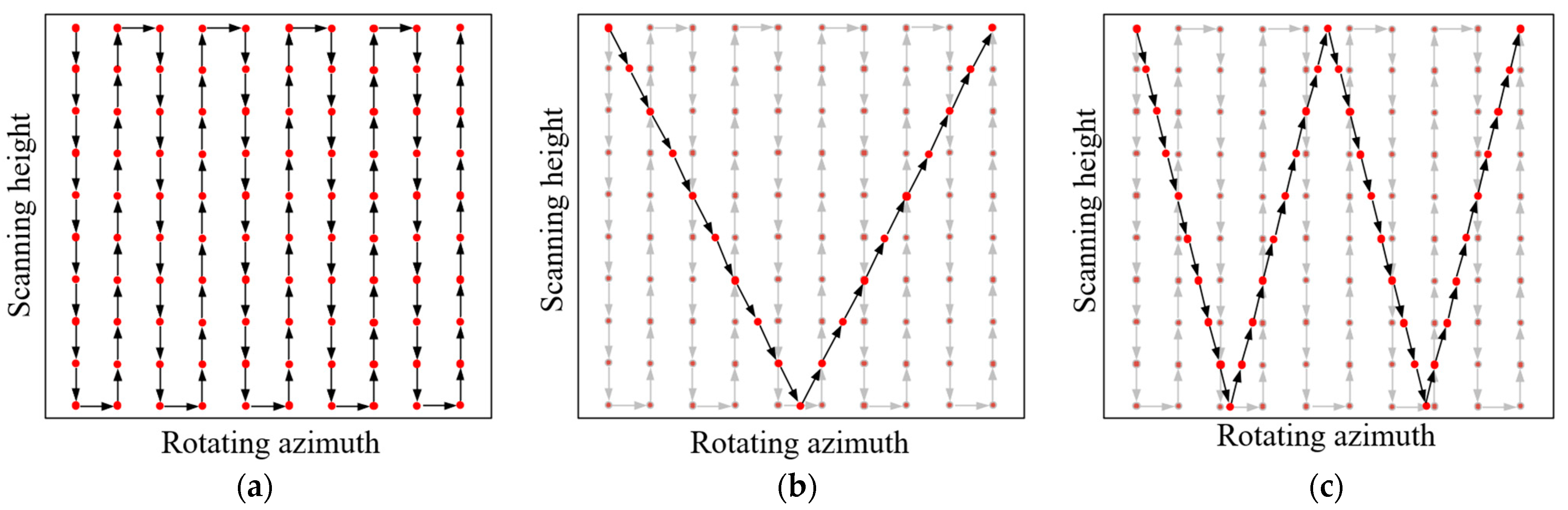
  • Development of a “V”-shaped sparse sampling trajectory and introduction of an angular–spatial joint sparse sampling model. This paper presents a “V”-shaped sparse sampling trajectory that attains generalized angular homogeneity and sufficient spatial coverage inside the angular–spatial joint domain, fulfilling the criteria for 3D imaging. A unique angular–spatial joint sparse sampling approach is developed, addressing the constraints of conventional tactics that separately consider the angular and spatial domains. By aligning the target rotation with consistent vertical stepping of the radar sensor, the model generates a non-uniform sparse sampling pattern in the joint domain. The suggested approach effectively maintains the spatial information variety by leveraging the low-rank and sparse characteristics of the target’s scattering field, while substantially decreasing the overall sampling dimension.
  • Three-dimensional image reconstruction and analysis of the minimum sampling range for the “V”-shaped sparse trajectory. This study utilizes the back-projection (BP) algorithm to assess the imaging resolution in the horizontal and sagittal planes, facilitating the optimization of parameter settings for 3D reconstruction while maintaining the image quality under diminished sampling conditions. The theoretical minimum sampling range necessary for 3D imaging is determined by the “V”-shaped sparse trajectory, which signifies the bottom limit for effective reconstruction. A comparative analysis of the imaging performance across various sampling trajectories is performed to ascertain the optimal balance among the imaging dynamic range, data volume, and acquisition time, thus offering both theoretical and practical guidance for trajectory design in real-world applications.
The subsequent sections of this paper are structured as follows. Section 2 provides the constructed “V”-shaped sparse sampling trajectory and delineates the angular–spatial joint sparse sampling model. The text outlines the system design utilizing synchronized vertical scanning and horizontal rotation, accompanied by a comprehensive examination of the 3D imaging resolution to ascertain suitable parameter settings. Section 3 delineates the experimental configuration, encompassing the system architecture and data collection methodology. Section 4 presents and analyzes the experimental results. Section 5 discusses the imaging performance and efficiency improvements achieved by the proposed sampling model, and it defines the minimum sampling range required for 3D imaging. Section 6 concludes the study.

2. Methods

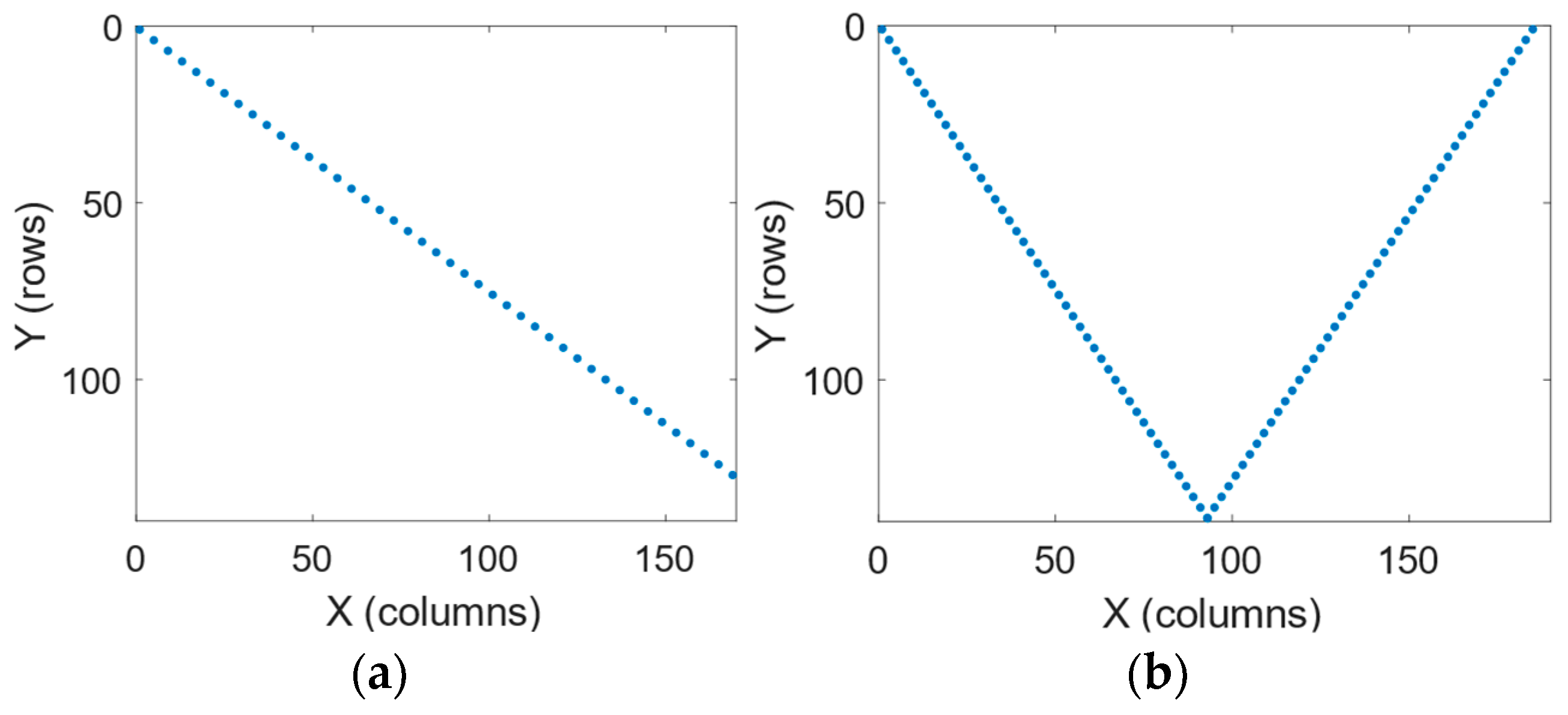
2.1. Design of the “V”-Shaped Sparse Sampling Trajectory

The aim of a three-dimensional (3D) radar imaging system is to obtain the spatial distribution of the electromagnetic scattering properties of a target in three-dimensional space. The fundamental idea involves reconstructing the volumetric scattering structure of the target by integrating echo data obtained from various viewing angles and geographical locations. Conventional cylindrical scanning systems generally utilize a full-angle sampling approach that integrates uniform angular rotation with vertical stepping. This method guarantees consistent imaging performance but frequently results in an excessive quantity of sampling points and extended acquisition duration. Consequently, there is an urgent requirement to formulate representative and diverse sampling trajectories that minimize the total number of measurements while maintaining adequate angular diversity to facilitate high-fidelity 3D reconstruction. Analysis in the angle–space joint domain reveals that any trajectory with non-redundant angular coverage can facilitate effective scattering field reconstruction, contingent upon its corresponding coverage in the wavenumber domain meeting a Nyquist-like sparsity condition [29].
The principles of 3D imaging [30] indicate that the angular span and spatial coverage of a sample trajectory directly affect the quality of the reconstructed image. The “V”-shaped trajectory exhibits a bilinear configuration in the joint angle–elevation domain, as depicted in Figure 1. The geometric design is driven by two factors: firstly, the two inclined branches allow for the collection of scattering data from two separate azimuthal directions; and secondly, the intersection point of the trajectory yields central imaging data along the elevation axis, aiding in the determination of the volumetric center of the target. Figure 1 illustrates the configuration of the “V”-shaped trajectory within the three-dimensional angular–spatial domain.
Figure 1 demonstrates that each row of the matrix signifies sampling at a consistent elevation across various azimuth angles, but each column denotes sampling at differing altitudes under a uniform azimuth angle. Each sampling point comprises a frequency-swept echo signal, creating a comprehensive three-dimensional data cube appropriate for high-resolution imaging. While the angular coverage of the synthetic aperture stays consistent, the sample intervals in both the azimuth and elevation directions vary between the traditional cylindrical scanning approach and the suggested synchronized scanning–rotation system. The “V”-shaped sample trajectories depicted in Figure 1b,c provide spatial–angular joint sampling across various viewing angles, fulfilling the minimal angular diversity necessary for precise 3D reconstruction. In contrast to the complete cylindrical trajectory, the suggested method necessitates sampling solely along two inclined pathways to obtain intersecting angular information, markedly decreasing the number of sampling sites. Furthermore, by modifying the slope and vertical increment, the sampling density and angular resolution can be dynamically optimized. Thus, the suggested method significantly decreases the total sample load while maintaining the image coverage, thereby enhancing the efficiency of radar target scattering measurements.

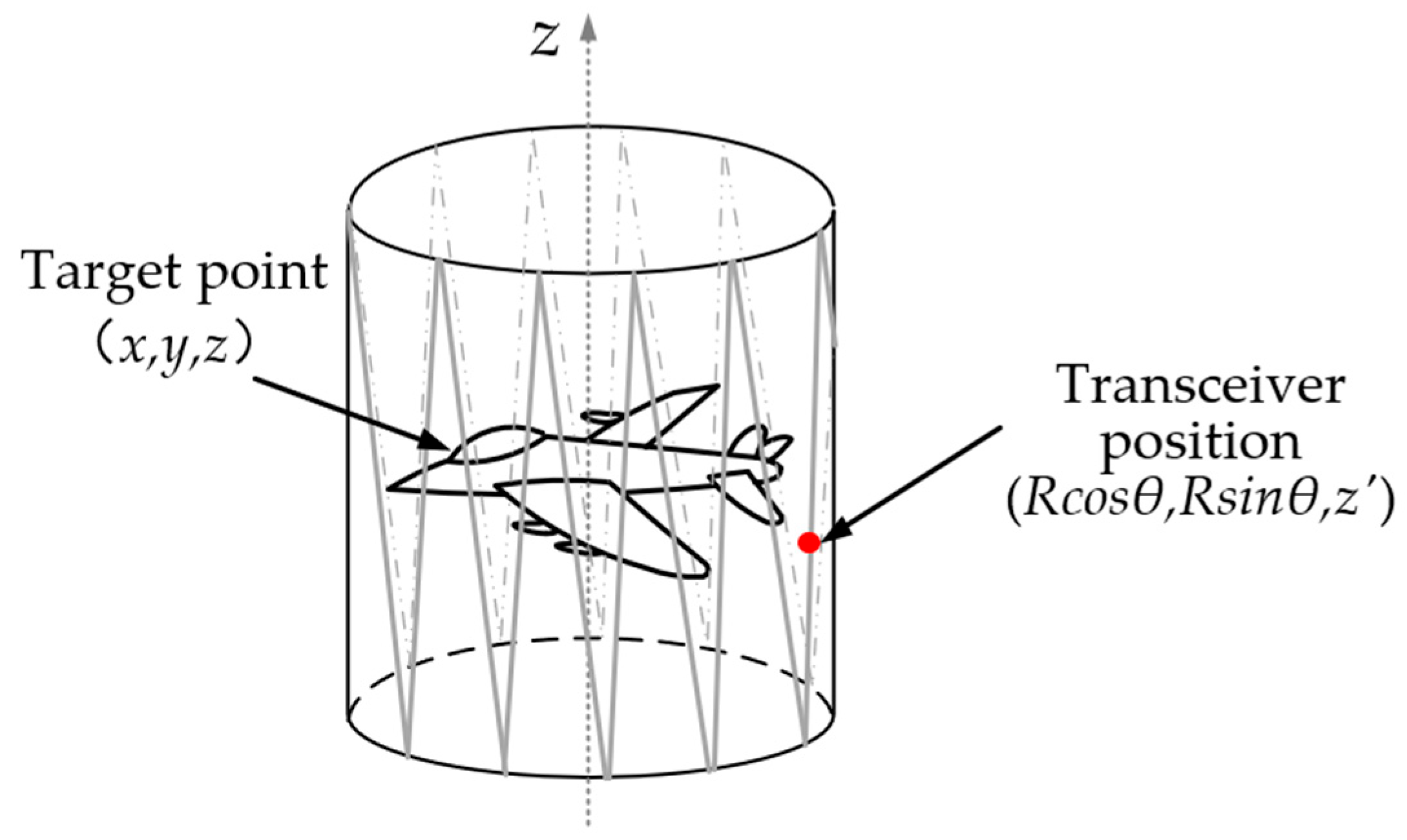
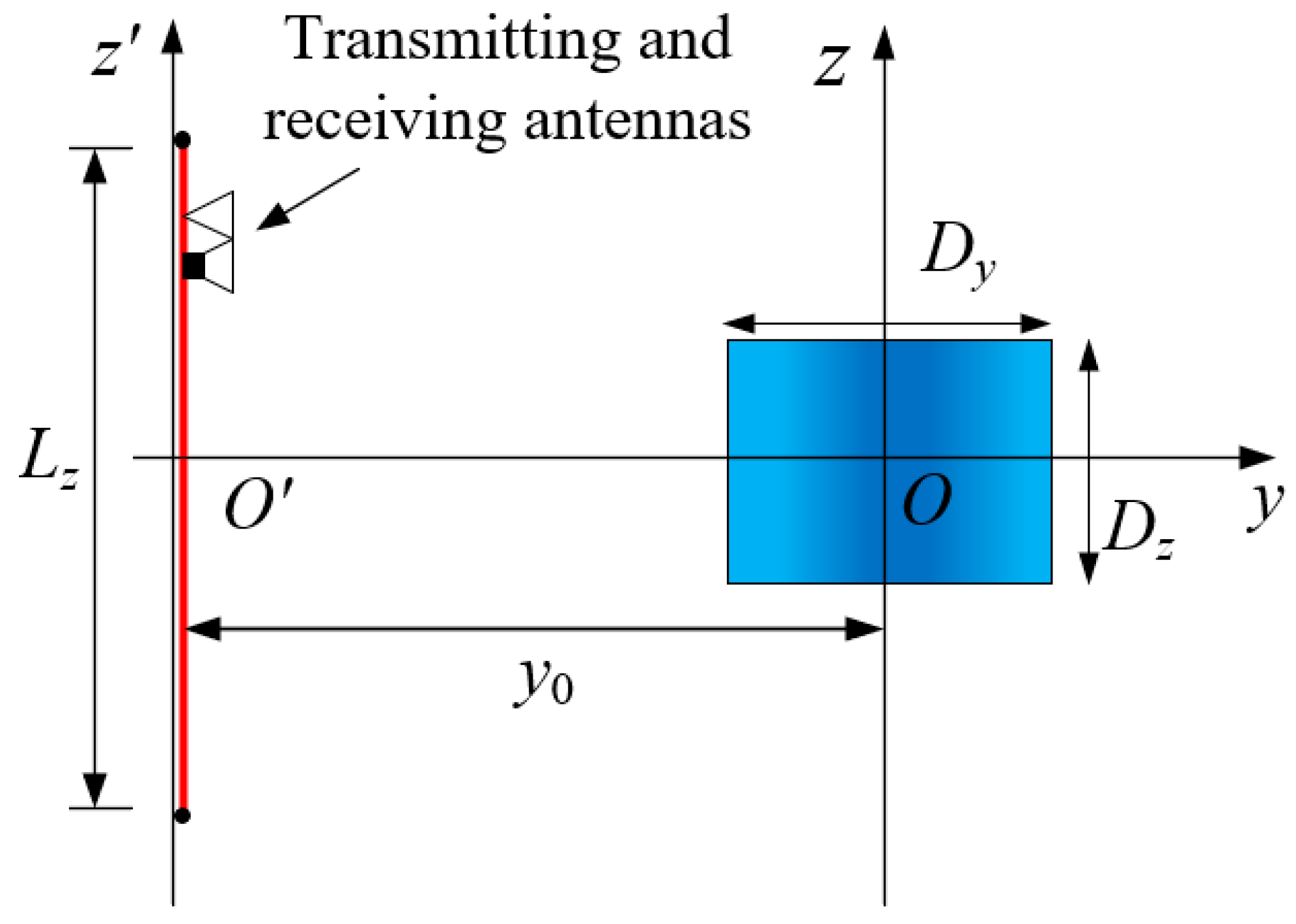
2.2. Construction of the Synchronized Scanning–Rotation Sampling Model

To facilitate synchronized sampling along the “V”-shaped trajectory, the suggested system employs the following configuration. The detector is affixed to a vertical linear guide rail, enabling linear movement along the z-axis, while the target is positioned on a motorized rotary table that rotates at a constant angular velocity. The control system synchronously activates the stepper motor and rotating table via a central controller to guarantee that each vertical sample location aligns with a designated azimuth angle. Figure 2 depicts the sampling model. The detailed procedure for synchronized scanning and rotation is depicted in the flowchart provided in Appendix A (Figure A1).
The measurement system comprises a radio frequency (RF) transceiver, a set of transmitting and receiving antennas, a vertical linear guide rail, a rotary table, and a data processing terminal. During operation, the target under test, affixed to the rotary table, experiences continuous horizontal rotation while the antenna pair concurrently conducts vertical scanning over the target. The measurement process necessitates coordinated control among the antenna array, vertical guide rail, and rotary table. The frequency-swept signal facilitates a complete vertical scan within the specified azimuthal angular range. The backscattered echoes corresponding to the synthesized motion trajectory are then acquired for processing.
Multiple coordination strategies between vertical scanning and azimuthal rotation can be utilized within the measurement system. Furthermore, since the angular separation between the transmitting and receiving antennas is under 5°, the system can be classified as quasi-monostatic.

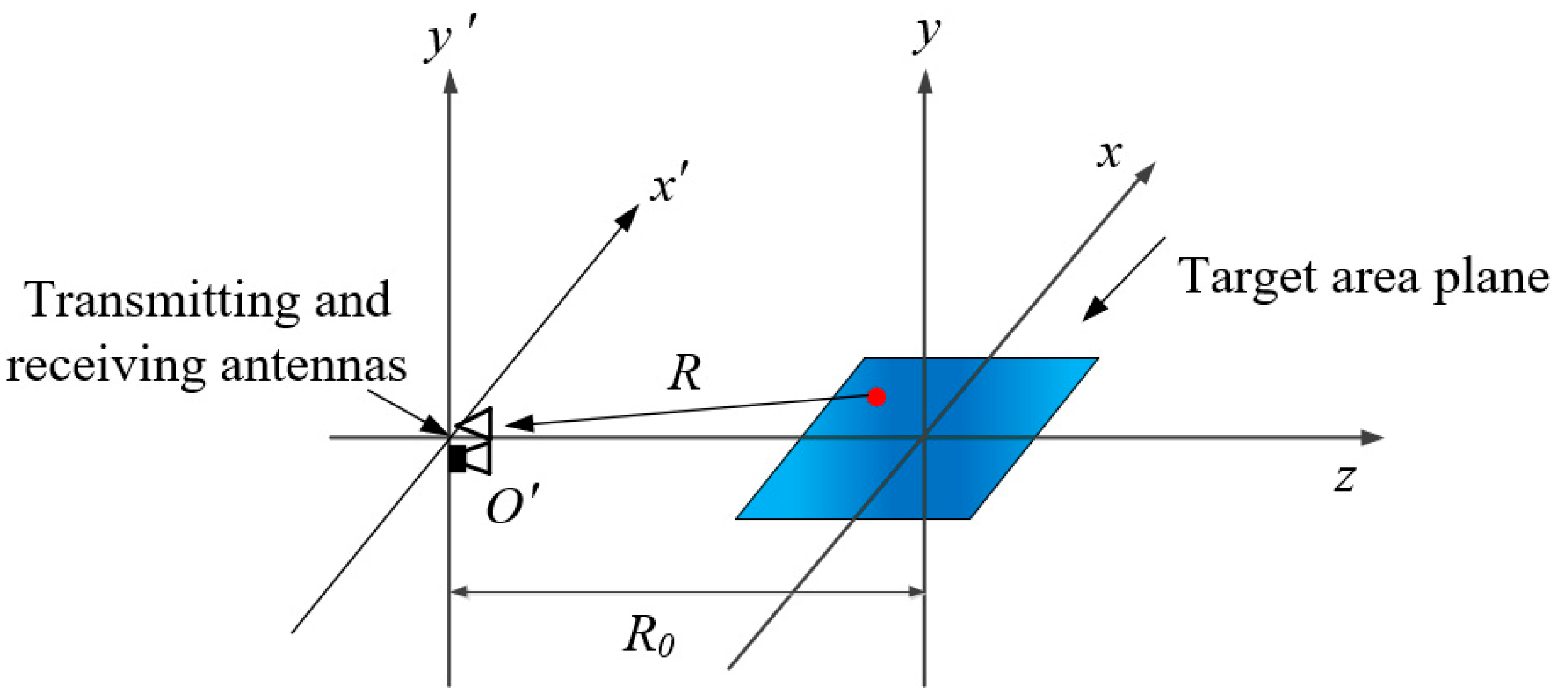
2.3. Computational Modeling for 3D Imaging

To facilitate 3D imaging using the proposed synchronized vertical scanning and azimuthal rotation measurement model, an analysis and computation of the corresponding phase compensation are required. Given that both the antenna and the radar target are in motion within this measurement setup, the direct calculation of the distance variation d between the antenna and the target is complex. An equivalent imaging model, illustrated in Figure 3, is introduced to aid in algorithmic derivation. The relative motion between the antenna and the radar target is consistent in both the physical measurement model (Figure 2) and the imaging model (Figure 3).
The imaging model illustrates that the rotation of the target on the turntable can be equivalently represented as the motion of the antenna rotating around a stationary target, as depicted in Figure 3. The antenna conducts vertical scanning concurrently throughout this process. In this equivalent configuration, the distance variation d between the antenna and the target is expressed as:
d = ( x R cos θ ) 2 + ( y R sin θ ) 2 + ( z z ) 2
The transceiver antenna performs stepped vertical scanning along the vertical rail (denoted as z ). At each scanning position, the antenna transmits stepped-frequency electromagnetic waves f . Assuming the target is located at position ( x , y , z ) , the reflected signal undergoes a phase delay 2 k d , where d represents the distance between the antenna and the target, k = 2 π f / c , and c is the speed of light. If the scattering coefficient of the target is s ( x , y , z ) , the received signal at each scanning position on the vertical axis can be expressed as:
E s ( θ , f , z ) = s ( x , y , z ) e j 2 k d d x d y d z
Based on the received electromagnetic echo signal E s ( θ , f , z ) and the theory of electromagnetic wave propagation, the target’s scattering coefficient s ( x , y , z ) can be determined accordingly.
s ( x , y , z ) = E s ( θ , f , z ) e j 2 k d d θ d f d z
In the measurement process, the echo signal E s ( θ , f , z ) is directly acquired by the receiving antenna. According to Equation (1), once the distance variation d between the antenna and the target is known, phase compensation can be applied using Equation (3) to retrieve the scattering coefficient of the radar target. This enables the proposed imaging algorithm to validate the three-dimensional reconstruction capability of the measurement model introduced in this study.

2.4. Imaging Resolution

Prior to conducting 3D imaging, it is crucial to evaluate the imaging resolution of the synchronized vertical scanning and horizontal rotation scattering measurement model, as this analysis guides the parameter settings for the imaging process. The 3D resolution analysis comprises two components: 2D imaging in the horizontal plane utilizing turntable rotation and 2D imaging in the sagittal plane employing vertical scanning. The two components represent horizontal-plane and sagittal-plane imaging, and their integration leads to 3D reconstruction. The evaluation of the range and cross-range resolutions for each 2D imaging configuration is conducted based on the principles of rotational and scanning-based imaging to determine the overall resolution characteristics of the 3D image.

2.4.1. Imaging of Target Rotation in the Horizontal Plane

In the horizontal-plane 2D image, the longitudinal and transverse resolutions are determined by the turntable-based imaging principle, as shown in Figure 4. The longitudinal resolution δ y depends on the system’s frequency bandwidth B.
δ y = c / ( 2 B )
The maximum measurable range R max is determined by the frequency domain sampling interval Δ f .
R max = c / ( 2 Δ f ) , Δ f = B / N
where N denotes the number of frequency sampling points. In practical laboratory settings, the measurement environment is typically fixed, with the target placed on a turntable at a known distance from the radar antennas. Therefore, the maximum measurable range R max can be predetermined, and the frequency domain sampling interval Δ f can be selected accordingly. The relationship is given by:
Δ f = c / ( 2 R max )
The angular dependence of the target’s scattering characteristics results in the limitation of microwave imaging to a narrow angular range. Under this condition, the approximation sin θ θ , cos θ 1 holds, and the transverse coordinate x and angular coordinate 2 θ / λ can be approximately treated as a Fourier transform pair. Based on this relationship, the transverse imaging region and resolution can be derived as follows:
x = λ 0 / ( 2 Δ θ )
For near-field measurements (point source), the transverse resolution is given by:
δ x = λ 0 / 2 Θ
where Θ denotes the angular range of the measurement. The transverse and longitudinal parameters are interconnected via resolution. Microwave imaging seeks to reconstruct the spatial distribution of a target’s reflectivity. Thus, geometric fidelity necessitates that the transverse resolution matches the longitudinal resolution. This results in the subsequent condition:
δ x = δ y
By substituting Equations (4) and (8), we obtain:
c / ( 2 B ) = λ 0 / 2 Θ
The selection of the signal bandwidth in engineering applications is primarily dictated by system performance, which is of the utmost importance. Consequently, the signal bandwidth is typically determined by the required range resolution, and the overall imaging angular aperture is subsequently computed using the aforementioned equation.
Θ = 2 B λ 0 / ( 2 c ) = B / f 0
After establishing the imaging angular range, the maximum angular step size can be computed using Equation (7), which subsequently allows for the determination of the number of angular domain samples, M. The selection of the angular step size in practical measurements must consider the positioning accuracy of the target turntable.

2.4.2. Imaging of Antenna Scanning in Sagittal Plane

Following the analysis of the resolution parameters of the horizontal-plane image generated by turntable rotation, we proceed to examine the resolution parameters of the sagittal-plane image produced by vertical antenna scanning. The resolution of two scattering points in the range direction is contingent upon the time delay between the arrival of their respective echoes at the receiving radar. Assuming one echo signal is represented by u ( t ) and the other by t d with a time delay, the resulting signal is denoted as u ( t + t d ) . The resolution capability between the two signals can then be characterized as follows:
D 2 ( t d ) = u ( t ) u ( t + t d ) 2 d t
A larger value of D 2 ( t d ) indicates better resolvability. The above expression can be expanded as:
D 2 ( t d ) = u ( t ) 2 d t + u ( t + t d ) 2 d t 2 R e u ( t ) u * ( t + t d ) d t
where * denotes complex conjugation, R e denotes taking the real part of a complex number.
u ( t ) 2 d t + u ( t + t d ) 2 d t = 2 E 0
In the equation, E 0 is a constant, so the resolution capability is determined by the autocorrelation function A ( t d ) of the signal waveform.
A ( t d ) = u ( t ) u * ( t + t d ) d t
The parameter A ( t d ) represents the distinguishability of two targets with a time delay t d ; the smaller the value of A ( t d ) , the easier it is to distinguish the targets. If the two targets completely overlap (i.e., t d = 0 ), they are evidently indistinguishable. Therefore, the resolvability at a separation of t d can be expressed by a normalized value A ( t d ) 2 / A 2 ( 0 ) . When A ( t d ) 2 / A 2 ( 0 ) = 1 , the targets are indistinguishable; if A ( t d ) 2 / A 2 ( 0 ) is slightly less than 1, the targets are difficult to distinguish; and when A ( t d ) 2 / A 2 ( 0 ) 1 , the targets are easily distinguishable. It should be noted that for a given propagation delay (i.e., distance) between two targets, the value of A ( t d ) 2 / A 2 ( 0 ) is entirely determined by the signal waveform u ( t ) . To achieve high range resolution, the autocorrelation function of the transmitted signal should be close to zero at all delays except in the vicinity of zero delay ( t d = 0 ), ideally resembling a Dirac delta function δ . The autocorrelation function and the power spectrum are related through a Fourier transform, indicating that a pronounced peak in the autocorrelation corresponds to an extensive signal bandwidth. Only wideband signals can produce a distinct output peak when processed through a matched filter or correlator. The signal bandwidth dictates the range resolution, which can be articulated as follows.
δ r 1 / B
where B denotes the bandwidth of the transmitted signal. The time delay can be converted into a range difference, allowing the range resolution to be expressed as:
δ r = c / 2 B
where c represents the propagation speed of electromagnetic waves. The azimuth resolution derivation relies on the Rayleigh resolution criterion, which indicates that two neighboring scatterers can be distinguished when their phase difference attains 360°. In this system, the azimuth resolution is attained by scanning along the vertical rail, thereby enhancing the aperture length in the azimuth direction. The resolution is derived in accordance with the Rayleigh criterion.
Assuming that two scattering points are just resolvable, the phase difference between their echoes is equal to 2 π . Accordingly, the following expression can be derived:
2 k · ( ( L z / 2 ) 2 + y 0 2 + ( L z / 2 δ z ) 2 + y 0 2 ) 2 k · ( ( L z / 2 ) 2 + y 0 2 + ( L z / 2 δ z ) 2 + y 0 2 = 2 π
The above expression can be further simplified as follows:
( L z / 2 δ z ) 2 + y 0 2 ) ( L z / 2 δ z ) 2 + y 0 2 = λ 2
Therefore, based on δ x z 0 2 + ( L x / 2 ) 2 , the equation can be rearranged as follows:
( L z / 2 δ z ) 2 + y 0 2 = y 0 2 + L z 2 / 4 L z δ z + δ z 2 y 0 2 + L z 2 / 4 L z δ z y 0 2 + L z 2 / 4 L z δ z 2 y 0 2 + L z 2 / 4
( L z / 2 + δ z ) 2 + y 0 2 = y 0 2 + L z 2 / 4 + L z δ z + δ z 2 y 0 2 + L z 2 / 4 + L z δ z y 0 2 + L z 2 / 4 + L z δ z 2 y 0 2 + L z 2 / 4
Thus, the cross-range resolution can be expressed as:
δ z = λ 0 2 L z y 0 2 + L z 2 / 4
where λ 0 is the center wavelength of the antenna, L z is the length of the scanning rail, and y 0 is the vertical distance from the rail to the target origin.
The sampling interval is a crucial parameter in imaging systems. An excessively large interval can hinder the successful reconstruction of the target image, whereas an excessively small interval prolongs the measurement time and leads to unnecessary resource consumption. It imposes increased requirements on the temporal stability of the hardware system. A schematic diagram of sagittal-plane imaging during vertical scanning is shown in Figure 5, where all the scattering points are assumed to be located within the region defined by D z / 2 , D z / 2 and D y / 2 , D y / 2 .
The sampling interval encompasses both the spatial sampling interval related to the rail and the frequency sampling interval. The Nyquist sampling rate must be determined based on the highest frequency component derived from the phase of the echo signal, as the phase of the wave varies more rapidly than its amplitude throughout the scanning process. Assuming the echo phase φ = 2 k ( z z ) 2 + ( y + y 0 ) 2 , we have:
f z = 1 2 π φ z = 2 λ ( z z ) ( z z ) 2 + ( y + y 0 ) 2
f z = 1 2 π φ k = 1 π ( z z ) 2 + ( y + y 0 ) 2
The sampling intervals in the spatial and wavenumber domains are given by:
Δ z 1 2 f z max = λ min 4 1 + ( D T y + 2 y 0 ) 2 / ( D T z + L z ) 2
Δ k 1 2 f k max = π ( D T y + 2 y 0 ) 2 + ( D T z + L z ) 2
Δ f c 2 ( D T y + 2 y 0 ) 2 + ( D T z + L z ) 2
The frequency sampling interval must not only comply with the Nyquist sampling theorem but also take into account the influencing factors of the one-dimensional (1D) range profiles. The theory of 1D range imaging posits that clean information can be acquired through techniques such as high-precision cancellation and time domain gating, provided that the target’s depth is fully represented within a single repetition period of the pulse signal. However, to effectively suppress noise, it is preferable to ensure that the target’s full depth is contained within the system’s maximum unambiguous range R = c / 2 Δ f . Let R max denote the maximum depth of the target; then, the frequency interval can be expressed as:
Δ f c 2 R max
Therefore, the determination of the frequency sampling interval should comprehensively consider both Equations (27) and (28).
The proposed three-dimensional imaging method extends two-dimensional turntable-based imaging in the horizontal plane by incorporating an additional height-scanning dimension. The analytical methods for essential parameters, including the resolution and sampling interval in 3D imaging, are analogous to those employed in 2D imaging. The resolutions in the x-direction (azimuth) and y-direction (range) are defined by Equations (8) and (17), respectively. The resolution in the z-direction (elevation) is defined as follows:
δ z = λ 2 L z y 0 2 + L z 2 / 4
The analytical approach for the sampling interval in the z-direction (elevation) mirrors that employed in the x-direction (azimuth). The subsequent expression can be derived as follows:
δ z = λ min 4 1 + ( D T y + 2 y 0 ) 2 / ( D T z + L z ) 2
where L z represents the height of the scanning frame, while D T y and D T z denote the maximum extent of the target region.
The resolution parameter settings for traditional 3D imaging align with those employed in the two previously mentioned forms of 2D imaging. The synchronized scanning and rotation sampling strategy involves the turntable rotating at a constant speed, while the transmitting and receiving antennas execute uniform vertical scanning along the rail. The resultant “V”-shaped sampling pattern, depicted in Figure 1b,c, necessitates that both the angular interval and the vertical (z-direction) spacing be reduced compared to conventional 3D imaging methods. A reduced imaging area may result in aliasing artifacts in the reconstructed image.

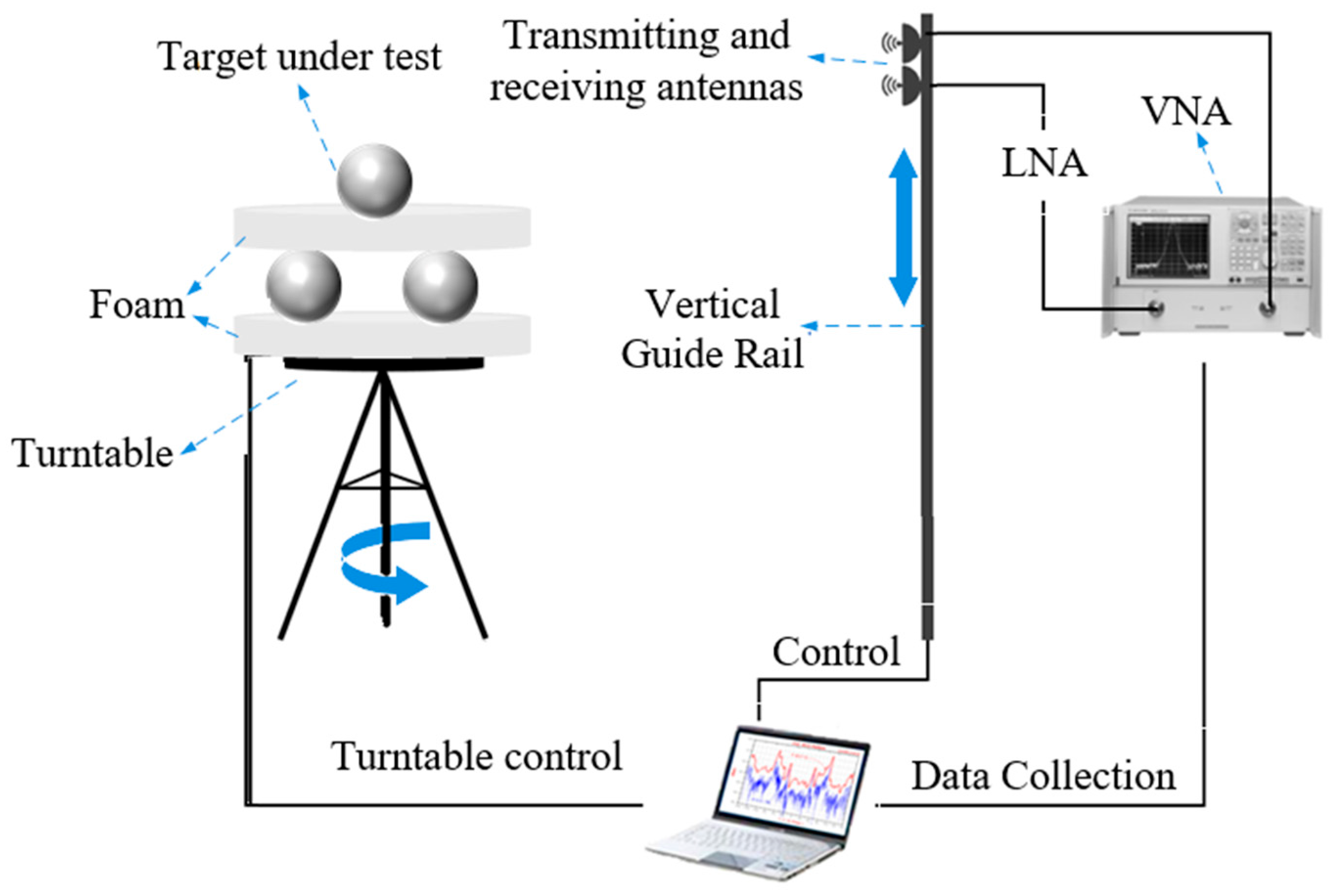
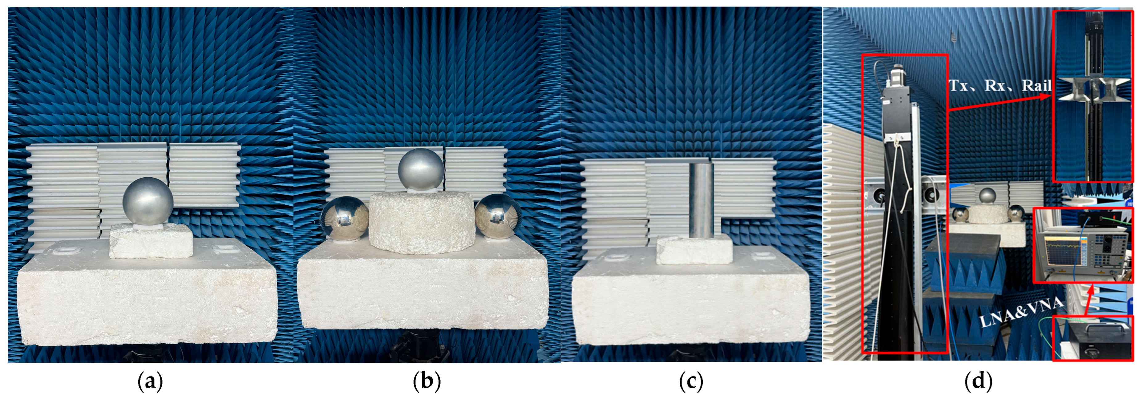
3. Experimental Setup

Figure 6 presents the schematic diagram of the testing system employed in this study. A stepped-frequency radar system consists of a two-port vector network analyzer (VNA), a low-noise amplifier (LNA), and two double-ridged horn antennas. A flat radar-absorbing material (RAM) is placed between the transmitting and receiving antennas to minimize the direct leakage between them. A foam pillar with a height of 10 cm is placed on a high-precision turntable, with the test target located at the center of both the foam pillar and the turntable. The VNA is operated through the instrumentation system to enable the transmission and reception of electromagnetic waves. The positions of the antennas and the turntable are adjusted continuously to enable the measurement of the cylindrical synthetic aperture. The scanning of the transmit–receive antenna pair and the rotation of the target commence simultaneously and continue at constant speeds to enable the formation of a “V”-shaped synthetic aperture.
Upon system setup, the initial step involves positioning the target on the foam turntable and collecting the echo data. In the second step, the target is detached from the turntable, and background echo data is collected. In the third step, the background echoes are subtracted from the target echoes, and the resultant data are utilized for 3D imaging. A laser tracker is utilized in both measurements to ensure the consistency of the turntable height.
The choice of parameters in the measurement process for 3D imaging significantly affects the quality of the resulting image. This study employs traditional cylindrical scanning-based measurement parameters, as detailed in Table 1, to maintain image integrity and achieve approximately equal lateral, longitudinal, and vertical resolutions. The spatial resolution measures 0.0375 m, with the imaging range of the target defined as 1 m × 1 m × 1 m. The angle formed by the line connecting the transmitting and receiving antennas with the target is less than 5°, indicating monostatic radar reception.
The proposed sampling schemes utilize synchronized vertical scanning and azimuthal rotation, with both motions executed at constant speeds. The vector network analyzer (VNA) manages the transmission and reception of frequency-swept signals, necessitating approximately 110 ms to collect data at each sampling position. Table 2 summarizes the sampling interval and the total number of samples for the transmitting and receiving antennas. Figure 7 illustrates various types of “V”-shaped sampling trajectories.
Figure 7a,b illustrate that the target in Sampling Schemes 1 and 2 rotates a single time within the azimuthal range. In contrast, Figure 7c illustrates that the target in Sampling Scheme 3 undergoes a clockwise rotation followed immediately by a counterclockwise rotation within the same azimuthal range. Consequently, the quantity of sampling points in Scheme 3 is double that in Scheme 2. Furthermore, all the parameter settings not specified in Table 2 are consistent with those in Table 1.
Figure 7 illustrates the blue trajectory, which denotes a complete angular rotation of the turntable in the clockwise direction, whereas the red trajectory signifies a full angular rotation in the counterclockwise direction. Additionally, Figure 7a,b exhibit an identical number of sampling points; the distinction is exclusively in the sampling trajectories, with a greater prevalence of “V”-shaped paths noted in Figure 7.

4. Experimental Results

4.1. Target Selection and Characteristics

The selected targets for the measurements are detailed in Table 3, with the corresponding images presented in Figure 8. This research utilized straightforward target models distinguished by clear scattering mechanisms. The configuration of Target 2 was designed to illustrate that, in near-field scattering measurements, various scattering sources of a target can be identified based on their spatial locations in the three-dimensional image. This confirms the applicability of the proposed method to radar target scattering diagnostics. The application of 3D imaging and scattering source extraction algorithms enables the effective acquisition of the intrinsic scattering characteristics of the target, thus enhancing the precision of target scattering measurements.
Additionally, metallic spheres and a metallic cylinder were chosen as test targets to assess the efficacy of the proposed sampling scheme for 3D imaging of various target types. A solitary metallic sphere, functioning as an isolated scattering source, was employed to validate the three-dimensional imaging technique, providing a clear scattering mechanism and intuitive imaging outcomes. A set of three metallic spheres served as a composite scattering source, whereas the cylinder functioned as a linear scattering target. The selection of these three target types, each defined by unique scattering mechanisms, aims to validate the sampling strategy and illustrate its efficacy in accurately reconstructing the three-dimensional dimensions of cylindrical objects. The chosen targets and experimental design yield significant insights regarding the impact of the sampling scheme on the 3D imaging performance.

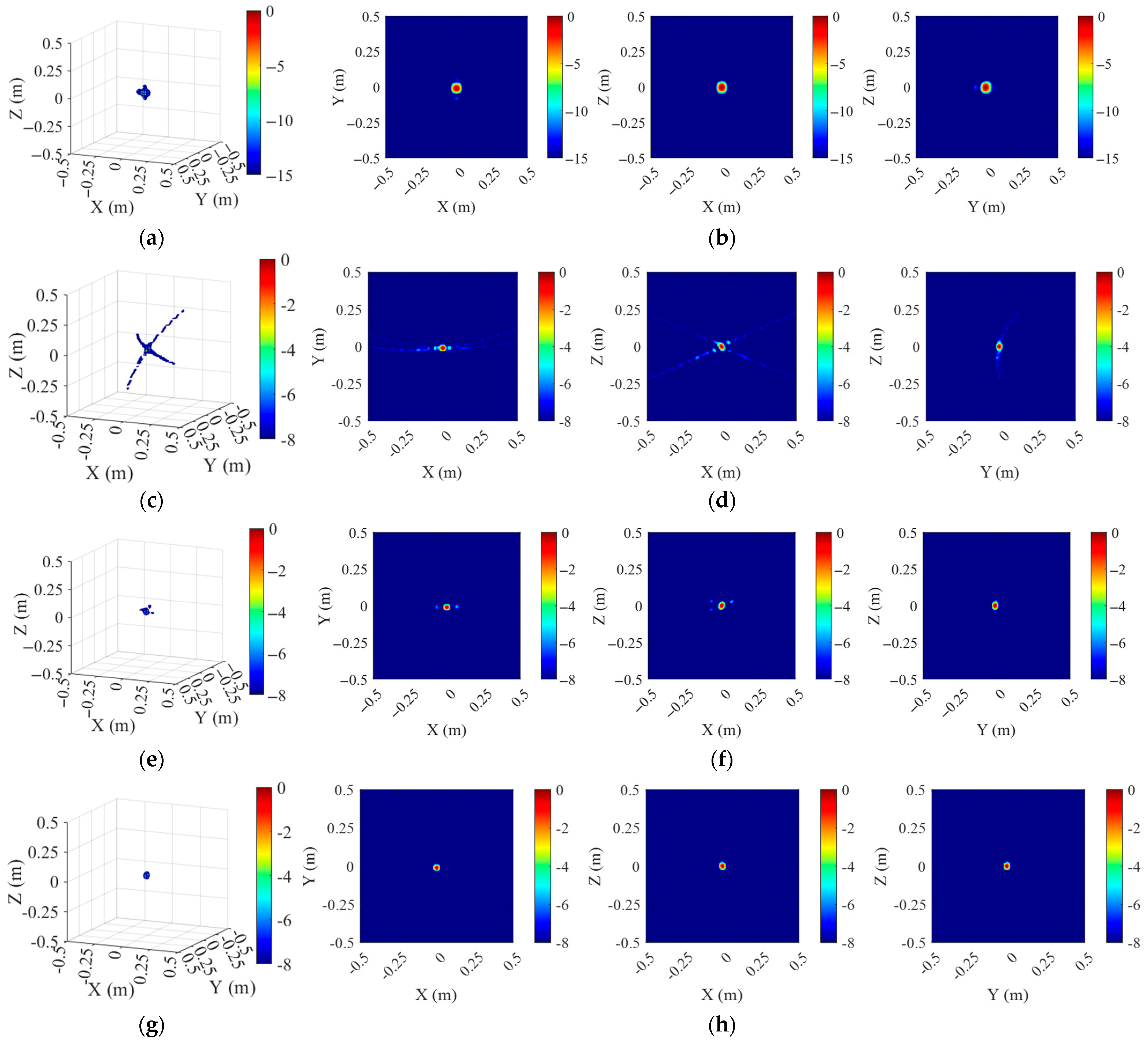
4.2. Imaging Results
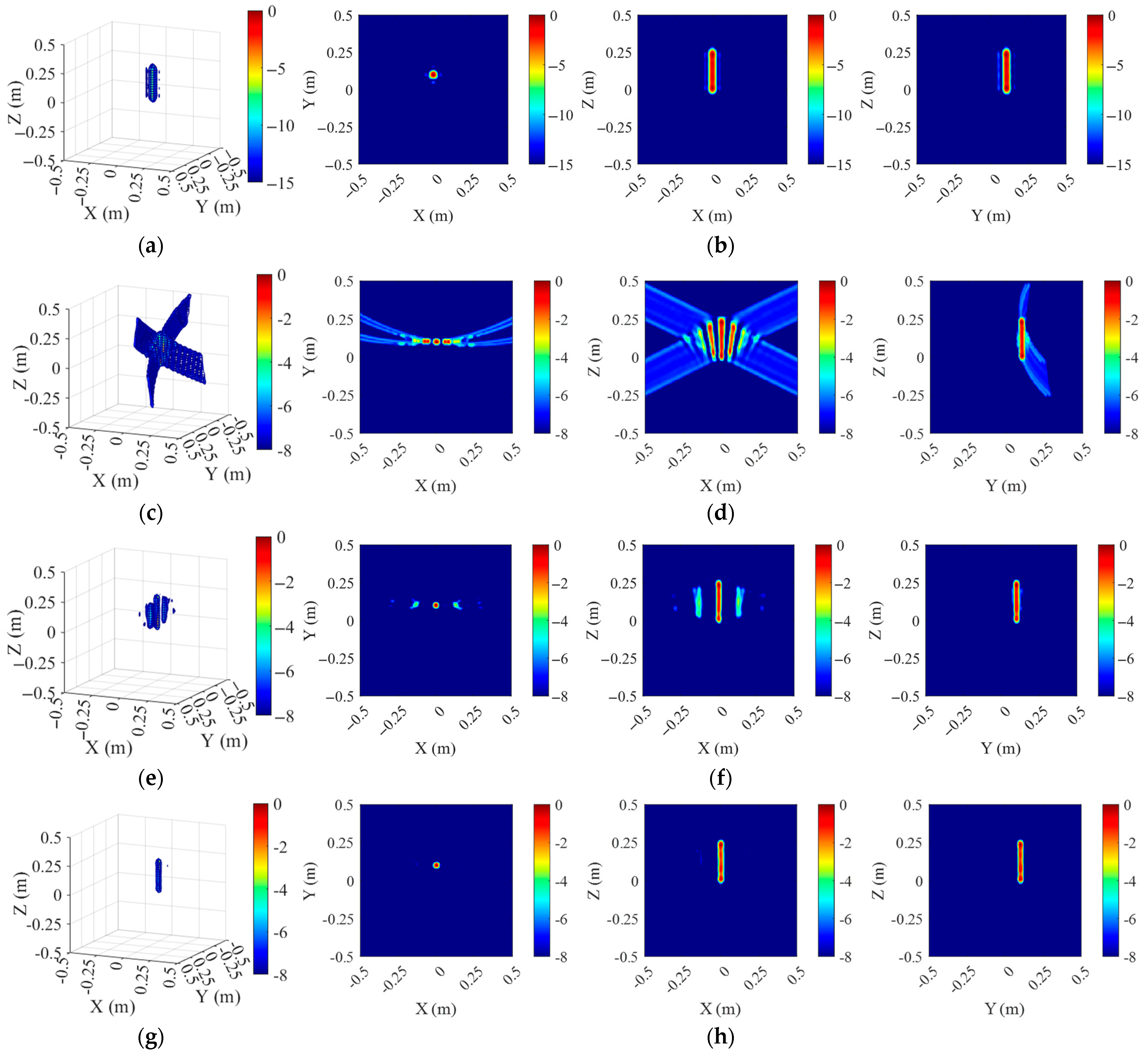
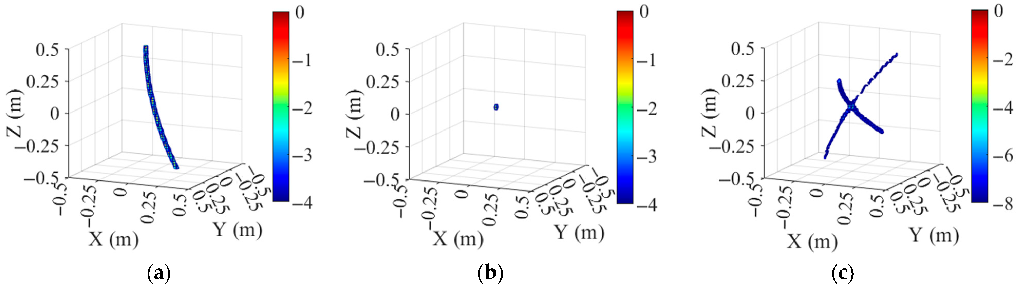
The 3D radar imaging results presented in this study are based on amplitude-normalized images, with the amplitude values quantified in decibels (dB). This normalization technique ensures that the dynamic range of the imaging data is suitable for comparison and viewing, thereby enhancing the clarity of the reconstructed images. The use of dB as a unit for amplitude enhances the ability to differentiate signal intensities, especially in the presence of noise and background interference, which is crucial for precise target detection and characterization.

4.2.1. One Sphere

Figure 9 presents the imaging results of a metallic sphere. Figure 9a presents the 3D imaging results obtained through conventional cylindrical sampling, whereas Figure 9b illustrates the associated 2D projections across three orthogonal views. Figure 9c illustrates the three-dimensional image acquired through “V”-shaped sampling utilizing synchronized scanning and rotation (Scheme 1), while Figure 9d displays its two-dimensional projections. Figure 9e,f present the three-dimensional results and two-dimensional projections derived from Scheme 2 of the synchronized scanning and rotation method. Figure 9g,h present the 3D and 2D imaging results derived from Scheme 3. The three orthogonal views of the 3D imaging results correspond to the top view, front view, and side view, respectively.
Phase compensation applied to the sampling matrices associated with various synthesized motion trajectories during measurement enables precise retrieval of the reconstructed target positions. This illustrates that the scattering measurement approach utilizing synchronized vertical scanning and azimuthal rotation of the turntable facilitates effective 3D imaging. The program was executed in MATLAB on a computer equipped with an Intel Core i7-13790F @ 2.10 GHz processor, 32 GB RAM. The program use CPU parallel acceleration. The imaging dynamic range in Figure 9c–h is uniformly set to 8 dB to facilitate a clear and intuitive comparison of the imaging performance under different sampling trajectories.
A comparison of the imaging results from sampling Schemes 1 and 2 indicates that Figure 9c,d display significant scattering clutter, leading to inferior image quality relative to Figure 9e,f, even though the number of sampling points remains constant, as detailed in Table 2. This suggests that, within the same azimuthal range of the turntable, an increase in the number of back-and-forth scans of the antenna along the vertical rail markedly enhances the imaging quality, provided the total number of samples is held constant.

4.2.2. Three Spheres

Figure 10 presents the imaging results of three metallic spheres. Figure 10a presents the 3D imaging outcome obtained through conventional cylindrical sampling, whereas Figure 10b illustrates the associated 2D projections across three orthogonal views. Figure 10c illustrates the three-dimensional image acquired through “V”-shaped sampling utilizing synchronized scanning and rotation (Scheme 1), while Figure 10d displays its two-dimensional projections. Figure 10e,f present the three-dimensional results and two-dimensional projections derived from Scheme 2 of the synchronized scanning and rotation method. Figure 10g,h present the 3D and 2D imaging results derived from Scheme 3.
The proposed sampling method is effective for 3D imaging of scattering echoes from three metallic spheres and accurately reconstructs their spatial positions. Sampling Schemes 1, 2, and 3 achieve imaging dynamic range resolutions of 6 dB, 8 dB, and 12 dB, respectively. The imaging performance aligns with that previously observed for the single metallic sphere scenario discussed earlier.

4.2.3. Cylinder

The imaging results of the metallic cylinder are presented in Figure 11. The sampling trajectories shown in Figure 11a–h are identical to those used for the single metallic sphere described above.
The imaging results for the cylinder align with those acquired for the metallic spheres, thereby reinforcing the efficacy and broad applicability of the proposed sampling scheme for three-dimensional reconstruction. The imaging results of Scheme 3, illustrated in Figure 11g,h, demonstrate a significant improvement over those of Schemes 1 and 2. Increasing the number of antenna scans along the vertical rail, as well as the total number of sampling points within the same azimuthal range of the turntable, significantly improves the quality of 3D imaging. In radar target scatterer diagnostics during maintenance, where moderate image quality is acceptable and high throughput is critical, the increase in efficiency is particularly valuable, highlighting the practical importance of the proposed sampling strategy.
Furthermore, in Figure 9, Figure 10 and Figure 11, the images in (c), (e), and (g) appear increasingly diffuse and exhibit shadowed regions compared to (a), primarily due to the use of the proposed synchronized linear scanning and rotational 3D imaging method. While this approach significantly improves the sampling efficiency and reduces the acquisition time, it inevitably compromises the imaging quality to some extent when compared to the conventional fully cylindrical sampling method. As a result, slight shadowing or reduced sharpness may appear in certain views. This issue can be mitigated by reducing the dynamic range during image rendering, which helps suppress weaker scattering outside the main lobe. Nevertheless, even under the current settings, the imaging quality remains sufficient for practical radar target recognition and engineering applications.

5. Discussion

A thorough evaluation of the proposed scheme’s imaging performance, efficiency, and minimum sampling requirements is essential.

5.1. Discussion of Imaging Result

The experimental setup utilizes a vector network analyzer (VNA) to conduct frequency sweeps ranging from 8 GHz to 12 GHz in increments of 10 MHz, resulting in 401 frequency points. At an intermediate frequency (IF) bandwidth of 5 kHz, each sweep acquisition requires approximately 110 ms. The conventional cylindrical sampling scheme involves the antenna scanning vertically at a rate of 5 mm/s for each discrete azimuth angle. The proposed synchronized scanning–rotation scheme establishes the mechanical acquisition time by utilizing the turntable’s continuous rotation across the designated azimuthal sector. Under identical frequency sweep conditions, a complete 360° rotation of the turntable requires approximately 30 min. The parameters facilitate a quantitative comparison of the measurement accuracy and acquisition efficiency between the proposed method and the conventional approach, as detailed in Table 4.
The calculation method in Table 4 allows for a comparison of the image quality and measurement efficiency across various sampling trajectories. The efficacy of ISAR imaging is often assessed using the point spread function (PSF), which characterizes the response of an imaging system to a point source, hence evaluating the resolution and sidelobe configuration of various imaging techniques [31,32]. We analyze the point spread functions of the four trajectories using MATLAB simulations, with the MATLAB software version being R2023a. The parameters utilized in the simulation are identical to those in Table 1, and the dynamic range is 15 dB.
Figure 12 illustrates the point spread functions (PSFs) associated with both the cylindrical full-sampling and the proposed sparse-sampling methods. Figure 12a presents the PSF derived from conventional cylindrical full-sampling, demonstrating superior imaging performance. Figure 12b depicts the point spread function (PSF) of Scheme 1, as shown in Figure 7, characterized by a sampling trajectory that closely resembles a single “V” shape. The resultant back-projection can be interpreted as the superposition of two cylindrical lobes, creating a “X”-shaped structure. The scattering center is notably enhanced, while off-center responses are partially canceled due to constructive and destructive interference. With an increase in the number of “V”-shaped sampling trajectories, the significance of this cancellation effect escalates. As a result, the individual cylindrical structures become indistinguishable in the PSF, as illustrated in Figure 12d, where a noticeable enhancement in imaging performance is evident.
The peak sidelobe ratio (PSLR) is defined as the ratio between the peak intensity of the most prominent sidelobe and that of the main lobe [32]. In this study, the PSLR is adopted as a quantitative metric for evaluating image quality. Table 5 summarizes the approximate PSLR values (with the estimation errors within 1 dB) corresponding to the sampling trajectories investigated in this work, providing a basis for quantitatively assessing the imaging performance of each scheme.
Table 5 demonstrates that the proposed sparse sampling Scheme 3 surpasses Schemes 1 and 2 regarding the imaging quality. The proposed sparse sampling strategies demonstrate a marked reduction in the acquisition time compared to the conventional cylindrical full-sampling approach, albeit with a minor decline in the PSLR. Table 6 presents a comprehensive comparison of the measurement efficiency.
The synchronized scanning–rotation sampling Schemes 2 and 3 achieve 3D imaging with dynamic ranges of 7 dB and 12 dB, respectively, deemed appropriate for practical engineering applications. Table 6 illustrates that Scheme 3 decreases the number of sampling points by 75% and enhances the measurement efficiency by over 94%. In practical scattering measurements, the system parameters may be modified to enhance the balance between imaging quality and acquisition efficiency.
While the proposed sparse sampling strategy significantly improves the acquisition efficiency, it inherently leads to a reduction in the peak sidelobe ratio (PSLR), which in turn limits the effective dynamic range of the reconstructed image. A lower dynamic range may impact several critical aspects of practical radar imaging. First, a reduced dynamic range can affect the calibration accuracy, especially in systems where strong targets dominate and overshadow subtle structural or amplitude variations. This may lead to underestimation of weaker scatterers or misinterpretation of background reflections during system calibration. Second, the sensitivity to weak targets is inherently diminished. When the dynamic range is compressed, the weaker scattering centers may fall below the sidelobe floor or noise threshold, resulting in reduced visibility or complete loss of low RCS (radar cross-section) features. Third, in low SNR scenarios, dynamic range limitations can exacerbate the difficulty of distinguishing signal from noise. The presence of stronger sidelobes may mask weak target responses, leading to degraded detection capability and increased false alarms. These effects underscore a trade-off in the current method: while the proposed sparse sampling scheme delivers substantial gains in measurement speed and engineering simplicity, it also introduces limitations in imaging fidelity, particularly under challenging electromagnetic conditions. To address these issues, future work may integrate adaptive reconstruction algorithms and dynamic range-aware processing strategies. Additionally, incorporating AI-driven denoising or super-resolution techniques may further enhance the reconstruction quality without compromising efficiency. These directions will help mitigate the limitations of a reduced PSLR while preserving the practicality and cost-effectiveness of the proposed method.
This study concentrates on principle-level validation in controlled laboratory conditions, employing standard measurement equipment and optimal mechanical motion settings to illustrate the efficacy of the proposed sparse sampling strategy. The parameter settings employed in the imaging resolution analysis are also relevant when applied to the measurement of large-scale or complex targets. We acknowledge that the adaptability and scalability of the proposed method require further evaluation for practical engineering deployment. In practical field applications, factors such as timing jitter and mechanical vibration may occur, necessitating precise motion tracking and positioning during the scanning process. Furthermore, integration with diverse radar systems, encompassing multi-band or non-standard scanning architectures, must be taken into account. Future research will concentrate on integrating fault-tolerant synchronization techniques, motion compensation algorithms, and scalable sampling frameworks to facilitate the robust implementation of the proposed method across various complex measurement platforms.
Furthermore, the implementation of the proposed sparse sampling scheme in practical engineering contexts may encounter challenges, including noise robustness, scatterer localization errors, and imaging artifacts. Consequently, systematic engineering evaluations are necessary to evaluate and resolve these system-level issues. Future research will concentrate on the development of adaptive calibration techniques, noise-aware reconstruction algorithms, and artifact suppression strategies to improve the robustness and reliability of the proposed method across diverse sampling conditions.

5.2. The Minimum Sampling Range

This section further examines the minimum sampling extent necessary to ensure reliable 3D imaging using the validated synchronized scanning–rotation sampling scheme, which has demonstrated the capability to achieve acceptable engineering-level image quality and enhanced measurement efficiency. Three-dimensional microwave imaging necessitates range information obtained through stepped-frequency excitation and two distinct spatial sampling dimensions to reconstruct the cross-range distribution of the scattering centers. The synchronized scanning–rotation sampling scheme necessitates the generation of at least one “V”-shaped trajectory that integrates continuous azimuthal rotation with vertical rail scanning. This motion synthesizes a two-dimensional aperture surface in the ( θ , z ) domain and supplies the complete phase history needed for accurate back-projection or Fourier-based 3D reconstruction.
Limiting the sampling path to a single linear trajectory results in the acquisition of only one spatial degree of freedom, leading to a collapse of spatial frequency support and significant ambiguities in the reconstructed image. Figure 13 illustrates the linear and “V”-shaped trajectories, while Table 7 lists the measurement parameters. The corresponding measured results for a single sphere are presented in Figure 14.
Figure 14a demonstrates improper imaging of the sphere, resulting in a singular line representation. Figure 14b illustrates the point at which the target becomes distinguishable, while Figure 14c, with an increased dynamic range, reveals an “X” shape in the image. The intersection of the two lines accurately represents the position of the target. The results indicate that a single “V”-shaped trajectory represents the minimum sampling aperture necessary for the proposed scheme to facilitate 3D imaging. The “V”-shaped path provides adequate angular diversity for localizing scatterers across all three spatial dimensions, while a single slanted trajectory is insufficient for this task.

6. Conclusions

This study examines efficient sampling strategies for 3D radar imaging, beginning with the design of a “V”-shaped sampling trajectory that is straightforward to implement and replicate on a practical testing platform. A spatial sampling method that integrates synchronized vertical scanning and horizontal rotation is proposed based on this trajectory. The proposed approach constructs a joint angle–space modeling framework that effectively reduces the overall number of sampling points while significantly enhancing the imaging efficiency, all while maintaining a reasonable dynamic range. The experimental results indicate that this method surpasses traditional cylindrical sampling in reconstructing target scattering characteristics, achieving a 75% reduction in sampling quantity and a 94% reduction in sampling time.
This study advances high-resolution 3D radar imaging technologies through two key areas: coordinated motion modeling and trajectory optimization. This study assesses the feasibility and robustness of sparse sampling in practical imaging applications. The proposed strategy effectively addresses the engineering challenge of balancing imaging performance, efficiency, and precision, indicating significant potential for engineering applications. It is worth noting that the current validation is limited to canonical targets under ideal, clutter-free conditions. A comprehensive quantitative evaluation involving large-scale, distributed, or realistic targets—particularly in complex outdoor environments affected by clutter, multipath propagation, and other environmental factors—remains essential. Such field-level experiments constitute the next phase of the engineering validation and are critical for demonstrating the generalizability and practical applicability of the proposed methodology in real-world scenarios.
Future research will focus on investigating the sparsity of measurement targets and enhancing the resolution while maintaining the existing sampling scheme and duration. Future research may concentrate on systematic error modeling, adaptive trajectory design, and joint optimization with AI-based reconstruction algorithms to enhance the practical implementation of low-cost, high-efficiency, and high-precision radar imaging systems.

Author Contributions

Conceptualization, C.L. and J.Z.; data curation, X.W., Y.Z. and J.L.; formal analysis, C.L. and Z.Y.; investigation, X.W. and Z.Y.; methodology, C.L. and J.Z.; software, C.L.; supervision, J.M. and J.Z.; validation, C.L., Y.Z. and J.L.; writing—original draft, C.L.; writing—review and editing, J.Z., Z.Y. and X.W. All authors have read and agreed to the published version of the manuscript.

Funding

This research received no external funding.

Data Availability Statement

The data presented in this study are available on request from the corresponding author.

Acknowledgments

Thanks to the editors and reviewers for their careful review, constructive suggestion and reminders, which helped improve the quality of the paper.

Conflicts of Interest

The authors declare no conflicts of interest.

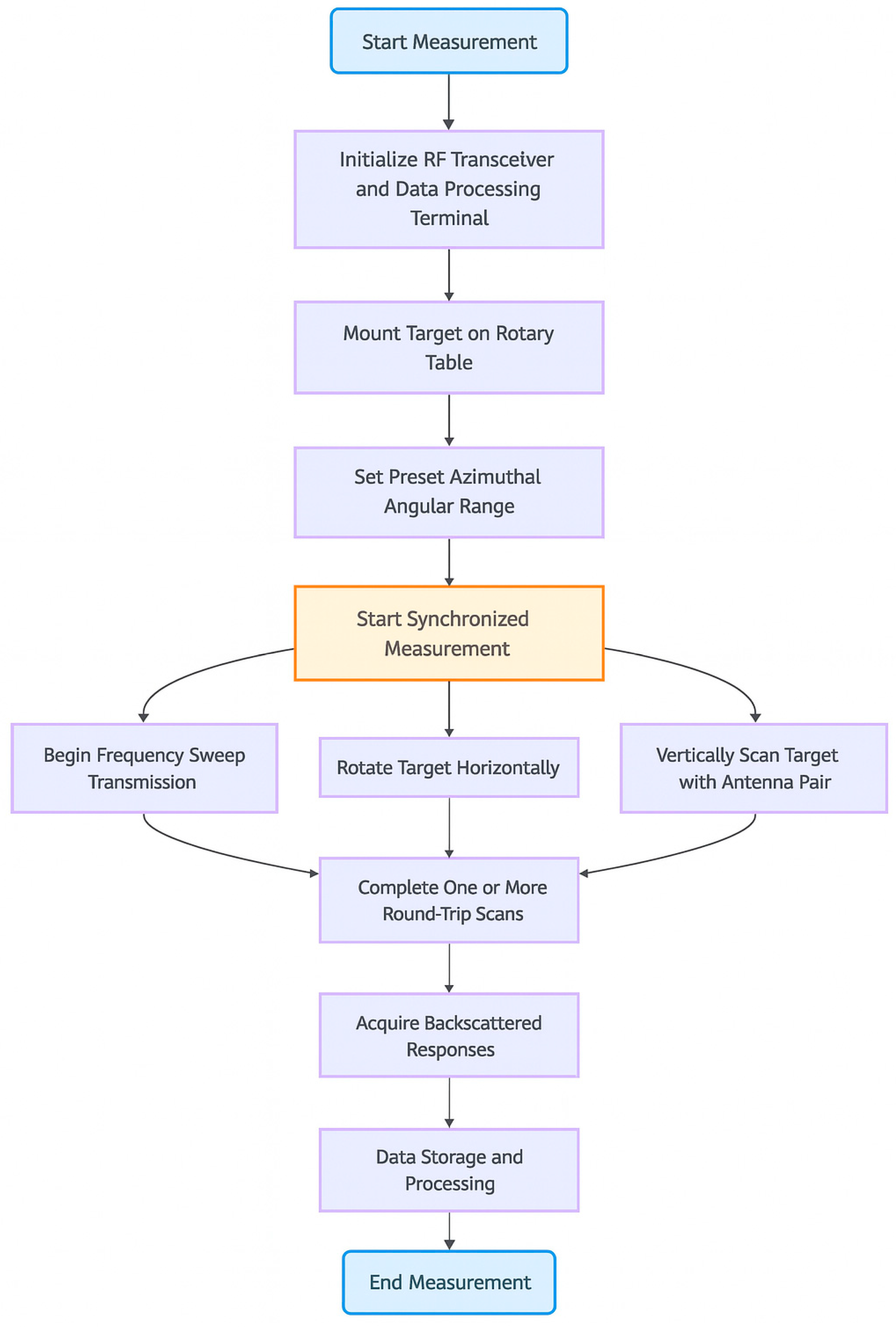
Appendix A. Measurement Process Flowchart

This flowchart depicts the synchronized measurement strategy employed in this study. In the measurement process, the transmitting antenna conducts a frequency sweep, the rotary table rotates the target horizontally, and the antenna pair simultaneously perform vertical scanning. The coordinated motions facilitate efficient acquisition of the backscattered responses across the specified angular domain.
Figure A1. Flowchart of the synchronized measurement process combining frequency sweep transmission, azimuthal rotation of the target, and vertical scanning by the antenna pair.
Remotesensing 17 02636 g0a1

References

  1. Meng, X.; Xue, M.; Wang, Z. Microwave 3-D imaging echo simulation for discrete targets. Electron. Meas. Technol. 2007, 8, 37–40. [Google Scholar]
  2. Mensa, D.L. High Resolution Radar Cross-Section Imaging; Artech House: Boston, MA, USA, 1991; Volume 1, p. 280. [Google Scholar]
  3. Tan, W.; Hong, W.; Wang, Y.; Wu, Y. A novel spherical-wave three-dimensional imaging algorithm for microwave cylindrical scanning geometries. Prog. Electromagn. Res. 2011, 111, 43–70. [Google Scholar] [CrossRef]
  4. Falconi, M.T.; Comite, D.; Galli, A.; Pastina, D.; Lombardo, P.; Marzano, F.S. Forward Scatter Radar for Air Surveillance: Characterizing the Target-Receiver Transition from Far-Field to Near-Field Regions. Remote Sens. 2017, 9, 50. [Google Scholar] [CrossRef]
  5. Hu, C.; Li, N.; Chen, W.; Zhang, L. High-precision RCS measurement of aircraft’s weak scattering source. Chin. J. Aeronaut. 2016, 29, 772–778. [Google Scholar] [CrossRef]
  6. Jain, A.; Patel, I. Dynamic imaging and RCS measurements of aircraft. IEEE Trans. Aerosp. Electron. Syst. 1995, 31, 211–226. [Google Scholar] [CrossRef]
  7. Yang, Z.; Zhao, J.; Si, W.; Lou, C.; Zhao, X.; Miao, J. A Target Near-Field Scattering Measurement Technique Utilizing 3D Near-Field Imaging via Cylindrical Scanning. Remote Sens. 2025, 17, 1575. [Google Scholar] [CrossRef]
  8. Ding, Z.; Zhang, T.; Li, Y.; Li, G.; Dong, X.; Zeng, T.; Ke, M. A ship ISAR imaging algorithm based on generalized radon-Fourier transform with low SNR. IEEE Trans. Geosci. Remote Sens. 2019, 57, 6385–6396. [Google Scholar] [CrossRef]
  9. Liu, F.; Huang, D.; Guo, X.; Feng, C. Translational motion compensation for maneuvering target echoes with sparse aperture based on dimension compressed optimization. IEEE Trans. Geosci. Remote Sens. 2022, 60, 3169275. [Google Scholar] [CrossRef]
  10. Ren, L.; Mills, J.K.; Sun, D. Trajectory tracking control for a 3-DOF planar parallel manipulator using the convex synchronized control method. IEEE Trans. Control Syst. Technol. 2008, 16, 613–623. [Google Scholar] [CrossRef]
  11. Xu, G.; Zhang, B.; Yu, H.; Chen, J.; Xing, M.; Hong, W. Sparse synthetic aperture radar imaging from compressed sensing and machine learning: Theories, applications, and trends. IEEE Geosci. Remote Sens. Mag. 2022, 10, 32–69. [Google Scholar] [CrossRef]
  12. Wang, Y.; Zhang, X.; Zhan, X.; Zhang, T.; Zhou, L.; Shi, J.; Wei, S. An RCS measurement method using sparse imaging based 3-D SAR complex image. IEEE Antennas Wirel. Propag. Lett. 2021, 21, 24–28. [Google Scholar] [CrossRef]
  13. He, Y.; Zhang, D.; Chen, Y. 3d radio imaging under low-rank constraint. IEEE Trans. Circuits Syst. Video Technol. 2023, 33, 3833–3847. [Google Scholar] [CrossRef]
  14. Zhang, X.; Lomas, A.; Zhou, M.; Zheng, Y.; Curtis, A. 3-D Bayesian variational full waveform inversion. Geophys. J. Int. 2023, 234, 546–561. [Google Scholar] [CrossRef]
  15. Park, J.; Raj, R.G.; Martorella, M.; Giusti, E. Multilook polarimetric 3-D interferometric ISAR imaging. IEEE Trans. Aerosp. Electron. Syst. 2022, 58, 5937–5943. [Google Scholar] [CrossRef]
  16. Dou, Y.Y.; Wu, Y.M.; Jin, H.Q.; Jin, Y.Q.; Hu, J.; Cheng, J. The efficient norm regularization method applying on the ISAR image with sparse data. IEEE Trans. Geosci. Remote Sens. 2022, 60, 3218581. [Google Scholar] [CrossRef]
  17. Huang, P.; Xia, X.G.; Zhan, M.; Liu, X.; Liao, G.; Jiang, X. ISAR imaging of a maneuvering target based on parameter estimation of multicomponent cubic phase signals. IEEE Trans. Geosci. Remote Sens. 2021, 60, 3091645. [Google Scholar] [CrossRef]
  18. Shin, H.S.; Lim, J.T. Omega-K algorithm for spaceborne spotlight SAR imaging. IEEE Geosci. Remote Sens. Lett. 2011, 9, 343–347. [Google Scholar] [CrossRef]
  19. Yan, W.; Xu, J.D.; Li, N.J.; Tan, W. A novel fast near-field electromagnetic imaging method for full rotation problem. Prog. Electromagn. Res. 2011, 120, 387–401. [Google Scholar] [CrossRef]
  20. Wang, W.; Zhang, H.; Zhang, Z.; Liu, L.; Shao, L. Sparse graph based self-supervised hashing for scalable image retrieval. Inf. Sci. 2021, 547, 622–640. [Google Scholar] [CrossRef]
  21. Li, D.; Zhan, M.; Liu, H.; Liao, Y.; Liao, G. A robust translational motion compensation method for ISAR imaging based on keystone transform and fractional Fourier transform under low SNR environment. IEEE Trans. Aerosp. Electron. Syst. 2017, 53, 2140–2156. [Google Scholar] [CrossRef]
  22. Wang, X. DBN-FTLSTM: An Optimized Deep Learning Framework for Speech and Image Recognition. Informatica 2025, 49, 8169. [Google Scholar] [CrossRef]
  23. Zhang, Q.; Bai, J.; Chang, X. Pioneering Testing and Assessment Framework For AI-Powered SAR ATR Systems. In Proceedings of the 2024 IEEE 7th International Conference on Big Data and Artificial Intelligence (BDAI), Beijing, China, 5–7 July 2024; pp. 230–234. [Google Scholar]
  24. Gu, T.; Guo, Y.; Zhao, C.; Zhang, J.; Zhang, T.; Liao, G. Thorough Understanding and 3D Super-Resolution Imaging for Forward-Looking Missile-Borne SAR via a Maneuvering Trajectory. Remote Sens. 2024, 16, 3378. [Google Scholar] [CrossRef]
  25. Xing, S.; Song, S.; Quan, S.; Sun, D.; Wang, J.; Li, Y. Near-field 3D sparse SAR direct imaging with irregular samples. Remote Sens. 2022, 14, 6321. [Google Scholar] [CrossRef]
  26. Neitz, O.; Mauermayer, R.A.; Eibert, T.F. 3-D monostatic RCS determination from multistatic near-field measurements by plane-wave field synthesis. IEEE Trans. Antennas Propag. 2019, 67, 3387–3396. [Google Scholar] [CrossRef]
  27. Wang, J.; Liu, X. Improved global range alignment for ISAR. IEEE Trans. Aerosp. Electron. Syst. 2007, 43, 1070–1075. [Google Scholar] [CrossRef]
  28. Lv, M.; Chen, W.; Ma, J.; Yang, J.; Ma, X.; Cheng, Q. Joint random stepped frequency ISAR imaging and autofocusing based on 2D alternating direction method of multipliers. Signal Process. 2022, 201, 108684. [Google Scholar] [CrossRef]
  29. Righero, M.; Giordanengo, G.; Ciorba, L.; Vecchi, G. Fast antenna characterization with numerical expansion functions built with partial knowledge of the antenna and accelerated asymptotic methods. IEEE Trans. Antennas Propag. 2022, 71, 970–983. [Google Scholar] [CrossRef]
  30. Udupa, J.K. 3D imaging: Principles and approaches. In 3D Imaging in Medicine, 2nd ed; Routledge: New York, NY, USA, 2023; pp. 1–73. [Google Scholar]
  31. Knaell, K.; Cardillo, G. Radar tomography for the generation of three-dimensional images. IEE Proc. Radar Sonar Navig. 1995, 142, 54–60. [Google Scholar] [CrossRef]
  32. Tan, W.; Hong, W.; Wang, Y.; Lin, Y.; Wu, Y. Synthetic aperture radar tomography sampling criteria and three-dimensional range migration algorithm with elevation digital spotlighting. Sci. China Ser. F Inf. Sci. 2009, 52, 100–114. [Google Scholar] [CrossRef]
Figure 1. Illustration of different composite sampling trajectories: (a) traditional cylindrical sampling trajectory; (b) “V”-shaped sampling trajectory; and (c) “VV”-shaped sampling trajectory.
Remotesensing 17 02636 g001
Figure 2. Schematic of the synchronized vertical scanning and azimuthal rotation system for scatterer diagnostics.
Remotesensing 17 02636 g002
Figure 3. Illustration of the imaging model based on synchronized scanning and rotational motion.
Remotesensing 17 02636 g003
Figure 4. Illustration of horizontal-plane 2D imaging based on turntable rotation.
Remotesensing 17 02636 g004
Figure 5. Illustration of sagittal-plane 2D imaging based on vertical scanning.
Remotesensing 17 02636 g005
Figure 6. The diagram of the testing system.
Remotesensing 17 02636 g006
Figure 7. Illustration of three “V”-shaped sampling schemes: (a) sampling trajectory matrix of Scheme 1; (b) sampling trajectory matrix of Scheme 2; and (c) sampling trajectory matrix of Scheme 3.
Remotesensing 17 02636 g007
Figure 8. The chosen targets in the study showing: (a) Target 1; (b) Target 2; (c) Target 3; and (d) experimental measurement scenarios.
Remotesensing 17 02636 g008
Figure 9. Imaging result of a sphere. (a) The 3D image and (b) the orthogonal views of the conventional cylindrical sampling; (c) the 3D image and (d) the orthogonal views of the sampling Scheme 1; (e) the 3D image and (f) the orthogonal views of the sampling Scheme 2; and (g) the 3D image and (h) the orthogonal views of the sampling Scheme 3.
Remotesensing 17 02636 g009
Figure 10. Imaging result of three spheres. (a) The 3D image and (b) the orthogonal views of the conventional cylindrical sampling; (c) the 3D image and (d) the orthogonal views of the sampling Scheme 1; (e) the 3D image and (f) the orthogonal views of the sampling Scheme 2; and (g) the 3D image and (h) the orthogonal views of the sampling Scheme 3.
Remotesensing 17 02636 g010
Figure 11. Imaging result of a cylinder. (a) The 3D image and (b) the orthogonal views of the conventional cylindrical sampling; (c) the 3D image and (d) the orthogonal views of the sampling Scheme 1; (e) the 3D image and (f) the orthogonal views of the sampling Scheme 2; and (g) the 3D image and (h) the orthogonal views of the sampling Scheme 3.
Remotesensing 17 02636 g011
Figure 12. PSFs of different sampling trajectories. (a) The traditional cylindrical sampling, (b) Scheme 1, (c) Scheme 2 and (d) Scheme 3.
Remotesensing 17 02636 g012
Figure 13. The sampling trajectory of the proposed method. (a) The linear and (b) “V”-shaped trajectories.
Remotesensing 17 02636 g013
Figure 14. Three-dimensional imaging result of a sphere. (a) “\”-shaped sampling with a 4 dB dynamic range; (b) “V”-shaped sampling with a 4 dB dynamic range; and (c) “V”-shaped sampling with an 8 dB dynamic range.
Remotesensing 17 02636 g014
Table 1. Test parameters for traditional cylindrical scanning-based 3D imaging.
SymbolParameterDescription
P VVPolarization Mode of the Antenna
R 2 mDistance from the Antenna to the Target Center
B 4 GHzSweep Bandwidth
f c 10 GHzCenter Frequency
Θ 23.52°Angular Sweep Range
L z 0.828 mRail Length
Θ N 1Number of Round-Trip Samplings on the Turntable
L N 29Number of Round-Trip Samplings Along the Rail
Δ f 10 MHzFrequency Interval
Δ θ 0.84°Angular Interval
Δ z 0.018 mRail Scanning Interval
N 401Number of Frequency Sampling Points
M 29Number of Angular Sampling Points
K 47Number of Rail Sampling Points
T 1363Total Number of Samples M × K
Table 2. Test parameters for 3D imaging using the proposed sampling schemes.
SymbolScheme 1 1Scheme 2 1Scheme 3 1
Δ θ 0.14°0.14°0.14°
Δ z 0.012 m0.018 m0.018 m
Θ N 112
L N 348
T 169169338
1 The sampling schemes are illustrated in Figure 7.
Table 3. Target information.
TargetDimensionsPose
One SphereRadius: 5.64 cmVertical
Three SpheresRadius: 5.64 cm
Radius: 5.64 cm
Radius: 5.64 cm
Vertical
CylinderRadius: 5.2 cm
Height: 30.1 cm
Horizontal
Table 4. The parameters for the sampling efficiency calculation.
SymbolParameterDescription
T 1 1363Total number of traditional cylindrical samples
T 2 169 or 338Total number of “V”-shaped sampling
T D 110   ms × T The data acquisition time with VNA
T M 1 ( L z ÷ 5   mm / s ) × M Mechanical motion time of traditional cylindrical sampling
T M 2 ( 30   min ÷ 360 ) × Θ N Mechanical motion time of “V”-shaped sampling
T T 1 T D + T M 1 Total sampling time of the traditional cylindrical samples
T T 2 T D + T M 2 Total sampling time of “V”-shaped sampling
R Q [ ( T 1 T 2 ) ÷ T 1 ] × 100 % Sampling quantity reduction ratio
R T [ ( T T 1 T T 2 ) ÷ T T 1 ] × 100 % Sampling time reduction ratio
Table 5. PSLR of PSFs with different sampling trajectories.
Sampling TrajectoriesThe Traditional Cylindrical SamplingScheme 1Scheme 2Scheme 3
PSLR (dB)156712
Table 6. Sampling times of different sampling trajectories.
SymbolThe Traditional Cylindrical SamplingScheme 1Scheme 2Scheme 3
The maximum resolvable dynamic range15 dB6 dB7 dB12 dB
T 1   and   T 2  11363169169338
T D 149.9 s18.6 s18.6 s37.2 s
T M 1   and   T M 2 4802.4 s117.6 s117.6 s235.2 s
T T 1   and   T T 2 4952.3 s136.2 s136.2 s272.4 s
R Q 087.6%87.6%75.2%
R T 097.2%97.2%94.3%
1 The number of samples are listed in Table 1 and Table 2.
Table 7. Test parameters of linear and “V”-shaped trajectories.
Symbol“\”-Shaped Sampling 1“V”-Shaped Sampling 1
Δ θ 0.56°0.28°
Δ z 0.018 m0.018 m
Θ N 11
L N 12
T 4393
1 The sampling trajectories are illustrated in Figure 13.
Disclaimer/Publisher’s Note: The statements, opinions and data contained in all publications are solely those of the individual author(s) and contributor(s) and not of MDPI and/or the editor(s). MDPI and/or the editor(s) disclaim responsibility for any injury to people or property resulting from any ideas, methods, instructions or products referred to in the content.

