Effects of Clouds and Shadows on the Use of Independent Component Analysis for Feature Extraction

Abstract

One of the persistent challenges in multispectral image analysis is the interference caused by dense cloud cover and its resulting shadows, which can significantly obscure surface features. This becomes especially problematic when attempting to monitor surface changes over time using satellite imagery, such as from Landsat-8. In this study, rather than simply masking visual obstructions, we aimed to investigate the role and influence of clouds within the spectral data itself. To achieve this, we employed Independent Component Analysis (ICA), a statistical method capable of decomposing mixed signals into independent source components. By applying ICA to selected Landsat-8 bands and analyzing each component individually, we assessed the extent to which cloud signatures are entangled with surface data. This process revealed that clouds contribute to multiple ICA components simultaneously, indicating their broad spectral influence. With this influence on multiple wavebands, we managed to configure a set of components that could perfectly delineate the extent and location of clouds. Moreover, because Landsat-8 lacks cloud-penetrating wavebands, such as those in the microwave range (e.g., SAR), the surface information beneath dense cloud cover is not captured at all, making it physically impossible for ICA to recover what is not sensed in the first place. Despite these limitations, ICA proved effective in isolating and delineating cloud structures, allowing us to selectively suppress them in reconstructed images. Additionally, the technique successfully highlighted features such as water bodies, vegetation, and color-based land cover differences. These findings suggest that while ICA is a powerful tool for signal separation and cloud-related artifact suppression, its performance is ultimately constrained by the spectral and spatial properties of the input data. Future improvements could be realized by integrating data from complementary sensors—especially those operating in cloud-penetrating wavelengths—or by using higher spectral resolution imagery with narrower bands.

1. Introduction

Multispectral satellite imagery plays a crucial role in remote sensing applications, enabling detailed observation of Earth’s surface features over time [1]. These observations support a wide range of analyses, including environmental monitoring, urban planning, and change detection [2]. However, one persistent obstacle in the effective use of multispectral imagery is the presence of clouds and their projected shadows. These atmospheric artifacts obscure critical land features and distort spectral data, compromising both visual and algorithmic analyses, particularly in time-series studies where consistent ground visibility is essential [3].

Traditional methods of cloud detection and removal have relied on thresholding techniques, radiometric indices, or machine learning classifiers, many of which focus on masking the obstructed regions or interpolating missing data. Wang et al. [4] introduce a virtual image-based cloud removal method for Landsat imagery by generating cloud-free reference images from multi-temporal data. Their patch-based reconstruction strategy uses spectral and spatial information from surrounding cloud-free areas to restore contaminated regions, maintaining radiometric consistency. Tong et al. [5] enhance cloud removal using a deep learning architecture that combines a temporal U-Net with a cloud evolution simulation module, enabling dynamic modeling of cloud movement and better restoration of occluded surfaces across time. Ma et al. [6] implement a deep learning framework that leverages a cloud matting technique to treat clouds as semi-transparent layers, allowing the network to separate and accurately reconstruct background information, particularly useful for variable cloud densities. Han et al. [7] employ a GAN architecture augmented with a sparse transformer, which captures long-range spatial dependencies in remote sensing imagery, improving the removal of thin, wispy clouds and preserving structural features. Xiong et al. [8] utilize a conditional GAN to translate Sentinel-1 radar imagery into clear Sentinel-2 optical images (RGB and NIR), offering an innovative radar-optical fusion approach for generating cloud-free products in regions with persistent cloud cover. Li et al. [9] incorporate vegetation-sensitive red-edge and cloud-responsive SWIR spectral bands into a deep learning model to distinguish and remove thin clouds in Sentinel-2A imagery, improving performance in forested and agricultural zones. Xu et al. [10] propose a fast method for thick cloud removal using Representation Coefficient Total Variation (RCTV), which aligns multi-temporal data through consistent representation coefficients and preserves spatial structures in high-resolution optical images.

These emerging methods showcase the strength of multimodal, learning-based, and temporally adaptive approaches to cloud removal across diverse satellite platforms such as Landsat, Sentinel-2, and Sentinel-1. By tackling key challenges—such as restoring fine-grained surface textures, maintaining spectral fidelity over time, and integrating auxiliary data sources like radar and vegetation indices—they enable more accurate and reliable image reconstruction. These innovations are particularly impactful for critical applications, including land cover classification, precision agriculture, disaster response, and long-term environmental monitoring. However, a persistent challenge lies in capturing the subtle spectral signatures of clouds and their shadows across multiple bands. Rather than simply filtering out cloud obstructions, advancing toward a more nuanced spectral understanding could unlock richer data interpretation and enable more precise and comprehensive feature extraction.

Our research explores the use of Independent Component Analysis (ICA) as a statistical technique to decompose multispectral images into independent sources that may isolate atmospheric features like clouds and shadows, as well as land surface features such as vegetation and water bodies [11,12,13]. ICA is especially suited to this task due to its ability to separate mixed signals into statistically independent components, thereby allowing us to analyze the contribution of individual features across the image [14].

By applying ICA on two different datasets—Landsat 8 imagery of South Florida with its 11-band spectral information and WorldView-3 imagery of Adelaide, Australia, with 8-band spectral information. This study aims to assess ICA’s ability to separate cloud components from multispectral imagery, thereby supporting more accurate preprocessing in the presence of atmospheric interference. We examine the visual and statistical characteristics of the independent components and evaluate reconstructions with selective component removal to gain a deeper understanding of how clouds affect the spectral signatures of surface features. Our findings indicate that, while ICA does not recover information obscured by dense cloud cover, it is an effective tool for isolating cloud-related interference and enhancing the segmentation of cloud-contaminated regions, thereby improving the quality of subsequent image analysis and interpretation.

2. Materials and Methods

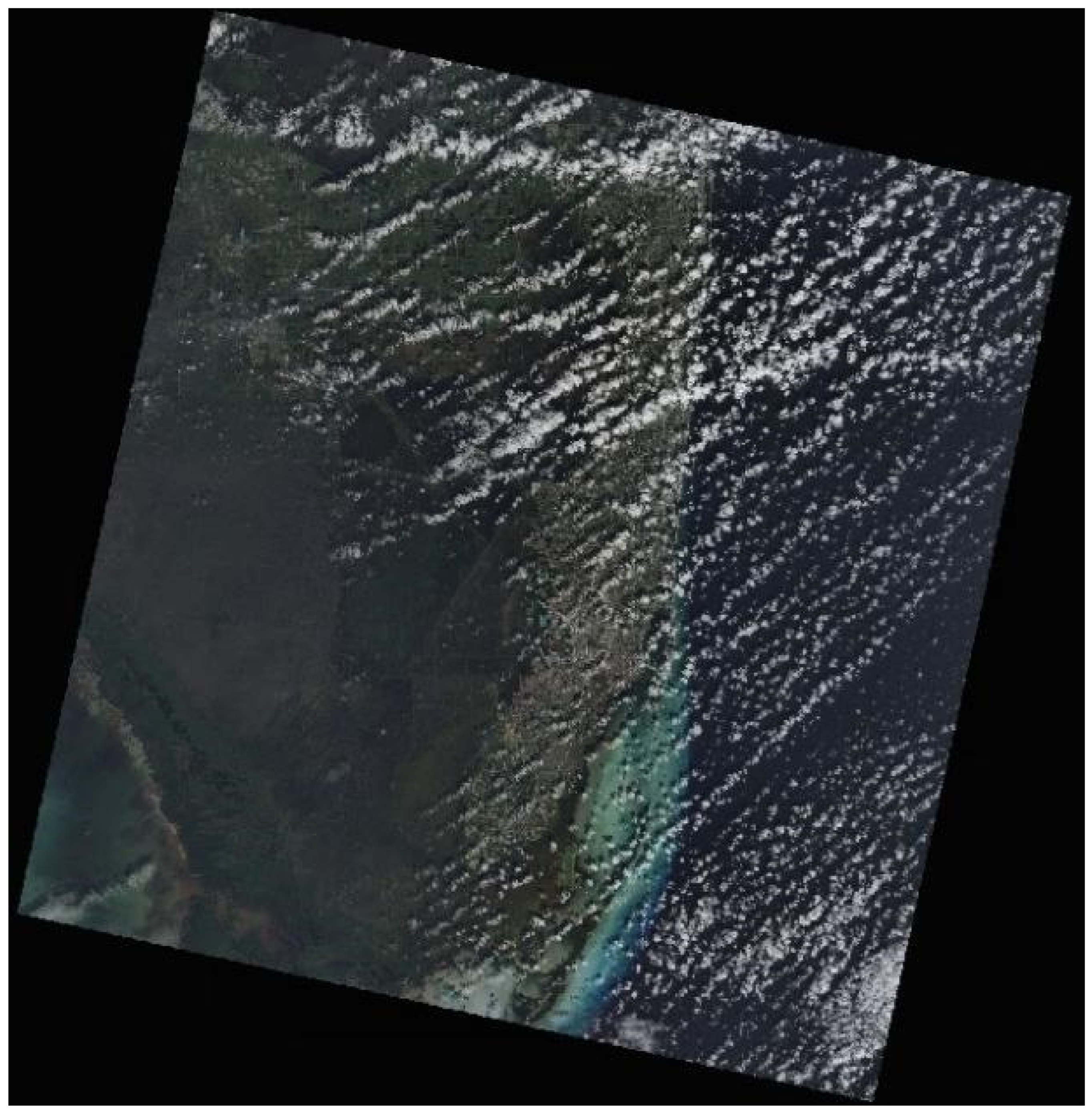
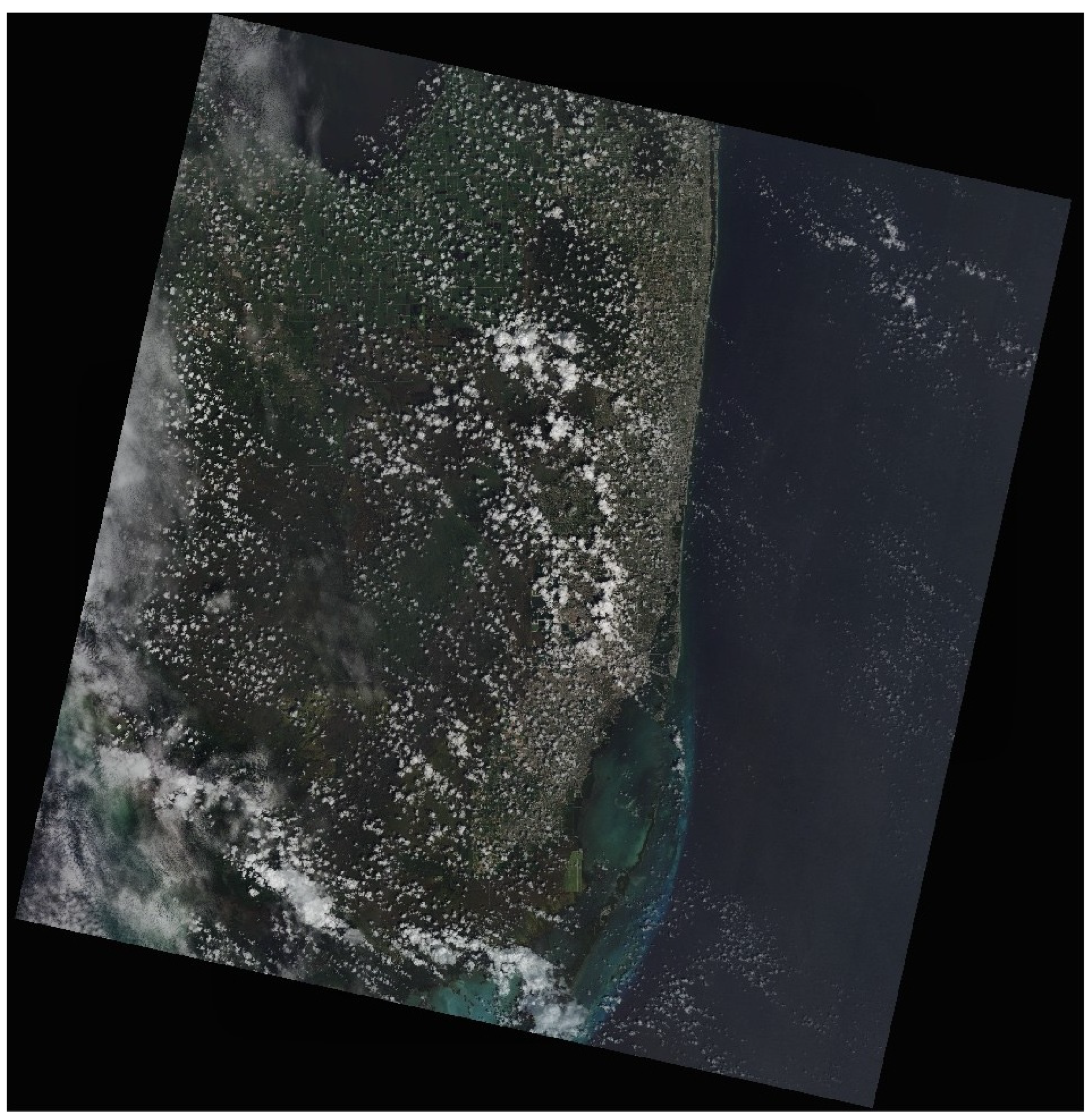
2.1. USGS Landsat-8 Imagery

The first two datasets employed in this study were obtained from the United States Geological Survey (USGS) Landsat Collection Level 1. The selected scenes corresponds to path 15, row 42, with different acquisition dates, encompassing a region in South Florida. This imagery was captured by the Landsat-8 satellite, which is equipped with 11 spectral bands, each corresponding to different segments of the electromagnetic spectrum. These include visible, near-infrared (NIR), shortwave infrared (SWIR), thermal infrared (TIRS) that measure thermal radiation emitted from the Earth’s surface and are used to derive land surface temperature (LST), Cirrus band designed to detect high-altitude cirrus clouds, and a panchromatic band useful for high-resolution mapping and edge detection. The characteristics of these bands are summarized in

Table 1. Landsat-8 Satellite Band Descriptors [15].

Number	Name	Wavelength (µm)	Resolution (m)
1	Coastal	0.430–0.450	30
2	Blue	0.450–0.510	30
3	Green	0.530–0.590	30
4	Red	0.640–0.670	30
5	NIR	0.850–0.880	30
6	SWIR 1	1.570–1.650	30
7	SWIR 2	2.110–2.290	30
8	Pan	0.500–0.680	15
9	Cirrus	1.360–1.380	30
10	TIRS 1	10.600–11.190	100
11	TIRS 2	11.500–12.510	100

.

Upon acquisition, the Landsat-8 imagery is provided as 11 separate GeoTIFF files, each representing a single spectral band. These bands have been merged into a composite data cube using MATLAB R2024a. For visualization, we have utilized the colorize() function from MATLAB’s Hyperspectral Imaging Library for the Image Processing Toolbox, configured with the ContrastStretching parameter set to true. This applies adaptive histogram equalization, enhancing image contrast and producing a false-color RGB composite as shown in Figure 1 and Figure 2.

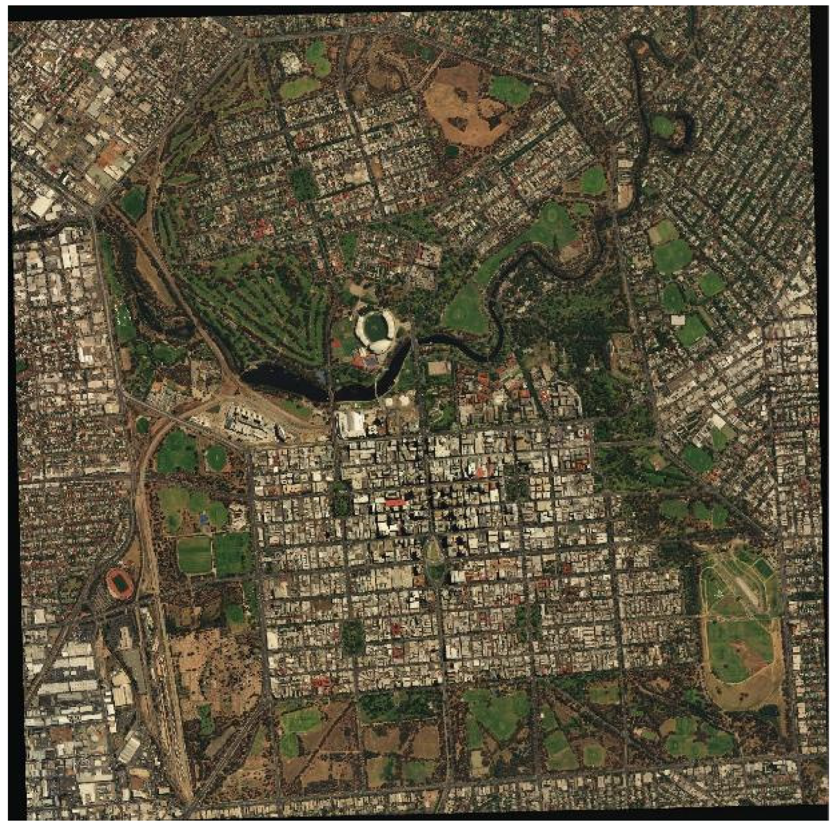
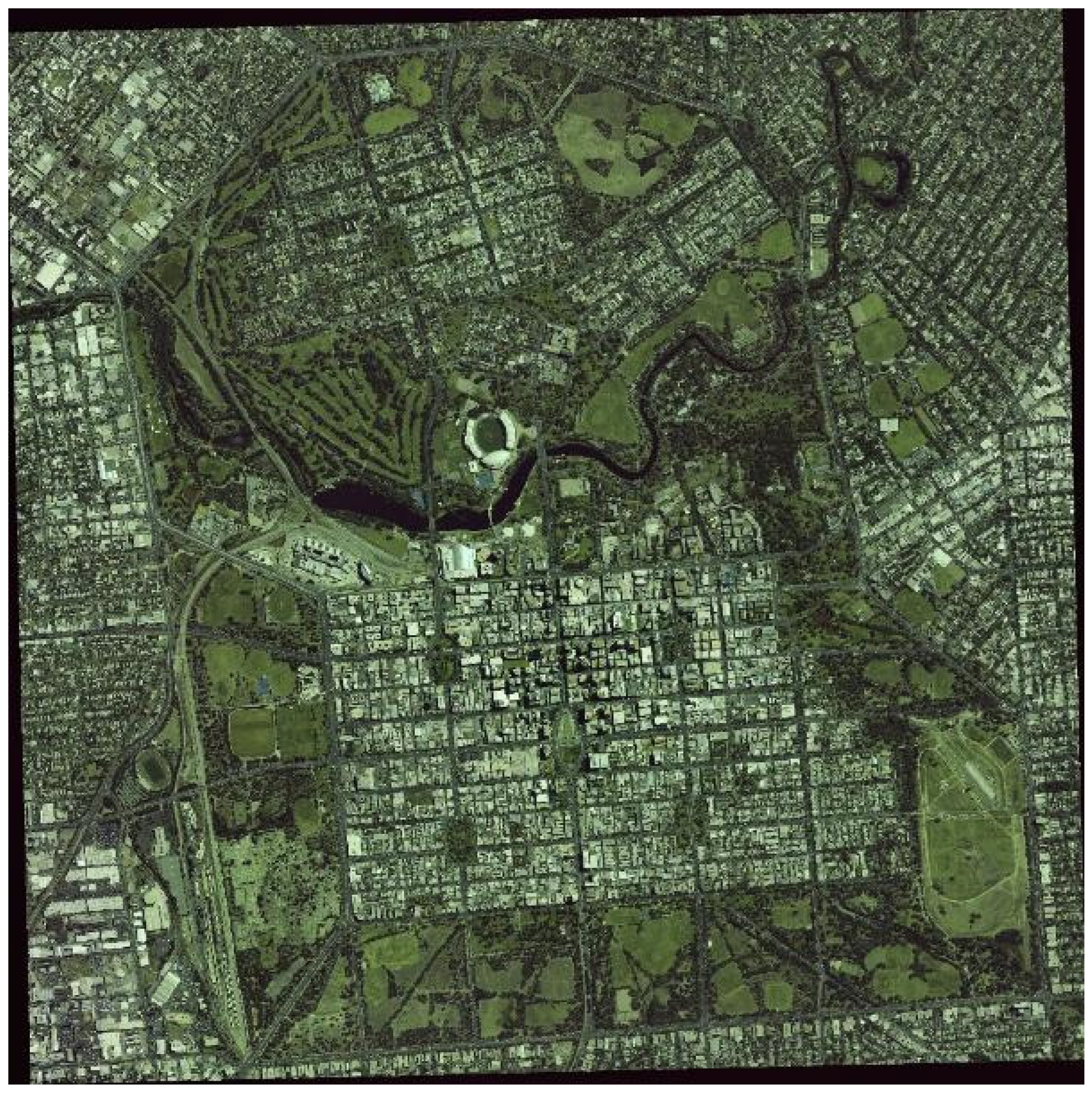
2.2. Apollo Mapping Worldview-3 Imagery

The second dataset utilized in this study was sourced from Apollo Mapping Free Imagery Samples. Although this dataset is freely available for testing, any use beyond experimental or internal purposes requires explicit permission from Apollo Mapping. The image used was captured by the WorldView-3 satellite, which features eight multispectral bands along with a high-resolution panchromatic band. Detailed band specifications are listed in

Table 2. Worldview-3 Satellite Band Descriptors [17].

Number	Name	Wavelength (µm)	Resolution (m)
1	Coastal	0.400–0.450	1.24
2	Blue	0.450–0.510	1.24
3	Green	0.510–0.580	1.24
4	Yellow	0.585–0.625	1.24
5	Red	0.630–0.690	1.24
6	Red Edge	0.705–0.745	1.24
7	NIR 1	0.770–0.895	1.24
8	NIR 2	0.860–1.040	1.24

.

The selected image represents an area over Adelaide, Australia, and is provided as a single stacked file containing all eight spectral bands. As with the Landsat 8 data, the image was processed using MATLAB’s colorize() function with ContrastStretching enabled to generate a visually enhanced RGB composite, presented in Figure 3.

2.3. Independent Component Analysis (ICA) Framework

The primary analytical technique used in this study is Independent Component Analysis (ICA), chosen for its ability to unmix statistically independent sources from mixed signals. When applied to multispectral satellite imagery, ICA can isolate latent spectral components, potentially highlighting geospatial features that are not immediately visible in the raw spectral bands.

Each multispectral image was initially represented as a three-dimensional array X of dimensions (M × N × K), where M and N denote spatial resolution (rows and columns), and K represents the number of spectral bands (e.g., different wavelengths such as red, green, blue, near-infrared, etc.).

Mathematically, X can be visualized as a data cube composed of K two-dimensional spatial layers, each corresponding to a spectral band:

$$\mathrm{X} = \left[\begin{array}{ccc}{X}_{111}& \dots & X_{1N1}\\ ⋮& \ddots & ⋮\\ X_{M11}& \dots & X_{MN1}\end{array}\right]\dots \left[\begin{array}{ccc}{X}_{11K}& \dots & X_{1NK}\\ ⋮& \ddots & ⋮\\ X_{M1K}& \dots & X_{MNK}\end{array}\right]$$

(1)

To prepare the data for ICA, the image cube was reshaped into a two-dimensional matrix X′ as shown in Equation (2) of size (MN × K), where each row corresponds to a pixel’s full spectral signature:

$$\mathrm{X}’ = \left[\begin{array}{ccc}{X\prime }_{11}& \dots & {X\prime }_{1K}\\ ⋮& \ddots & ⋮\\ {X\prime }_{\left(MN\right)1}& \dots & {X\prime }_{\left(MN\right)K}\end{array}\right]$$

(2)

ICA was performed using Python 3.10.12 FastICA() function from scikit-learn version 1.6.1, with a fixed random seed, random_state = 42, to ensure reproducibility. The FastICA algorithm estimates an unmixing matrix W such that the independent components are computed as:

S = WX,

(3)

where W is the unmixing matrix (size n_components × K) that transforms the mixed signals into statistically independent ones, and S is the resulting matrix of independent components, where each column represents a distinct, statistically independent source (e.g., clouds, terrain, water). The scikit-learn is a widely used, open-source machine learning library in Python, and FastICA() is a method provided by scikit-learn for performing Independent Component Analysis on preprocessed multispectral data. These components were then reshaped back into their spatial form (M × N) to produce 2D maps, allowing for visual inspection of each isolated feature distribution.

An inverse transformation can be applied using the pseudoinverse of W, enabling image reconstruction or selective component integration:

X_recon = W⁻¹S

(4)

where X_recon is a reconstructed version of the original data matrix using the independent components. This step allows emphasis or suppression of selected features, such as clouds, waterways, vegetation for refined analysis.

As part of our ablation strategy, to further enhance feature extraction, we performed component subtraction—removing specific ICA components from the original data to reveal subtle residual features (e.g., shadows, surface anomalies) not captured in standard linear reconstructions. Additionally, we applied RGB thresholding to selected components to classify similar spectral regions, supporting tasks such as feature isolation, land-cover discrimination, or cloud delineation. Spatial filtering and morphological post processing was performed in constructing the cloud masks used as ground truth in the different datasets so as to assess the performance metrics of accuracy, precision, recall, Intersection over Union (IoU) and F1 score.

3. Results

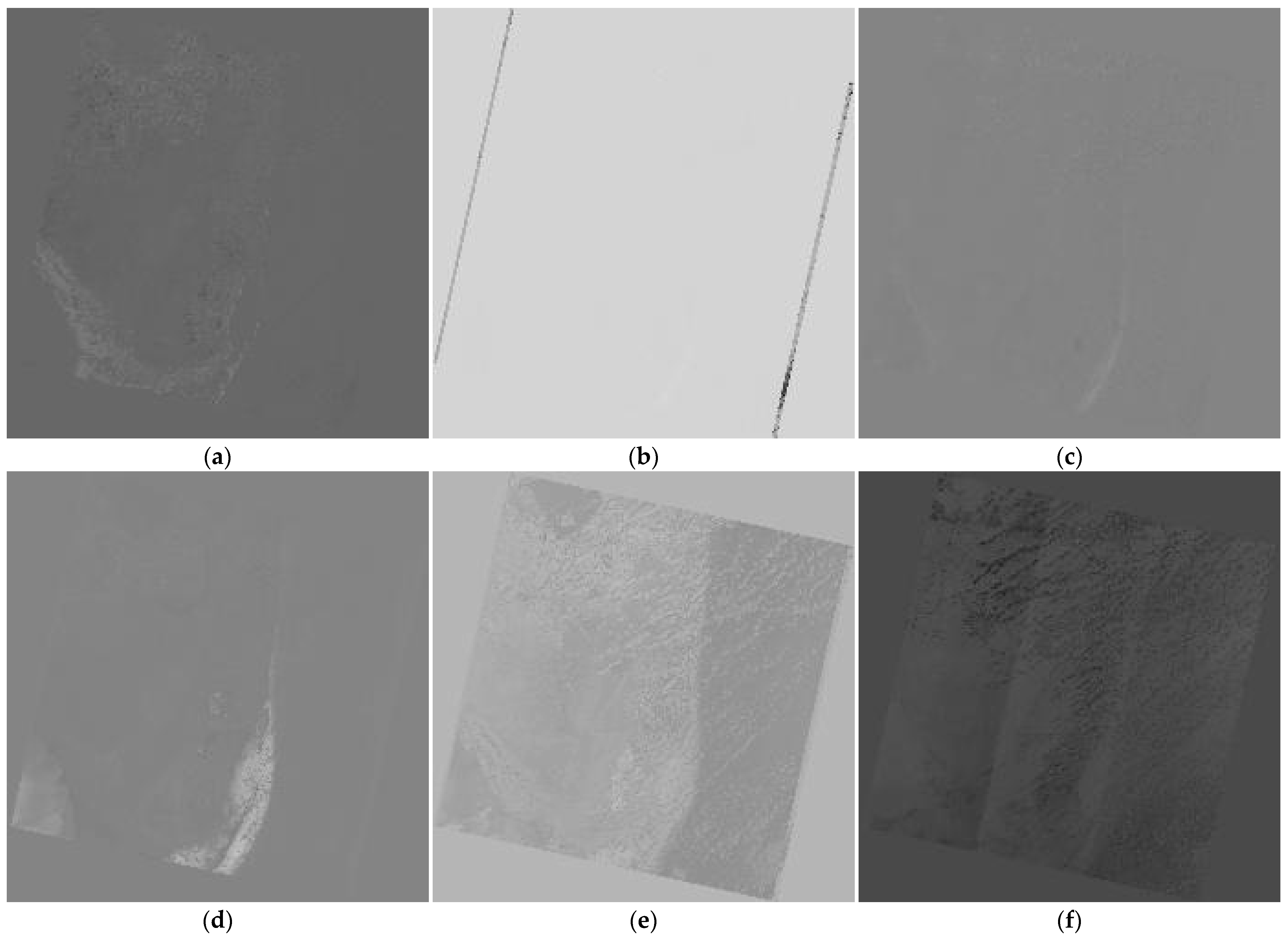
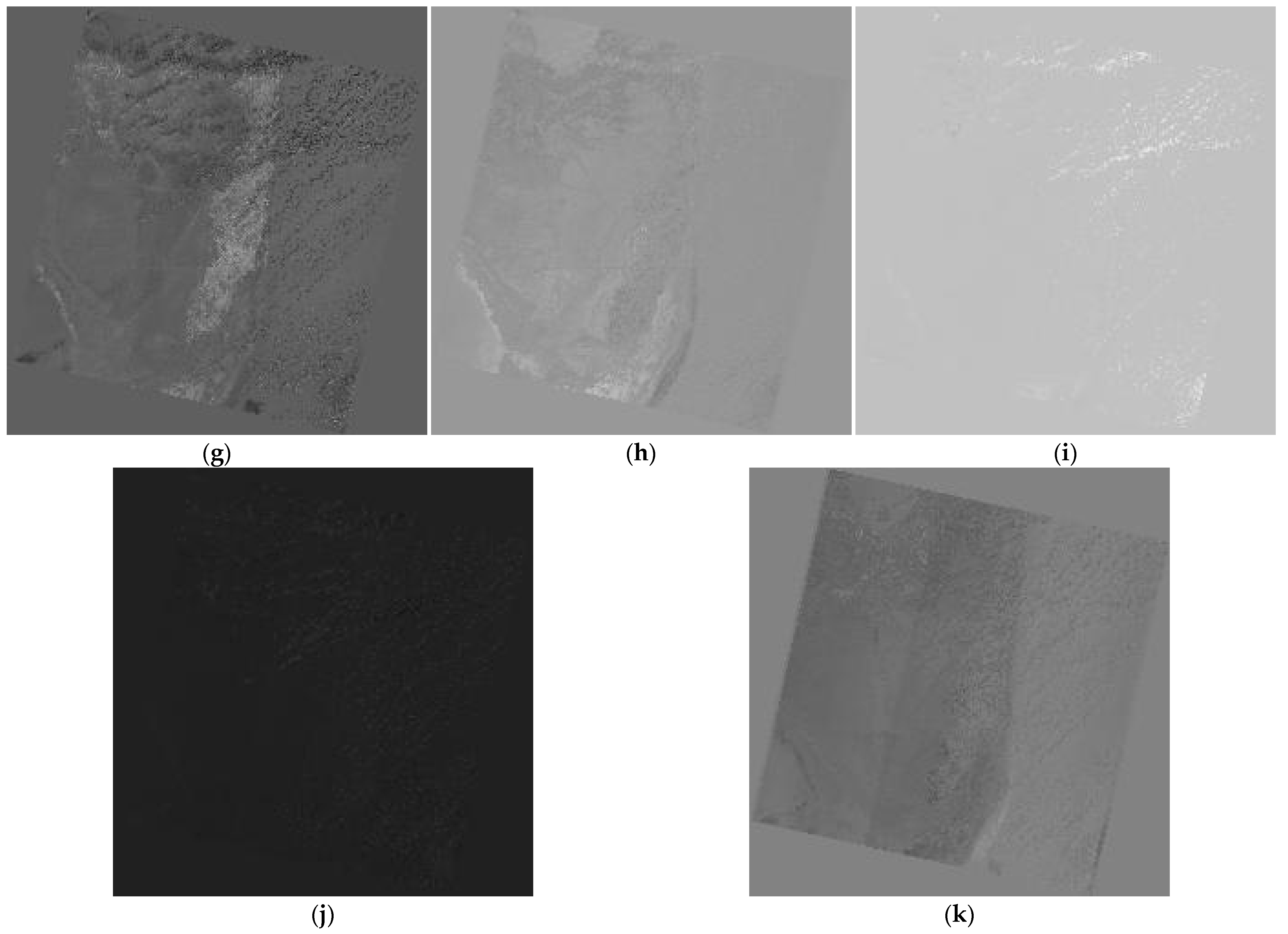
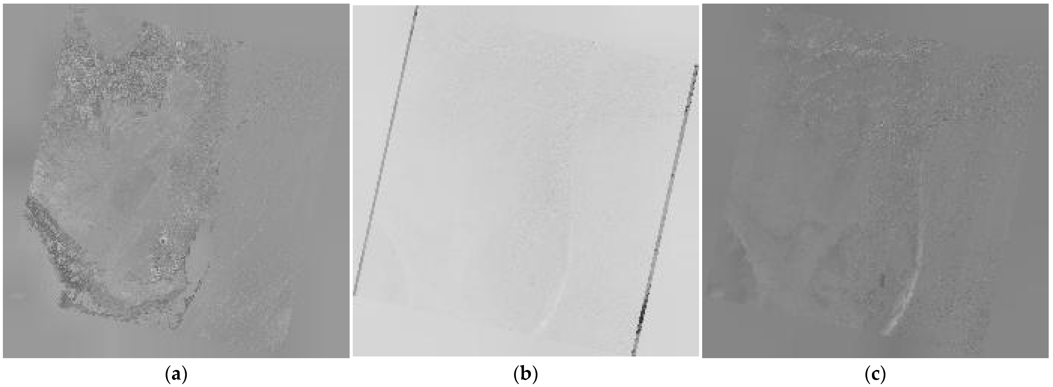
Throughout the text, it is possible to zoom in on the figures for a better appreciation of the results. This is due to the high resolution of the images themselves.

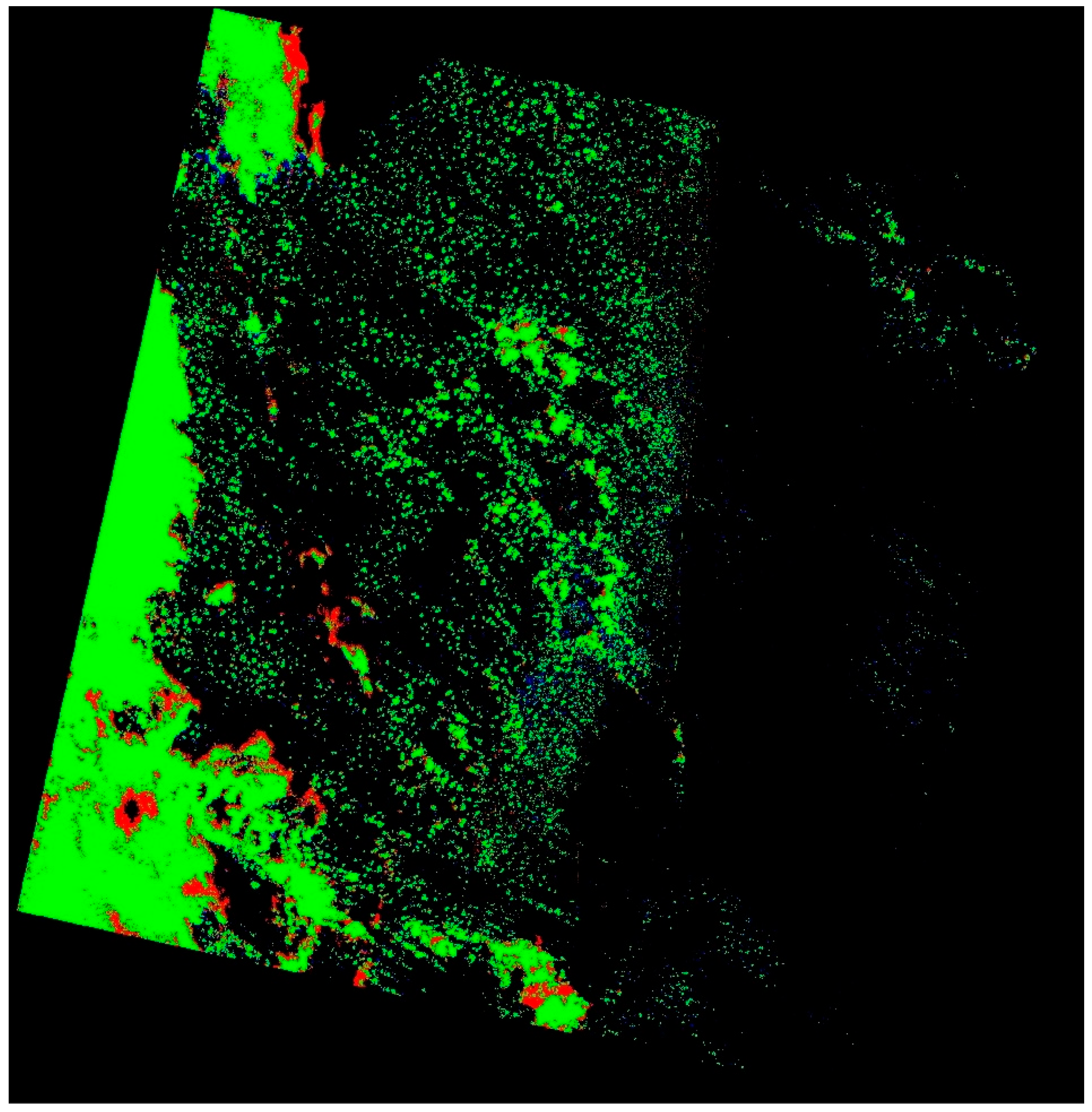
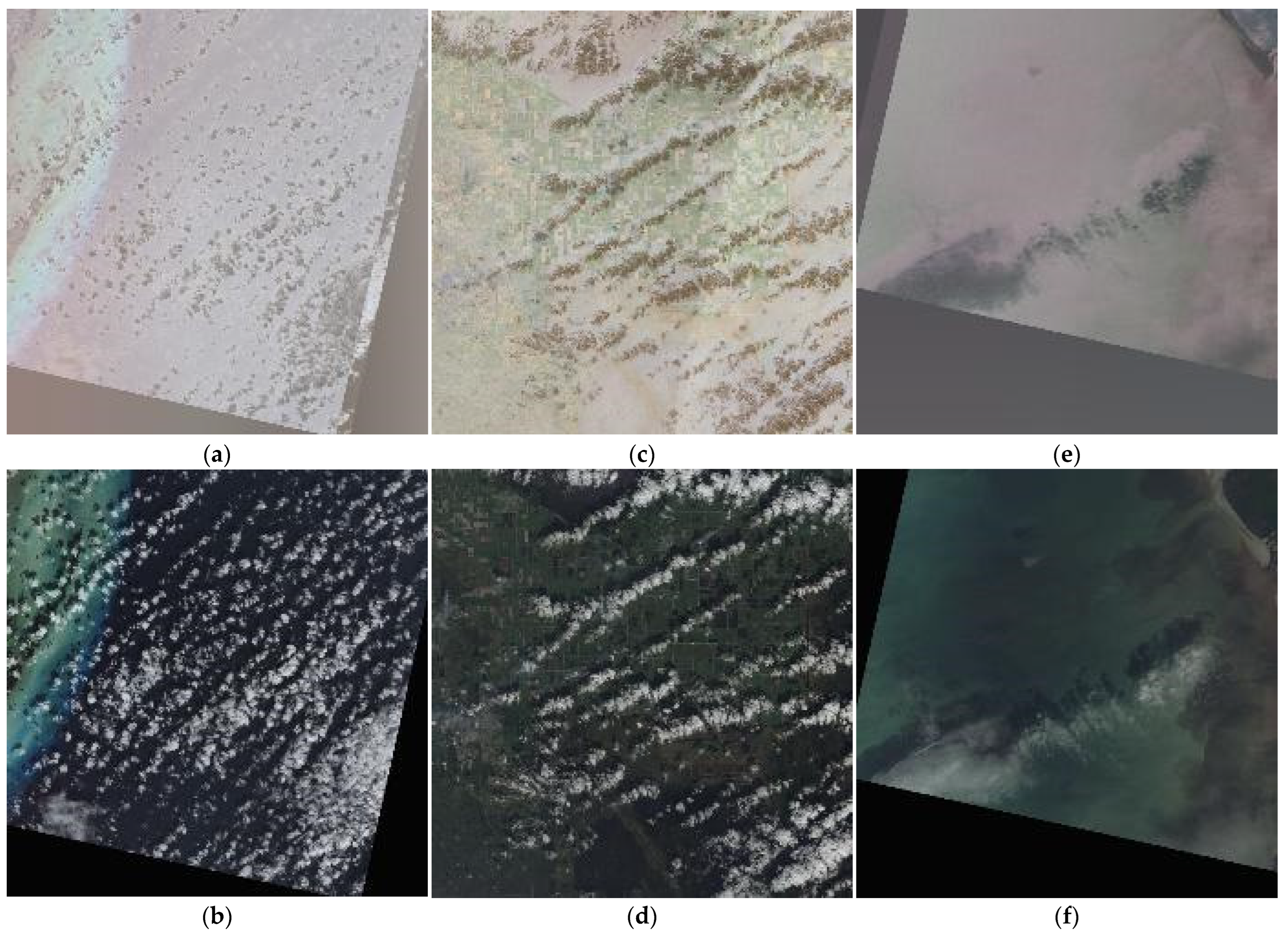
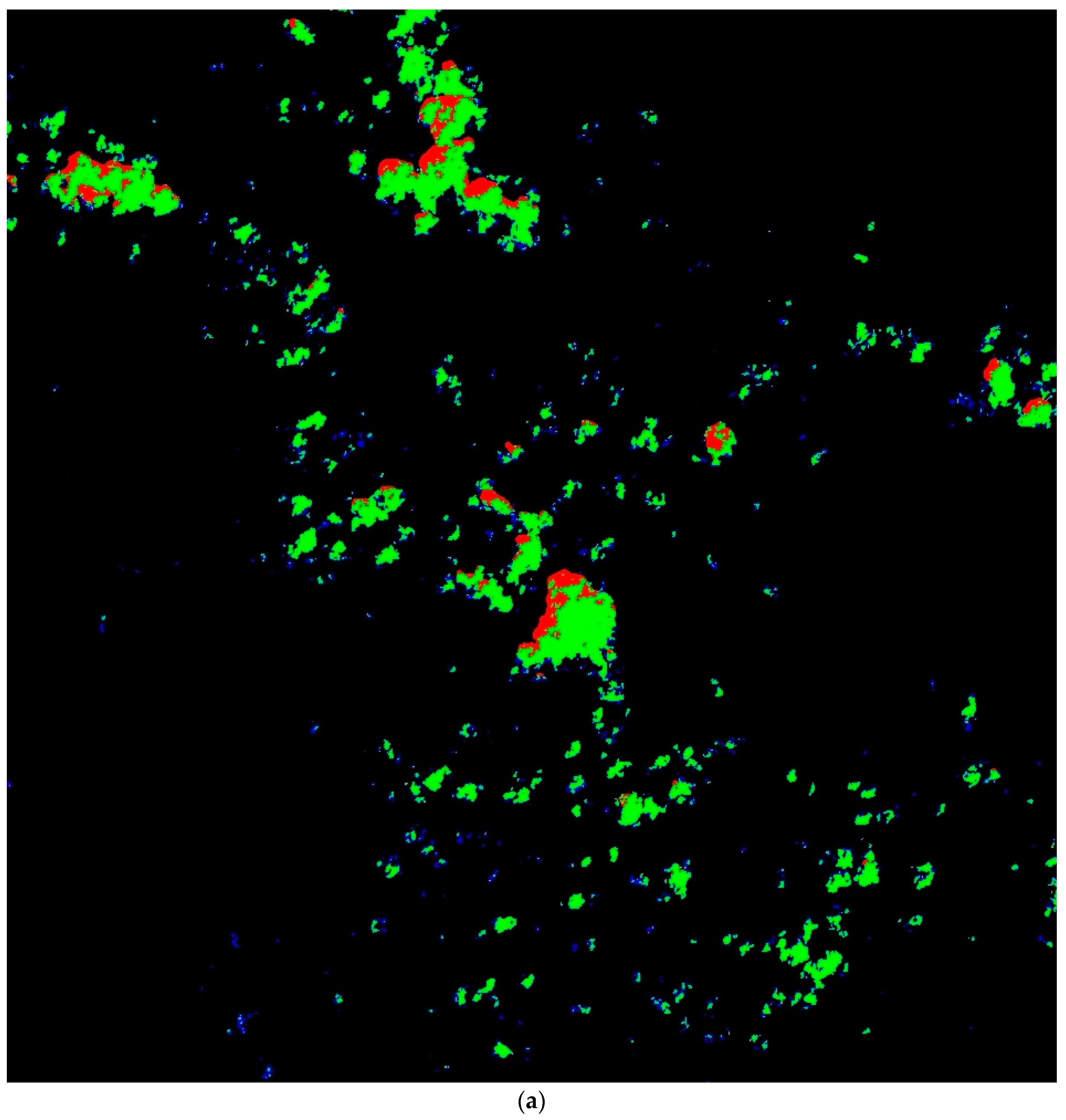
3.1. Landsat-8 Data

The results obtained from applying Independent Component Analysis (ICA) to the Landsat 8 dataset are presented in Figure 4, which displays the individual Independent Components (ICs) extracted from the original multispectral imagery. Visual inspection of these components reveals that certain spatial features are distinctly isolated within specific ICs. For instance, Figure 4d effectively emphasizes shallow water bodies, while Figure 4i distinctly captures the presence of cloud formations concentrated in the top-left quadrant of the image. These findings suggest that ICA is capable of isolating unique spectral sources, such as surface water or atmospheric features, into separate components

Figure 5 illustrates the reconstructed images obtained by projecting the original data using individual ICs. These reconstructions exhibit patterns and enhancements like those observed in the ICs themselves, with some improvements in visual sharpness and spatial feature clarity. For example, Figure 4d,i further emphasize the areas identified earlier as shallow waters and clouds, respectively.

Subsequently, a targeted analysis was conducted to determine if it was possible to isolate and remove cloud-related components with the objective of generating a cloudless or a cloud-reduced image. This procedure involved identifying the IC most closely associated with cloud features and selectively excluding it from the reconstruction process. The intermediate results of this cloud-removal effort are presented in Figure 6. In Figure 6a, the initial removal of the dominant cloud component leads to a partially cloud-cleared image. To further enhance the clarity, a progressive elimination strategy was implemented, whereby additional ICs—suspected of contributing residual cloud artifacts—were removed incrementally. This iterative refinement culminated in Figure 5d, which demonstrates a visually cleaner reconstruction with significantly reduced cloud interference.

The mask generated to serve as ground truth to identify cloud-covered regions in the original image is shown in Figure 7. This mask is used to determine the performance metrics of accuracy, precision, recall, IoU, and F1 Score.

The cloud detection results, as shown in Figure 8, demonstrate the robustness of our ICA-based approach, achieving an overall accuracy of 96.7%, with a precision of 87.4%, recall of 83.2%, IoU of 74.3%, and an F1 score of 89.2%. These high-performance metrics reflect the method’s strong capability to detect clouds with minimal false detections. Notably, many of the observed false positives (highlighted in blue) appear along the peripheries of actual clouds—regions where the ground truth masks may have underrepresented the full spatial extent of cloud coverage. Importantly, our ICA-based reconstruction successfully captured these subtle cloud-contaminated areas, providing a more comprehensive delineation. These discrepancies, while affecting recall and IoU slightly, actually highlight the sensitivity of the method. A closer examination of these boundary regions is presented in the discussion section to clarify their contribution to the overall evaluation.

Building on the results from the original Landsat 8 scene (Figure 1), we extend our evaluation to a newly introduced and significantly more complex aerial dataset, previously presented in Figure 2. This second dataset poses a greater challenge for cloud detection due to its intricate cloud structures, variable terrain features, and the diversity of atmospheric and imaging conditions under which it was captured. As evident in Figure 1 and Figure 2, both datasets cover expansive regions across South Florida, an area known for its dense and heterogeneous cloud formations. The inclusion of this second dataset enables us to rigorously test the generalizability and adaptability of our ICA-based method across different spatial resolutions and sensing contexts.

Following a consistent methodological framework, we begin by reconstructing the second dataset using a targeted subset of Independent Components (ICs 3, 5, 9, and 10), which were empirically determined to isolate cloud-related features most effectively (see Figure 9). To enable quantitative performance evaluation, a ground truth mask delineating cloud-covered areas was generated for this dataset, as illustrated in Figure 10.

The resulting cloud detection performance is presented visually in Figure 11. In this visualization, green pixels denote true positives (cloud regions correctly identified), red pixels indicate false negatives (actual clouds that were missed), and blue pixels represent false positives (non-cloud areas erroneously classified as clouds). These results offer a visual and quantitative demonstration of the method’s capability to adapt to and perform reliably across multispectral datasets of varying complexity.

For this second dataset, the proposed method achieved an accuracy of 97.1%, precision of 92.6%, recall of 86%, IoU of 80.5%, and an F1 score of 89.2% which serve as compelling evidence of the method’s effectiveness and reliability. These results serve as compelling evidence of the method’s robustness and effectiveness in real-world, variable conditions.

Importantly, as will be detailed in the discussion section, many of the false positives (shown in blue) were concentrated along cloud boundaries, areas where the ground truth masks may have underestimated actual cloud coverage, while the false negatives are isolated pixels. Our ICA-based reconstruction effectively captured these transitional cloud regions, reinforcing the algorithm’s sensitivity to subtle spectral variations associated with cloud presence. While this sensitivity slightly impacts recall and IoU, it highlights the method’s ability to detect cloud-contaminated areas that may elude conventional labeling. These regions are further analyzed and discussed in detail in the revised discussion section to provide additional clarity.

Retrospective on Results Across Datasets

The proposed ICA-based cloud detection framework demonstrated strong and consistent performance across two distinct multispectral datasets—an original Landsat 8 scene and a newly introduced, more challenging aerial dataset. On the Landsat 8 dataset (Figure 8), the method achieved an accuracy of 96.7%, precision of 87.4%, recall of 83.2%, IoU of 74.3%, and an F1 score of 89.2%, reflecting a robust capability to delineate cloud-covered regions with low false detection rates. Most false positives (shown in blue) occurred along cloud boundaries, where ground truth masks may have underrepresented the full spatial extent of cloud coverage. Importantly, our ICA-based reconstructions effectively captured these transitional areas, highlighting the algorithm’s sensitivity to subtle spectral variations indicative of cloud presence.

To further evaluate generalizability, we applied the method to a more complex aerial dataset (Figure 2), characterized by intricate cloud structures, diverse terrain, and varying acquisition conditions across South Florida. Using a targeted reconstruction strategy with ICs 3, 5, 9, and 10 (Figure 9), and comparing against a manually generated ground truth mask (Figure 10), the method achieved improved performance: an accuracy of 97.1%, precision of 92.6%, recall of 86%, IoU of 80.5%, and an F1 score of 89.2%. The gains in recall and IoU, in particular, underscore the method’s increased ability to comprehensively detect cloud regions and reduce spatial misclassification, even under complex atmospheric conditions.

As shown in Figure 11, false positives remained concentrated along ambiguous cloud boundaries, while false negatives were predominantly isolated pixels—likely resulting from subtle spectral ambiguity or partial cloud transparency. These localized misses had minimal impact on the global detection accuracy, as the method maintained consistent spatial coherence in cloud segmentation.

Together, these findings affirm the robustness, scalability, and precision of our ICA-based approach across datasets of varying complexity. Detailed analyses of boundary effects, spectral sensitivity, and the nature of misclassifications are further discussed in the revised discussion section to provide additional context and clarity.

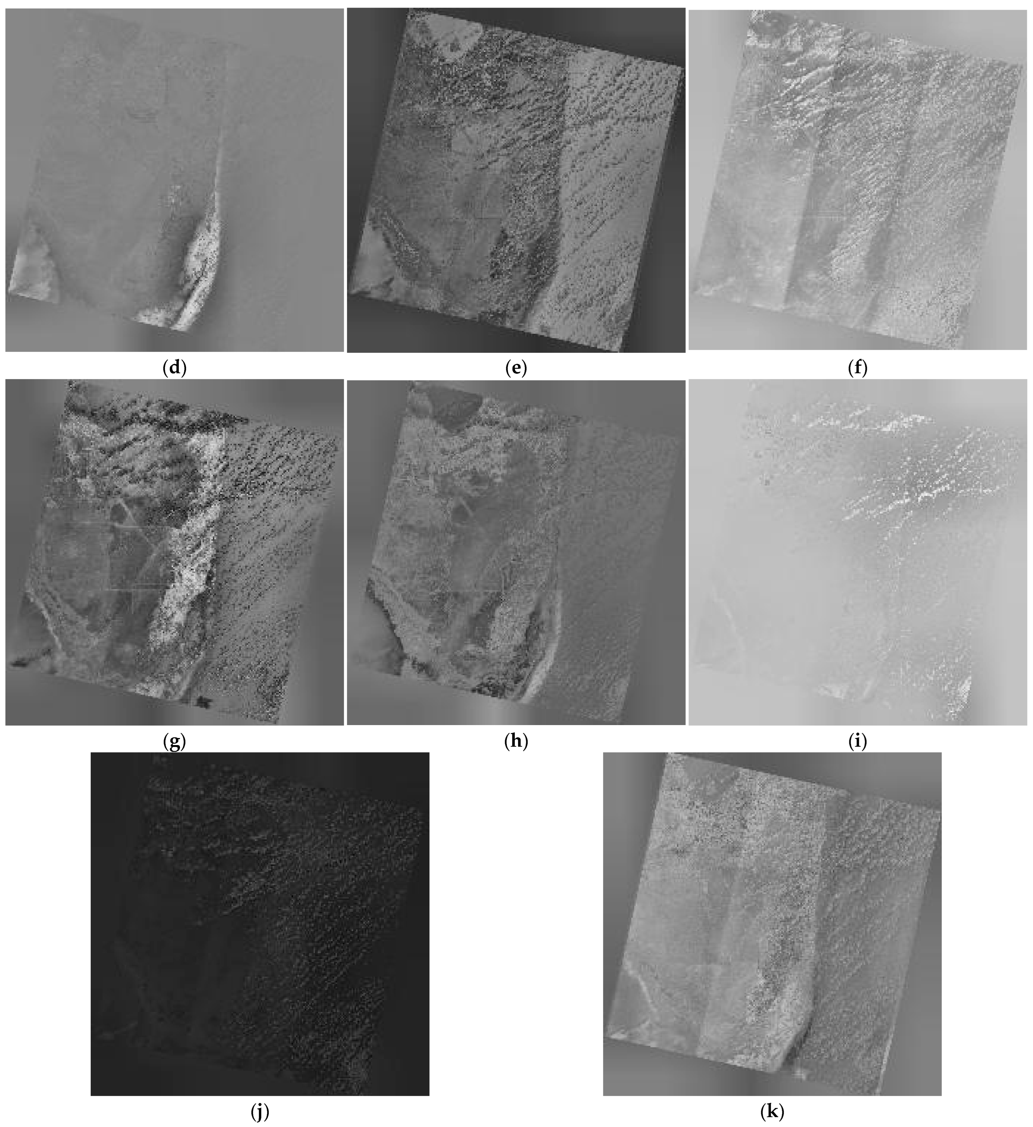
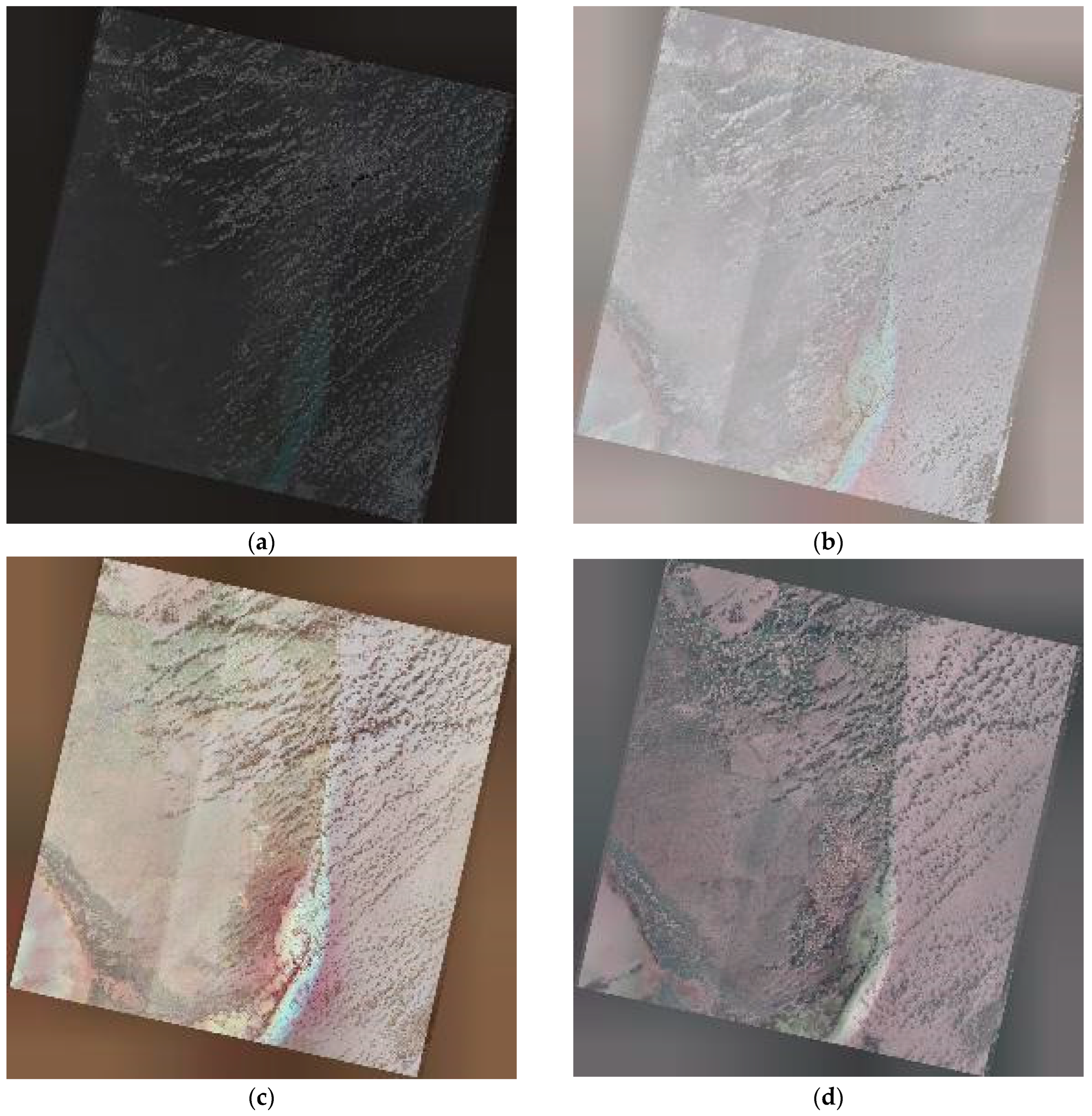
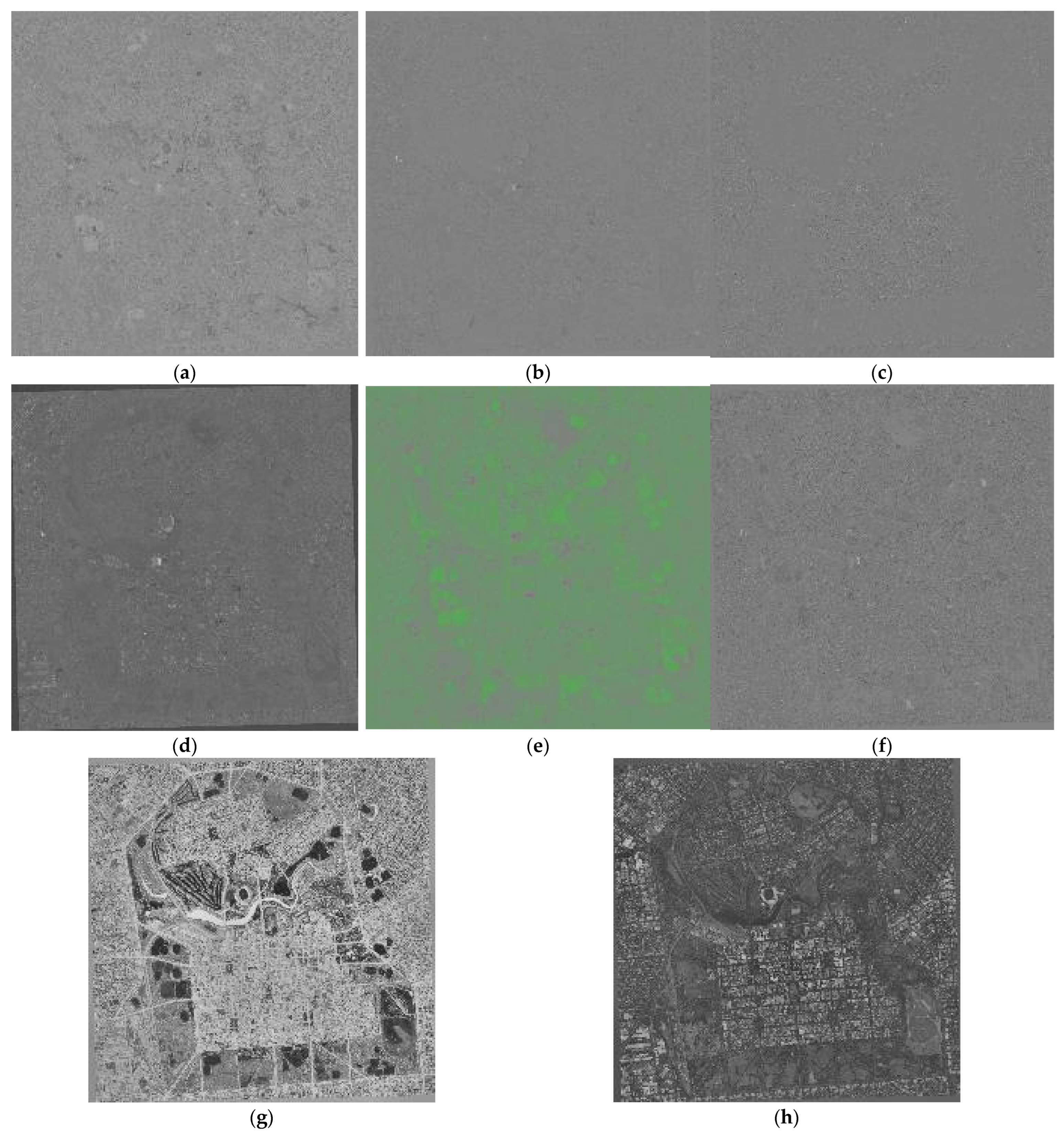
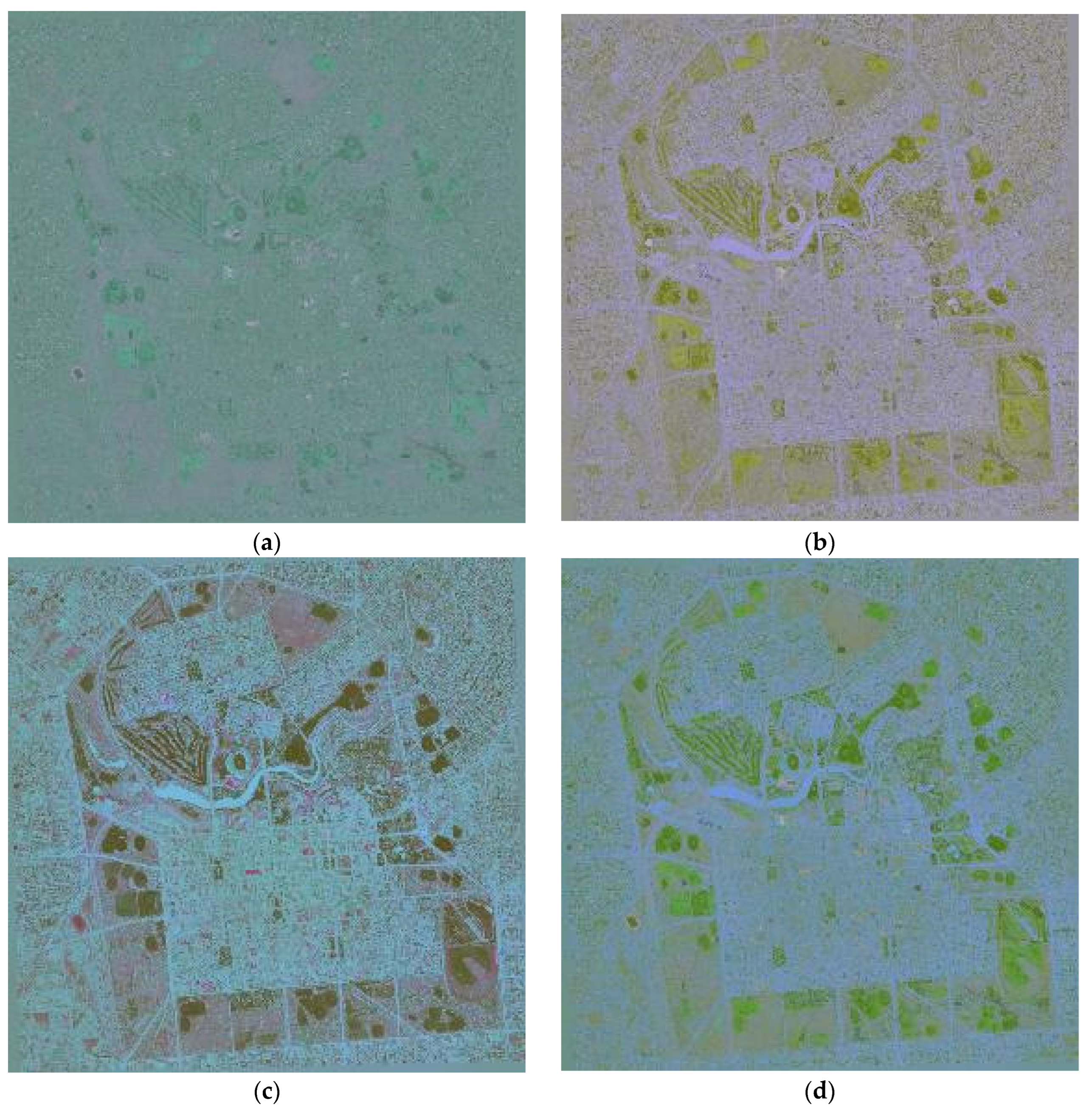
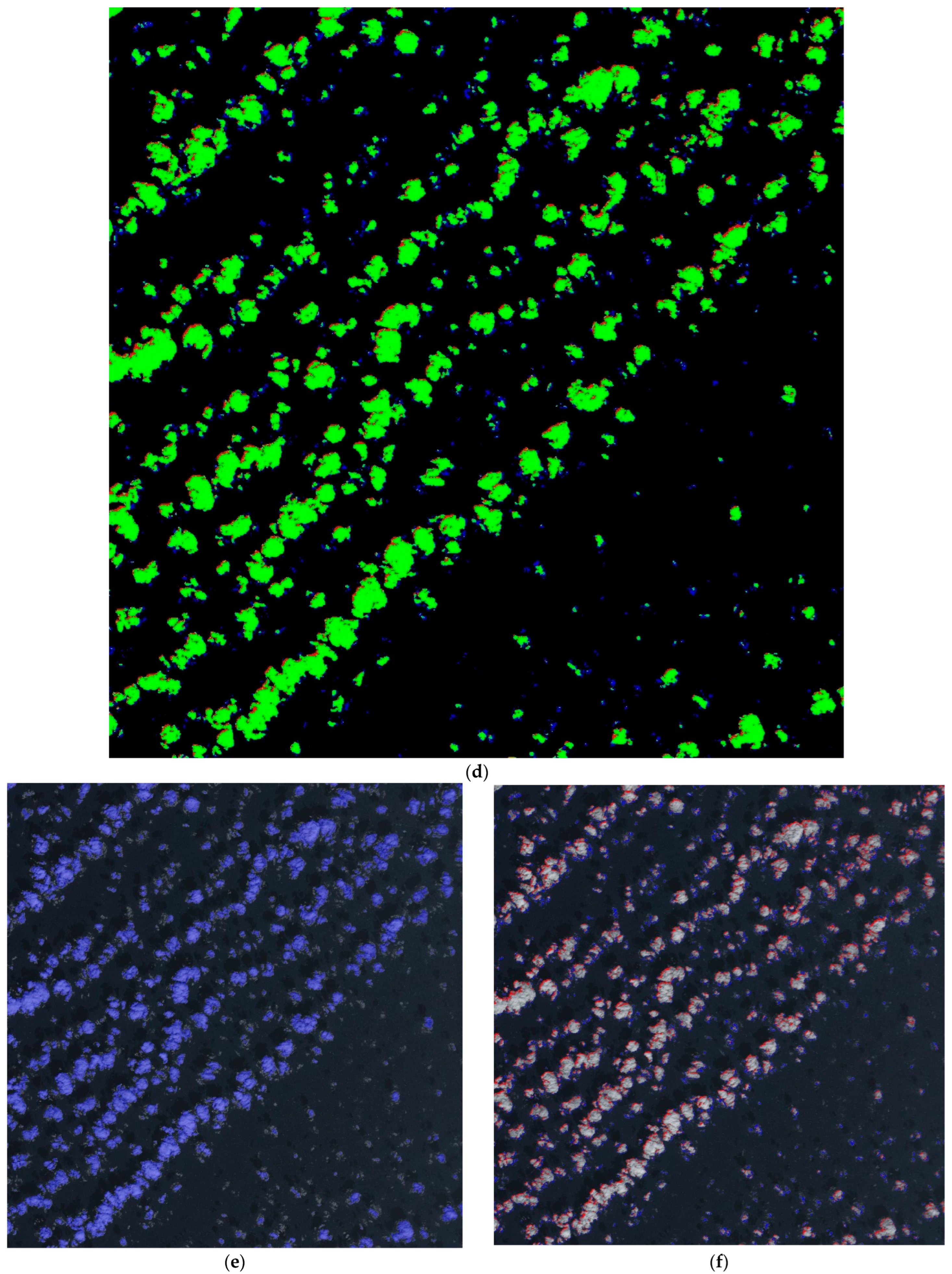
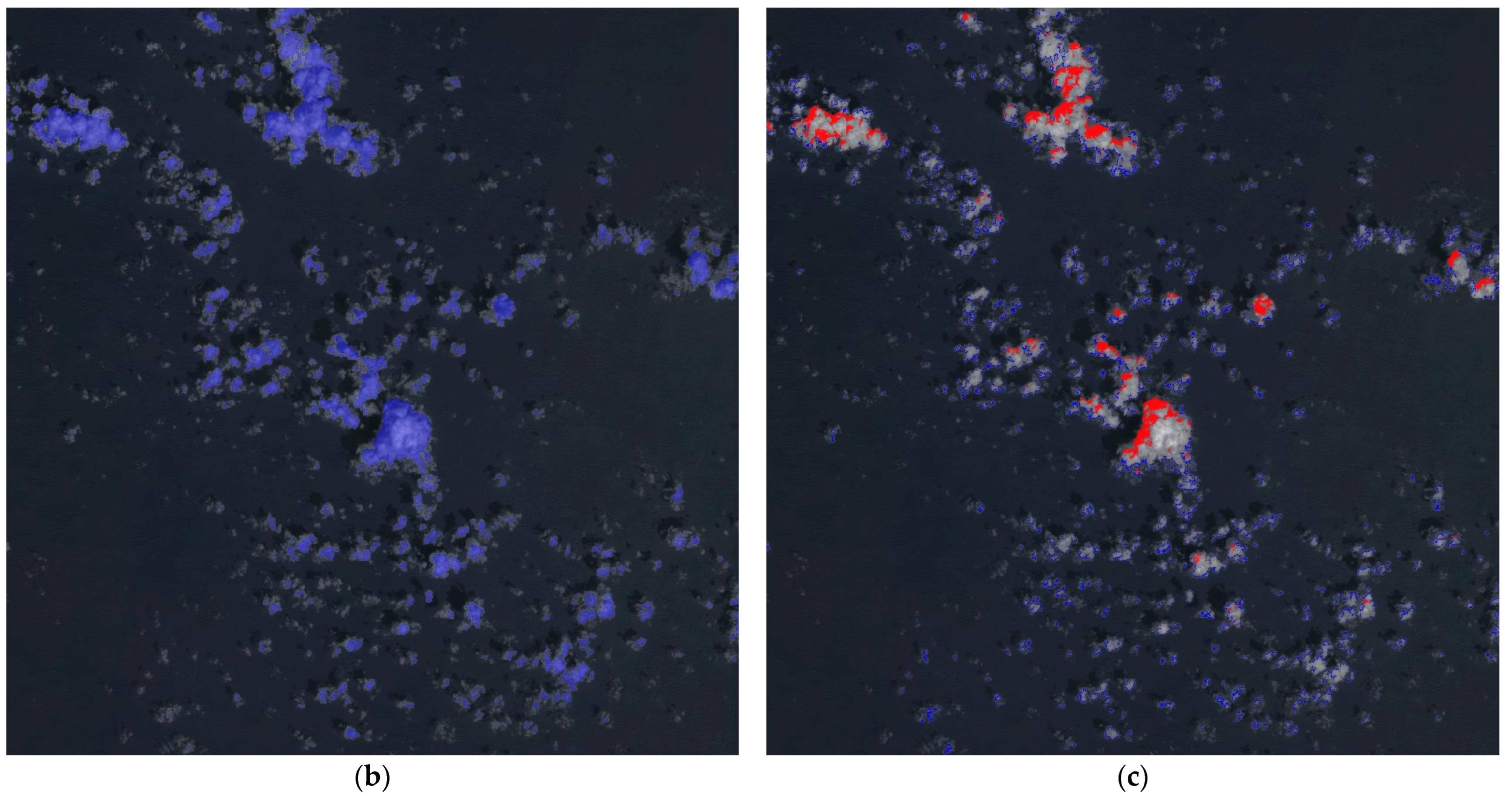
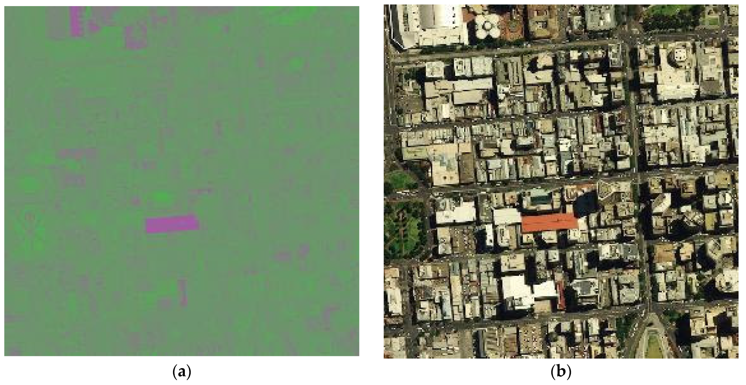
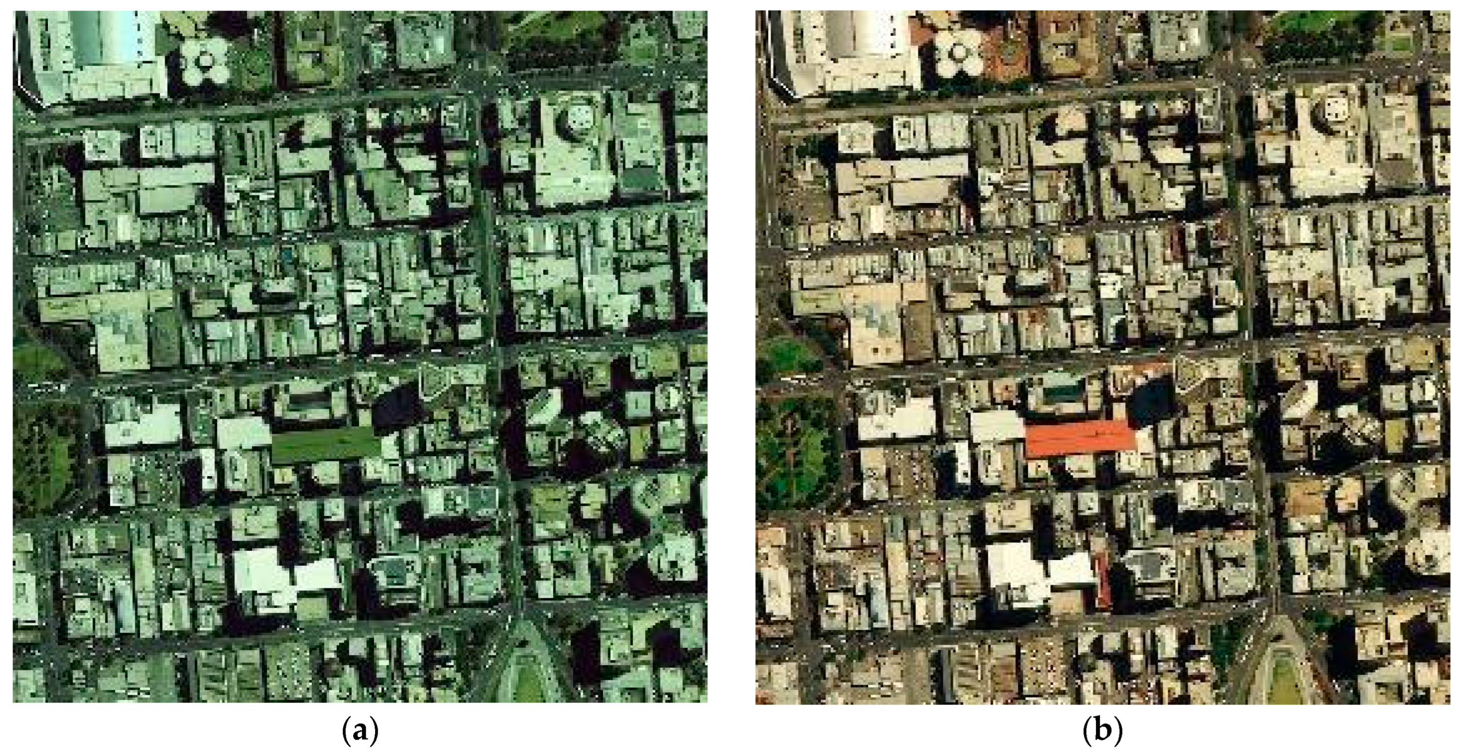
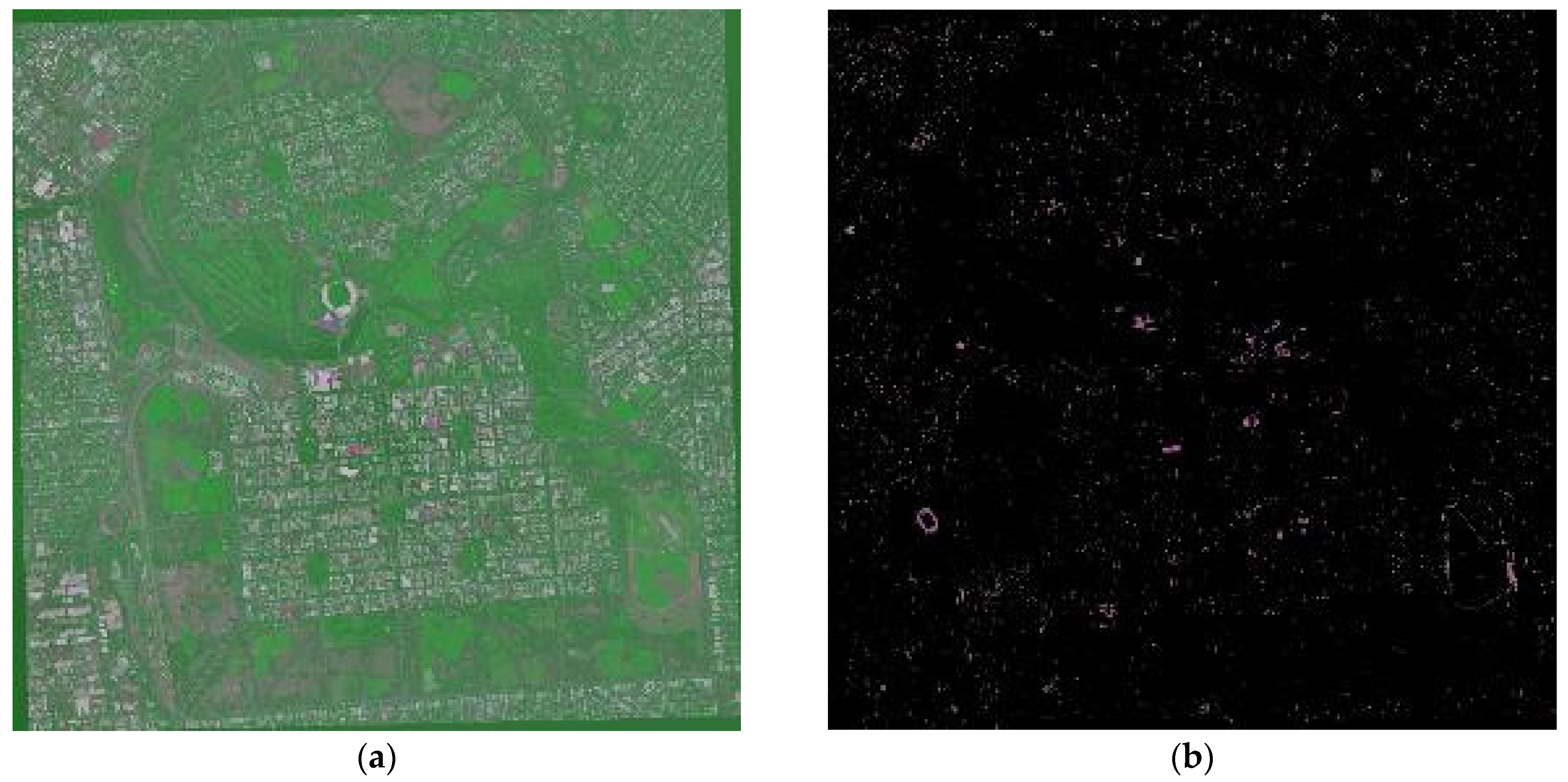
3.2. Results on Worldview-3 Data

The ICA procedure was similarly applied to the WorldView-3 dataset. The resulting Independent Components are shown in Figure 12, which illustrates the decomposed spectral sources obtained from the original imagery. These components exhibit behavior analogous to the Landsat 8 results, particularly in the spatial segregation of ground features. However, due to the absence of prominent cloud formations in this dataset, no IC was found to isolate atmospheric features explicitly.

The reconstruction results using individual ICs are depicted in Figure 13. Most reconstructions, as expected, retained grayscale visualizations consistent with the typical output of ICA. However, Figure 13e stands out as a unique case where the reconstructed image displays enhanced chromatic characteristics, unlike the purely grayscale results observed in other reconstructions. This difference suggests that this particular component may encode a composite or mixed spectral source involving multiple reflectance features.

To further assess the contributions of each IC, a comprehensive set of reconstructions was compiled and is presented in Figure 14. This figure enables a comparative analysis of how each IC influences the visual structure of the image, supporting the interpretation of spectral separation.

Finally, to verify the effectiveness of the ICA decomposition in isolating distinct spectral sources, Figure 15 was generated as a validation figure. This visualization confirms that the ICA successfully separates the original multispectral signal into statistically independent components, which can be used for further analysis and image enhancement, facilitating image segmentation and object identification.

4. Discussion

4.1. Landsat 8 Data

Figure 4 displays all independent components (ICs) extracted via ICA, which were subsequently used to reconstruct the original image and interpret feature behavior. Upon visual inspection, the components reveal identifiable features that suggest associations with specific spectral bands.

Notably, IC4 (Figure 4d) emphasizes areas that appear to correspond to shallow waters. Its corresponding reconstruction in Figure 5d closely resembles the original IC, but with enhanced contrast—brighter white pixels and darker grays—making features more distinguishable. To validate our hypothesis regarding IC4’s sensitivity to shallow waters, we examined two distinct areas in greater detail. Zoomed-in views of both the component and its reconstruction were compared with the corresponding regions in the original image, as can be seen from Figure 16.

Figure 16a–c highlight the southeastern Florida shoreline near North Key Largo and Elliott Key [19], showing clear evidence of coastal waters. Similarly, Figure 16d–f depict salt pools around the CEMEX Doral FEC Aggregates Quarry and White Rock Quarries [20]. In both cases, shallow water features are consistently emphasized in the IC and reconstruction, supporting our interpretation.

With these initial findings, we proceeded to identify components that might represent cloud data, with the aim of removing them to produce a cloud-free image. Visual analysis of Figure 5i shown earlier reveals prominent cloud structures in the top-right corner, which are further examined in Figure 17. The IC9 appears to capture cloud features effectively, as seen in the reconstruction shown in Figure 17a, when compared to the same area in original image as shown in Figure 17b.

Referring back to Figure 6, to explore the potential for cloud removal, we reconstructed the image excluding IC9 and IC2, producing the results shown in Figure 18. In Figure 18a, clouds in some regions were successfully removed, leaving near-zero pixel values. However, Figure 18b demonstrates that residual cloud structures remained, indicating that a single IC does not fully represent all cloud types.

This observation suggests that cloud representation is distributed across multiple components, likely due to varying densities and textures within the clouds themselves. Consequently, we continued the process by progressively removing additional ICs to eliminate more cloud features. Ultimately, removing components IC9, IC2, IC10, IC6, and IC11 resulted in a visibly cleaner image reconstructed from the remaining ICs. Figure 19 illustrates these incremental removals across various sections of the image. In Figure 19, Figure 19a,b show clouds removed from the bottom right after excluding IC10; Figure 19c,d: center clouds eliminated after IC9 was removed; and Figure 19e,f: bottom left clouds removed after excluding IC11. These results highlight the interpretability afforded by ICA in isolating and removing cloud-contaminated features.

Through the process of incrementally removing independent components, we observed that ICA is capable of isolating and delineating cloud structures from other features in the image. However, despite this capability, ICA alone does not allow us to “see through” cloud-covered areas. This limitation arises from the absence of cloud-penetrating spectral data, such as that provided by synthetic aperture radar (SAR) or longer-wavelength infrared sensors. Because traditional optical sensors like Landsat 8 lack these wavelengths, the cloud information remains entangled across several components rather than being isolated in a single IC. As a result, ICA is not well-suited for straightforward, one-step cloud masking. Nevertheless, it remains a powerful tool for high-resolution analysis of cloud morphology and for accurately identifying and extracting the spatial extent of cloud-covered regions. This outcome makes ICA particularly valuable in applications where the goal is to delineate cloud boundaries or mask cloud-affected pixels prior to further analysis, even if it cannot recover the obscured information beneath them.

To gain a deeper understanding of the spatial distribution of false positives (FPs, shown in blue) and false negatives (FNs, shown in red), we present detailed zoomed-in visualizations in Figure 20 and Figure 21. These figures correspond to specific regions within the original input scenes from Figure 1 and Figure 2, respectively, and serve to contextualize the misclassified pixels in relation to the actual cloud structures present in the imagery.

In both Figure 20a and Figure 21a, displays the reconstructed cloud regions superimposed on the ground truth mask offering a visual benchmark against which the reconstruction performance can be assessed. Figure 20b and Figure 21b show an overlay of the ground truth mask over the original image to underscore how specific cloud contours and fine structures, particularly those along cloud edges, are either faintly represented or entirely missing from the annotated ground truth labels. This visual comparison highlights the key limitations of the manual or semi-automated labeling process, particularly when handling thin cloud wisps or small, isolated formations. Figure 20c and Figure 21c highlight the FPs and FNs within these regions, clearly illustrating their spatial alignment relative to actual cloud features. As discussed in the results section, many of the misclassifications occur precisely at the boundaries of true cloud masses. This boundary-level ambiguity is likely a result of underrepresented or imprecise annotations in the constructed cloud masks, which may not fully capture the extent or morphology of diffuse cloud edges. Figure 20d–f are displays of a different example to consider the presence of clouds in both land and sea.

Notably, the ICA-based reconstruction has correctly identified many of these peripheral zones as cloud-contaminated, leading to apparent false positives that may represent legitimate atmospheric features missed by the ground truth. Conversely, some false negatives suggest regions labeled as cloud-free where our reconstruction detected subtle spectral signatures indicative of cloud presence. In several cases, the FPs and FNs consist of sparsely distributed or single-pixel anomalies—common in complex, high-resolution imagery—making definitive classification inherently challenging.

Together, these zoomed-in analyses support the argument that some discrepancies between prediction and annotation are not necessarily errors in reconstruction, but rather artifacts of incomplete or subjective ground truth labeling, particularly in transitional zones where cloud presence is ambiguous or visually subtle.

This detailed inspection highlights the precision of our method in identifying subtle cloud structures and reveals that many classification discrepancies are due to ground truth limitations rather than algorithmic errors.

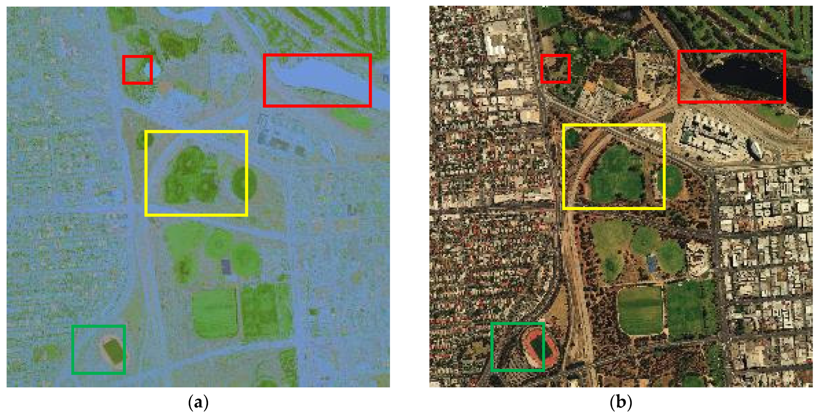
4.2. Analysis on Worldview-3 Data

Looking back at Figure 13, one of the reconstructed images stands out due to its green and pink coloration (Figure 13e) rather than grayscale (Figure 13a–d,f–h). Zooming into these regions, we observe that pink areas correlate with red features in the original image, such as rooftops and red-colored buildings and vehicles that are so small given the resolution at hand that would have otherwise never been detected. This observation suggests that IC5 represents the red spectral band, which is supported by the comparison in the results shown in Figure 22.

To confirm this, we reconstructed the image excluding IC5, as shown earlier in Figure 15. Comparing the results with the original image shown in Figure 23b, the previously red features now appear green as shown in Figure 23a, validating our hypothesis regarding IC5’s contribution to the red band.

In addition to this band isolation, we explored combinations of other ICs to analyze how their integration influenced image reconstruction. Referring back to Figure 14, which presented different combinations of ICs, with notable results arising from merging IC1 with IC5. This produced an image where red areas appeared pink, albeit with reduced color intensity elsewhere.

We then combined IC1 with IC7, which seemed to suppress vegetation features (lower pixel values) while enhancing water bodies. This resulted in a reconstruction that clearly highlighted vegetation in green. Finally, combining IC1, IC5, and IC7 yielded a well-balanced image as shown in Figure 24, accurately capturing red roofs, and running track in a stadium, green vegetation, and water bodies, all in hues corresponding to their real-world counterparts. Highlighting different sections with different colors, the results show:

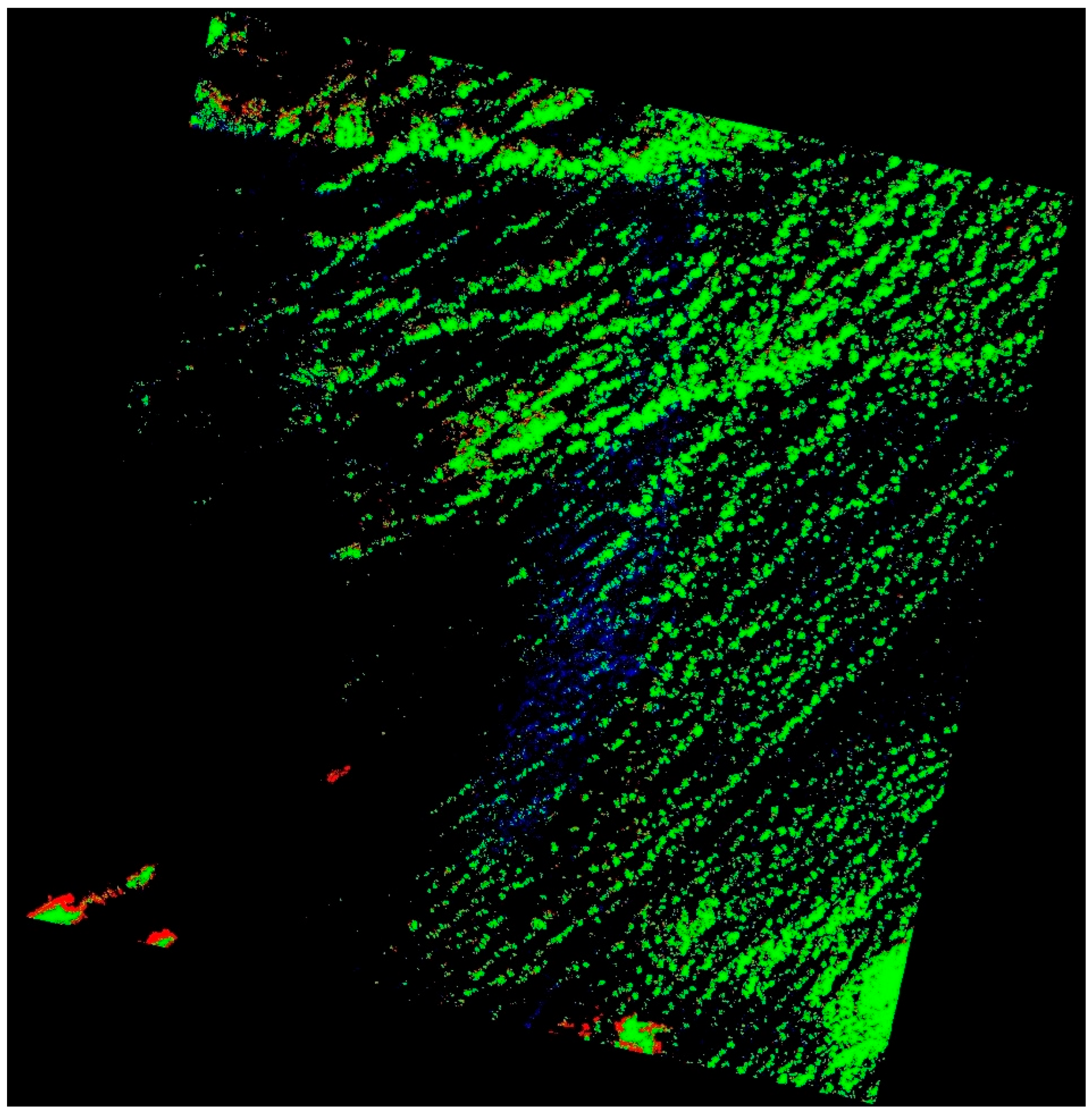
• Yellow boxes: Grassy regions retained green color tones in both the original and reconstructed images.
• Green box: A red track remained distinguishable from adjacent grassy areas.
• Red boxes: Ponds and water bodies were correctly identified, even when their visual appearance mimicked grassy fields, demonstrating ICA’s ability to capture latent spectral distinctions.

Another promising approach emerged from experimenting with subtraction. In Figure 25, subtracting reconstructions yielded visuals similar to those obtained via ICA. By isolating red pixels using RGB thresholds derived from IC5, we generated a binary image highlighting all red features (rooftops, red-colored cars, reddish land patches, and dirt), as shown in Figure 25b.

We extended this subtraction technique to another reconstruction that omitted IC7. Although it introduced confusion between water and grayish infrastructure (e.g., streets and roads), thresholding still successfully isolated water features as shown in Figure 26b. This type of subtraction with appropriate RGB thresholding represents a useful preprocessing step for minimizing feature ambiguity and optimizing feature extraction and segmentation.

This thresholding and subtraction technique holds potential for longitudinal studies, where isolating and tracking specific features across time could aid in change detection or environmental monitoring.

5. ICA-Based Cloud Detection Within the Remote Sensing Landscape

Cloud detection in satellite imagery remains a fundamental challenge in remote sensing, especially across heterogeneous terrains, sensors, and atmospheric conditions. While recent advances in deep learning—such as Conditional GANs [21], U-Net variants [22], and feature pyramid networks [23]—have improved segmentation and cloud removal, these methods often depend on large and labeled datasets and still struggle with generalization and synthetic fidelity. In contrast, Independent Component Analysis (ICA) offers a powerful, unsupervised alternative grounded in statistical source separation. It excels at isolating cloud-related signals from multispectral and hyperspectral imagery without requiring model pretraining, dense training data, or physical assumptions.

Several recent studies support the utility of unsupervised methods in isolating clutter or clouds. Shi et al. [24] demonstrated that combining K-means clustering with dynamic thresholding improves the clarity of atmospheric signals in radar data. Similarly, Nguyen et al. [25] employed unsupervised filtering to segment volumetric noise in LiDAR point clouds. These works echo our ICA approach, emphasizing the value of statistical segmentation when labeled data are scarce.

Prades et al. [26] further validate the power of ICA in hyperspectral unmixing, where it outperformed traditional metrics by isolating complex, independent material signatures, reinforcing ICA’s suitability for spectral decomposition. Zhu et al. [27] highlighted the challenges in subpixel snow mapping due to the limited availability of cloud reference data, underscoring the need for methods like ICA that can bypass such constraints. Liu et al. [28] integrated ICA with InSAR time-series to separate atmospheric noise from deformation signals during the 2023 Turkey–Syria earthquakes, achieving a 43.08% improvement over MSBAS and confirming ICA’s precision in geophysical signal retrieval.

From a multispectral segmentation perspective, Huang et al. [23] demonstrated that incorporating SWIR bands significantly enhances CNN performance, provided that well-structured networks, such as FPNs with residuals, support it. In contrast, ICA remains model-agnostic and requires no architectural tuning. Similarly, Jeppesen et al. [22] RS-Net depends on labeled training across varied conditions—something ICA circumvents through direct statistical decomposition.

Foundational efforts, such as those by King et al. [29], laid the groundwork for cloud retrieval using MODIS; however, their reliance on fixed models and limited resolution constrains performance in complex environments. ICA introduces flexibility and statistical adaptability, enabling better extraction even from low-resolution or noisy data. Claverie et al. [30] improved the harmonization of Landsat-8 and Sentinel-2 data through HLS preprocessing; however, residual cloud artifacts remain a gap that ICA can help fill by unsupervised component separation.

Kussul et al. [31] achieved high classification accuracy using supervised CNN and MLP models with cloud restoration steps. Our ICA approach complements this pipeline, offering fast and interpretable preprocessing, particularly useful in data-limited settings. Meanwhile, Meraner et al. [32] SAR-optical fusion for cloud removal highlights how inference-based reconstructions, while visually plausible, may fail to preserve spectral integrity. ICA, by contrast, works directly on observed data, retaining its physical authenticity.

Li et al. [33] provide a comprehensive review of cloud detection algorithms, ranging from rule-based to deep learning, highlighting the challenges of generalizing across various platforms and conditions. Our ICA-based framework directly addresses this challenge, offering robust performance without relying on training or physical models.

In retrospect, this review of the remote sensing landscape illustrates a persistent need for scalable, interpretable, and generalizable cloud detection methods. Our ICA-based approach directly addresses these issues by separating statistically independent cloud components in a model-free and unsupervised manner. As deep learning models become increasingly complex, we advocate for hybrid architectures that combine the interpretability of ICA with transformer-based learning for more adaptive and robust cloud processing pipelines. Ultimately, while GAN-based reconstructions [21] offer visual realism, ICA stands out for its mathematical rigor, adaptability to diverse conditions, and minimal data dependency. A hybrid future where ICA, paired with SAR, SWIR, and attention-based networks, promises to advance cloud detection for real-time, resilient remote sensing workflows.

6. Conclusions

This study demonstrates the utility and limitations of Independent Component Analysis (ICA) as a tool for spectral source separation in multispectral imagery affected by clouds and shadows. Using datasets from both Landsat 8 and WorldView-3, we observed that ICA is capable of isolating certain atmospheric and surface features into distinct components. In the case of the Landsat-8 data, ICA has enabled the partial extraction of cloud-related components and facilitated the delineation of clouds. This was achieved by systematically identifying and removing multiple independent components that encoded cloud information, although it required a multistep approach due to the spectral complexity and density variation within cloud formations.

In contrast, the WorldView-3 dataset, which contained minimal cloud interference, served to validate ICA’s potential for isolating other spectral features. Notably, components associated with specific colors, such as red rooftops and vehicles, were effectively extracted, demonstrating ICA’s applicability beyond cloud analysis for tasks such as urban feature identification, segmentation, and object classification.

ICA does not inherently differentiate cloud data into a single component, and separating complex obstructions like semi-transparent clouds or shadows often necessitates the removal of multiple components, potentially at the cost of losing relevant land surface information. This suggests that ICA, while powerful, may be best employed as a complementary technique rather than a standalone solution for atmospheric correction.

Future work could enhance ICA’s effectiveness by integrating it with multi-sensor fusion, spatial context modeling, or supervised classification techniques to refine the identification of atmospheric features. Additionally, a more targeted band selection or the use of shortwave infrared and thermal bands may improve cloud discrimination. Overall, ICA remains a valuable tool for feature extraction and exploratory analysis in multispectral remote sensing. One thing is for sure: traditional image processing techniques would not be able to segment the image in the way ICA could.

In retrospect, while ICA’s reliance on statistical independence does limit its ability to directly reconstruct obscured information, such as what lies beneath dense clouds, it nonetheless offers a powerful preprocessing step for feature extraction of key elements and objects present in these multispectral images. Although it is demonstrated that clouds could be delineated through key principal components, future improvements must include spectral wavebands such as SAR that can penetrate clouds. As a practical interim solution, once cloud surfaces are delineated, corresponding regions can be visually explored through alternative platforms, such as Google Maps, to determine and identify the obscured ground features. Another potential solution could be explored with the use of data from different satellites, like Sentinel-2, which has expanded 13 spectral bands with varying resolutions [32]. Upon obtaining data from this satellite, we could implement similar methodologies, as well as combine them with SAR, for possibly improved results.

Looking ahead, we envision combining ICA with advanced machine learning or deep learning models and integrating data from additional sensors with narrower spectral bands when available. These enhancements hold the potential not only to improve ICA’s delineation of clouds and the shadows they cast but also to extract nuanced and intersecting features from increasingly complex remote sensing environments.

References

- Cagnazzo, M.; Poggi, G.; Verdoliva, L. Region-based transform coding of multispectral images. IEEE Trans. Image Process. 2007, 16, 2916–2926. [Google Scholar] [CrossRef]
- Torres, J.; Vazquez, D.; Antelo, T.; Menendez, J.M.; Posse, A.; Alvarez, A.; Munoz, J.; Vega, C.; Del Egido, M. Acquisition and formation of multispectral images of paintings. Opt. Pura Apl. 2012, 45, 201–207. [Google Scholar] [CrossRef]
- Ma, Z.; Ng, M.K. Multispectral Image Restoration by Generalized Opponent Transformation Total Variation. SIAM J. Imaging Sci. 2025, 18, 246–279. [Google Scholar] [CrossRef]
- Wang, Z.; Zhou, D.; Li, X.; Zhu, L.; Gong, H.; Ke, Y. Virtual image-based cloud removal for Landsat images. GISci. Remote Sens. 2023, 60, 2160411. [Google Scholar] [CrossRef]
- Tong, Q.; Wang, L.; Dai, Q.; Zheng, C.; Zhou, F. Enhanced cloud removal via temporal U-Net and cloud cover evolution simulation. Sci. Rep. 2025, 15, 4544. [Google Scholar] [CrossRef]
- Ma, D.; Wu, R.; Xiao, D.; Sui, B. Cloud Removal from Satellite Images Using a Deep Learning Model with the Cloud-Matting Method. Remote Sens. 2023, 15, 904. [Google Scholar] [CrossRef]
- Han, J.; Zhou, Y.; Gao, X.; Zhao, Y. Thin Cloud Removal Generative Adversarial Network Based on Sparse Transformer in Remote Sensing Images. Remote Sens. 2024, 16, 3658. [Google Scholar] [CrossRef]
- Xiong, Q.; Di, L.; Feng, Q.; Liu, D.; Liu, W.; Zan, X.; Zhang, L.; Zhu, D.; Liu, Z.; Yao, X.; et al. Deriving Non-Cloud Contaminated Sentinel-2 Images with RGB and Near-Infrared Bands from Sentinel-1 Images Based on a Conditional Generative Adversarial Network. Remote Sens. 2021, 13, 1512. [Google Scholar] [CrossRef]
- Li, J.; Wu, Z.; Hu, Z.; Li, Z.; Wang, Y.; Molinier, M. Deep Learning Based Thin Cloud Removal Fusing Vegetation Red Edge and Short Wave Infrared Spectral Information for Sentinel-2A Imagery. Remote Sens. 2021, 13, 157. [Google Scholar] [CrossRef]
- Xu, S.; Wang, J.; Wang, J. Fast Thick Cloud Removal for Multi-Temporal Remote Sensing Imagery via Representation Coefficient Total Variation. Remote Sens. 2024, 16, 152. [Google Scholar] [CrossRef]
- Yamazaki, M.; Fels, S. Local Image Descriptors Using Supervised Kernel ICA. IEICE Trans. Inf. Syst. 2009, E92.D, 1745–1751. [Google Scholar] [CrossRef]
- Mitianoudis, N.; Stathaki, T. Pixel-based and region-based image fusion schemes using ICA bases. Inf. Fusion 2007, 8, 131–142. [Google Scholar] [CrossRef]
- Cvejic, N.; Bull, D.; Canagarajah, N. Region-based multimodal image fusion using ICA bases. IEEE Sens. J. 2007, 7, 743–751. [Google Scholar] [CrossRef]
- Boppidi, P.K.R.; Louis, V.J.; Subramaniam, A.; Tripathy, R.K.; Banerjee, S.; Kundu, S. Implementation of fast ICA using memristor crossbar arrays for blind image source separations. IET Circuits Devices Syst. 2020, 14, 484–489. [Google Scholar] [CrossRef]
- U.S. Geological Survey. Landsat 8. Available online: https://www.usgs.gov/landsat-missions/landsat-8 (accessed on 2 June 2025).
- U.S. Geological Survey. Landsat Collection 1. Available online: https://www.usgs.gov/landsat-missions/landsat-collection-1 (accessed on 2 June 2025).
- Apollo Mapping. WorldView-3 Satellite Imagery. Available online: https://apollomapping.com/worldview-3-satellite-imagery. (accessed on 3 June 2025).
- Apollo Mapping. Download Free Poster—Sample Satellite Imagery Posters & Wallpapers. Available online: https://apollomapping.com/download-free-poster (accessed on 3 June 2025).
- Google Maps. 25.441914, −80.196061. Available online: https://maps.app.goo.gl/JxzFDrfNX4wMiiA37 (accessed on 2 June 2025).
- Google Maps. CEMEX Doral FEC Aggregates Quarry. Available online: https://maps.app.goo.gl/ingQDJydJnxXSK1e6 (accessed on 2 June 2025).
- Xiong, Q.; Li, G.; Zhu, H.; Liu, Y.; Zhao, Z.; Zhang, X. SAR-to-optical image translation and cloud removal based on conditional generative adversarial networks: Literature survey, taxonomy, evaluation indicators, limits and future directions. Remote Sens. 2023, 15, 1137. [Google Scholar] [CrossRef]
- Jeppesen, J.H.; Jacobsen, R.H.; Andersen, O.B.; Toftegaard, T.S. A cloud detection algorithm for satellite imagery based on deep learning. Remote Sens. Environ. 2019, 229, 247–259. [Google Scholar] [CrossRef]
- Huang, K.H.; Sun, Z.L.; Xiong, Y.; Tu, L.; Yang, C.; Wang, H.T. Exploring factors affecting the performance of neural network algorithm for detecting clouds, snow, and lakes in Sentinel-2 images. Remote Sens. 2024, 16, 3162. [Google Scholar] [CrossRef]
- Shi, Z.; Huang, L.; Wu, F.; Lei, Y.; Wang, H.; Tang, Z. An improved multi-threshold clutter filtering algorithm for W-band cloud radar based on K-means clustering. Remote Sens. 2024, 16, 4640. [Google Scholar] [CrossRef]
- Nguyen, C.; Starek, M.J.; Tissot, P.; Gibeaut, J. Unsupervised clustering method for complexity reduction of terrestrial LiDAR data in marshes. Remote Sens. 2018, 10, 133. [Google Scholar] [CrossRef]
- Prades, J.; Safont, G.; Salazar, A.; Vergara, L. Estimation of the number of endmembers in hyperspectral images using agglomerative clustering. Remote Sens. 2020, 12, 3585. [Google Scholar] [CrossRef]
- Zhu, J.; Cao, S.; Xie, B. Subpixel snow mapping using daily AVHRR/2 data over Qinghai-Tibet Plateau. Remote Sens. 2022, 14, 2844. [Google Scholar] [CrossRef]
- Liu, Y.H.; Wu, S.B.; Zhang, B.; Xiong, S.; Wang, C.S. Accurate deformation retrieval of the 2023 Turkey–Syria earthquakes using multi-track InSAR data and a spatio-temporal correlation analysis with the ICA method. Remote Sens. 2024, 16, 3139. [Google Scholar] [CrossRef]
- King, M.D.; Kaufman, Y.J.; Menzel, W.P.; Tanre, D. Remote sensing of cloud, aerosol, and water vapor properties from the Moderate Resolution Imaging Spectrometer (MODIS). IEEE Trans. Geosci. Remote Sens. 1992, 30, 2–27. [Google Scholar] [CrossRef]
- Claverie, M.; Ju, J.; Masek, J.G.; Dungan, J.L.; Vermote, E.F.; Roger, J.-C.; Skakun, S.V.; Justice, C.O. The Harmonized Landsat and Sentinel-2 surface reflectance data set. Remote Sens. Environ. 2018, 219, 145–161. [Google Scholar] [CrossRef]
- Kussul, N.; Lavreniuk, M.; Skakun, S.; Shelestov, A. Deep learning classification of land cover and crop types using remote sensing data. IEEE Geosci. Remote Sens. Lett. 2017, 14, 778–782. [Google Scholar] [CrossRef]
- Meraner, A.; Ebel, P.; Zhu, X.X.; Schmitt, M. Cloud removal in Sentinel-2 imagery using a deep residual neural network and SAR-optical data fusion. ISPRS J. Photogramm. Remote Sens. 2020, 166, 333–346. [Google Scholar] [CrossRef]
- Li, Z.; Shen, H.; Weng, Q.; Zhang, Y.; Dou, P.; Zhang, L. Cloud and cloud shadow detection for optical satellite imagery: Features, algorithms, validation, and prospects. ISPRS J. Photogramm. Remote Sens. 2022, 188, 89–108. [Google Scholar] [CrossRef]