Delineation of Dynamic Coastal Boundaries in South Africa from Hyper-Temporal Sentinel-2 Imagery

Abstract

The mapping and monitoring of coastal regions are critical to ensure their sustainable use and viability in the long term. Delineation of coastlines is becoming increasingly important in the light of climate change and rising sea levels. However, many coastlines are highly dynamic; therefore, mono-temporal assessments of coastal ecosystems and coastlines are mere snapshots of limited practical value for space-based planning. Understanding of the spatio-temporal dynamics of coastal ecosystem boundaries is important to inform ecosystem management but also for a meaningful delineation of the high-water mark, which is used as a benchmark for coastal spatial planning in South Africa. This research aimed to use hyper-temporal Sentinel-2 imagery to extract ecological zones on the coast of KwaZulu-Natal, South Africa. A total of 613 images, collected between 2019 and 2023, were classified into four distinct coastal ecological zones—vegetation, bare, surf, and water—using a Random Forest model. Across all classifications, the percentage of each of the four classes’ occurrence per pixel over time was determined. This enabled the identification of ecosystem locations, spatially static ecosystem boundaries, and the occurrence of ecosystem boundaries with a more dynamic location over time, such as the non-permanent vegetation zone of the foredune area as well as the intertidal zone. The overall accuracy of the model was 98.13%, while the Kappa coefficient was 0.975, with user’s and producer’s accuracies ranging between 93.02% and 100%. These results indicate that cloud-based analysis of Sentinel-2 time series holds potential not just for delineating coastal ecosystem boundaries, but also for enhancing the understanding of spatio-temporal dynamics between them, to inform meaningful environmental management, spatial planning, and climate adaptation strategies.

1. Introduction

Coastal regions, where the terrestrial and oceanic realms meet, are among the most dynamic, geographically distinctive interfaces in the world, shaped by a variety of natural processes, including rainfall; oceanic factors, such as waves, tides, and storms; and anthropogenic activities, such as sand mining and coastal development [1,2]. Globally, coastlines span about 735,000 km, and it is estimated that about 40% of the world’s population lives within 100 km of the coast because of the many provisioning, regulating, supporting, and cultural services they provide [3,4]. The appeal of these regions has contributed to rapid population growth and urban expansion, which exceeds the growth rates of other areas, further intensifying anthropogenic pressures on these systems [5].

Effective coastal management is imperative, especially considering the growing threat posed by climate change, including the increasing frequency and severity of coastal storms and sea-level rise, which heightens the risk of flooding and erosion [4,5]. Therefore, detailed mapping of coastal zones is essential for identifying and monitoring these pressures, ensuring the sustainable, integrated management of coastal spaces and resources [6,7,8]. However, delineating coastlines remains challenging due to seasonal, weather-related, and long-term environmental dynamics and human impacts. Coastlines include relatively static zones, such as rocky terrains and established forested areas, and more dynamic zones, such as intertidal zones and pioneer vegetation regions [4,9]. This complexity makes the task of accurately delineating coastal boundaries multifaceted.

In South Africa, the high-water mark, determined using ground surveys, is used to define the seaward boundaries of coastal properties [10,11]. However, this mark can be ambiguous, since the observed high-water line at any time is dependent on factors such as the tidal phase, season, wind direction, and recent storm history. It may therefore not be a reliable indicator of the location of the waterline in the long term. Even the location of the natural debris line, sometimes used as a coastline indicator, remains stable only for a short time and can be heavily influenced by recent storm events and lunar tidal cycles [12,13]. Therefore, a one-off surveyed line on a beach as a baseline for property boundary delineation is limited in its use due to the dynamic nature of this zone.

From a conservation and management perspective, awareness of the dynamic nature of the spatial boundaries of coastal ecosystems will allow for more effective management of these spaces. Considerable effort has been made to delineate the coast of South Africa into ecological subregions, including Coastal Marine, Coastal Vegetation, Estuarine and Shore subregions, with the Shore region outlined in more depth in [14]. However, while this approach provides a valuable framework for understanding coastal zonation, it often depends on manual digitisation from single-date high-resolution imagery. This reliance can constrain the accuracy and temporal relevance of the extracted ecosystems and coastal boundaries.

Medium- to high-resolution remote sensing images have long been used to extract coastlines, applying methods such as classification-based approaches, segmentation, and tidal modelling [6,15,16,17,18,19,20,21,22,23,24]. These methods, however, often rely on single-image analysis or a limited selection of images, which can lead to inaccurate portrayals of dynamic coastal regions, misinterpreting seasonal events as long-term trends. Using hyper-temporal remote sensing images provides a more robust assessment of coastal dynamics, since data over an extended period can better account for tidal dynamics and erosion processes that would not be fully discernible in a single snapshot.

The advent of cloud computing platforms, such as Google Earth Engine (GEE), has enabled the rapid processing of large volumes of imagery [25]. GEE provides access to a comprehensive catalogue of geospatial data and processing methods, enabling rapid analysis and generation of output data across multiple scales. The cloud-based infrastructure allows multitemporal data to be processed without the need for extensive pre-processing and large volumes of local storage. Furthermore, research trends have shifted towards array-based modelling, where image stacks are seen as arrays, and outputs such as the mean are calculated using reducer operations such as mean aggregation [26,27]. The capabilities that these cloud-based platforms provide are therefore particularly valuable for the analysis of complex and dynamic environments such as coasts.

This research therefore aims to delineate coastal ecosystems using hyper-temporal Sentinel-2 data with the inclusion of long-term dynamics of boundary locations. The coastal ecosystems delineated are vegetation, bare, surf, and water, as well as the intertidal zone and the non-permanent foredune zone. The implications of the dynamic location of boundaries between ecosystems are discussed.

2. Materials and Methods

2.1. Study Area

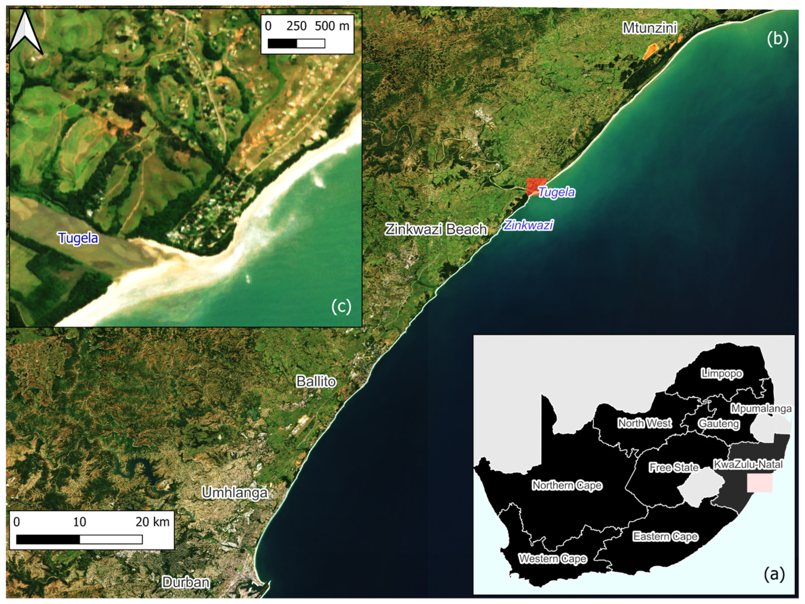
The study area spans approximately 180 km along the east coast of South Africa in KwaZulu-Natal, stretching from Durban to about 25 km south of Richards Bay (see Figure 1). Apart from Durban, one of the most populous cities in South Africa, this region includes several smaller towns, rural settlements, and estates, particularly in the southern parts, such as Umhlanga, Ballito, Zinkwazi Beach, and Mtunzini [28]. The climate is warm and temperate, with hot summers, high humidity, and total annual rainfall ranging between 1000 mm and 1200 mm [29,30].

The tidal range in Durban and Richards Bay is approximately 1.8 m, indicating a micro-tidal environment [31]. Beaches in this region are mostly dissipative or intermediate [32]. The coastline is mostly linear, predominantly featuring sandy beaches interspersed with rocky headlands [33]. Dunes are mostly parallel to the coastline, and are steep, forest-stabilised sandy formations, with most heights in the range of a few meters near the high-water mark, though they can exceed approximately 100 m inland [34,35].

The natural vegetation primarily consists of KwaZulu-Natal Coastal Belt Grassland and Northern Coastal Forest, with smaller areas of Subtropical Dune Thicket and Subtropical Seashore Vegetation [36]. The Kwazulu-Natal Coastal Belt consists of highly dissected undulating coastal plains covered by a mosaic of grasslands, coastal forests, and thickets [33]. Closer to the coast, vegetation patterns are increasingly shaped by environmental factors such as salt spray, flooding, and shifting coastal sediments [33]. These conditions drive a distinct zonation of vegetation from the shoreline inland. Ecological succession on dunes begins with pioneer plants that colonise shifting sands, forming foredunes just above the high-tide mark [34,37]. These areas transition into more stable habitats such as dune thickets or secondary scrublands, culminating in impenetrable thickets and forest [37]. Coastal dune forests typically grow on sand dunes and rolling plains, structured into distinct layers, including a tall canopy of evergreen and broadleaf trees (12–15 m), as well as a diverse understory of shrubs and ground plants (0.2–2 m) [33]. The dynamics of the estuaries present in the study area depend on their respective mouth conditions [38]. Permanently closed estuaries will be less dynamic than temporarily or permanently open estuaries, where sediment and vegetation dynamics can be either event-driven or largely marine-influenced [38]. Large estuaries feature coastal salt-marsh plains with low herbaceous vegetation dominated by succulent chenopods and other flood-tolerant halophytes, along with salt-marsh meadows of rushes and sedges, Spartina-flooded swards, and submerged Zostera sea meadows [33].

2.2. Input Data

2.2.1. Sentinel-2 Imagery

Image processing and analysis were conducted within the Google Earth Engine (GEE) cloud-based platform, which does not require local data handling or processing. Long-term Sentinel-2 imagery was used to delineate both static and dynamic boundaries of key coastal ecosystems. More specifications for the Sentinel-2 mission can be found in Drusch et al. [39]. Standardised surface-reflectance-corrected data were sourced from the Harmonized Sentinel-2 MSI: MultiSpectral Instrument, Level-2A archive, to ensure consistency across sensors and acquisition periods. The Sentinel-2 image collection was filtered to include scenes captured between 31 December 2018 and 31 December 2023 with less than 20% cloud cover and limited to tile numbers 36JUN and 36JUM. This resulted in a total of 613 images selected for classification. From these, eight images from 2022 were selected to extract spectral signatures at the training point locations to build the classification model. The eight images were selected throughout the year to account for seasonal variation in land cover, especially for vegetation classes where phenology impacts spectral reflectance values. Only a single year was used, since the primary goal was to capture representative seasonal variation rather than interannual differences, which are less pronounced for the considered land cover types. Furthermore, images from 2022 were selected to ensure temporal consistency, since the training point validation was supported through visual checks using high-resolution imagery (Google Earth) which largely corresponded to the same year.

A total of 19 bands were used as input for image classification. These included the Blue (B2), Green (B3), Red (B4), and Near-Infrared (B8) bands at 10 m resolution, as well as the Red Edge 1–3 (B5–B7), Red Edge 4 (B8A), and Shortwave Infrared 1 and 2 (B11 and B12) bands at 20 m resolution. From these original S2 bands, 9 derivative spectral images were calculated, including the Normalised Difference Vegetation Index (NDVI), Normalised Difference Built-Up Index (NDBI), Normalised Difference Water Index (NDWI), Modified NDWI (MNDWI), Enhanced Vegetation Index (EVI), Soil-Adjusted Vegetation Index (SAVI), and the three Tasselled Cap Transformation components: brightness (TCT_b), greenness (TCT_g), and wetness (TCT_w).

2.2.2. Training and Validation Data

For this research the S2 images were classified into one of four simplified land cover classes: vegetation, bare, surf, and water. These four classes were derived by merging the thirteen original land cover classes defined in the coastal land cover map by Bessinger et al. (2022) [40] into the four more general land cover types relevant to coastal dynamics. These classes were selected to ensure class representativity and model simplicity, which would highlight the key natural and geomorphological processes influencing coastal boundaries. While some parts of this coastline are densely populated, they were not assigned a distinct class. Instead, they are partially represented within bare regions, which include bare surfaces with minimal vegetation cover. Detailed urban land use assessment is beyond the scope of this study and is better addressed using national products such as the South African National Land Cover map [41].

Reference points were generated through stratified random sampling using the simplified land cover map. For each of the eight Sentinel-2 images used to extract the spectral signatures, 10 random points per class were generated for each image within the 36JUM tile, and 40 random points per class were generated for each of the images within the 36JUN tile (which spans a larger stretch of coastline). All points were sampled within a 1 km buffer of the coastline. A total of 800 reference points were collected, or 200 points per class. A summary of the collected training points can be found in Appendix A.

2.3. Image Classification

Image classification was performed in Google Earth Engine, using a Random Forest (RF) model to classify the selected 613 images. This non-parametric machine learning algorithm was selected because it presents several advantages in classification, such as efficiency in handling large datasets and robustness to overfitting, noise, and outliers [42]. It has seen widespread use for land cover and land use classification applications, and ecosystem classification [43,44,45,46]. Several studies have shown that RF models consistently yield high-accuracy results, and they are therefore well-suited for this application [42,47,48,49].

RF models are ensemble classifiers and operate through the construction of multiple DTs [50]. During the training phase, each tree is constructed using a subset of the training data (the in-bag samples), as well as a subset of the input features for classification. During the classification phase, each tree classifies each pixel in an image, and the final class is selected by calculating the mode, i.e., the output class that occurs most frequently for each pixel [50]. The implementation of the RF algorithm requires setting two user-defined parameters, including the number of trees and the number of features used in each split [50]. In this study, the number of trees was set to 500, and the number of features used in each split was set to the default number, which is the square root of the number of available features based on recommendations from earlier research [40,49,51]. The model was created using a data-splitting strategy, where 80% of the dataset was allocated for training and 20% for model validation.

2.4. Extraction of Class Appearance Frequency

Following the classification of the 613 S2 images into the four basic land cover classes, vegetation, bare, surf, and water, analysis was conducted to assess the spatial stability of each class per pixel over time. This assessment aimed to capture the dynamics of the four basic coastal land cover classes and to identify areas of stability and areas of change. For example, it was expected that the inland boundary of the coastal vegetation would remain relatively static, while the waterline, representing the boundary between beach and water, would show higher variability due to tidal states at times of fluctuations and seasonal dynamics.

To extract this information from the imagery, each image was split into four binary bands corresponding to the four land cover classes, where the presence of a class was marked as 1 and its absence as 0. This process produced four separate data cubes (or image stacks), each containing 613 binary images representing the occurrence of one land cover class per image.

In GEE, reducers summarise pixel values across image collections based on the selected functions, such as means, medians, or maxima, allowing for the efficient dimension reduction of image collections into a single image [52]. For this research, a mean reducer was then applied to each of the four stacks, which calculated the average presence of each land cover class per pixel across the time series, producing a single-band image for each class. Finally, the four single-band mean images were stacked into a single four-band image, with each band representing the average classification frequency of one land cover class. This composite image enabled a spatially explicit assessment of coastal land cover stability and changes across all classes during the selected period of analysis.

2.5. Delineation of the Static and Dynamic Coastal Zones

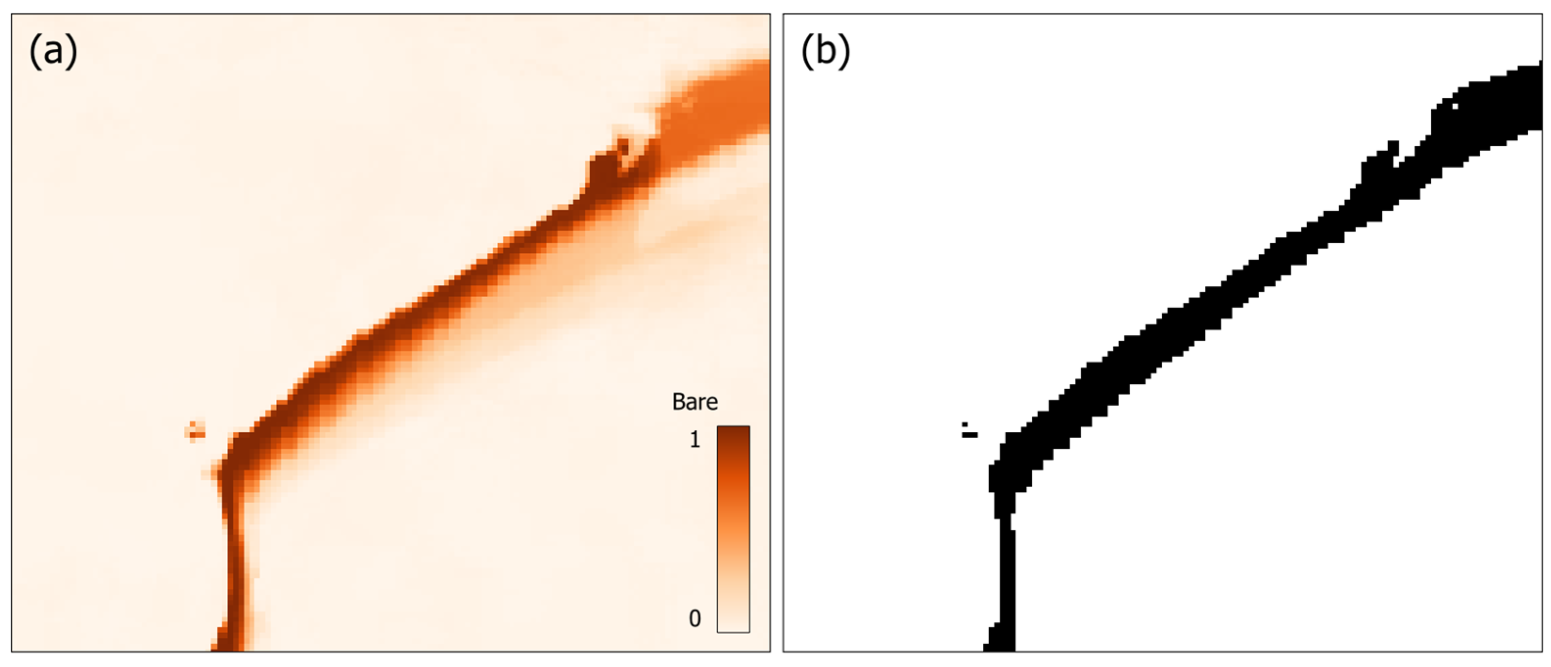
Three layers were produced for this research: a static layer depicting the stable land cover boundaries, a non-permanent vegetation zone, and the intertidal range. The static layer includes four zones: vegetation, bare, surf, and water. These areas were extracted from the class frequency bands, where the fractional value of the composite image bands for each zone exceeded 0.5. The threshold of a value greater than 0.5 for the static zones was selected because it reflects a majority class probability and provides a statistically meaningful cutoff for class membership. An illustration of the transformation from probabilistic class membership to discrete zones for the bare class is illustrated in Figure 2. The final four bands were then reclassified and merged into a single four-class image representing the static coastal zones.

The second and third layers were the two dynamic zone boundaries that were extracted: the non-permanent vegetation zone and the intertidal range, respectively. The non-permanent vegetation zone is the seashore region where pioneer plants grow since they are adapted to colonise highly dynamic beach areas, affected by occasional flooding and shifting sands [37]. Their growth facilitates the formation of hummock dunes and foredunes in areas above the spring high-tide marks [37]. The non-permanent vegetation zone was determined by extracting regions where pixel values of the vegetation bands were between 0.15 and 0.85. The intertidal range is defined as the region between the high tides and the low tides [53]. The intertidal zone was determined by merging the water and the surf bands, since both are ultimately part of the water surface, and then extracting regions where pixel values of the merged water and surf zones were between 0.15 and 0.85.

The range of 0.15 to 0.85 for the two dynamic layers was determined through trial and error to capture ecologically based transitional zones while excluding overly stable or unstable regions. For example, regions classified as water or surf more than 85% of the time could be considered permanently wet, while regions classified as such less than 15% of the time only experience infrequent events such as irregular floods. Similarly, stable vegetated areas exceed the 85% threshold, whereas frequently changing vegetated zones, such as those subject to dieback, fall below 15%. The determined thresholds delineated the regions of interest across the entire study area, showing only minor sensitivity to adjustments.

To contextualise the delineated static and dynamic coastal zones, a spatial intersection analysis was performed with the coastal subregions formally digitised by Harris et al. (2019) [14]. This allowed for quantitative comparison of class distributions within established regional typologies.

2.6. Post-Processing

Morphological filters were applied to the images to create more defined land cover class boundaries. Opening filters (erosion followed by dilation) smooth image objects and remove small details and noise, while closing filters (dilation followed by erosion) connect regions, thereby filling gaps, with both filters preserving overall object shapes and structures [54]. Opening filters were applied to the static and intertidal zone images, while a closing filter was applied to the non-permanent vegetation zone image.

A circular kernel with a one-pixel radius was applied to all filtering operations. For the static zones, the opening operation was performed by running five iterations of a focal minimum filter (erosion), followed by five iterations of a focal maximum filter (dilation), and for the intertidal zone, only one iteration for each filter was run. For the non-permanent vegetation zone, a closing operation was performed by running one iteration of a focal maximum, followed by one iteration of a focal minimum.

2.7. Accuracy Assessment

The model accuracy was determined using 20% of the reference points. Using these points, a confusion matrix was generated to compare the reference class labels with the model output classes [55]. From the confusion matrix, the Kappa statistic, user’s accuracy, and producer’s accuracy were calculated [55]. While additional metrics are occasionally employed, overall accuracy, Kappa, user’s accuracy, and producer’s accuracy remain the most common accuracy metrics in remote sensing methods [56]. Overall accuracy and the Kappa statistic provide insight into overall algorithmic performance, while user’s and producer’s accuracies are important to understand individual class performance, since high accuracies in one class may not correspond to high accuracies in another class [56].

3. Results

3.1. Model Accuracy

Table 1. Confusion matrix for the RF model. The user’s accuracy and the producer’s accuracy for each class are summarised in the last row and last column, respectively.

	Predicted Class
Reference Class	Vegetation	Bare	Surf	Water	Producer’s Accuracy
Vegetation	38	2	0	0	95
Bare	0	40	0	0	100
Surf	0	1	39	0	97.5
Water	0	0	0	40	100
User’s Accuracy	100	93.02	100	100

presents the confusion matrix which evaluates the performance of the RF model. The overall accuracy of the model was 98.13%, while the Kappa coefficient was 0.975, showing that agreement between the predicted and reference classes was high.

Performance by class also produced high results. Producer’s accuracy values for vegetation, bare, surf, and water were 95%, 100%, 97.5%, and 100%, respectively, while user’s accuracy values for vegetation, bare, surf, and water were 100%, 93.02%, 100%, and 100%, respectively. Notably, water achieved both perfect user’s and producer’s accuracies. Notable misclassifications were vegetation incorrectly classified as bare and bare areas incorrectly classified as surf.

3.2. Single-Date Classifications

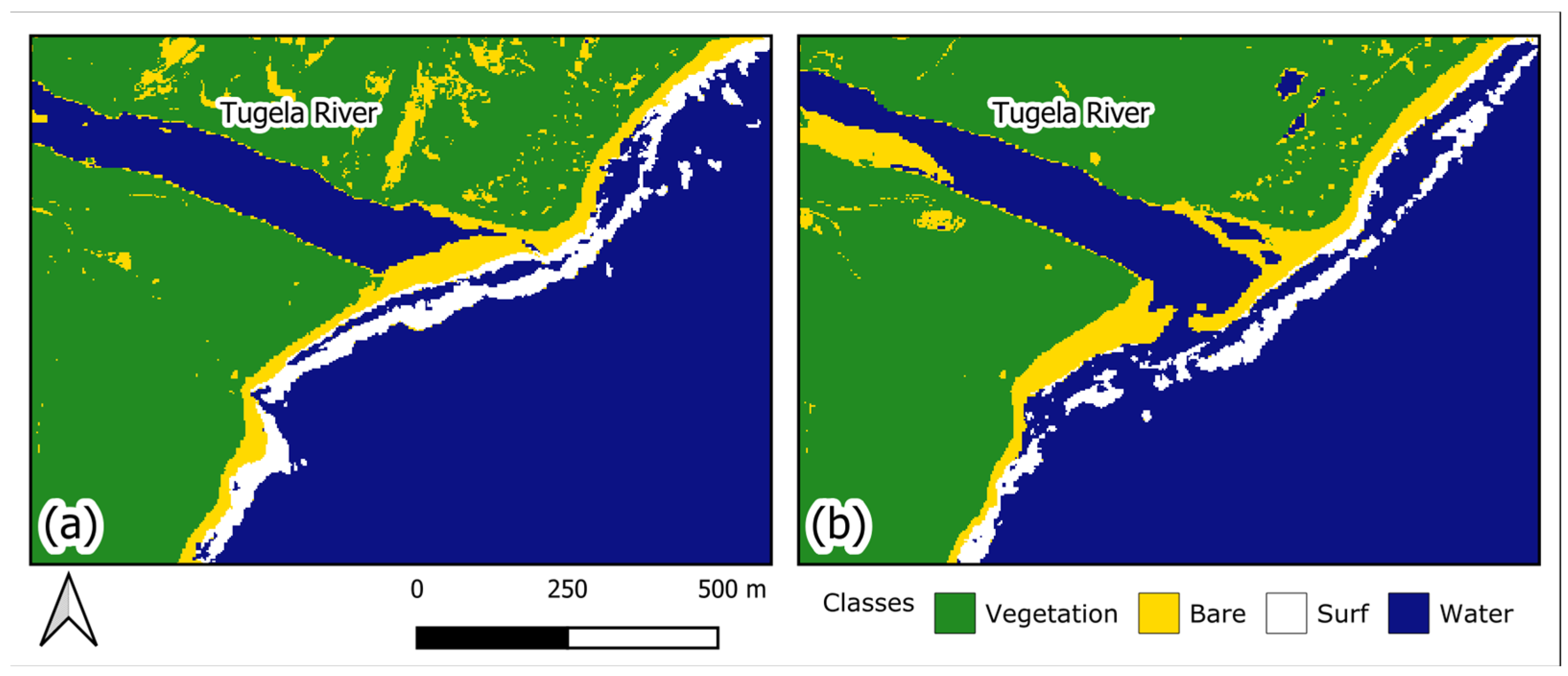
Figure 3 illustrates two single-date image classification results near the Tugela River mouth: Figure 3a shows the classification from 1 September 2019, while Figure 3b shows the classification from 6 August 2023. These two images represent noticeable differences in landscape features. In Figure 3a, the river mouth appears more closed and there is also a greater presence of bare regions along the coast. In contrast, Figure 3b shows a more open river mouth, major sediment deposition in the river, more vegetated regions along the coast, and the presence of water bodies more inland. The variations illustrate the temporal variations across time; therefore, relying on single-date imagery may not capture the overall state of the coast. Therefore, a time-series aggregation approach would provide a more reliable representation of the area’s long-term coastal dynamics.

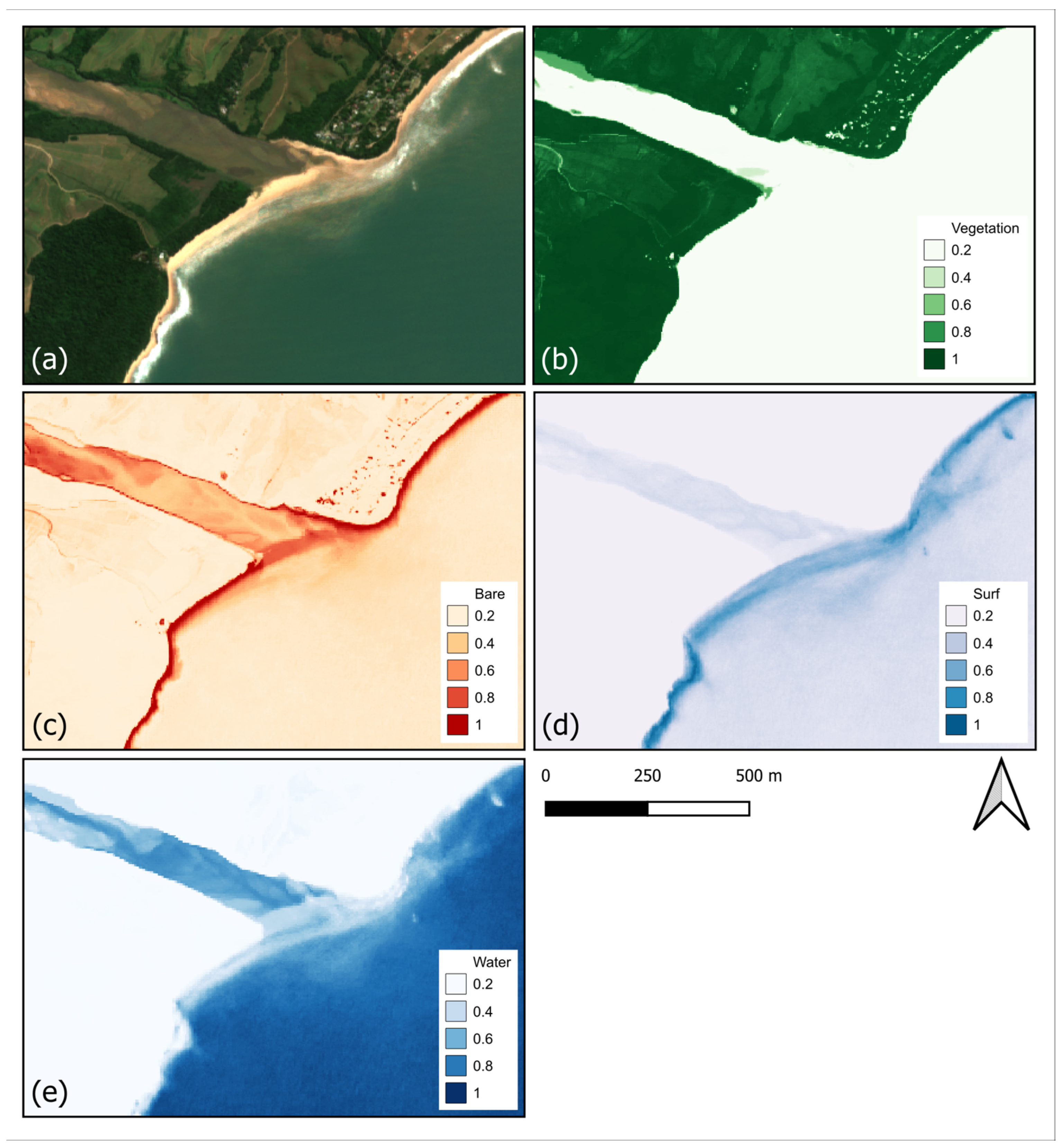
3.3. Land Cover Class Probability Bands

Figure 4 illustrates the land cover class probability bands derived from the five-year image collection in the Tugela River mouth region. Darker hues represent areas with higher classification consistency, indicating stable zones for each class, while lighter hues denote low classification frequencies, suggesting class absence or instability. Intermediate values are transitional or more dynamic areas.

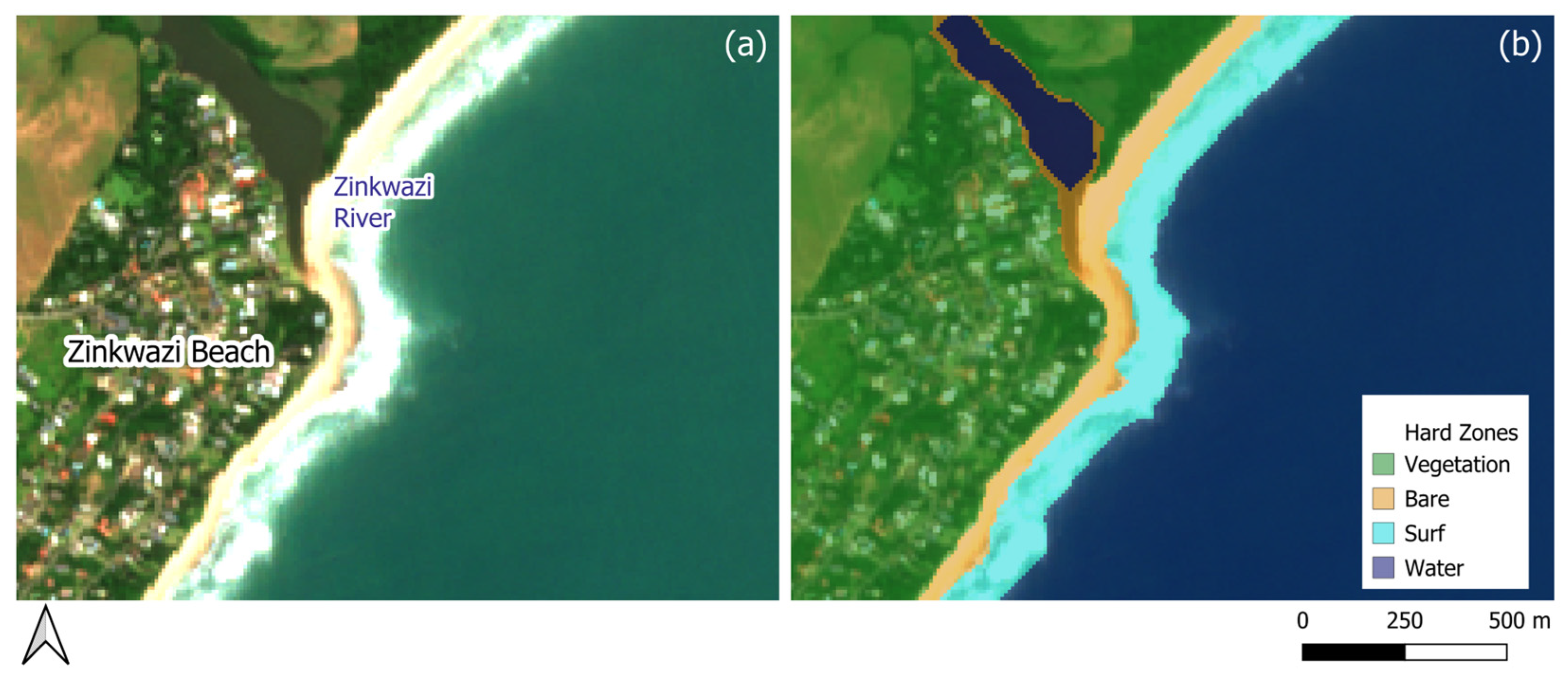
3.4. Static Zones

A more general sample of the classified static zones, where the fractional value of the raw composite image bands exceeded 0.5, can be seen in Figure 5. The resulting boundaries closely follow expected natural features. However, in the dynamic regions, classification may appear inconsistent when viewed overlayed with a single snapshot, such as bare land seeming to overlay parts of the river. This indicates where temporal aggregation differentiates persistent land cover types from the more transient ones viewed in a single snapshot.

Generally, natural area zonation is more elevation-dominated, while in urban regions, disturbances cause fragmented boundaries. In the more stable regions, where coastal forests are older and well-established, the vegetation zones appeared more well-defined and intact, and the boundaries were more linear. In contrast, in less stable zones, particularly along the foredune regions, where early successional, unstable vegetation is prevalent, significant fragmentation occurred. Similarly, more fragmented vegetation patterns were also evident in urbanised areas; vegetation patches were interspersed with built-up infrastructure. Beyond the vegetated regions, the stable bare zone generally maintained its linear appearance, closely following the beach formation and the rocky shorelines. The bare zone widened noticeably near river mouths, where high sediment deposition and dynamic fluvial processes disrupted the regular coastal profile, and fragmented along the coast. Further seaward, the surf zone exhibited a predominantly linear alignment with the coastline. However, in regions where wave dynamics led to double breaking, the surf zone fragmented, forming two distinct breaking segments.

3.5. Dynamic Zones

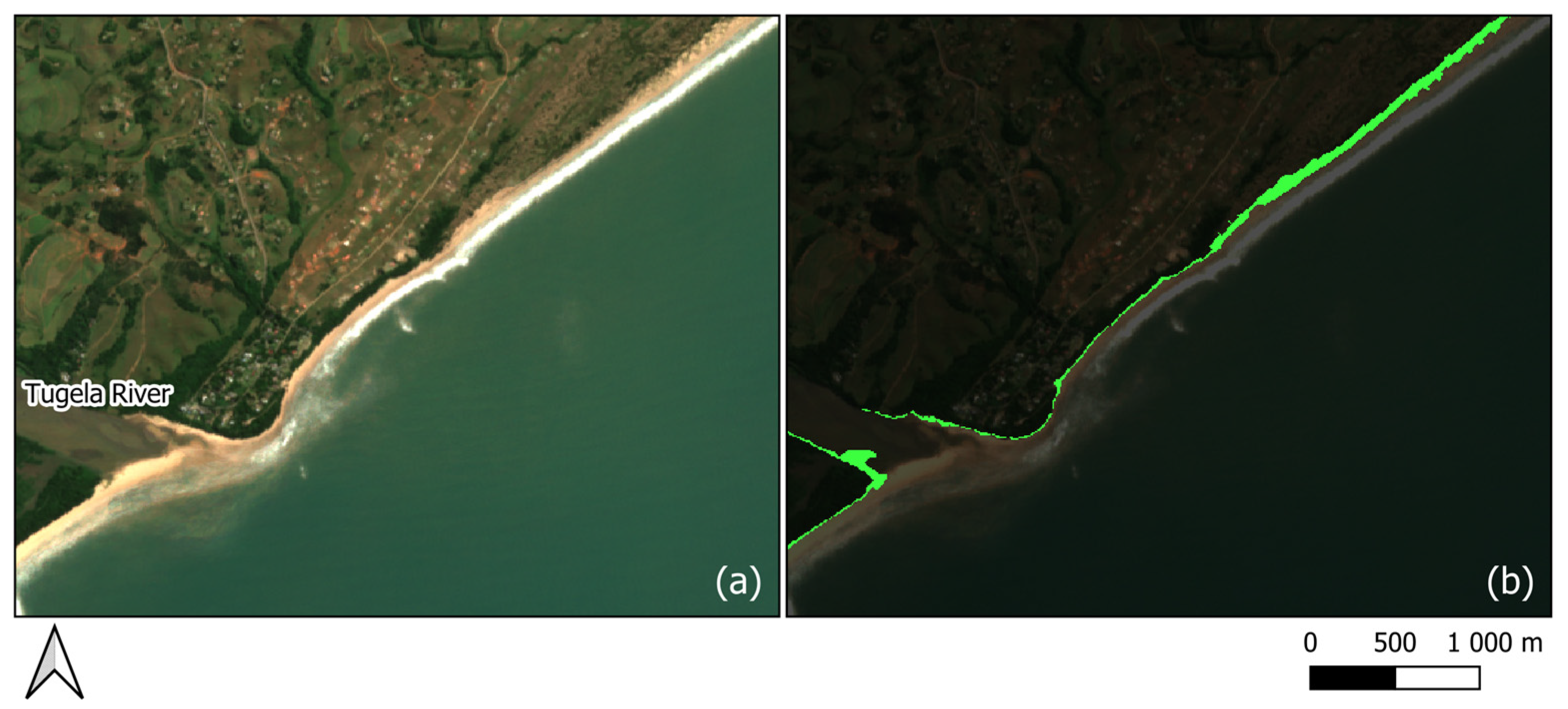
Samples of the non-permanent vegetation zones, with values ranging between 0.15 and 0.85, can be seen in Figure 6. Considerable variation can be observed within this region.

Generally, along the stabilised coastal forest regions, where dune systems are covered by mature forest vegetation, the non-permanent vegetation zone is notably narrow, which means that there is not a significant amount of variation in vegetation cover over time along these regions, and there is a sharp transition from bare regions to vegetated regions along these stretches. Conversely, the non-permanent vegetation zone widens and sometimes fragments where the unstable pioneer vegetation is prevalent on more expansive dune systems, particularly on the foredunes, where dune colonisation is more dynamic, as can be seen in the northern regions of Figure 6. Similarly, estuarine environments, characterised by more herbaceous vegetation, fewer woody species, and more frequent flooding, often exhibit broader non-permanent vegetation zones, as can be seen on the southern bank of the Tugela River in Figure 6. Additionally, in urban areas, where vegetated regions occur alongside built-up regions, the non-permanent vegetation zones appear more fragmented and extensive (Figure 7).

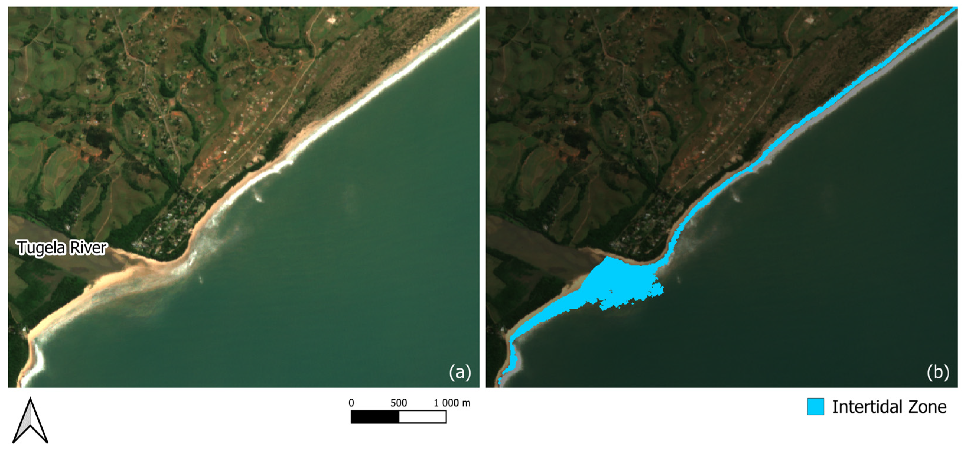
Samples of the intertidal zone, with values ranging between 0.15 and 0.85, for this stretch of coast can be seen in Figure 8. Intertidal zones exhibit notable variability across different coastal environments. On rocky outcrops as well as steeper, narrower beaches, the intertidal zones appear narrower and more fragmented, indicating a more abrupt transition between land and water. More gently sloping sandy beaches, particularly those adjacent to estuaries, display a wider intertidal zone, with fluctuating classifications between bare ground and water surfaces. In estuarine areas, the intertidal zone tends to widen due to the dynamic interaction between water and land, where sediment activity contributes to uncertainty in classifying the boundary between water and bare land (see Figure 8b near the Tugela River mouth).

3.6. Comparison with Formally Digitised Coastal Zones

Table 2. Proportional distribution of the static classes across different coastal subregions, delineated by Harris et al. (2019) [14]. Values indicate the percentage of each class found within the Coastal Marine, Coastal Vegetation, Estuarine, and Shore subregions, summing to 100% per class.

Zone	Coastal Marine	Coastal Vegetation	Estuarine	Shore	Total
Bare	0.28%	18.88%	41.55%	39.29%	100%
Surf	0.65%	1.79%	0.19%	97.37%	100%
Vegetation	0.00%	86.37%	13.38%	0.25%	100%
Water	64.64%	0.06%	12.31%	22.98%	100%

presents the distribution of the static zones across all coastal subregions. Values are presented as percentages, which indicate the relative intersections of each class within the respective subregions.

The vegetation zone primarily overlapped with the Coastal Vegetation subregion (86.37%), followed by the Estuarine zone (13.38%), and minimal overlap occurred in the Shore subregion (0.25%). Bare zones primarily overlapped with Estuarine (41.55%) and Shore (39.29%) subregions, with a minor but notable presence within the Coastal Vegetation subregion (18.88%). Surf almost exclusively overlapped with the Shore subregion (97.37%), with negligible representation in other zones. Water was mainly distributed across the Coastal Marine subregion (64.64%), with some overlap in the Shore (22.98%) and Estuarine (12.31%) subregions.

In contrast to the static zones, intersections observed between the more dynamic zones and the existing coastal classification differ notably.

Table 3. Proportional distribution of the dynamic classes across different coastal subregions, delineated by Harris et al. (2019) [14]. Values indicate the percentage of each class found within the Coastal Marine, Coastal Vegetation, Estuarine, and Shore subregions, summing to 100% per class.

Zone	Coastal Marine	Coastal Vegetation	Estuarine	Shore	Total
Intertidal zone	0.97%	6.59%	40.75%	51.69%	100.00%
Non-permanent vegetation zone	0.00%	65.96%	27.50%	6.54%	100.00%

presents the distribution of the intertidal zone and the non-permanent vegetation zone across all coastal subregions. Values are presented as percentages, which indicate the relative intersections of each class within the respective subregions.

The intertidal zone predominantly intersects the Shore (51.69%) and Estuarine (40.75%) subregions. There is minimal intersection with the Coastal Vegetation subregion (6.59%), while intersection with the Coastal Marine subregions is minimal (0.97%). Conversely, the non-permanent vegetation zone primarily intersects with the Coastal Vegetation subregion (65.96%), followed by the Estuarine subregion (27.5%). There is minimal intersection within the Shore region (6.54%) and no intersection within the Coastal Marine subregion.

4. Discussion

4.1. Classification Accuracy

The high accuracy results highlight the reliability of the model and its robustness in delineating the four selected land cover types, even with a limited set of training points. The consistently high producer’s and user’s accuracies confirm the model’s ability to reliably distinguish between the four classes. Vegetation was, however, sometimes misclassified as bare areas, which suggests some confusion between these two classes in certain instances, likely in the transition zones, where pixels are more mixed. This is primarily due to vegetation in these regions being sparse, patchy, or low-lying, often intermixed with bright sandy beaches whose reflectance signal can dominate the spectral signature, leading to misclassification. Despite this, the overall performance highlights the appropriate selection of the land cover types. The high accuracies, aided by the basic categorisation and more separable spectral signatures, therefore demonstrate the suitability of the method for capturing both static and dynamic coastal zonation patterns across a time-series dataset.

4.2. Static Coastal Zones

The static zones indicate the more stable regions of the coast and reflect persistent, long-term ecological and anthropogenic processes. In the more stable regions, the continuity and linearity of coastal vegetation suggest well-developed ecological succession and dune stabilisation, with minimal disturbance. The presence of mature forests is characterised by dense vegetation and narrow pioneer zones, indicating low levels of mobility [57]. In contrast, fragmented vegetation patterns, particularly near urban regions or foredunes, either reflect the dynamic conditions (such as sand movement, wind, and pioneer plant communities) or anthropogenic interference which disrupts successional trajectories and connectivity. These spatial patterns illustrate how natural and human activities shape coastal vegetation, with implications for habitat connectivity and the resilience of coastal ecosystems [9].

The static bare and surf zones further illustrate underlying coastal processes. Their linear appearance, especially in stable dune systems, suggests consistent sediment flux, stable depositional patterns, and sustained wave energy in the sandy regions [58]. The widening near the river mouths reflects fluvial systems such as freshwater outflows, sediment transport, and variations in seasonal discharge. Moreover, fragmented or double-breaking surf zones indicate the presence of submerged sandbars or underwater topographic shifts which alter wave dynamics and therefore surf zone boundaries [58]. Overall, the spatial patterns within the static zone reflect class stability and maturity, as well as physical processes shaping the coast.

Furthermore, their distribution within the existing classification of the coastline aligns with expected ecological characteristics. For instance, the static vegetation zone mostly intersects the Inland Coastal and vegetated Estuarine subregions. Similarly, bare regions primarily intersect Shore and unvegetated sections of Estuarine subregions, which aligns with known constraints on plant growth in sparsely vegetated regions, such as flooding, sediment movement, unstable soils, and high salinity [9,59]. The surf zone intersects mainly with the Shore subregion, consistent with its definition as the seaward extent of the shoreline [14]. The water zone primarily intersects with the Coastal Marine subregion, as expected, but extends to the Shore and Estuarine subregions, reflecting the transitional nature towards the seaward shoreline as well as the significant hydrological components of estuarine environments.

4.3. Dynamic Coastal Zones

In contrast to static regions, the dynamic regions highlight regions of higher environmental variability and disturbance. The broader, patchier appearance of non-permanent vegetation zones in the foredune regions and estuarine regions indicates high mobility, early successional communities, and stressors such as inundation or salt exposure [34]. In contrast, narrow, clearly defined transition zones suggest stabilised systems where vegetation has reached an equilibrium with sand or water movement [33,34]. Furthermore, transitional areas adjacent to urban zones exhibit highly fragmented patterns, highlighting how anthropogenic pressures disrupt the successional stages of vegetation and make the transition between vegetation and bare regions less predictable [60].

Similarly, the intertidal zone varies in width and continuity, based on factors such as slope, sediment supply, tides, and currents. Steeper, narrower beaches; rocky areas; and riverbanks exhibit narrower, more fragmented intertidal zones and compress the vertical tidal range, reducing the horizontal displacement, resulting in a narrower intertidal area. In contrast, gently sloping sandy beaches and estuarine environments tend to have wider intertidal zones, due to gradual gradients, more uniform wave and tidal action, and sediment transport. In estuaries, this widening is further driven by the interaction of tidal forces, freshwater inflow, and high sediment supply, which leads to the formation of mudflats and marshes through ongoing deposition and erosion, leading to less distinct boundaries between land and water. However, the width of these zones fluctuates in response to seasonal discharge, wave activity, and the periodic opening and closure of the river mouth [61,62].

The distribution of dynamic zones within existing coastal classifications suggests that the determination of dynamic zones can enhance the representation of these shifting regions within static classifications. For example, the intertidal zone primarily intersects the Shore (51.69%) and Estuarine (40.75%) subregions, both of which represent transitional environments. This reinforces the idea that intertidal areas are transitional between marine and the terrestrial ecosystems. Limited overlap with the Coastal Marine (0.97%) and Coastal Vegetation (6.59%) subregions is also consistent with their more clearly defined ecosystem types: either predominantly water or coastal vegetation located above the intertidal zone. In contrast, non-permanent vegetation overwhelmingly intersected the Coastal Vegetation subregion (65.96%), which highlights its presence in dune systems and ephemeral vegetation. The secondary overlap with the Estuarine subregion (27.5%) further underscores the transitional nature of estuarine habitats, where vegetation is regularly inundated due to tidal influence.

4.4. Implications of Mapping Static and Dynamic Coastal Regions

The identification of static and dynamic regions along the coast provides a useful tool to monitor landscape variations and changes. Static regions represent areas of long-term stability or limited disturbance, often due to protection or natural resilience, and highlight regions of low variability. In contrast, dynamic regions experience frequent shifts driven by coastal processes such as erosion, deposition, and vegetation turnover [63,64]. This distinction is useful for planning and risk management, since dynamic areas could potentially act as early indicators of environmental response to stressors such as storms, sea-level rise, or coastal development [65]. This could potentially inform resilience planning, guide restoration priority areas, and support hazard mitigation strategies.

In terms of conservation, the identification of dynamic habitats supports climate change adaptation strategies by identifying the areas which are most subject to change or ecosystem threats. This supports adaptive conservation prioritisation, enabling early intervention in vulnerable zones. The distinction between static and dynamic coastal zones therefore supports integrated coastal management by informing anticipatory and resilient governance.

4.5. Comparison with Existing Boundary Delineation Methods

Traditional research that captures transitional coastal boundaries has often employed simple thresholding or fuzzy logic or probabilistic models to determine class membership [23,66,67]. While these studies achieved high classification performance (e.g., over 90% agreement or mean deviations of less than 12 m from the coastline), the resulting outputs were still discrete boundaries. More recent studies which used multitemporal data to extract dynamic intertidal zones reported strong agreement with elevation data (R² values up to 0.95) [68,69]. This study builds on these methods by extending the approach beyond the intertidal zone to include dynamic vegetation zones, successfully extracting ecologically significant regions based on class persistence and variability over time, demonstrating high classification accuracy using a confusion matrix-based assessment.

5. Limitations and Future Research

Despite high model accuracy and robust delineations, some limitations with this approach to coastal delineation persist. A key limitation is the spatial resolution, where medium-resolution satellites such as Landsat and Sentinel-2 are used to delineate very narrow coastal boundaries, such as pioneer zones and wetland regions [70,71]. Shoreline displacement errors with such imagery typically range between 3 and 11 m [71]. This method is therefore unsuitable for cadastral applications or site-specific engineering. However, while higher-resolution imagery provides finer detail, the limited coverage and higher cost make them less suitable for frequent, large-scale monitoring. Medium-resolution data, with more frequent revisit times, are therefore more practical for trend analysis. These data are therefore useful for regional-scale assessments by mapping broader functional zones that offer spatial and temporal context for coastal planning and management. In dynamic coastal landscapes, where fixed boundaries often conflict with naturally shifting features, this zonation method enables a more realistic interpretation of change over time.

Furthermore, misclassifications are common in complex, dynamic environments and transitional zones such as coastal areas, where mixed pixels often result in incorrect classification of water, bare ground, and vegetation [72]. Inspection of the fractional band showed that such misclassifications can propagate through time-series data, which introduces uncertainty in delineating the extent of coastal features, especially in more dynamic regions.

Despite limitations, the RF model consistently identified coastal zones with a high degree of accuracy over the five-year time frame. The strong alignment between qualitative observations and quantitative assessments supports the effectiveness of using S2 time-series data to extract both static and dynamic coastal classes through a probabilistic class-membership approach. Future research should expand on this approach by monitoring coastal zonation shifts over time, thereby enabling the detection of directional trends, as well as linking drivers that shape coastal geomorphology to these directional trends.

6. Conclusions

This research used hyper-temporal image cubes to delineate the static and the dynamic coastal boundaries along a portion of the coast of KwaZulu-Natal. The use of a long-term image stack allows for the extraction of persistent features, which not only reduces noise, but also ensures a reduction in the temporal anomalies which can potentially be encountered in single-date imagery. The data align well with established coastal classifications while also showing spatial discrepancies which suggest regions that potentially need refinement.

The static zones, which were identified by their more persistent probabilistic class membership over time, were shown to be useful for the delineation of stable coastal zones. In contrast, the dynamic zones captured areas of greater variation, thereby identifying regions more susceptible to change due to various coastal processes such as tides, sedimentation, vegetation turnover, and anthropogenic disturbance. These outputs support enhanced delineation of coastal zones and can inform spatial planning, conservation, and risk management. The identification of stable regions using the approach in this research can provide reliable baselines for coastal planning and management, while mapping more dynamic areas helps highlight where adaptive policies are needed due to greater uncertainty.

A key limitation of this approach lies in the spatial resolution of Sentinel-2 imagery, which is suitable for large-scale monitoring but may not accurately reflect fine-scale features such as narrow, sub-pixel dune vegetation bands or cadastral boundaries. Thus, these data are better suited for regional assessments, long-term trend detection, and identifying areas of coastal change or instability. Furthermore, they can support policy and management decisions that require information about the variability and ecological significance of transitional boundaries, such as the HWM, which is often used in legal and planning frameworks but is inherently uncertain due to natural variability and measurement challenges. The use of the non-permanent vegetation zone and the intertidal zone to recontextualise boundaries within a probabilistic framework enhances the understanding of coastlines as transitional zones, subject to dynamic shoreline movement, and not simply discrete boundaries. This can inform more adaptive, resilience-based governance strategies.

The results therefore indicate that, despite the limitations highlighted, Sentinel-2 imagery can be used to delineate the coastal environment effectively. Tools which support more rapid and adaptive responses to dynamic coastal environments are essential. Long-term imagery, combined with cloud-computing technologies, offers a cost-effective and scalable solution for regular coastal zone and boundary delineation, thereby enhancing adaptation efforts and supporting effective coastal management.