


Localization of Multiple GNSS Interference Sources Based on Target Detection in C/N0 Distribution Maps

Abstract
1. Introduction
1.1. Related Work
1.2. Our Contribution
2. Materials and Methods
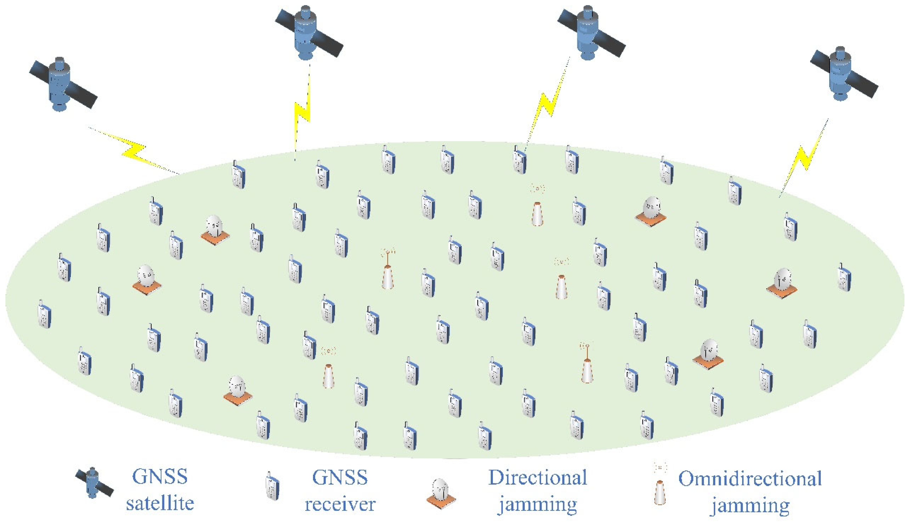
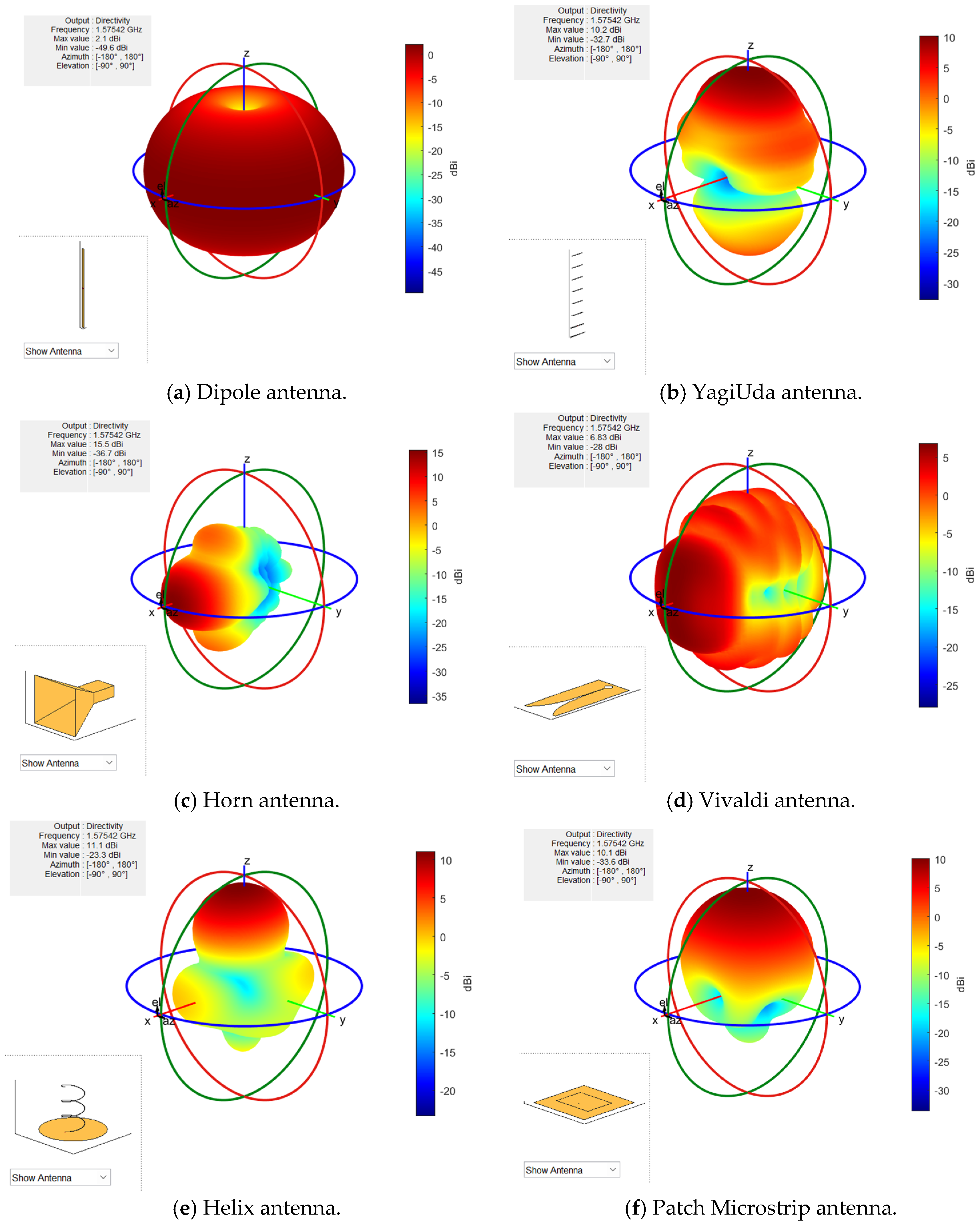
2.1. System Model
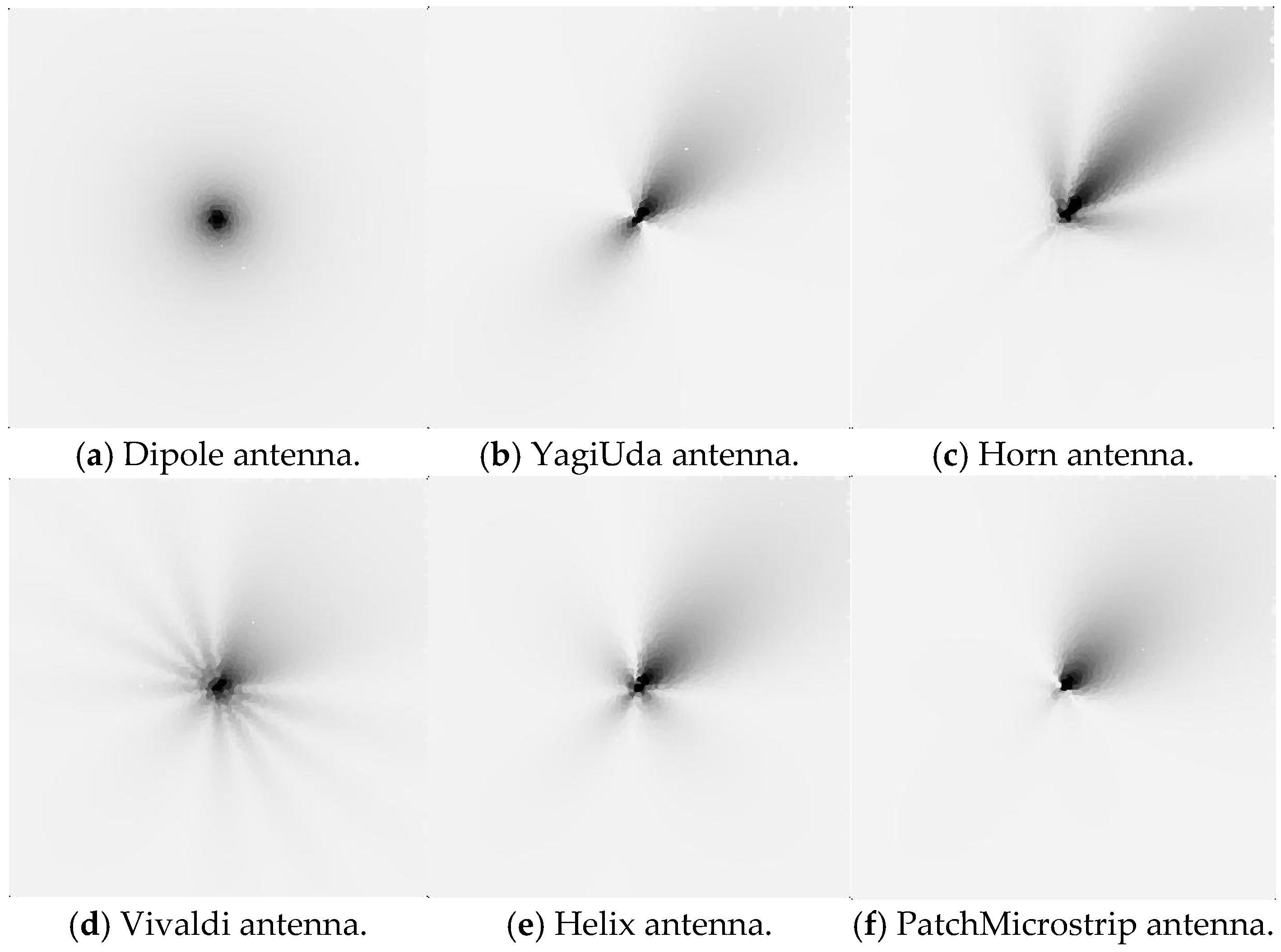
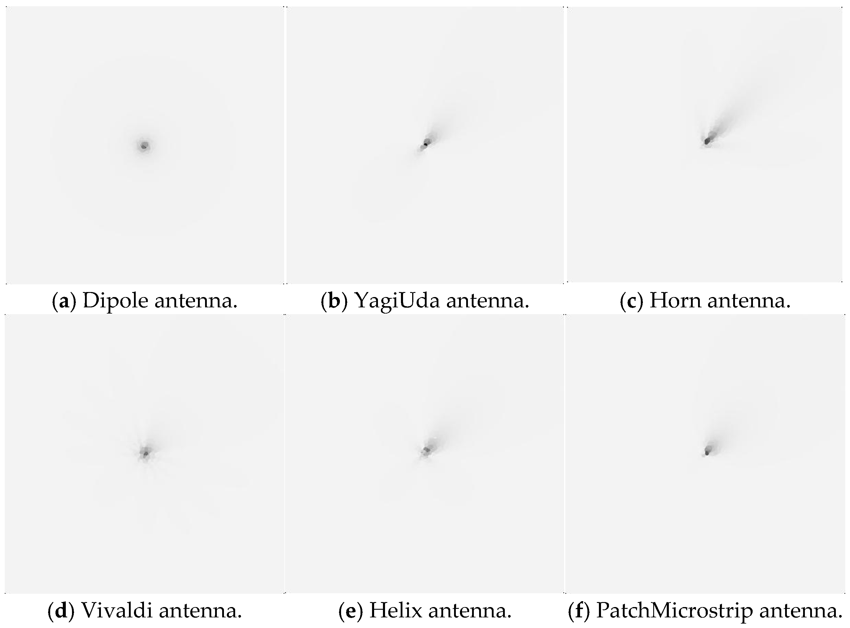
2.2. C/N0 Distribution Map Construction Method
| Algorithm 1: Generation method of the CNR distribution map |
| INPUT: The number of receivers M |
| INPUT: Monitoring area width length L and width W |
| INPUT: The receiver returned data set |
| INPUT: The C/N0 threshold |
| INPUT: The C/N0 value under interference-free |
| INPUT: Set the distance threshold for selecting C/N0 data when assigning grayscale values to pixels |
| OUTPUT: The C/N0 distribution map ICN |
| 1: Calculate receiver density as |
| 2: Set the localization accuracy as |
| 3: Calculate the width of the C/N0 distribution map as , the height of the C/N0 distribution map as , and the number of pixels as |
| 4: Initialize the gray values of all pixels in the C/N0 distribution map ICN to 0 corresponding to the C/N0 under interference-free conditions |
| 5: While do |
| 6: Obtain the receiver returned data set that are within a distance of from the pixel |
| 7: Calculate the weighted average of the C/N0 data for the DM data points, where the weights are the inverse of the distance to the pixel |
| 8: If then |
| 9: Calculate the grayscale value corresponding to the value using Formula (8) and write it to the corresponding pixel |
| 10: Else |
| 11: Write the grayscale value 255 to the corresponding pixel |
| 12: End if |
| 13: End while |
| 14: Perform a dilation operation on ICN |
| 15: Perform a median filtering operation on ICN |
| 16: Return the C/N0 distribution map ICN |
2.3. Dataset Generation and Problem Description
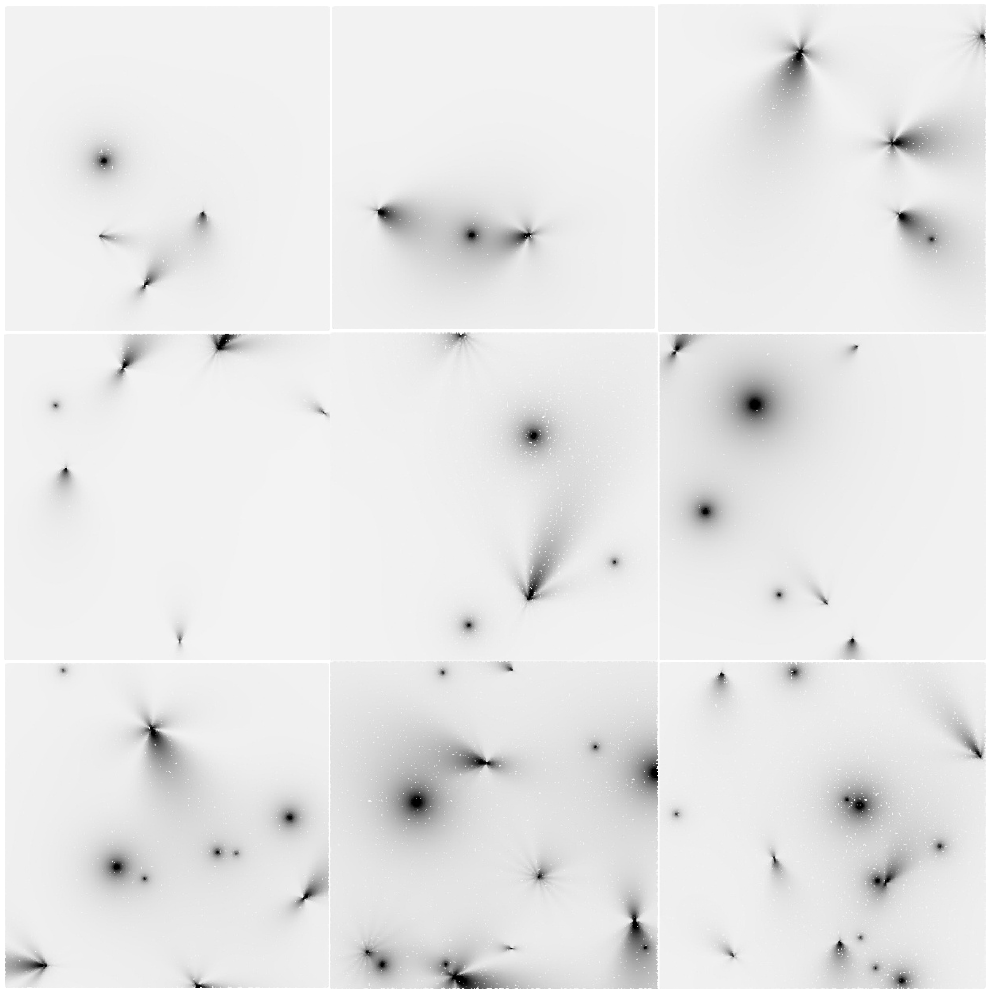
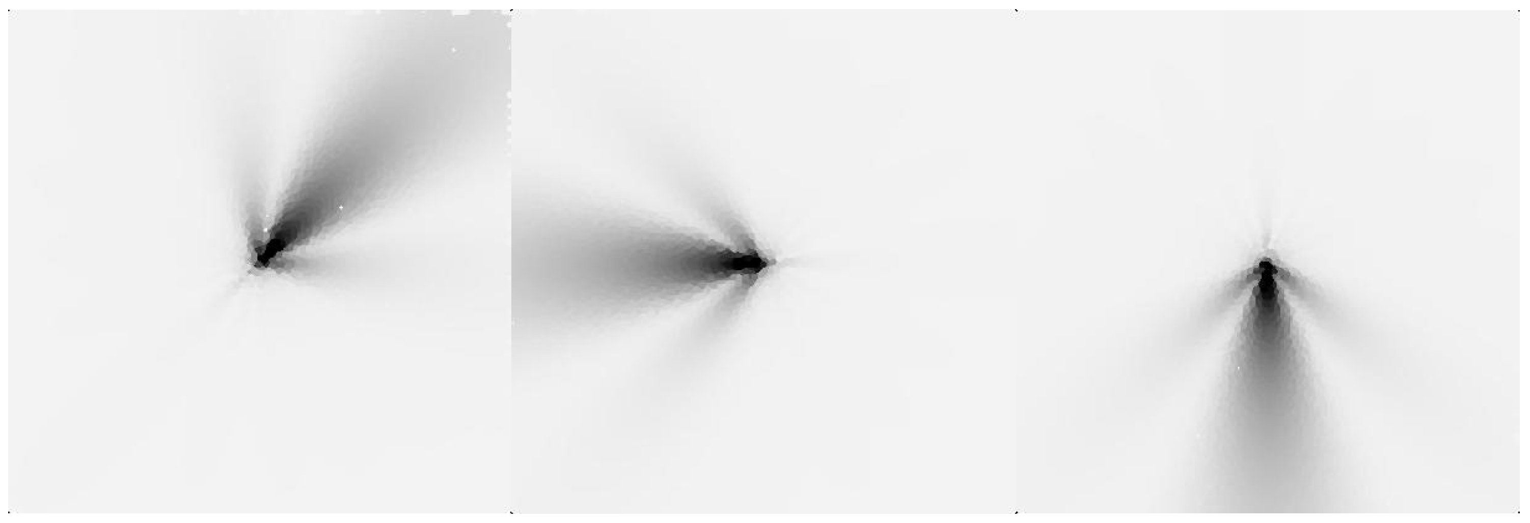
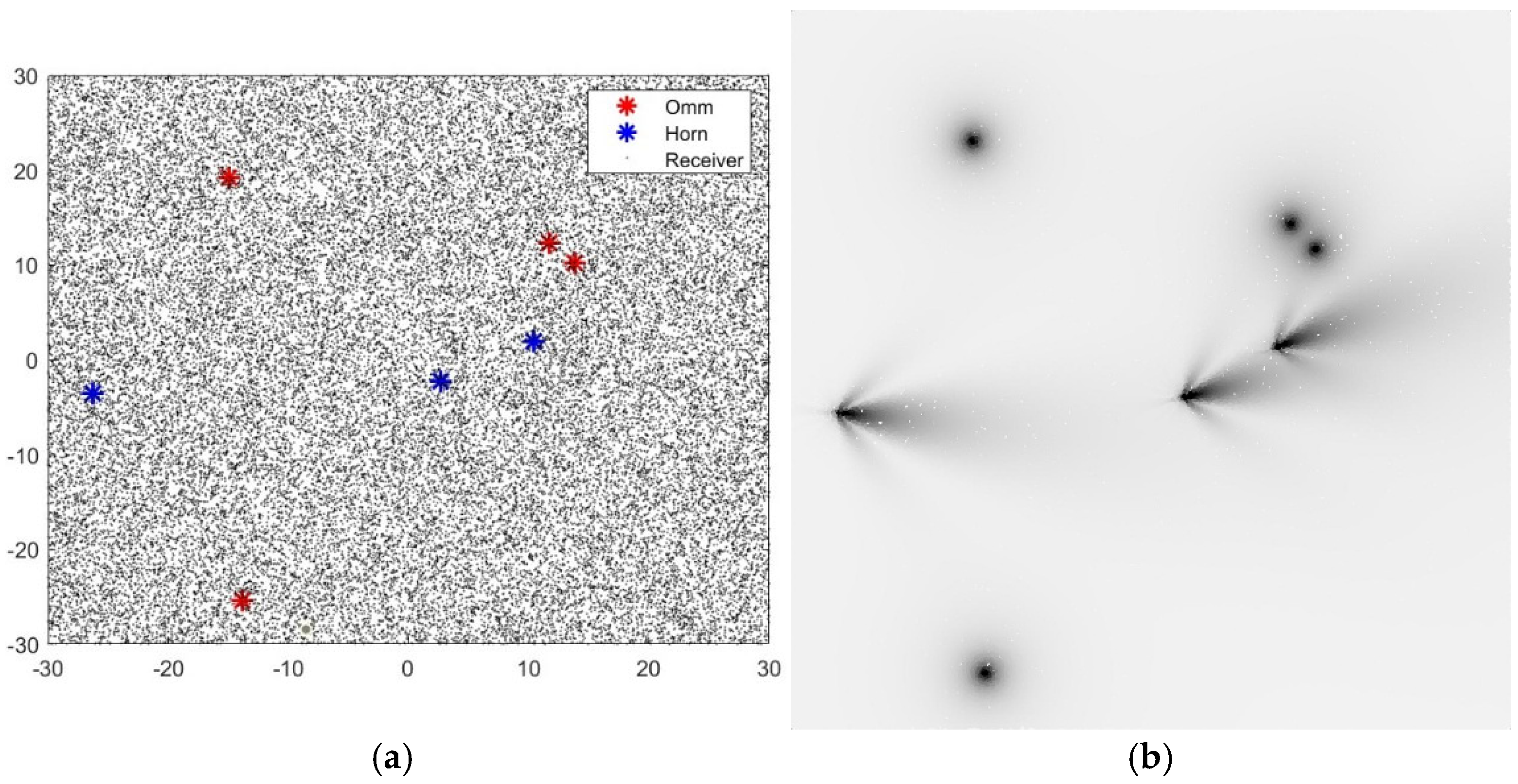
2.3.1. Dataset Generation
2.3.2. Problem Description
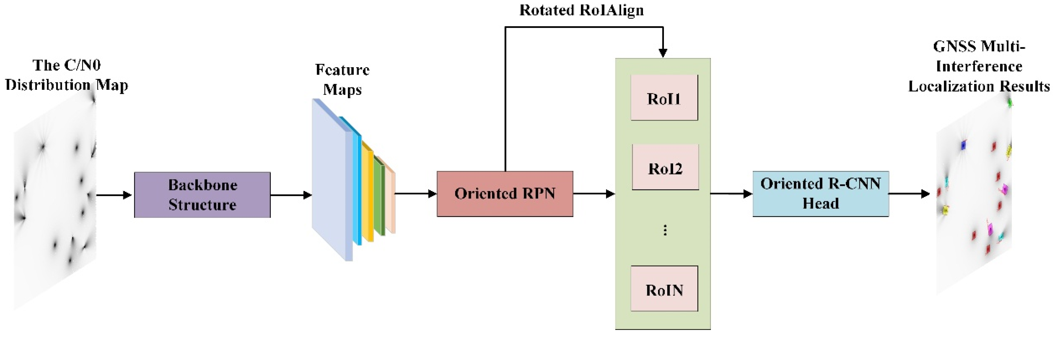
2.4. OSF-RCNN
2.4.1. Algorithmic Framework
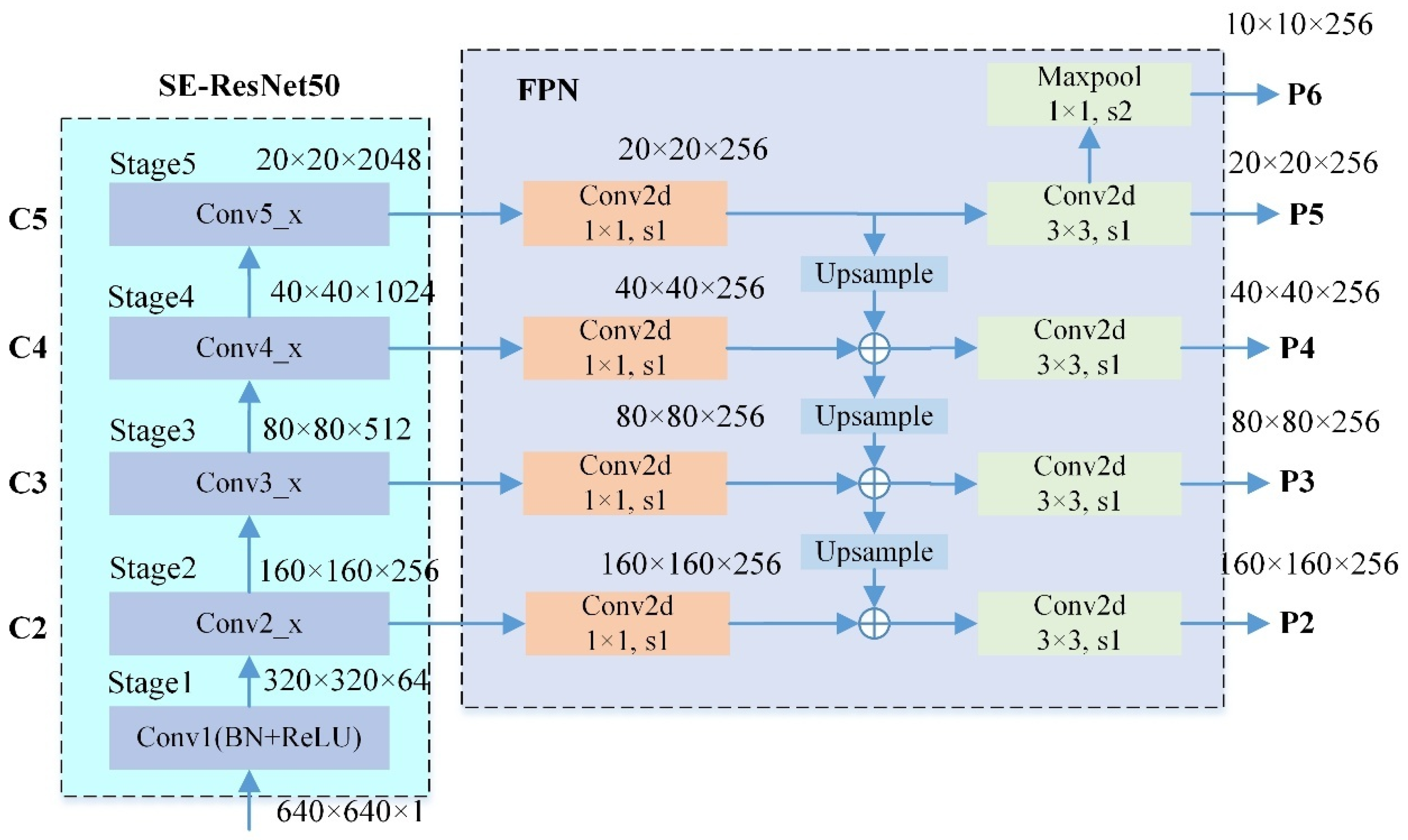
2.4.2. Backbone Structure
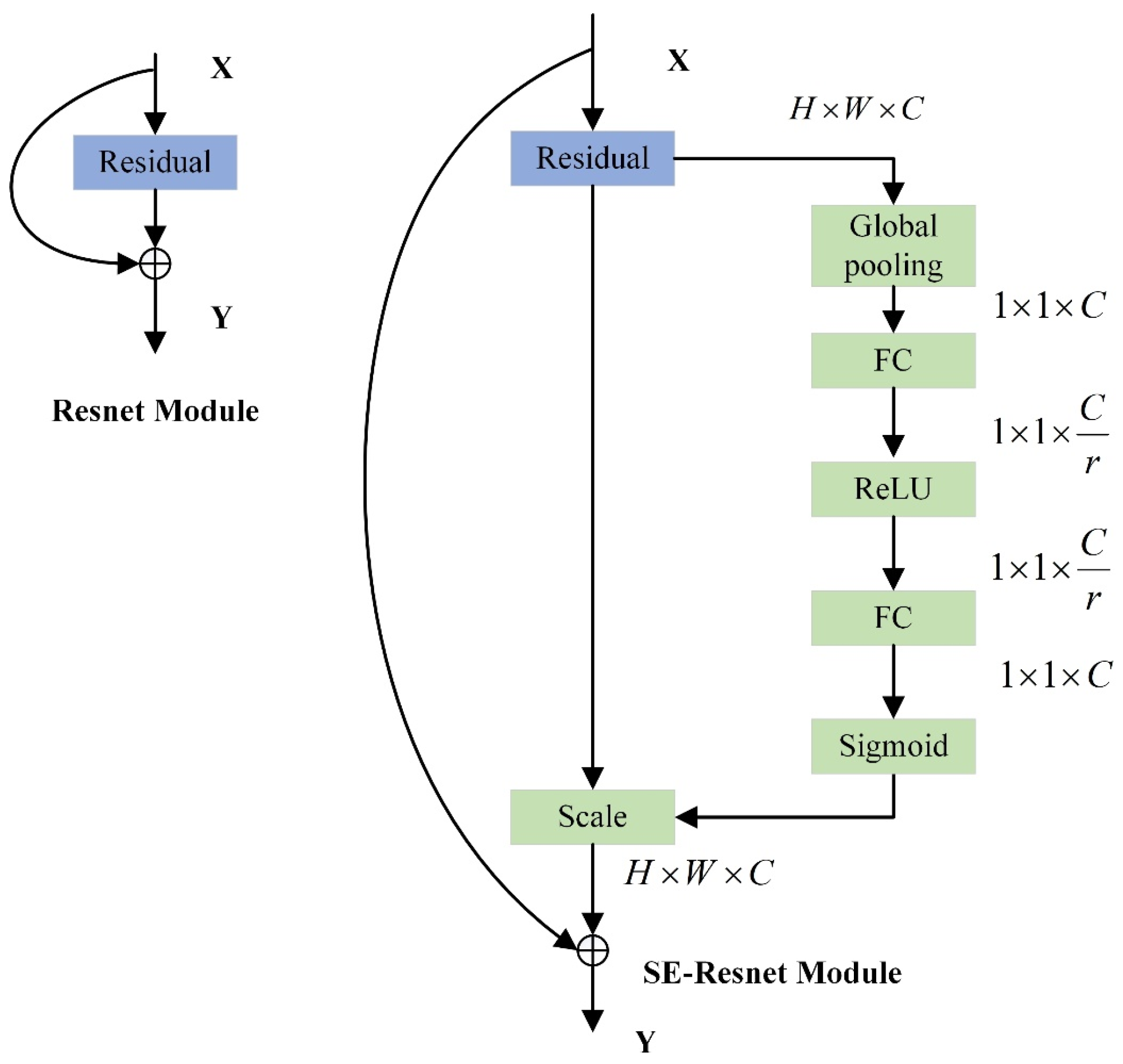
2.4.3. SE Mechanism
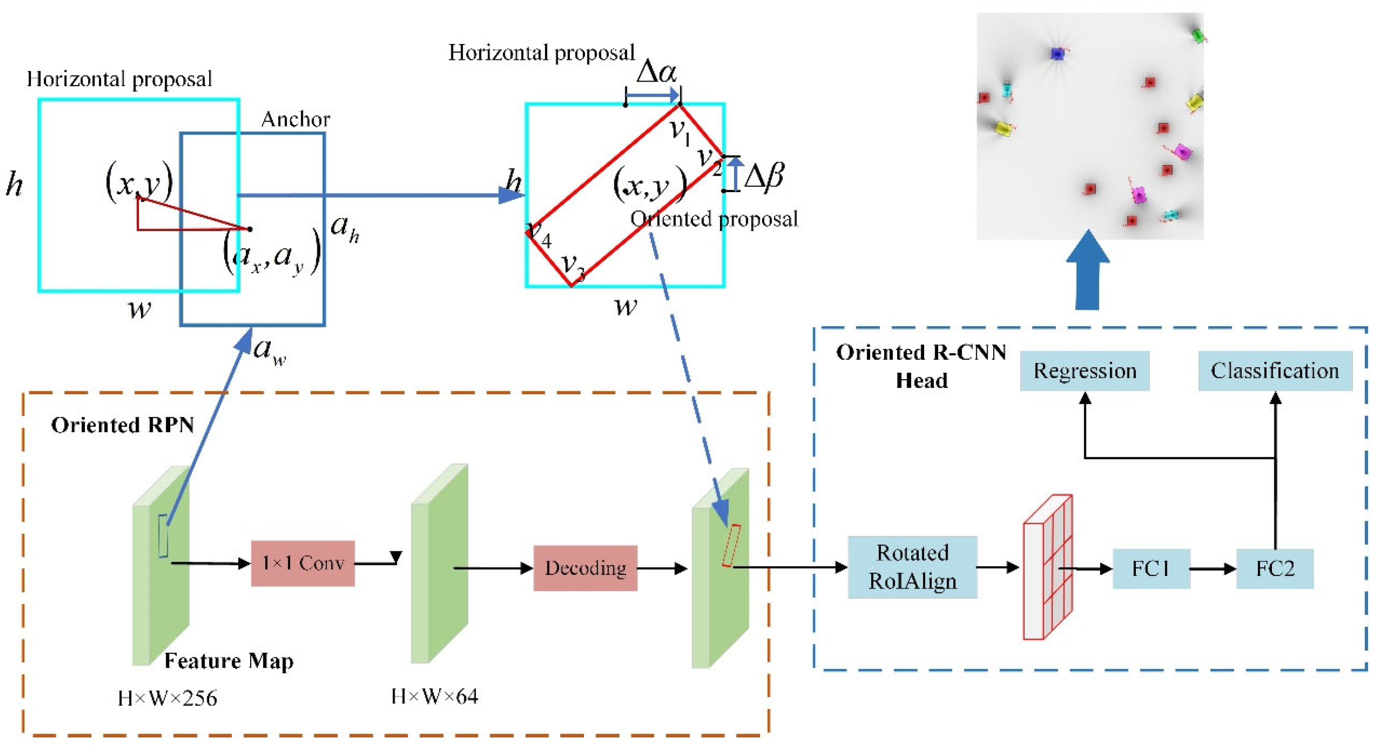
2.4.4. Oriented RPN
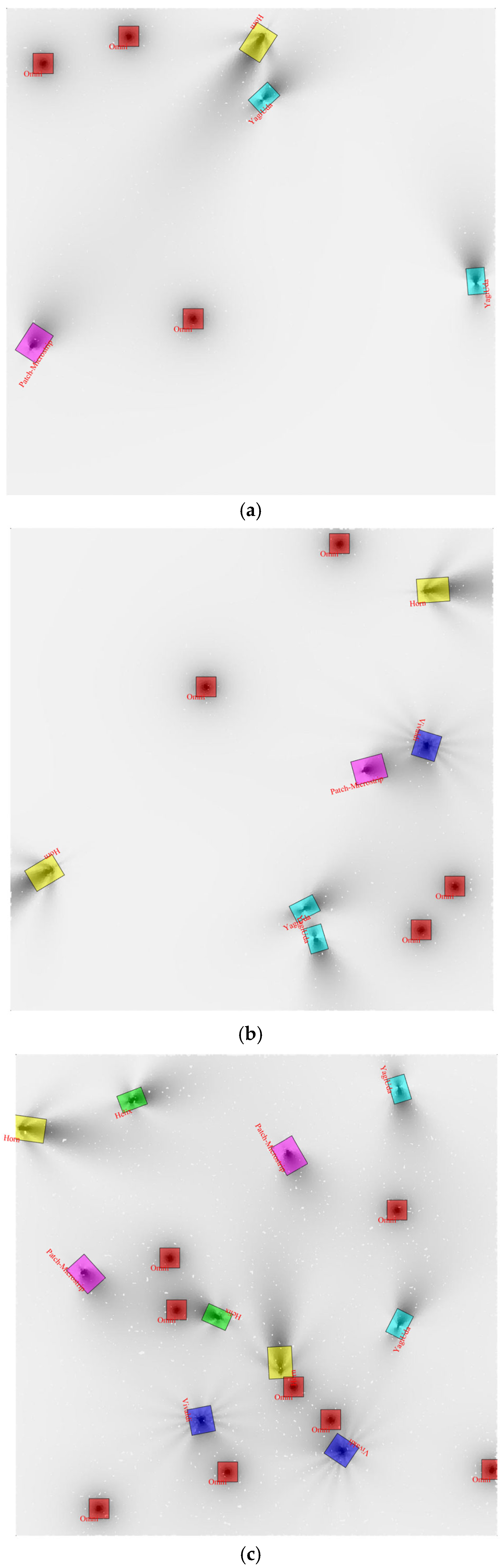
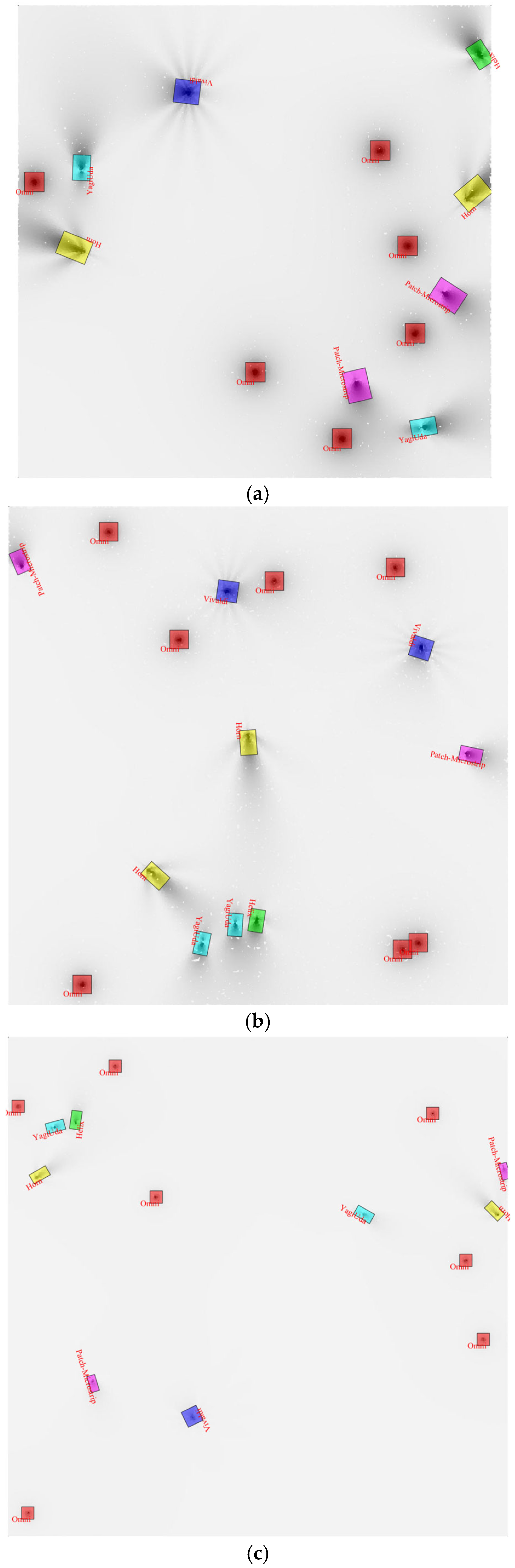
3. Results and Discussion
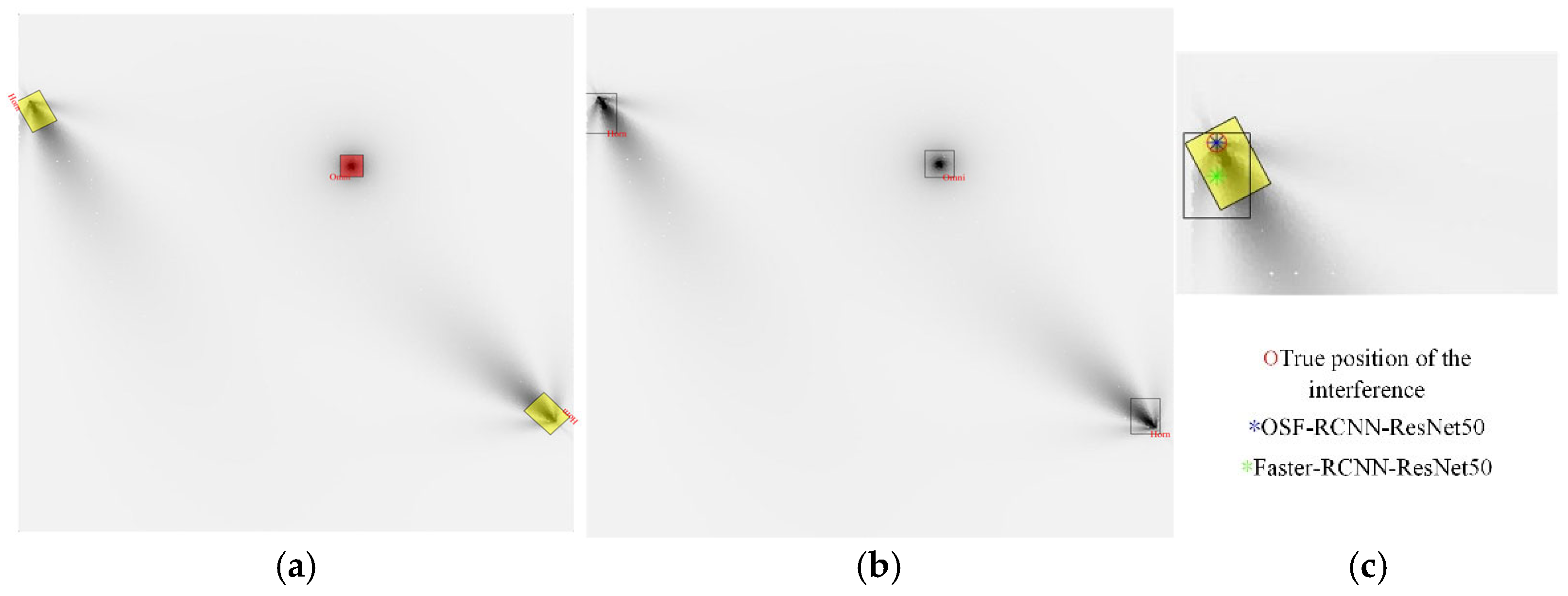
3.1. Experiment 1: Simulation of Detection and Localization Performance for Directional Interference Sources
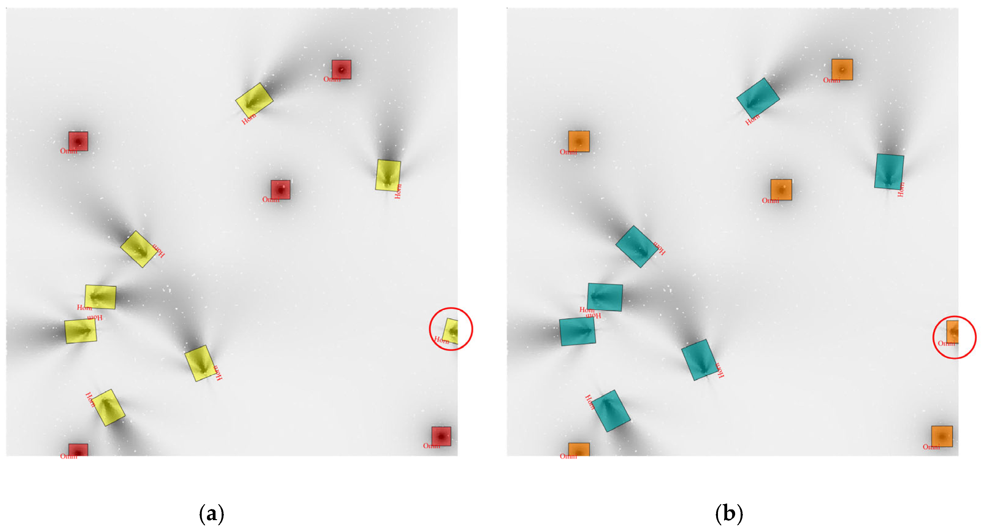
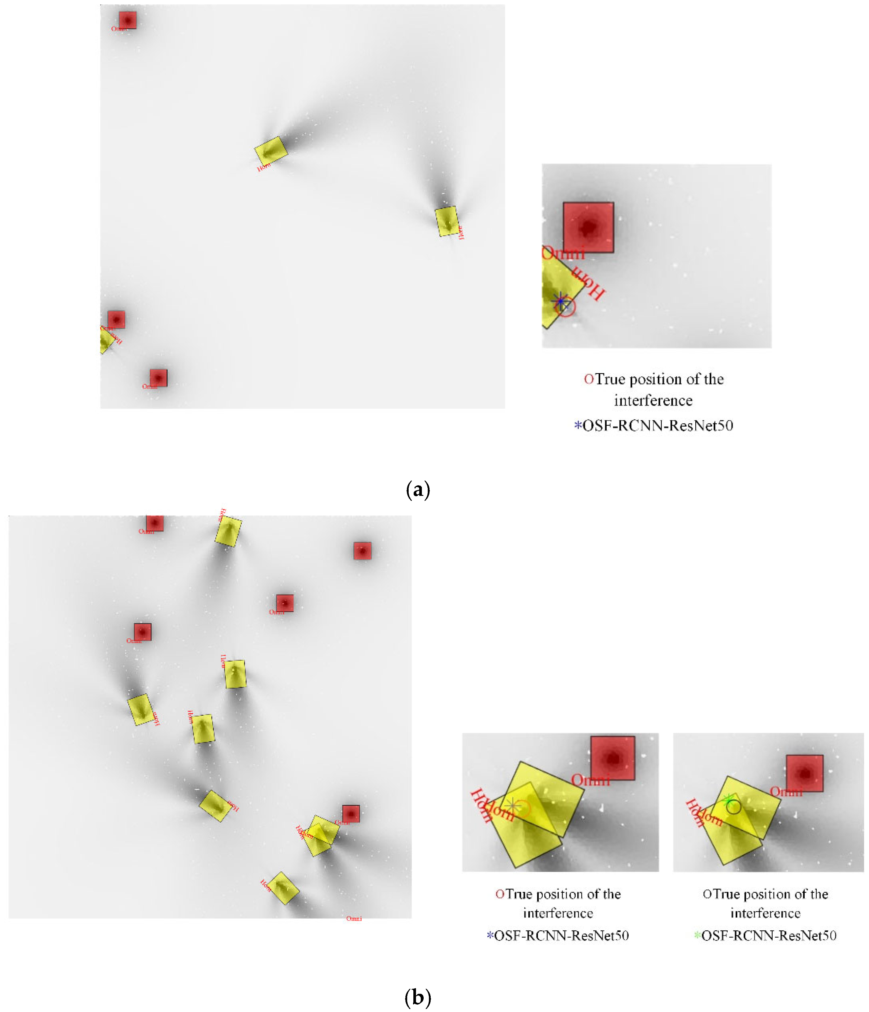
3.2. Experiment 2: Simulation of Detection and Localization Performance for Multi-Type Interference Sources
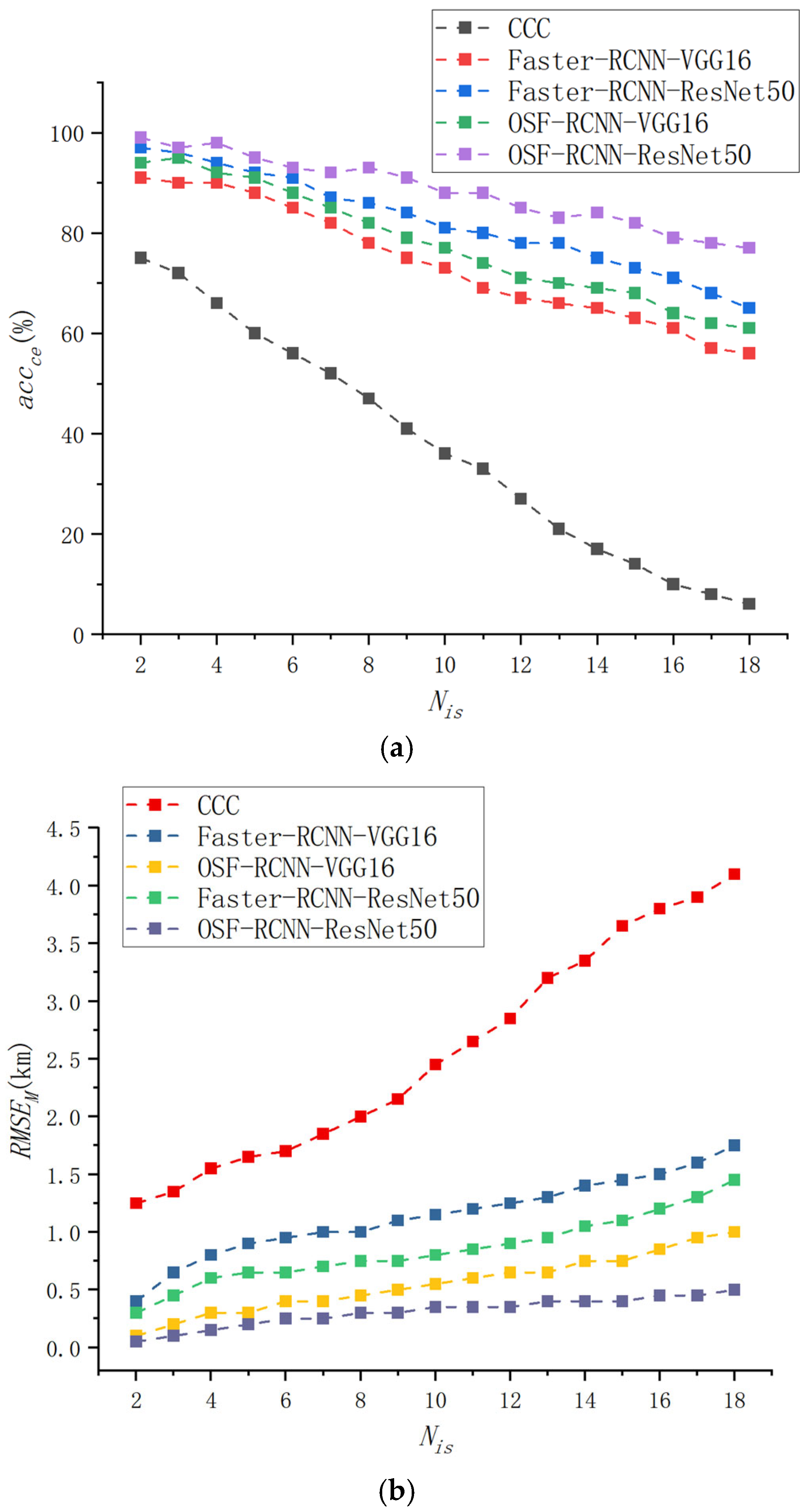
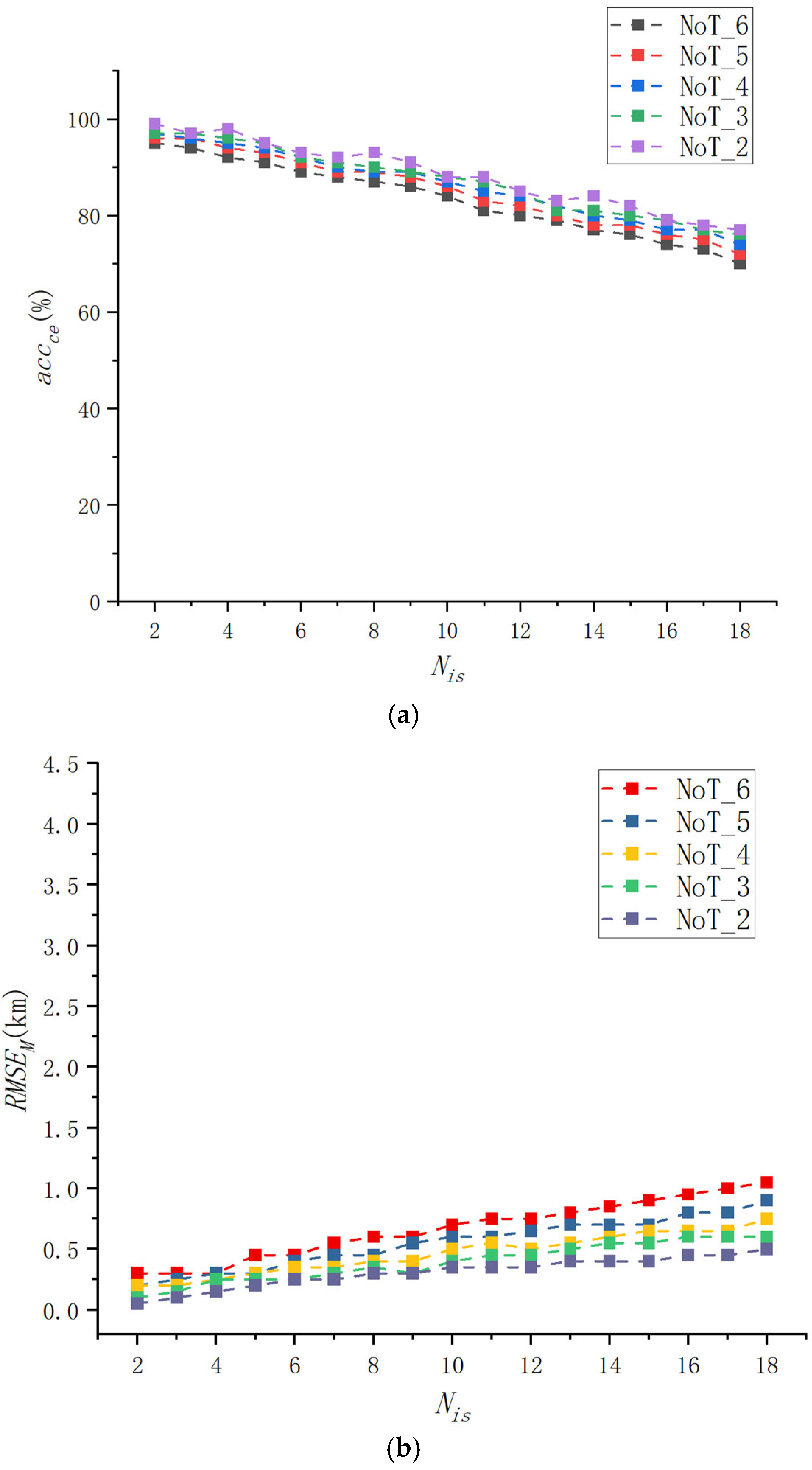
3.3. Experiment 3: Simulation of Detection and Localization Performance Under Varying Interference Transmission Powers
4. Conclusions
Author Contributions
Funding
Data Availability Statement
Conflicts of Interest
Abbreviations
| GNSS | Global Navigation Satellite Systems |
| C/N0 | Carrier-to-noise ratio |
| OSF-RCNN | Oriented Squeeze-and-Excitation-based Faster Region-based Convolutional Neural Network |
| Faster R-CNN | Faster Region-based Convolutional Neural Network |
| RPN | Region Proposal Network |
| SE | Squeeze-and-Excitation |
| FPN | Feature Pyramid Network |
| GPS | Global Positioning System |
| GLONASS | Global Navigation Satellite System |
| DOA | Direction of Arrival |
| TDOA | Time Difference of Arrival |
| RSS | Received Signal Strength |
| COTS | Commercial off-the-shelf |
| MIIT | Ministry of Industry and Information Technology |
| J911 | Jamming 911 |
| ION | Institute of Navigation |
| SVM | Support Vector Machine |
| RCNN | Region-based Convolutional Neural Network |
| YOLO | You Only Look Once |
| ResNet | Residual Network |
| RoIs | Regions of Interest |
| FC | Fully connected |
| RoIAlign | Rotated Region of Interest Align |
| SE-ResNet50 | SE-enhanced ResNet50 |
| MLP | Multilayer perceptron |
| IoU | Intersection over Union |
| VGG | Visual Geometry Group |
| RMSE | Root Mean Square Error |
References
- Kaplan, E.D.; Hegarty, C. (Eds.) Understanding GPS: Principles and Applications, 2nd ed.; Artech House Publishers: Norwood, MA, USA, 2005. [Google Scholar]
- Borre, K.; Akos, D.; Bertelsen, N.; Rinder, P.; Jensen, S. A Software–Defined GPS and Galileo Receive: Single–Frequency Approach; Birkhäuser: Boston, MA, USA, 2007. [Google Scholar]
- Dardari, D.; Closas, P.; Djurić, P.M. Indoor tracking: Theory, methods, and technologies. IEEE Trans. Veh. Technol. 2015, 64, 1263–1278. [Google Scholar] [CrossRef]
- Wu, R.; Wang, W.; Lu, D.; Wang, L.; Jia, Q. Adaptive interference mitigation in GNSS; Springer: Singapore, 2018. [Google Scholar]
- Wang, H.; Yao, Z.; Yang, J.; Fan, Z. A Novel Beamforming Algorithm for GNSS Receivers with Dual-Polarized Sensitive Arrays in the Joint Space–Time-Polarization Domain. Sensors 2018, 18, 4506. [Google Scholar] [CrossRef] [PubMed]
- Balaei, A.T.; Motella, B.; Dempster, A.G. GPS interference detected in Sydney-Australia. In Proceedings of the IGNSS Conference, Sydney, Australia, 4–6 December 2007; pp. 1–12. [Google Scholar]
- Kuusniemi, H.; Airos, E.; Bhuiyan, M.Z.H.; Kröger, T. GNSS jammers: How vulnerable are consumer grade satellite navigation receivers. Eur. J. Navig. 2012, 10, 14–21. [Google Scholar]
- Dempster, A.G.; Cetin, E. Interference Localization for Satellite Navigation Systems. Proc. IEEE 2016, 104, 1318–1326. [Google Scholar] [CrossRef]
- Bhamidipati, S.; Gao, G.X. GPS Multireceiver Joint Direct Time Estimation and Spoofer Localization. IEEE Trans. Aerosp. Electron. Syst. 2018, 55, 1907–1919. [Google Scholar] [CrossRef]
- Gao, G.X.; Sgammini, M.; Lu, M.; Kubo, N. Protecting GNSS Receivers from Jamming and Interference. Proc. IEEE 2016, 104, 1327–1338. [Google Scholar] [CrossRef]
- Rounds, S. Innovation-Jamming Protection of GPS Receivers-Part II: Antenna Enhancements-The second article in a two-part series about jamming protection for GPS receivers looks at enhancements to antenna. GPS World 2004, 15, 38–45. [Google Scholar]
- Daneshmand, S.; Jafarnia-Jahromi, A.; Broumandan, A.; Lachapelle, G. A GNSS structural interference mitigation technique using antenna array processing. In Proceedings of the 2014 IEEE 8th Sensor Array and Multichannel Signal Processing Workshop, A Coruna, Spain, 22–25 June 2014. [Google Scholar]
- Zhang, J.; Cui, X.; Xu, H.; Lu, M. A Two-Stage Interference Suppression Scheme Based on Antenna Array for GNSS Jamming and Spoofing. Sensors 2019, 19, 3870. [Google Scholar] [CrossRef] [PubMed]
- Amin, M.G.; Wang, X.; Zhang, Y.D.; Ahmad, F.; Aboutanios, E. Sparse Arrays and Sampling for Interference Mitigation and DOA Estimation in GNSS. Proc. IEEE 2016, 104, 1302–1317. [Google Scholar] [CrossRef]
- Fresno, J.M.; Robles, G.; Martínez-Tarifa, J.M.; Stewart, B.G. Survey on the Performance of Source Localization Algorithms. Sensors 2017, 17, 2666. [Google Scholar] [CrossRef] [PubMed]
- Amin, M.G.; Borio, D.; Zhang, Y.D.; Galleani, L. Time-Frequency Analysis for GNSSs: From interference mitigation to system monitoring. IEEE Signal Process. Mag. 2017, 34, 85–95. [Google Scholar] [CrossRef]
- Borio, D.; Gioia, C.; Štern, A.; Dimc, F.; Baldini, G. Jammer Localization: From Crowdsourcing to Synthetic Detection. In Proceedings of the 29th International Technical Meeting of The Satellite Division of the Institute of Navigation, Manassas, VA, USA, 12–16 September 2016; pp. 3107–3116. [Google Scholar] [CrossRef]
- Wang, P.; Morton, Y.T. Efficient Weighted Centroid Technique for Crowdsourcing GNSS RFI Localization Using Differential RSS. IEEE Trans. Aerosp. Electron. Syst. 2020, 56, 2471–2477. [Google Scholar] [CrossRef]
- Mills, K.; Ahmad, F.; Amin, M.G.; Himed, B. Fast Iterative Interpolated Beamforming for Interference DOA Estimation in GNSS Receivers Using Fully Augmentable Arrays. In Proceedings of the 2019 IEEE Radar Conference (RadarConf), Toulon, France, 23–27 September 2019; pp. 1–5. [Google Scholar] [CrossRef]
- Chen, Q.D.; Tao, H.H.; Liu, R.; Zhen, W.M. Time Difference Estimation Method for TDOA Location of GNSS Weak Interference. J. China Acad. Electron. Inf. Technol. 2020, 15, 135–140. (In Chinese) [Google Scholar] [CrossRef]
- Khandker, S.; Torres-Sospedra, J.; Ristaniemi, T. Analysis of Received Signal Strength Quantization in Fingerprinting Localization. Sensors 2020, 20, 3203. [Google Scholar] [CrossRef] [PubMed]
- Statistical Bulletin of the Communications Industry of the Central People’s Government of the People’s Republic of China in 2023. Available online: https://www.gov.cn/lianbo/bumen/202401/content_6928019.htm (accessed on 1 June 2025).
- Strizic, L.; Akos, D.M.; Lo, S. Crowdsourcing GNSS Jammer Detection and Localization. In Proceedings of the 2018 International Technical Meeting of The Institute of Navigation, Reston, VA, USA, 29 January–1 February 2018; pp. 626–641. [Google Scholar]
- Scott, L. J911: The case for fast jammer detection and location using crowdsourcing approaches. In Proceedings of the 24th International Technical Meeting of The Satellite Division of the Institute of Navigation (ION GNSS 2011), Portland, OR, USA, 19–23 September 2011; pp. 1931–1940. [Google Scholar]
- Liu, R.; Yang, Z.; Chen, Q.; Liao, G.; Zhen, W. GNSS multi-interference source centroid location based on clustering centroid convergence. IEEE Access 2021, 9, 108452–108465. [Google Scholar] [CrossRef]
- Shafi, M.; Takada, J. Advances in Propagation Modeling for Wireless Systems. In EURASIP Journal on Wireless Communications and Networking; Hindawi Publishing Corporation: London, UK, 2009; p. 5. [Google Scholar]
- Burger, W.; Burge, M.J. Digital Image Processing: An Algorithmic Introduction; Springer Nature: London, UK, 2022. [Google Scholar]
- Eddins, S.L.; Gonzalez, R.C.; Woods, R.E. Digital Image Processing Using Matlab; Princeton Hall Pearson Education Inc.: Hoboken, NJ, USA, 2004; pp. 6–12. [Google Scholar]
- Xie, G. Principles of GPS and Receiver Design; Publishing House of Electronics Industry: Beijing, China, 2009; pp. 244–246. [Google Scholar]
- Zou, Z.; Chen, K.; Shi, Z.; Guo, Y.; Ye, J. Object detection in 20 years: A survey. Proc. IEEE 2023, 111, 257–276. [Google Scholar] [CrossRef]
- Mittal, P.; Singh, R.; Sharma, A. Deep learning-based object detection in low-altitude UAV datasets: A survey. Image Vis. Comput. 2020, 104, 104046. [Google Scholar] [CrossRef]
- Chen, C.; Zheng, Z.; Xu, T.; Guo, S.; Feng, S.; Yao, W.; Lan, Y. YOLO-Based UAV Technology: A Review of the Research and Its Applications. Drones 2023, 7, 190. [Google Scholar] [CrossRef]
- Yan, D.; Li, G.; Li, X.; Zhang, H.; Lei, H.; Lu, K.; Chen, M.; Zhu, F. An improved faster R-CNN method to detect tailings ponds from high-resolution remote sensing images. Remote Sens. 2021, 13, 2052. [Google Scholar] [CrossRef]
- Xie, X.; Cheng, G.; Wang, J.; Yao, X.; Han, J. Oriented R-CNN for object detection. In Proceedings of the IEEE/CVF International Conference on Computer Vision, Montreal, QC, Canada, 10–17 October 2021; pp. 3520–3529. [Google Scholar]
- Hu, J.; Shen, L.; Sun, G. Squeeze-and-excitation networks. In Proceedings of the IEEE Conference on Computer Vision and Pattern Recognition, Salt Lake City, UT, USA, 18–23 June 2018; pp. 7132–7141. [Google Scholar]
- Lin, T.Y.; Dollár, P.; Girshick, R.; He, K.; Hariharan, B.; Belongie, S. Feature pyramid networks for object detection. In Proceedings of the IEEE Conference on Computer Vision and Pattern Recognition, Honolulu, HI, USA, 21–26 July 2017; pp. 2117–2125. [Google Scholar]
- Kirillov, A.; He, K.; Girshick, R.; Dollár, P. A unified architecture for instance and semantic segmentation. In Proceedings of the IEEE Conference on Computer Vision and Pattern Recognition, Honolulu, HI, USA, 21–26 July 2017. [Google Scholar]
- Cai, Z.; Vasconcelos, N. Cascade r-cnn: Delving into high quality object detection. In Proceedings of the IEEE Conference on Computer Vision and Pattern Recognition, Salt Lake City, UT, USA, 18–23 June 2018; pp. 6154–6162. [Google Scholar]
- Wu, F.; Lin, H. Effect of transfer learning on the performance of VGGNet-16 and ResNet-50 for the classification of organic and residual waste. Front. Environ. Sci. 2022, 10, 1043843. [Google Scholar] [CrossRef]

Disclaimer/Publisher’s Note: The statements, opinions and data contained in all publications are solely those of the individual author(s) and contributor(s) and not of MDPI and/or the editor(s). MDPI and/or the editor(s) disclaim responsibility for any injury to people or property resulting from any ideas, methods, instructions or products referred to in the content. |
© 2025 by the authors. Licensee MDPI, Basel, Switzerland. This article is an open access article distributed under the terms and conditions of the Creative Commons Attribution (CC BY) license (https://creativecommons.org/licenses/by/4.0/).
Share and Cite
Chen, Q.; Liu, R.; Yan, Q.; Xu, Y.; Liu, Y.; Huang, X.; Zhang, Y. Localization of Multiple GNSS Interference Sources Based on Target Detection in C/N0 Distribution Maps. Remote Sens. 2025, 17, 2627. https://doi.org/10.3390/rs17152627
Chen Q, Liu R, Yan Q, Xu Y, Liu Y, Huang X, Zhang Y. Localization of Multiple GNSS Interference Sources Based on Target Detection in C/N0 Distribution Maps. Remote Sensing. 2025; 17(15):2627. https://doi.org/10.3390/rs17152627
Chicago/Turabian StyleChen, Qidong, Rui Liu, Qiuzhen Yan, Yue Xu, Yang Liu, Xiao Huang, and Ying Zhang. 2025. "Localization of Multiple GNSS Interference Sources Based on Target Detection in C/N0 Distribution Maps" Remote Sensing 17, no. 15: 2627. https://doi.org/10.3390/rs17152627
APA StyleChen, Q., Liu, R., Yan, Q., Xu, Y., Liu, Y., Huang, X., & Zhang, Y. (2025). Localization of Multiple GNSS Interference Sources Based on Target Detection in C/N0 Distribution Maps. Remote Sensing, 17(15), 2627. https://doi.org/10.3390/rs17152627