Abstract
The background for this study is the limitations of the conventional approach of using deforestation area multiplied by biomass densities or emission factors. We demonstrated how TanDEM-X and GEDI data can be combined to estimate forest Above Ground Biomass (AGB) change at the national scale for Tanzania. The results can be further recalculated to estimate CO2 emissions and removals from the forest. We used repeated short wavelength, InSAR DEMs from TanDEM-X to derive changes in forest canopy height and combined this with GEDI data to convert such height changes to AGB changes. We estimated AGB change during 2012–2019 to be −2.96 ± 2.44 MT per year. This result cannot be validated, because the true value is unknown. However, we corroborated the results by comparing with other approaches, other datasets, and the results of other studies. In conclusion, TanDEM-X and GEDI can be combined to derive reliable temporal change in AGB at large scales such as a country. An important advantage of the method is that it is not required to have a representative field inventory plot network nor a full coverage DTM. A limitation for applying this method now is the lack of frequent and systematic InSAR elevation data.
1. Introduction
Monitoring forest growth and loss, particularly the above-ground biomass (AGB), has become increasingly essential for a range of purposes such as forest management and global carbon accounting and carbon cycle modeling [1]. Deforestation and forest degradation in the tropics contribute to considerable fractions of anthropogenic greenhouse gas emissions globally [2]. Mitigation approaches such as performance-based payments for reducing deforestation and degradation require regular national scale estimates of changes in forest biomass and the corresponding green-house gas emissions [3]. In the absence of a national forest inventory for regular biomass estimation, a commonly used approach to estimate forest carbon emissions involves detecting deforestation area through remote sensing and applying biomass densities or emission factors. This method aligns with the IPCC’s Gain–Loss approach, which estimates carbon stock changes by combining activity data with emission factors [4]. More generally, this means that areas of land use that change categories are multiplied by their corresponding emission factors [5]. Detection of deforested areas is straightforward in using a range of methods, including optical or SAR sensors, and associated emission factors can be taken from large-scale data sources [6,7,8].
However, this approach has three major limitations. First, it only detects biomass loss from clearcuts, while biomass loss from partial logging such as thinning, single-tree logging or forest degradation remains undetected. This is a technological limitation, as the commonly used methods require a considerable change in the signal, i.e., a change so clear that it only occurs through a change from forest to bare soil and ground vegetation. Secondly, changes in forest biomass contain both losses and gains, and the greenhouse gas emission depends on the net change. A sustainable forest management with net zero emission can contain clearcut areas, where emissions are compensated by carbon sequestration in other forest compartments. Finally, the emission factors used often have high uncertainty or are erroneous [9,10]. Alternatively, AGB change estimation could be based on changes in the elevation of a digital surface model (DSM). Such a DSM should preferably be based on a short wavelength sensor, i.e., in the range from visible light to short wavelength SAR, to be present in the upper part of the forest canopy. The rationale for this approach is that the height and density of trees largely determines forest AGB, while it also largely determines the height of the DSM above ground. One suitable type of DSM is the phase center from an across-track, single-pass interferometer [11], such as TanDEM-X [12], which we use in the present study. With this approach, forest growth would be picked up as an increase, while any type of logging spanning the range from single-tree logging to a clearcut would be seen as a decrease caused by more canopy gaps and deeper microwave penetration. In addition, instead of using fixed emission factors per area unit, with this approach we would need an emission factor per m height change in the DSM. This could be seen as an emission factor per m canopy height [11,13,14,15,16,17].
There is another requirement regarding new methods. Many tropical countries are lacking both a national forest inventory based on field plots and a Digital Terrain Model (DTM). With the launch of the space lidar Global Ecosystem Dynamics Investigation (GEDI) [18], it is possible that for such countries, field inventory in remote and hardly accessible forest areas can be replaced by predicted biomass from GEDI. There is a need for methods that can work also for such countries.
The objective of this study was to demonstrate how an across-track, single-pass interferometer like TanDEM-X together with GEDI can be used for deriving changes in AGB at the national scale without requiring a national scale DTM nor a national dataset of AGB from field inventory. The approach can provide the basis for national MRV systems by providing consistent, spatially explicit biomass data essential for an accurate estimation of CO2 emissions and removals from forest land, as recommended by the 2006 IPCC Guidelines for National Greenhouse Gas Inventories [4].
This study builds on a previous national-scale study in Uganda that used InSAR height changes from SRTM to TanDEM-X [19]. Compared to that study, the present study is an advancement by using repeated TanDEM-X acquisitions, by utilizing GEDI [18], and by using results from a national forest inventory. Furthermore, the present study works on a national scale rather than a smaller test area as in Solberg et al. [20], and uses the easily available global DEM products rather than single-acquisition datasets in a single-look complex format that requires considerable processing.
2. Materials and Methods
2.1. Study Area and Period
The study area was the entire Tanzania (Figure 1). However, we partly limited the analyses to the mainland, i.e., excluding Zanzibar, because the reference data from Tanzania’s National Forest Resources Monitoring and Assessment (NAFORMA) only covered that. The period was eight years starting with 2012 and ending with 2019. We selected this period to closely match the time of the other datasets we used. This was the case for one of the TanDEM-X change DEMs, the NAFORMA field inventory around 2012, and the timing of the GEDI data acquisitions.
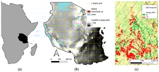
Figure 1.
(a) Tanzania inside eastern Africa, (b) TanDEM-X GlobalDEM with 1 × 1 degree grid which we further divided into a 2 arcmin grid, i.e., 30 gridlines per degree, and (c) TanDEM-X ChangeDEMlast and GEDI footprints for a selected area.
2.2. MODIS Land Cover
We derived land cover classes from the Moderate Resolution Imaging Spectroradiometer (MODIS) sensor. We used the MODIS Land Cover Type Product (MCD12Q1) and specifically Land Cover Type 1 (LC_Type1) which is generated for the International Geosphere-Biosphere Programme (IGBP). This land cover dataset has 17 classes, of which 15 were present in Tanzania. We used version 6.1 representing the year 2022. The spatial resolution was 500 m which we resampled to the TanDEM-X grid using the nearest neighbor. We downloaded the MODIS data from https://lpdaac.usgs.gov/products/mcd12q1v061/ on 2 July 2024. We used QGIS v. 3.34.11 and Python v. 3.8.6 for data management.
2.3. Global Forest Watch
To compare our method in the present study with conventional approaches, we obtained forest loss data from Global Forest Watch (GFW) [6]. We combined annual forest loss data from the eight years 2012–2019 to represent the same period as TanDEM-X change data, by using data that has ‘Lossyear’ version 2023-v11.1. As a loss area, we required that the area should have had at least 10% of tree cover prior to the deforestation by using the ‘treecover’ setting in GFW. For tree cover prior to the period 2002–2013 we used data for the year 2000, while for 2012–2019 we used year 2010. The spatial resolution of these data was 0.00025° which we resampled to the TanDEM-X grid using the nearest neighbor. We downloaded these data from https://www.globalforestwatch.org/ on 26 September 2024.
2.4. Tandem-X
We downloaded three TanDEM-X datasets, i.e., the GlobalDEM from around 2012 (Figure 1b), and the ChangeDEM which contained the two datasets first and last (Figure 1c) representing elevation changes from the former [21,22]. All these datasets had complete coverage of Tanzania. The former was generated from acquisitions taken over four years from December 2010 to January 2015 [23]. The two ChangeDEMs represented two alternative time periods. Since the majority of Tanzania was covered by more than one acquisition during the change period, the first was based on the oldest acquisition and the last on the newest. Each of these datasets was a mosaic from different acquisitions where each pixel had a time stamp. The GlobalDEM fitted reasonably well in time with NAFORMA field inventory and ChangeDEMlast fitted with the time of the GEDI acquisitions we used. We calculated the mean value of the ChangeDEMlast for the entire Tanzania and separately for each land cover type.
Prior to these analyses, we discarded a small fraction of pixels that we considered unreliable. In this filtering, we excluded pixels that had the following: (1) a change in DEM elevation > 25 m, (2) an estimated height change error > 1 m, and (3) MODIS land cover types 13 (Urban and Built-up Lands), 16 (Barren) or 17 (Water Bodies). We derived the height change error from the auxiliary datafile “Height Accuracy Indication (HAI)” which contained pixel-wise estimates of height change error based on the height errors of the initial DEM (GlobalDEM) and the last DEM [21]. These datasets had 1 arcsec spatial resolution, which corresponds to an area of 947 m2, or 30.7 m × 30.9 m, for a pixel in the center of Tanzania.
2.5. GEDI
GEDI is a spaceborne LiDAR generating ~25 m diameter full-waveform footprints (Figure 1c), which are processed into a suite of forest structure and topographic products. For each footprint we used the AGB variable, i.e., the Level 4A Predicted aboveground biomass density (agbd) [T/ha]. This variable had been obtained through parametric models based on simulated GEDI Level 2A (L2A) waveform relative height (RH) metrics from airborne LiDAR and ground-based measurements of AGB [24]. There were distinct models for various regions and plant functional types [25]. For Tanzania, the most used AGB models were the following: (1) Deciduous Broadleaf Trees (DBT), (2) Grasses, Shrubs, and Woodlands (GSW), and (3) Evergreen Broadleaf Trees (EBT) [26]. The R2 values of those models were 0.63, 0.86, and 0.64, respectively [26]. The predictor variables were RH50 and RH98, i.e., height relative to the ground elevation below which 50% and 98%, respectively, of waveform energy has been returned. We also used the elevation of the terrain, i.e., the Level 4A Elevation of the center of the lowest mode relative to reference ellipsoid (elev_lowestmode) [m].
We used the location of the center of each GEDI footprint to extract raster values from MODIS and TanDEM-X data. In this way, each GEDI footprint was supplemented by MODIS land cover class and TanDEM-X variables, i.e., DEM in 2012, the DEM change last and the height change error. We combined the data to generate new variables for the GEDI footprints, i.e., InSAR DEM in 2019 and InSAR height (IH) both in 2012 and 2019 (Figure 2):
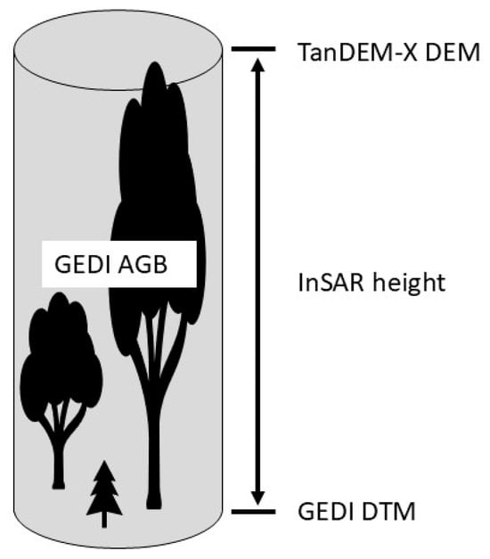
Figure 2.
The combination of TanDEM-X and GEDI data.
There was a total of 153 million available GEDI footprints over Tanzania which we reduced to 62 745 after filtering. First, we reduced this to 25 million by selecting footprints that had the following: (i) l2_quality_flag = 1 (high-fidelity waveforms suitable for height estimation); (ii) l4_quality_flag = 1 (suitable for AGBD estimation)); and (iii) sensitivity > 0.95 and geolocation/sensitivity_a2 > 0.95 (ability to penetrate dense canopy cover and having high confidence in relative height metrics) [24]. Secondly, we reduced this to 14.9 million by excluding footprints acquired after July 2021. Thirdly, we excluded footprints using the same filter as for TanDEM-X data (see above) and in addition those having |InSAR height| > 25 m. Finally, we generated a systematic and representative sample of GEDI footprints. The footprints were irregularly spaced over Tanzania (Figure 1c), and we laid out a 2 arcmin grid containing 69,182 points. For each grid point, we selected the nearest GEDI footprint within a maximum distance of the diagonal of 1 × 1 arcmin. This maximum distance was set to avoid the same footprint being duplicated for more than one grid point.
2.6. Conversion Factor
To estimate a conversion factor from InSAR height (IH) to AGB, we used the GEDI grid sample. Based on this, we calculated the conversion factor, k, separately for each MODIS land cover class, i = 1 … 11, based on proportionality, i.e., the ratio of the mean values of AGB and InSAR height as
2.7. Estimating AGB Change
The present method is the main method we pursued in this study, where we estimated net AGB change from change in TanDEM-X elevation and the conversion factor, i.e., as
where i = 1–11 are the eleven MODIS land cover classes having forest or woodlands, was mean InSAR elevation change for MODIS land cover type i, was the area, and was the conversion factor per m height change.
2.8. Comparison with Other Approaches
We compared our results with four alternative approaches. First, we used a conventional approach that corresponds to the IPCC Gain–Loss approach [4], however, without taking gain into account:
We obtained the loss area for a given MODIS class, , from GFW. We derived mean biomass stock per ha for each MODIS class, , as the mean GEDI derived AGB value of the grid sample of GEDI footprints for that MODIS class. This should correspond to emission factors that are often used in gain–loss calculations.
Secondly, we used a hybrid approach by combining the two approaches above. We used the same GFW loss areas as in Equation (5). However, we now multiplied these loss areas, L, by the mean TanDEM-X elevation change and the same conversion factors as used in Equation (4):
Thirdly, we compared this with the Tanzanian FREL (Forest Reference Emission Level) for the years 2002–2013 [27]. The FREL used the conventional approach as described above. The deforestation, or loss, data were based on a nationwide, wall-to-wall Landsat change analysis. The loss area was multiplied by emission factors calculated as the sum of three carbon stocks: Above Ground Carbon, Below Ground Carbon, and Dead Wood Carbon for each land cover type as given for mainland Tanzania by [28], supplemented by new data for Zanzibar, and finally multiplied by 3.667 to convert from carbon to CO2 equivalents [27]. In the present study, we recalculated this to AGB decrease. The dominating carbon fraction was the Above Ground Carbon, which can be recalculated to AGB by dividing it by 0.47. Hence, AGB and the emission factor in CO2 equivalents were strongly related. The ratio between them was fairly stable across land cover types with an area weighted mean value of 0.40. Hence, the FREL of 43.7 MT CO2e/year corresponded to a decrease of 17.5 MT AGB/year.
Finally, we redid the conventional approach (Equation (5)) for the FREL period 2002–2013. The rationale for this was to have one and the same method for the two periods 2002–2013 and 2012–2019 to clarify whether the differences between our present approach and the FREL could be attributed to differences in deforestation rate in the two periods or different calculation methods.
2.9. Uncertainty
We estimated the uncertainty of the estimated . We did this using the equation for standard deviation of a product, since we estimated as the product of the InSAR elevation change () and the conversion factor (k):
where and were the mean value and standard error of the conversion factor. In order to obtain these values for the conversion factor, we generated 4 more 2 arcmin grids, by moving the initial grid 0.5 arcmins towards the four cardinal directions (Figure 3). In this way, we obtained five nationwide samples, each having a mean AGB and InSAR height value, which resulted in five values of the conversion factor k. Here, for simplicity, we did not calculate this separately for each MODIS class but used the overall conversion factor.
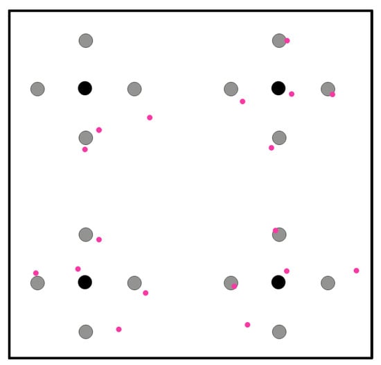
Figure 3.
The initial 2 arcmin grid (black) and the four additional grids (gray) as well as the selected nearest GEDI shots (violet), visualized for a small area.
To obtain mean and standard error for the height change, we used the ChangeDEMfirst and ChangeDEMlast as a sample of two datasets on change. The main uncertainty of a DEM change is likely to stem from temporal rather than spatial variation. This is so because each DEM may have its own vertical bias, and because InSAR height can be influenced by seasonal variations between leaf-on and leaf-off in some forest types such as a miombo woodland. These two datasets covered different lengths in time, and to make them comparable we recalculated them to annual height change. We did that by calculating the length of the time period for each pixel as the difference between the date of the ChangeDEM and the mean date of the GlobalDEM. Based on this we first obtained the period length given as the number of days for each pixel. Secondly, based on this we obtained the annual height change for each pixel, which we averaged over the entire area.
The mean values of k and differed somewhat from their initial values as described above, i.e., based on the initial 2 arcmin grid and based on the ChangeDEMlast; however, we here retained only the estimated uncertainty, .
2.10. Validation
Estimated AGB change at the national level cannot be validated, as the true value is unknown. However, we carried out supplementary analyses that could support or corroborate the results. Firstly, we compared our AGB change estimates with GFW and the geography of protected areas. We divided the Tanzanian forest and wooded land into two categories based on GFW, i.e., loss and no-loss. We did this by combining the annual loss dataset for the eight years 2012–2019. We calculated the mean InSAR elevation change and estimated mean AGB change for these two categories. Furthermore, we divided the land area of Tanzania into two categories, protected and unprotected. We then compared our AGB change estimates with these categories. The protected areas made up 29% of the forest and wooded land area. Therefore, understanding biomass dynamics within protected areas is important for interpreting broader temporal trends in Tanzania’s forest landscape.
Secondly, we used the combination of TanDEM-X and GEDI to estimate mainland Tanzania’s AGB stock in 2012 and compared that to the field-plot-based estimates of AGB stock data from NAFORMA [28]. A national high quality DTM does not exist for Tanzania, and hence our approach was to estimate this based on a sample estimate using the GEDI grid sample described above. As the GEDI footprints had a DTM variable, we could derive InSAR height and recalculate that to AGB for each footprint. We estimated the national scale AGB stock from this sample as
where .
3. Results
3.1. InSAR Height Change
The mean eight-year InSAR height change was a decrease of 2.2 cm (Table 1). The change varied between MODIS land cover types. The overall decrease was mainly a result of a decrease in savannahs, which was considerable (8.7 cm) and covered a large fraction of the total area (46%). The grasslands also contributed considerably in the same way. Contrary to this were the three most forested land cover types, i.e., Evergreen and Deciduous Broadleaf Forests and Mixed Forests appearing in the three uppermost rows in Table 1, where there was an increase in InSAR height, indicating a net growth and gain. However, these three land cover types covered only 6% of the area and had a small influence on the national statistics.

Table 1.
Means and totals grouped by MODIS land cover types, as well as for entire Tanzania at bottom. is mean InSAR height decrease, and Area is the area of each MODIS class. is mean InSAR height above ground, is mean AGB and k is the conversion factor for each MODIS class based on the GEDI grid sample. The last row (bold) contains means and totals for entire Tanzania.
3.2. Conversion Factor
The conversion factor had an overall value of 13.9 T/ha/m based on the entire GEDI footprint grid sample. It varied between MODIS land cover types from 11.3 T/ha/m to 137.6 T/ha/m (Table 1). The Grasslands and Savannas land cover classes covered large areas (Figure 4). The influence of the former was still minor, because the two variables AGB and InSAR height had small values. The conversion factor of the latter was 13.3, and this class had a large influence on the total statistics. Most of the land cover types had similar values in the range 11.3–20.7. The forest land cover types having a mean AGB > 40 T/ha had somewhat smaller conversion factors than the overall value of 13.9. On the other end of the scale, the two classes Closed Shrublands and the Cropland/Natural Vegetation Mosaics had very high values, i.e., 137.6 and 113.3, respectively. However, these classes had little influence on total statistics because they had small values both for AGB and InSAR height, and they covered small areas.
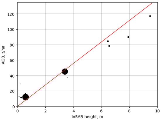
Figure 4.
Mean AGB plotted against mean InSAR height for each of the MODIS land cover types, as well as the overall conversion factor of 13.9 T/ha/m given as a red line. The markers are proportional in size to the area of the respective MODIS land cover type, where the two dominating types are nos. 10 (Grasslands, left) and 9 (Savannas, right).
3.3. Biomass Change
A countrywide map of estimated AGB change provided a geographic overview with lots of details (Figure 5a). This dataset makes up a valuable basis for further analysis of causes as well as forest policy and management. The dataset can be interpreted together with other datasets such MODIS land cover classes (Figure 5b), topography (Figure 1b), protected forest areas (see below), and distance to urban areas. Such geographic analyses were not part of the objectives of the present study. However, we can briefly note that both increases and decreases occur scattered over the country. We see patches of increase and of decrease, and they occur both in forests and in other wooded land.
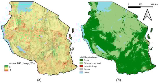
Figure 5.
Tanzanian map of (a) estimated annual AGB change and (b) MODIS land cover classes grouped into categories. We selected ±5 T/ha for the color scale in (a) corresponding to the 5th to 96th percentile values.
With the present approach using TanDEM-X and GEDI, and aggregating statistics across MODIS land cover classes, we obtained an estimate of the annual AGB decrease to be 3.0 MT during the eight years from the beginning of 2012 to the end of 2019 (Table 1 and Table 2). This represents the net change, i.e., the difference between gains and losses.
Table 2.
Estimated annual AGB change for five alternatives based on different methods (equations numbers) and different time periods.
3.4. Comparison with Other Approaches
As expected, the other approaches resulted in higher biomass losses because they are loss-only estimates. However, they were considerably higher, and this indicates that considerable gains are also ongoing. By comparing the present approach with the conventional and hybrid, i.e., the three uppermost rows of Table 2, we obtain an estimated annual gain of 6.2–6.6 MT. The loss area was 2.0 million ha, corresponding to 2.3% of the land area, which means that the gain occurred in the remaining 97.7% of the area. As mentioned above, a net gain appeared to be the case in the Evergreen and Deciduous Broadleaf Forests and Mixed Forests.
The conventional and hybrid approaches yielded similar results. This means that AGB before deforestation corresponded well to the decrease in InSAR height. The mean InSAR elevation decrease on the loss area was 2.45 m, which corresponds to an AGB decrease of 34.1 T/ha. This is like the mean AGB on this area prior to deforestation, i.e., 39.0 T/ha. These numbers represent the eight-year period.
The AGB decrease recalculated from FREL was much higher than we obtained with the present approach, i.e., about six times higher. The numbers are not directly comparable, as the periods are different and the former represents loss only while the latter represents net change. However, with our conventional approach based on GFW loss area and GEDI-based AGB densities we see that the annual loss in the two periods was quite close. Hence, differences in forest loss between the two periods are of minor importance as an explanation for the difference. The FREL-based AGB decrease was 2.5 times higher than we obtained with the conventional approach for the same period as FREL. Further analyses showed that the difference was mainly due to a large difference in estimated deforestation area, which was 2.3 times higher in FREL than with GFW. In addition, the mean AGB stock per ha was 9% higher in FREL than we obtained with GEDI.
3.5. Uncertainty
The annual AGB density change during the eight-year period 2012–2019 was estimated to be −0.035 ± 0.028 T/ha. The estimated −0.035 T/ha was the product of the mean change in the ChangeDEMlast = −0.020 m and the conversion factor k = 13.9 T/ha/m and divided by eight years. This was combined with the uncertainty estimate given as a standard error which was estimated based on the uncertainties of and the conversion factor, k (Table 3).
Table 3.
Uncertainty of annual and the conversion factor, k, as input factors for estimating uncertainty of .
With these input parameters, the random error on the annual was calculated from Equation (7) as the square root of the sum of three elements:
This equation was dominated by the last element, , and the equation could be reduced to:
Aggregated over Tanzania the estimated AGB change was −2.96 ± 2.44 MT per year, based on a forest area of 86.5 million ha.
3.6. Validation
Firstly, a visual inspection revealed that the areas having a decrease in the TanDEM-X DEM corresponded fairly well with the GFW loss pixels (Figure 6). This was also the case for protected areas. A large share of pixels inside protected areas had increasing InSAR elevation, indicating forest growth. Contrary to this were the areas in between the protected areas where pixels having a decrease in InSAR elevation dominated (Figure 6). The borders between these categories were in many cases sharp. However, this was not always the case, and some protected areas appeared to have been severely affected by logging. There was a considerable difference in AGB change between protected areas and unprotected. For the former, we estimated a mean net increase in AGB of 3.9 MT/yr, while the latter had a mean decrease, i.e., −6.9 MT/yr. This made up a net change of −3.0 MT/yr.
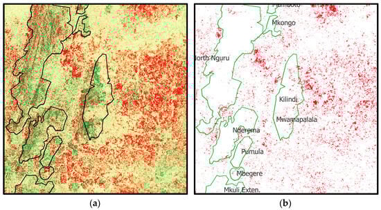
Figure 6.
Example area with protected areas (black outlines) and the in-between unprotected areas from central Tanzania (−5.57°S, 37.57°E) showing changes in 2012–2019; (a) TanDEM-X elevation changes scaled green–red ±5 m; (b) GFW loss (red).
Secondly, with the GEDI and TanDEM-X data we obtained an estimated AGB stock for Tanzania mainland in 2012 that was almost identical to the one obtained with the NAFORMA field inventory plots (Table 4).
Table 4.
Estimated AGB stock for the year 2012 based on TanDEM-X and GEDI including mean biomass density and total for mainland Tanzania, and in comparison, the estimate based on the national forest inventory field plots (NAFORMA).
4. Discussion
This study demonstrated that forest biomass’ change over time can be estimated based on X-band across-track, single-pass interferometry, i.e., InSAR elevation change from TanDEM-X, and a conversion from elevation change to AGB change based on a combination of TanDEM-X and GEDI. In addition to mean values for entire Tanzania, the method can be used to show maps of changes. Furthermore, in addition to mean values, the method provided results for both gain and loss of AGB. The advantage of this is that it generates the basis for a better understanding of forest dynamics. It is valuable to see that for Tanzania as a country in the tropics, where deforestation is a well-known and severe environmental issue, there are considerable AGB gains. These gains are normally not picked up, and if they are, only at rare intervals like decades. This study showed that AGB gain mainly occurred in the three MODIS forest classes having the highest standing AGB, i.e., Evergreen and Deciduous Broadleaf and Mixed Forests, and in protected areas. The AGB loss mainly occurred in savannas and grasslands outside protected areas. This shows how the present method can provide valuable input to national forest policy.
To obtain the conversion factors, we used proportionality, i.e., the ratio between mean AGB and mean InSAR height. An alternative would be to use ordinary least squares in the form of a linear regression model. However, there is one problem with that. Such a model will have an intercept. In most cases the intercept will have a positive sign, and this will result in predicted AGB values > 0 for areas without trees, i.e., when InSAR height is zero. In this way, the model will be counterintuitive and not suitable for operational applications. In addition, this would prevent the method to be used in areas without a DTM. Another alternative would be to use a no-intercept regression model. However, the problem with that is that such a model represents a biased estimator. The mean value of the predictions will not be equal to the mean value of the ground truth. Based on this and our experience from several similar studies, we selected proportionality as the preferred model. However, the model choice is not critical, as the three model types can generate similar conversion factors. Solberg et al. [20] obtained the conversion factor 12.1 T/ha/m with proportionality, 11.8 with ordinary OLS regression, and 12.0 with OLS no-intercept regression.
GEDI appears to be a good alternative to forest biomass data from field inventory. Field inventories, like national forest inventories, are rare in the tropics. GEDI makes up an alternative to costly and time-consuming field work in remote and low-accessibility areas. The role of GEDI in our method is to calibrate the conversion from InSAR elevation change to AGB change. One way to evaluate the GEDI data is to compare our obtained conversion factors with those from earlier studies based on field inventory. We see from our results that the conversion factors we obtained in the present study are consistent with earlier studies, and they were also quite stable across different MODIS land cover types. The overall conversion factor across land cover types was 13.9 T/ha/m, which is close to what has been found in other studies. In Tanzania there are two intensively studied forest areas, having field inventory plots and airborne laser scanning. One is the Liwale area in the southeast with miombo woodland. This area was dominated by the MODIS land cover classes Savannas, Deciduous Broadleaf Forests, and Mixed Forests, and in this study, we obtained the conversion factors 13.3, 13.1, and 11.3 T/ha/m, respectively, for them. Three earlier studies using various versions of field inventory plot data found 14.1 [14], 11.9 [16], and 14.0 T/ha/m [20]. Using GEDI instead of field inventory resulted in 12.1 T/ha/m [20].
A second study area is Amani, located in East Usambara Mountains in the northeast and has exceptionally high AGB density values ranging up to >1000 T/ha. It was dominated by the MODIS land cover class Evergreen Broadleaf Forests for which we obtained a conversion factor of 12.3 T/ha/m. Although this value appears to be reasonable because it is close to other conversion factors values, it is clearly lower than the value 18.4 T/ha/m that has been found based on field plots in Amani [15]. There are several possible reasons for this difference. First, it is possible that there is a limitation with GEDI. This forest type can have extremely high AGB. Perhaps the GEDI LiDAR pulses have problems penetrating down to the terrain in this dense forest with tall trees, leading to biased AGB estimates here. Secondly, there is much sloping terrain in that mountain area, which possibly leads to SAR-specific geometric problems, including differences in obtained InSAR height between hillsides facing towards the sensor and hillsides facing away. Thirdly, the MODIS land cover type Evergreen Broadleaf Forests did not cover the same area as the Amani study area with its field inventory plots. Altogether, the causes for the discrepancy between the conversion factors 12.3 T/ha/m using GEDI and TanDEM-X in the present study and 18.4 T/ha/m found in another study based on field plots and TanDEM-X [15] are unknown. However, the Evergreen Broadleaf Forests covers only 2% of Tanzania’s land area, and a bias on the conversion factor here has minor influence on national statistics. Still, we recommend a separate study to clarify the causes. For other forest types, conversion factors have been found to be 14.9 in a Norway spruce forest in Norway [29] and 13.0 T/ha/m based on published data from a tropical forest in Brazil [25]. The majority of conversion factors found in the present study appears to be close to an almost generic value across forest types of 12–14 T/ha/m, with a possible exception for the Amani area.
The alternative approaches for AGB change at the national scale were consistent and supplemented each other. While the present method provided an estimated annual net AGB change of −3.0 MT, the conventional and hybrid approaches resulted in an estimated annual loss of about 9 MT. Hence, the annual gain can be derived as about 6 MT. The similarity between the conventional and hybrid approaches makes up a validation of the method; they both use as input the loss pixels from GFW, and for those pixels the AGB loss was similar either when calculated as a complete loss of standing AGB prior to logging taken as the mean AGB of the actual MODIS land cover classes, or calculated as the mean InSAR elevation decrease multiplied by the conversion factor. However, the Tanzanian FREL appeared to be an overestimation of the greenhouse gas emissions from forest loss. This was mainly a result of a very large estimate of the deforestation area, and this shows one weakness of using the conventional approach for FREL and forest loss statistics: estimation of the loss area from optical satellite imagery is uncertain.
In addition to the correspondence between different approaches and the similarity with conversion factors found earlier, our findings are also supported in other ways. First, GFW loss pixels and InSAR elevation change corresponded well with each other. The GFW loss pixels and that of decreasing InSAR elevation had a similar spatial distribution. This was particularly evident when taking protected areas into account, where GFW loss and decreasing InSAR elevation dominated in the unprotected areas. The protected areas made up 29% of Tanzania’s land area, and hence, the temporal changes seen here have a large influence on national statistics on forest loss and CO2 emissions. Finally, our estimate of national mainland AGB stock in 2012 was almost identical to the estimate generated by Tanzania’s NAFORMA field based national forest inventory [28]. Our estimate was 2.76 MT while the NAFORMA estimate was 2.69 MT, i.e., we had a 2% overestimation. Any further validation of our results was not feasible. The main ground truth dataset in Tanzania is the NAFORMA field inventory plots. However, for the present study that dataset was not available, and they represent only one point in time. An exception is for a part of the Liwale study area, where NAFORMA plots have AGB data from repeated field inventory. Those data on AGB change were used by Solberg, Bollandsås, Gobakken, Næsset, Basak, and Duncanson [20] to validate the present method in that smaller area.
One source of errors is that the datasets were not completely aligned in time. In particular, the temporal mismatch varied from pixel to pixel in the TanDEM-X datasets. However, these errors are of negligible importance for the results on the national scale. The mean InSAR height across Tanzania based on the representative grid sample was 2.38 m with the GlobalDEM around 2012 and 2.37 m based on the same data and ChangeDEMlast around 2019. This means a net decrease of only 0.3% of standing AGB occurred during those eight years. Hence, even though there has been a net loss of AGB over time, this has been small compared to the standing AGB.
When the GEDI AGB estimator was trained [26], three important Tanzanian datasets were used, i.e., the field plots of NAFORMA and field plots and airborne laser scanning data for the two intensively studied areas Liwale and Amani. Hence, GEDI predictions for Tanzania may be less erroneous than what can be expected in other countries.
There is today a problem for a practical implementation of the present method for FREL and REDD+ MRV reporting. There is a lack of suitable data for the coming years, as there is a lack of across-track, single-pass interferometers. The practical implementation could have started at the onset of the TanDEM-X mission or with support for the planned TanDEM-L mission. By now, TanDEM-X is close to its termination. The commercial aspect of that mission has also prevented routine acquisitions on the global scale, and although global datasets are now available, this is the case only for a few points in time. Conventional, optical satellite imagery has during the last 10–15 years received most attention at the expense of suitable SAR interferometers. There are, however, some missions that have the technical capability to provide such data. One is the European Earth Explorer C-band mission Harmony, which is scheduled to go in across-track formation for part of its time, although this time share is small. Another mission is the Chinese Hongtu-1 X-band mission, which with one active and three passive receivers provides several across-track baselines simultaneously, and has the technical potential to improve performance beyond TanDEM-X [30]. However, this sensor is mainly set up to provide national data takes in China. There are other missions to be mentioned in this context, such as the P-band BIOMASS mission and the L-band NISAR mission, which both provide repeat-pass interferometry. With this study, we want to support initiatives for launching new across-track, single-pass SAR interferometers in the coming years.
5. Conclusions
In conclusion, an across-track, single-pass interferometer such as TanDEM-X and a space lidar such as GEDI can be combined for deriving reliable temporal change in AGB at large scales such as a country. An important advantage of the method is that it is not required to have a representative field inventory plot network nor a full coverage DTM. The estimated forest biomass change can further be used for estimating carbon dioxide emission data for setting up a FREL or regular REDD+ reporting. This is an alternative to the conventional approach where deforestation data (“activity data”) are combined with biomass density data (“emission factors”). The present method makes up a supplement to the conventional method, by having the net change, which can be split into gain and loss. We recommend further analyses of dense tropical forests having exceptionally high biomass values.
Author Contributions
Conceptualization, S.S. and B.G.; methodology, S.S., B.G., L.I.D. and P.B.; software, S.S., L.I.D. and P.B.; validation, S.S.; formal analysis, S.S.; investigation, S.S.; resources, all authors; writing—original draft, all authors; project administration, S.S.; funding acquisition, S.S. All authors have read and agreed to the published version of the manuscript.
Funding
This research was jointly funded by the Norwegian Space Agency contract no. 20142VNA and the Norwegian Institute of Bioeconomy Research through the project “Biomass change in forest in Tanzania 2012–2020”.
Data Availability Statement
The original contributions presented in this study are included in the article. Further inquiries can be directed to the corresponding author.
Acknowledgments
We acknowledge our NIBIO colleague Nils Egil Søvde for data management and calculations. The authors have reviewed and edited the output and take full responsibility for the content of this publication.
Conflicts of Interest
The authors declare no conflicts of interest.
References
- Le Toan, T.; Quegan, S.; Davidson, M.; Balzter, H.; Paillou, P.; Papathanassiou, K.; Plummer, S.; Rocca, F.; Saatchi, S.; Shugart, H. The Biomass Mission: Mapping Global Forest Biomass to Better Understand the Terrestrial Carbon Cycle. Remote Sens. Environ. 2011, 115, 2850–2860. [Google Scholar] [CrossRef]
- IPCC. Climate Change 2014: Mitigation of Climate Change. Contribution of Working Group III to the Fifth Assessment Report of the Intergovernmental Panel on Climate Change; Edenhofer, O., Pichs-Madruga, R., Sokona, Y., Farahani, E., Kadner, S., Seyboth, K., Adler, A., Baum, I., Brunner, S., Eickemeier, P., et al., Eds.; Cambridge University Press: Cambridge, UK; New York, NY, USA, 2014. [Google Scholar]
- UNFCCC. Decision 2/CP. 13: Reducing Emissions from Deforestation in Developing Countries: Approaches to Stimulate Action; United Nations Framework Convention on Climate Chgange: Bonn, Germany, 2007; Available online: http://unfccc.int/resource/docs/2007/cop13/eng/06a01.pdf (accessed on 19 September 2014).
- IPCC. 2006 Ipcc Guidelines for National Greenhouse Gas Inventories: Volume 4—Agriculture, Forestry and Other Land Use. Prepared by the National Greenhouse Gas Inventories Programme; Eggleston, H.S., Buendia, L., Miwa, K., Ngara, T., Tanabe, K., Eds.; IPCC: Kanagawa, Japan, 2006.
- Houghton, R.A.; House, J.I.; Pongratz, J.; van der Werf, G.R.; DeFries, R.S.; Hansen, M.C.; Le Quere, C.; Ramankutty, N. Carbon Emissions from Land Use and Land-Cover Change. Biogeosciences 2012, 9, 5125–5142. [Google Scholar] [CrossRef]
- Hansen, M.C.; Potapov, P.V.; Moore, R.; Hancher, M.; Turubanova, S.A.; Tyukavina, A.; Thau, D.; Stehman, S.V.; Goetz, S.J.; Loveland, T.R.; et al. High-Resolution Global Maps of 21st-Century Forest Cover Change. Science 2013, 342, 850–853. [Google Scholar] [CrossRef] [PubMed]
- Baccini, A.; Goetz, S.J.; Walker, W.S.; Laporte, N.T.; Sun, M.; Sulla-Menashe, D.; Hackler, J.; Beck, P.S.A.; Dubayah, R.; Friedl, M.A.; et al. Estimated Carbon Dioxide Emissions from Tropical Deforestation Improved by Carbon-Density Maps. Nat. Clim. Chang. 2012, 2, 182–185. [Google Scholar] [CrossRef]
- Saatchi, S.; Harris, N.; Brown, S.; Lefsky, M.; Mitchard, E.; Salas, W.; Zutta, B.; Buermann, W.; Lewis, S.; Hagen, S.; et al. Benchmark Map of Forest Carbon Stocks in Tropical Regions across Three Continents. Proc. Natl. Acad. Sci. USA 2011, 108, 9899–9904. [Google Scholar] [CrossRef]
- Mitchard, E.T.A.; Feldpausch, T.R.; Brienen, R.J.W.; Lopez-Gonzalez, G.; Monteagudo, A.; Baker, T.R.; Lewis, S.L.; Lloyd, J.; Quesada, C.A.; Gloor, M.; et al. Markedly Divergent Estimates of Amazon Forest Carbon Density from Ground Plots and Satellites. Glob. Ecol. Biogeogr. 2014, 23, 935–946. [Google Scholar] [CrossRef]
- Avitabile, V.; Herold, M.; Henry, M.; Schmullius, C. Mapping Biomass with Remote Sensing: A Comparison of Methods for the Case Study of Uganda. Carbon Balance Manag. 2011, 6, 7. [Google Scholar] [CrossRef]
- Solberg, S.; Astrup, R.; Gobakken, T.; Næsset, E.; Weydahl, D.J. Estimating Spruce and Pine Biomass with Interferometric X-Band Sar. Remote Sens. Environ. 2010, 114, 2353–2360. [Google Scholar] [CrossRef]
- Krieger, G.; Moreira, A.; Fiedler, H.; Hajnsek, I.; Werner, M.; Younis, M.; Zink, M. Tandem-X: A Satellite Formation for High-Resolution Sar Interferometry. IEEE Trans. Geosci. Remote Sens. 2007, 45, 3317–3341. [Google Scholar] [CrossRef]
- Solberg, S.; Astrup, R.; Breidenbach, J.; Nilsen, B.; Weydahl, D. Monitoring Spruce Volume and Biomass with Insar Data from Tandem-X. Remote Sens. Environ. 2013, 139, 60–67. [Google Scholar] [CrossRef]
- Solberg, S.; Gizachew, B.; Næsset, E.; Gobakken, T.; Bollandsås, O.M.; Mauya, E.W.; Olsson, H.; Malimbwi, R.; Zahabu, E. Monitoring Forest Carbon in a Tanzanian Woodland Using Interferometric Sar: A Novel Methodology for Redd+. Carbon Balance Manag. 2015, 10, 14. [Google Scholar] [CrossRef]
- Solberg, S.; Hansen, E.H.; Gobakken, T.; Naesset, E.; Zahabu, E. Biomass and Insar Height Relationship in a Dense Tropical Forest. Remote Sens. Environ. 2017, 192, 166–175. [Google Scholar] [CrossRef]
- Puliti, S.; Solberg, S.; Næsset, E.; Gobakken, T.; Zahabu, E.; Mauya, E.; Malimbwi, R.E. Modelling above Ground Biomass in Tanzanian Miombo Woodlands Using Tandem-X Worlddem and Field Data. Remote Sens. 2017, 9, 984. [Google Scholar] [CrossRef]
- Karila, K.; Yu, X.; Vastaranta, M.; Karjalainen, M.; Puttonen, E.; Hyyppä, J. Tandem-X Digital Surface Models in Boreal Forest above-Ground Biomass Change Detection. ISPRS J. Photogramm. Remote Sens. 2019, 148, 174–183. [Google Scholar] [CrossRef]
- Dubayah, R.; Armston, J.; Healey, S.P.; Bruening, J.M.; Patterson, P.L.; Kellner, J.R.; Duncanson, L.; Saarela, S.; Ståhl, G.; Yang, Z. Gedi Launches a New Era of Biomass Inference from Space. Environ. Res. Lett. 2022, 17, 095001. [Google Scholar] [CrossRef]
- Solberg, S.; May, J.; Bogren, W.; Breidenbach, J.; Torp, T.; Gizachew, B. Interferometric Sar Dems for Forest Change in Uganda 2000–2012. Remote Sens. 2018, 10, 228. [Google Scholar] [CrossRef]
- Solberg, S.; Bollandsås, O.M.; Gobakken, T.; Næsset, E.; Basak, P.; Duncanson, L.I. Biomass Change Estimated by Tandem-X Interferometry and Gedi in a Tanzanian Forest. Remote Sens. 2024, 16, 861. [Google Scholar] [CrossRef]
- Lachaise, M.; Schweißhelm, B. Tandem-X 30m dem Change Maps Product Description, Issue Public Document Td-Gs-Ps-0216 Issue 1.0, 12.10.2023; 2023. Available online: https://geoservice.dlr.de/web/dataguide/tdm30/pdfs/TD-GS-PS-0216_TanDEM-X_30m_DEM_Change_Maps_Product_Description_1.0.pdf (accessed on 15 June 2025).
- Lachaise, M.; González, C.; Rizzoli, P.; Schweiβhelm, B.; Zink, M. The New Tandem-X Dem Change Maps Product. In Proceedings of the IGARSS 2022—2022 IEEE International Geoscience and Remote Sensing Symposium, Kuala Lumpur, Malaysia, 17–22 July 2022; pp. 5432–5435. [Google Scholar]
- Gonzalez, C.; Bueso-Bello, J.L. Tandem-X 30m Edited Dem Product Description; German Aerospace Center (DLR): Köln, Germany, 2023. [Google Scholar]
- Kellner, J.R.; Armston, J.; Duncanson, L. Algorithm Theoretical Basis Document for Gedi Footprint Aboveground Biomass Density. Earth Space Sci. 2023, 10, e2022EA002516. [Google Scholar] [CrossRef]
- Neeff, T.; Dutra, L.V.; dos Santos, J.R.; Freitas, C.D.; Araujo, L.S. Tropical Forest Measurement by Interferometric Height Modeling and P-Band Radar Backscatter. For. Sci. 2005, 51, 585–594. [Google Scholar] [CrossRef]
- Duncanson, L.; Kellner, J.R.; Armston, J.; Dubayah, R.; Minor, D.M.; Hancock, S.; Healey, S.P.; Patterson, P.L.; Saarela, S.; Marselis, S.; et al. Aboveground Biomass Density Models for Nasa’s Global Ecosystem Dynamics Investigation (Gedi) Lidar Mission. Remote Sens. Environ. 2022, 270, 112845. [Google Scholar] [CrossRef]
- The United Republic of Tanzania. Tanzania’s Forest Reference Emission Level Submission to the UNFCCC. 2017. p. 54. Available online: https://redd.unfccc.int/media/2017_submission_frel_tanzania.pdf (accessed on 4 April 2024).
- Mauya, E.W.; Mugasha, W.A.; Njana, M.A.; Zahabu, E.; Malimbwi, R. Carbon Stocks for Different Land Cover Types in Mainland Tanzania. Carbon Balance Manag. 2019, 14, 4. [Google Scholar] [CrossRef]
- Solberg, S.; Næsset, E.; Gobakken, T.; Bollandsås, O.-M. Forest Biomass Change Estimated from Height Change in Interferometric Sar Height Models. Carbon Balance Manag. 2014, 9, 5. [Google Scholar] [CrossRef]
- Deng, Y.; Zhang, H.; Liu, K.; Wang, W.; Ou, N.; Han, H.; Yang, R.; Ren, J.; Wang, J.; Ren, X.; et al. Hongtu-1: The First Spaceborne Single-Pass Multibaseline Sar Interferometry Mission. IEEE Trans. Geosci. Remote Sens. 2025, 63, 5202518. [Google Scholar] [CrossRef]
Disclaimer/Publisher’s Note: The statements, opinions and data contained in all publications are solely those of the individual author(s) and contributor(s) and not of MDPI and/or the editor(s). MDPI and/or the editor(s) disclaim responsibility for any injury to people or property resulting from any ideas, methods, instructions or products referred to in the content. |
© 2025 by the authors. Licensee MDPI, Basel, Switzerland. This article is an open access article distributed under the terms and conditions of the Creative Commons Attribution (CC BY) license (https://creativecommons.org/licenses/by/4.0/).