Article

Satellite-Based Prediction of Water Turbidity Using Surface Reflectance and Field Spectral Data in a Dynamic Tropical Lake

by
Elsa Pereyra-Laguna
1,
Valeria Ojeda-Castillo
2,
Enrique J. Herrera-López
1,
Jorge del Real-Olvera
3,
Leonel Hernández-Mena
3,
Ramiro Vallejo-Rodríguez
3 and
Jesús Díaz
4,*
1
Laboratory for Innovation in Bioelectronics and Artificial Intelligence, LINBIA, Industrial Biotechnology, Center for Research and Assistance in Technology and Design of the State of Jalisco, 1227 Camino Arenero, El Bajío del Arenal, Zapopan 45019, Mexico
2
Universidad de Guadalajara, Av. Juárez No. 976, Colonia Centro, Guadalajara 44100, Mexico
3
Environmental Technology Unit, Center for Research and Assistance in Technology and Design of the State of Jalisco, 800, Normalistas Ave., Colinas de la Normal, Guadalajara 44270, Mexico
4
Data and Digital Cartography Laboratory, Analytical and Metrological Services Unit, Center for Research and Assistance in Technology and Design of the State of Jalisco, 800, Normalistas Ave., Colinas de la Normal, Guadalajara 44270, Mexico
*
Author to whom correspondence should be addressed.
Remote Sens. 2025, 17(15), 2595; https://doi.org/10.3390/rs17152595
Submission received: 4 May 2025 / Revised: 22 July 2025 / Accepted: 24 July 2025 / Published: 25 July 2025

Abstract

Turbidity is a crucial parameter for assessing the ecological health of aquatic ecosystems, particularly in shallow tropical lakes that are subject to climatic variability and anthropogenic pressures. Lake Chapala, the largest freshwater body in Mexico, has experienced persistent turbidity and sediment influx since the 1970s, primarily due to upstream erosion and reduced water inflow. In this study, we utilized Landsat satellite imagery in conjunction with near-synchronous in situ reflectance measurements to monitor spatial and seasonal turbidity patterns between 2023 and 2025. The surface reflectance was radiometrically corrected and validated using spectroradiometer data collected across eight sampling sites in the eastern sector of the lake, the area where the highest rates of horizontal change in turbidity occur. Based on the relationship between near-infrared reflectance and field turbidity, second-order polynomial models were developed for spring, fall, and the composite annual model. The annual model demonstrated acceptable performance (R2 = 0.72), effectively capturing the spatial variability and temporal dynamics of the average annual turbidity for the whole lake. Historical turbidity data (2000–2018) and a particular case study in 2016 were used as a reference for statistical validation, confirming the model’s applicability under varying hydrological conditions. Our findings underscore the utility of empirical remote-sensing models, supported by field validation, for cost-effective and scalable turbidity monitoring in dynamic tropical lakes with limited monitoring infrastructure.

1. Introduction

Understanding the equilibrium state of aquatic systems is essential for informed decision-making and the preservation of the health of dependent organisms [1,2]. This is particularly relevant in tropical and subtropical regions, which are among the most sensitive to climate change [3]. In this context, we examine Lake Chapala, a shallow water body located in the subtropical region of western Mexico. It is the largest lake in Mexico, with a maximum depth of 10.5 m [4]. The lake’s depth and volume were affected by reduced flow in the late 1970s, attributed to dam construction on the Lerma River [5,6]. Since that time, average lake levels have fluctuated around 60% of their actual maximum capacity (7897 Mm3), which is significantly below the historical highs recorded in 1926 (9663 Mm3) (https://www.ceajalisco.gob.mx/contenido/chapala/, accessed on 4 May 2025).
The current conditions expose the lake to atypical climatic phenomena, such as droughts. Over the past two decades, a semi-permanent drought classified as anomalous dry (D0) has been observed in western Mexico, characterized by periods lasting two to five years, interrupted by brief intervals (https://droughtmonitor.unl.edu/NADM/Statistics.aspx/, accessed on 4 May 2025). The severity of these droughts has progressively intensified, reaching an exceptional classification (D4) in extensive areas of western Mexico, including the Lake Chapala region [7]. This climatic condition induces significant fluctuations in the water volume of rivers and lakes and adversely affects water quality, leading to substantial alterations in natural processes. Consequently, addressing water quality in response to these phenomena necessitates an immediate response, involving real-time monitoring of key indicators such as turbidity.
Management strategies for large aquatic systems face significant operational challenges in monitoring water quality, necessitating considerable investments in financial and human resources. This traditional approach inherently offers limited spatial coverage and yields spatially discrete and temporally asynchronous measurements. Environmental remote sensing for water quality assessment offers an alternative method to address the limitations of conventional monitoring. This innovative approach utilizes alternative methods and technological tools that complement direct water quality assessment. The spatial coverage provided by satellite imagery offers a comprehensive and instantaneous view of the optical properties of water, which can assist in characterizing the physical, chemical, or biological phenomena occurring within a water body, thereby supporting information from discrete records. Furthermore, the periodic satellite pass facilitates the assessment of any phenomenon in near real time and provides a historical dataset for analyzing trends, patterns, or tracking changes over time, enabling a rapid response to pollution events.
With 52 years of data collection, the continuous research and rigorous quality protocols implemented by the Landsat program have established it as one of the most robust platforms, offering a diverse array of products. This has resulted in several product enhancements, including (1) improved image quality, (2) a standardized revisit period over the same site every 16 days, (3) satellite synchronization (e.g., Landsat 8 and 9) to double the data acquisition, thereby increasing the temporal resolution from 16 to 8 days, (4) standardized scene size, and (5) consistent spatial coverage between scenes. Despite their spatial resolution of 30 m per pixel, the attributes of Landsat products render them an optimal choice for research on the optical properties of water bodies and their spatiotemporal variations. Notably, the adjustment of the detector range (from 760–900 nm in Landsat 5 to 850–880 nm in Landsat 8 and 9) to measure the near-infrared spectral response is crucial for conducting research on turbidity linked to inorganic matter in inland water bodies.
The estimation of water quality parameters through optical properties and remote sensing is a well-established practice [8]. Three methodological approaches are employed to model water properties in various aquatic environments: empirical, analytical, and machine learning [9,10]. Herein, we succinctly outline the advantages and limitations of these models as discussed by these authors. Empirical models are extensively utilized due to their simplicity and minimal computational demands. Nonetheless, their predictive capability is constrained by the range of values used for their parameterization and the dynamics of the water body, limiting their applicability across different water bodies. Analytical models are based on the inherent optical properties of water (IOPs) and the atmosphere, which are independent of the ambient light field. These models are infrequently applied in complex water bodies due to the challenges associated with modeling interactions among various water components, and their application as a singular model to optically heterogeneous water bodies requires substantial in situ validation data. Conversely, machine learning approaches, while inherently empirical, are distinguished by their capacity to function in a multidimensional space. These algorithms can produce generalizable models that capture the intricate nonlinear relationships between remotely sensed reflectance and water quality parameters. However, they are heavily reliant on the range and context of data used for model training, the parameterization, and the volume of training data available, which may result in overfitting, particularly in models with numerous input variables subject to collinearity.
The current literature on water quality assessment through remote sensing in Lake Chapala and its surrounding water bodies is relatively limited, and existing studies present certain limitations that this research seeks to address. Several studies have estimated water quality indices or parameters using spot images [11] or previous Landsat products, such as ETM7+ and Standard Level 1 products [12]. These analyses, however, rely on Top of Atmosphere (TOA) reflectance rather than surface reflectance, which introduces inherent uncertainties primarily due to atmospheric noise. In contrast, some studies have utilized machine or deep learning models with higher-quality products, such as Landsat 8 or Sentinel 2 and 3, to estimate the spatial distribution of pollutants and their temporal dynamics in water, correlating these with historical data from official sources [13,14]. While machine-learning methods effectively capture the natural, often nonlinear, behavior of water quality parameters, their results are heavily contingent on the range of values used for training or validation, which may not include extreme values associated with extraordinary events.
Numerous studies fail to account for two critical physical phenomena in image correction: the sun-glint effect, which is linked to specular refraction due to the low energy levels of water bodies, and the whitecap effect, characteristic of aquatic environments with waves [15]. Reflectance in inland water bodies is typically very low (often less than 10%); thus, correcting for these effects is essential to mitigate the uncertainty caused by radiometric oversaturation noise resulting from these natural light phenomena. Additionally, the majority of these studies rely on estimations derived from asynchronous measurements between satellite data and in situ water quality parameters. In the context of a highly dynamic water body such as Lake Chapala, the temporal discrepancy between field measurement and satellite overpasses introduces significant uncertainty in satellite estimates, particularly when the water body is subject to temperature fluctuations or significant winds (even with diurnal variations). This discrepancy hinders the establishment of meaningful correlations between both data sources. Furthermore, the validation of satellite reflectance through field measurements is another critical aspect that is seldom incorporated into water quality analysis in existing research.
No research to date has introduced an analytical or semi-analytical model that delineates the inherent optical properties of Lake Chapala. However, we have previously advocated for the use of empirical models to estimate parameters such as turbidity across different seasons in Lake Chapala [16]. These models are derived from quasi-synchronous measurements of turbidity and satellite passage, with temporal discrepancies ranging from hours to days, conducted on two separate dates. This methodology has produced representative models for two distinct seasons. Additionally, we have compared these models with historical records to evaluate their predictive capacity for typical turbidity conditions over different timescales [17]. As our aim is to develop a standardized model for Lake Chapala, the empirical model approach proves beneficial in achieving this objective.
The circulation of breezes associated with regional atmospheric patterns exerts a significant influence on the mixing mechanisms within the water column, leading to variations in the lake’s thermal regime. This suggests that the lake exhibits considerable dynamism, particularly on its eastern side [18,19]. Historical records from public entities provide substantial data; however, this information is seldom synchronized with satellite data. Given the lake’s dynamic nature, the water circulation in Lake Chapala complicates the assessment of water quality using remote sensing and machine learning based on historical records. An empirical model approach with quasi-synchronous measurements is deemed most appropriate for characterizing turbidity. Therefore, this study aims to establish a standardized turbidity model tailored to Lake Chapala. We employed satellite surface reflectance, in situ surface reflectance, and turbidity measurements to evaluate data quality before modeling, develop standard empirical models, and validate their accuracy. The latter two measurements were conducted simultaneously and nearly synchronously with satellite data acquisition. Furthermore, turbidity data from official sources were utilized to contextualize the model’s response within the framework of historical turbidity patterns.

2. Data Sources and Methodology

2.1. Study Area

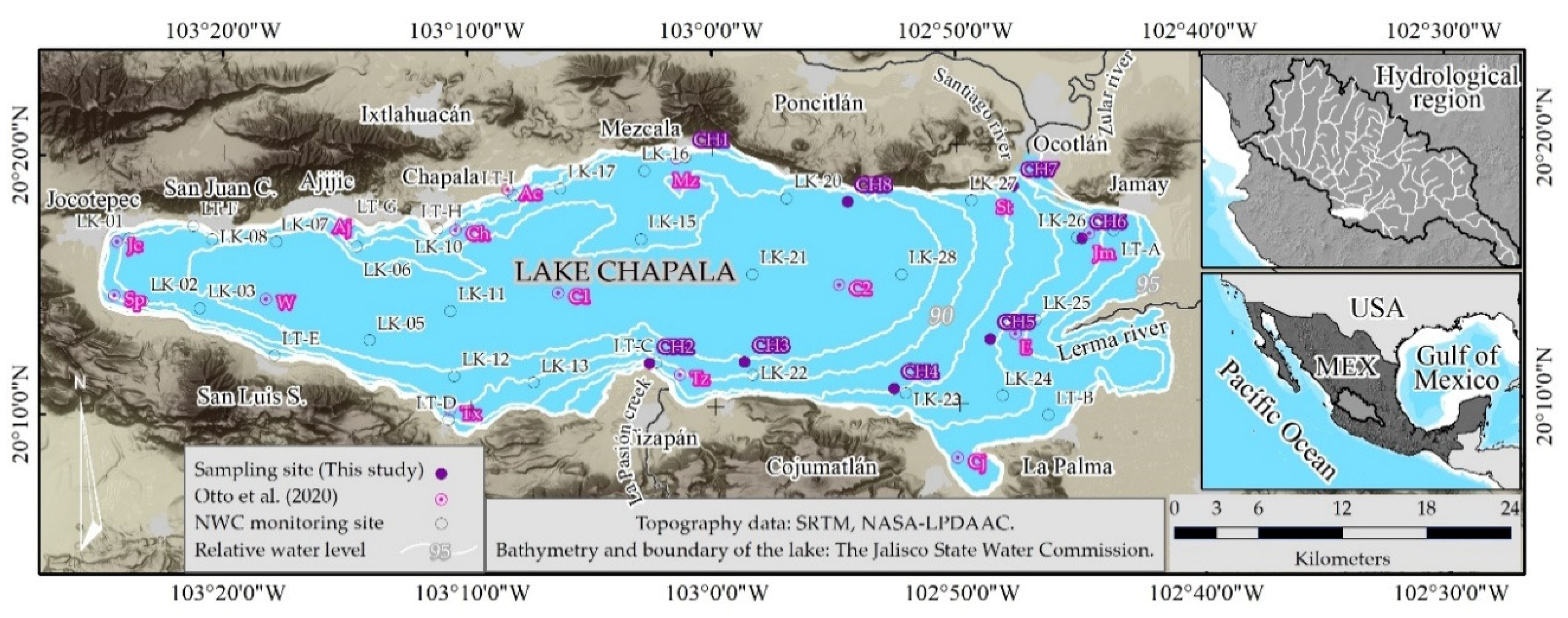
Lake Chapala, the largest lake in Mexico, spans a surface area of approximately 1100 km2, with a length of 75 km and an average width of 5.5 km (Figure 1). It is recognized as one of the largest and most shallow tropical climates [18,20]. The primary sources of water inflow are the Lerma River and La Pasión Creek, which also contribute significantly to the influx of inorganic sediments [4]. Consequently, since the late 1970s, the eastern side of the lake has exhibited the highest concentration of solids [21]. The turbidity of Lake Chapala has notably increased following a reduction in storage volume at the end of the 1970s [5]. Turbidity is predominantly influenced by suspended matter, primarily composed of clay-rich sediments, which undergo constant recirculation within the water column [4,22]. The eastern sector of the lake is particularly noteworthy due to its elevated turbidity levels. Previous research has demonstrated that this shallow water area provides favorable conditions, such as water column mixing, photic depth, and nitrogen availability as a limiting nutrient for phytoplankton photosynthesis, thereby promoting eventual growth of algae [20,23]. Additionally, significant seasonal variations in turbidity have been reported in this area, with higher turbidity during the dry season and lower turbidity during the rainy season, associated with the depth of the water column [4]. In light of these considerations and through the analysis of historical Landsat images, eight sampling sites were identified to conduct five campaigns for measuring turbidity and surface reflectance, in proximity to certain sites of the National Water Commission (NWC) in Lake Chapala (Figure 1).
The Lerma River constitutes one of the principal hydrographic basin systems in Mexico, encompassing a surface area of 47,116 km2 and exhibiting an average annual surface runoff of 4742 hm3 [24]. The river is responsible for transporting significant quantities of solids, a result of erosion processes mainly due to inadequate soil management practices [25,26]. Furthermore, the Lerma River carries pollutants from upstream areas to the lake, originating from agricultural, livestock, and industrial activities. Some pollutants remain untreated, threatening the lake’s ecosystem [27,28].

2.2. Historical Turbidity Measurements

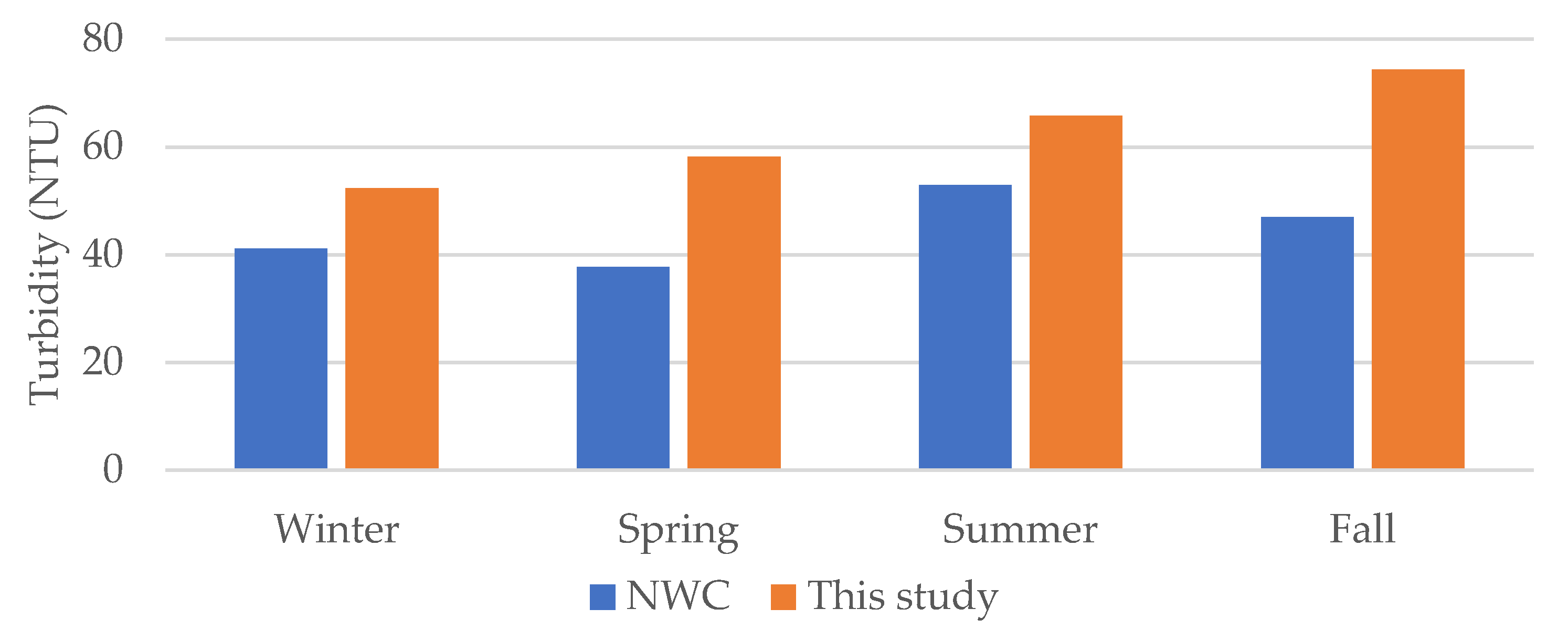
In Mexico, the NWC is responsible for overseeing the country’s water quality monitoring system. They conducted measurements at 34 sampling sites in Lake Chapala. We utilized data sources from 2000 to 2018 to calculate turbidity statistics, as well as to ascertain trends, typical behavior, and intra-annual variations for reference purposes. This dataset comprised 904 turbidity records for the specified period. From 2005 to 2018, an average of 62 measurements were recorded annually, corresponding to two samplings per site per year.

2.3. Landsat Image Processing

A collection of 41 Landsat images, encompassing six spectral bands within the visible-shortwave infrared region (VIS-SWIR2), was assembled from 22 June 2023 to 23 November 2024. This dataset was obtained from the Landsat 8 and 9 satellites (Collection 2, Level 2), which are products derived from the Land Surface Reflectance Code (LaSRC). These products incorporate implicit radiometric enhancements, atmospheric and topographic corrections, and mitigation of bidirectional effects associated with the geometric relationship between the sun and sensor angles [29,30], thereby ensuring spatial, temporal, and radiometric conformity. Such procedures provide precise measurements of surface reflectance above the Earth’s surface, thereby enhancing the consistency and comparability of images captured at different times [31].
We considered additional data concerning the pixel quality assessment (PQA) band of Landsat 8 and 9 to effectively filter artifacts from the images and isolate the affected surface. The PQA band is a derivative sub-product of the LaSRC, comprising pixel values encoded within a radiometric depth range of to 2^16, specifically digital numbers (DN) from 1 to 57,240 [32]. These values are indicative of the likelihood of pixels corresponding to artifacts, with spectral response related to snow, ice cover, clouds, cloud shadows, or water. The arrangement of these values is such that a higher digital number indicates a higher probability. We implemented a geoprocessing procedure to filter the images, thereby retaining pixels that are unaffected by cloudiness and shadows.
We utilized a conditional algorithm to classify the PQA-band from the DN values [32] to Boolean values. Specifically, we assigned a value of 1 to pixels exhibiting a low probability of cloudiness and its shadow, defined as DN ≤ 22,270 and not equal to DN = 1. Values not meeting this criterion were nullified using the following expression:
If (input1 ! = 1 and input1 <= 22,270) then (input1/input1) else null
where input1 corresponds to the PQA-band. The second step performs the reflectance calculation for the VIS-SWIR2 bands, based on the surface enabled by the previous PQA-band output that uses the following expression:
If (input1 = 1) then ((input2 * M) + A) else null
Having PQA-band as input1 and any VIS-SWIR2 band as input2. The parameters M and A represent the multiplicative scale factor (2.75 × 10⁻⁵) and additive scale factor (−0.2), respectively, for calibrating the DN to reflectance values. Furthermore, a ratio of the SWIR1 band over the BLUE band was employed to extract pixels corresponding to the water surface of Lake Chapala as follows:
If (input1/input2 < 1.0) then input3 else null
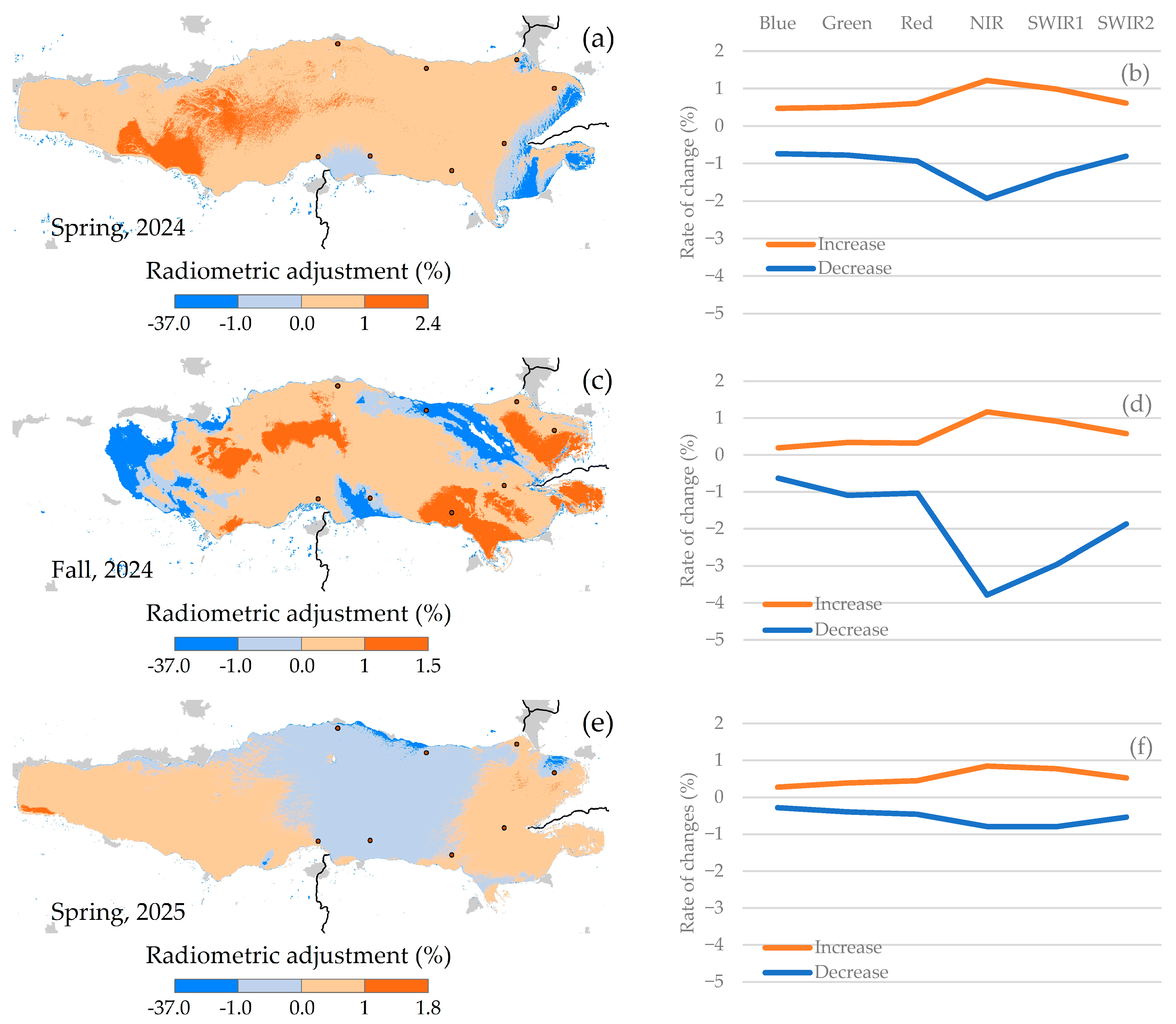
where the SWIR1 and BLUE bands correspond to input1 and input2, respectively, while input3 represents any band of the VIS-SWIR2 spectrum. This study leverages the observation that the disparity in reflectance values between these bands is usually most noticeable when examining the spectral response of water. As a result, ratios less than 1 suggest pixels associated with inland water bodies. Furthermore, the images underwent correction to mitigate the sun-glint effect, a common occurrence on water surfaces. This effect is caused by specular reflection at the air–water interface, just above the water column’s surface, and is directed towards the satellite [15]. A statistical approach (Equation (1)) was used, which originally relies on the variance and covariance (Equation (2)) of the reflectance between the VIS bands related to the near-infrared (NIR) [33].
ρ i = ρ i ( r i j ρ j ρ ¯ j )
r i j = C o v ρ i j V a r ρ j    
where:
ρ i Reflectance corrected by the sun-glint effect.
ρ i , ρ j Reflectance in any band, reflectance of the NIR band.
r i j Coefficient of covariance.
In this study, we applied the method with a slight modification by using the SWIR2 band as a reference to correct the sun-glint effect in the VIS-NIR bands, as shown in previous studies [34,35]. The use of the SWIR2 band helps in reducing the scattering light effect that might be observed in the NIR region due to the optical response of suspended matter.

2.4. Field Measurements of Reflectance and Turbidity

We conducted five campaigns to measure surface reflectance in situ at eight sampling sites on the eastern side of Lake Chapala between 2023 and 2025 (Table 1), an area characterized by the highest turbidity contrast in the lake [16]. The number of sampling campaigns and sites was determined based on available resources, the size of the lake, and the time lag between in situ measurements and the satellite pass.
The number of samples was limited; however, we conducted a comprehensive analysis of Landsat images from the last 10 years to meticulously identify optimal locations for the sampling sites. We selected sites in areas where sediment plumes are typically observed, as well as sites where such plume movement is atypical. Furthermore, historical turbidity data from monitoring sites in proximity to our sampling locations enabled us to validate these selections. Notably, our field measurements encompass 80% of the turbidity range historically recorded by the NWC.
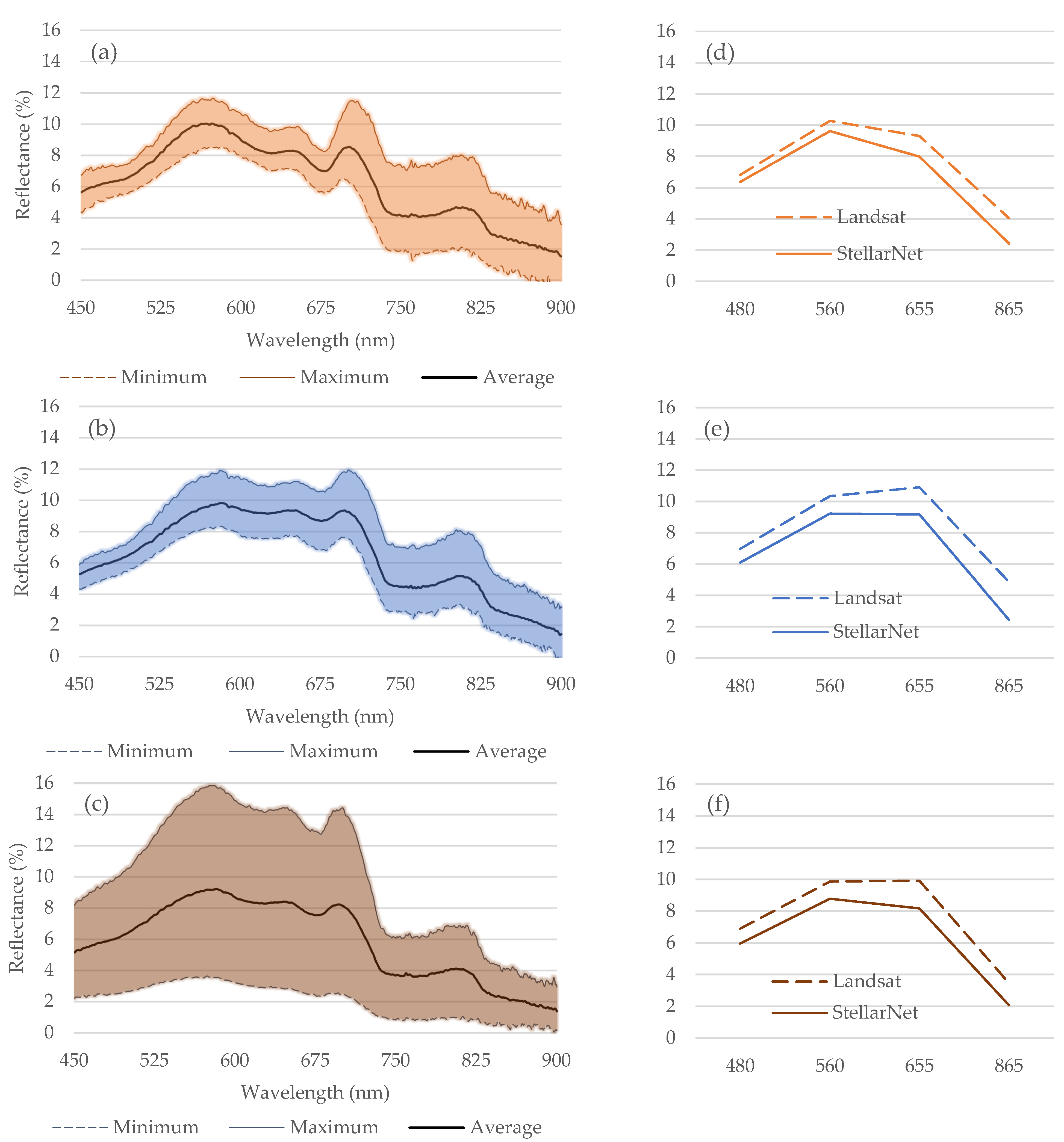
These conditions, coupled with the interest in comparing water surface reflectance from two different information sources, necessitated the scheduling of seasonal sampling. Historical turbidity data facilitated the determination of seasonal frequency, as it more accurately reflects intra-annual turbidity variation compared to monthly frequency analysis. A spectrometer (StellarNet, Black Comet SX-200, Tampa, FL, USA) with a spectral resolution of 0.5 nm was employed to capture the spectral signature of the water surface in the VIS-NIR region (450–900 nm). At each site, three measurements were conducted, with each measurement representing the average of five spectra (900 reflectance records per spectrum), resulting in 15 spectra per site and 120 spectra per campaign. We calculated the average reflectance of the VIS-NIR region, constrained to the bandwidth defined by the Landsat 8 and 9 platforms (https://www.usgs.gov/landsat-missions/landsat-9, accessed on 4 May 2025) for subsequent analysis.
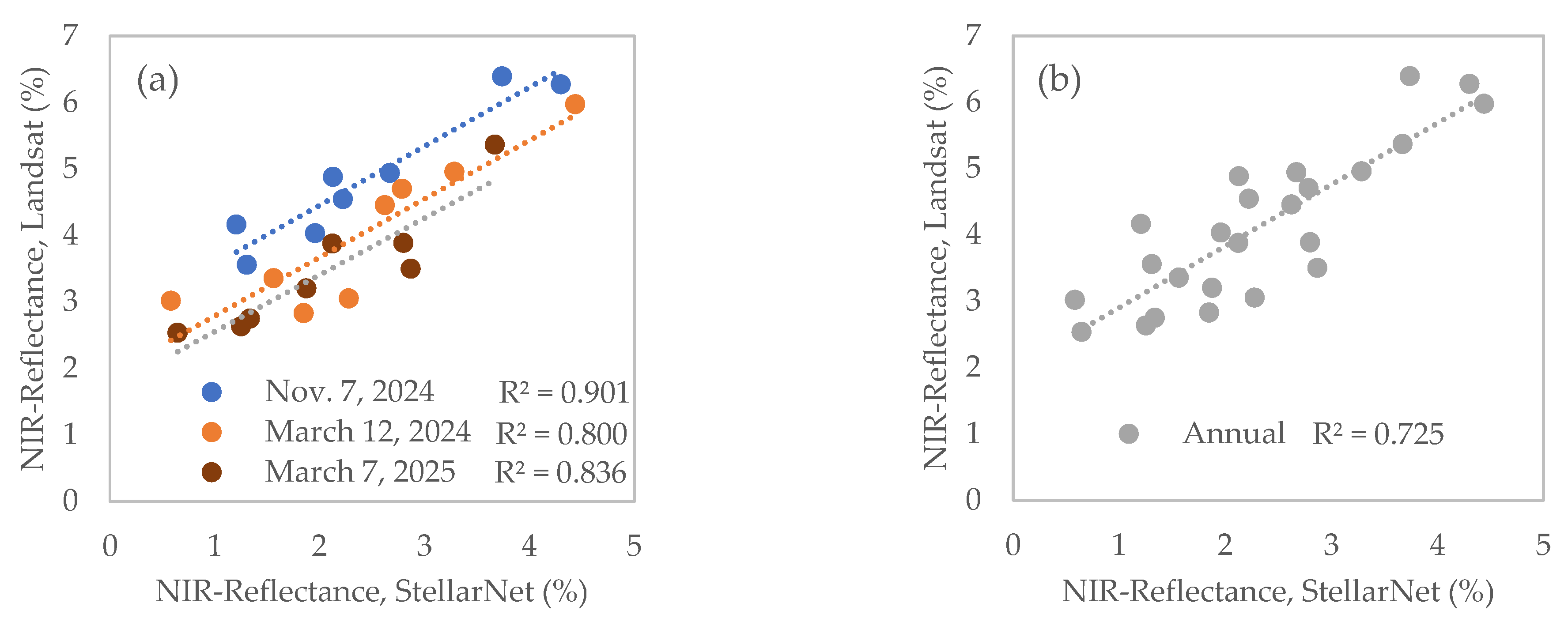
The in situ surface reflectance measurements were utilized to validate the satellite observations. However, the presence of cloudy sky conditions partially compromised the quality of satellite imagery across all campaigns. Notably, during two of the five data collection campaigns (29 November 2023 and 7 May 2024), the overcast sky resulted in a complete absence of satellite reflectance data, thereby affecting the comparative analysis between the two data sources. In the remaining three campaigns, conducted on 12 March 2024, 7 November 2024, and 7 March 2025, we calculated the average in situ surface reflectance at eight sites within a ±3-h window surrounding the Landsat satellite overpass, which is around 11:18 local time.
These samples are considered representative of the spring and fall seasons, respectively, to evaluate the model’s response within these temporal contexts. Turbidity was concurrently measured in the field at the same eight sampling sites. Turbidity was optically quantified in nephelometric turbidity units (NTU) using a Hanna portable turbidimeter HI-93703 scanner (Nusfalau, Romania), which detects light dispersion at 860 ± 10 nm, in accordance with ISO 7027-1:2016 standards. This spectral range closely aligns with the Landsat NIR spectral range (850–880 nm), providing certainty for comparative analysis between data sources, while also ensuring independence from measurements in other spectral regions and the multispectral analysis itself. Both in situ turbidity and surface reflectance were measured quasi-synchronously with the satellite overpass.

2.5. Time Series Construction and Statistical Analysis

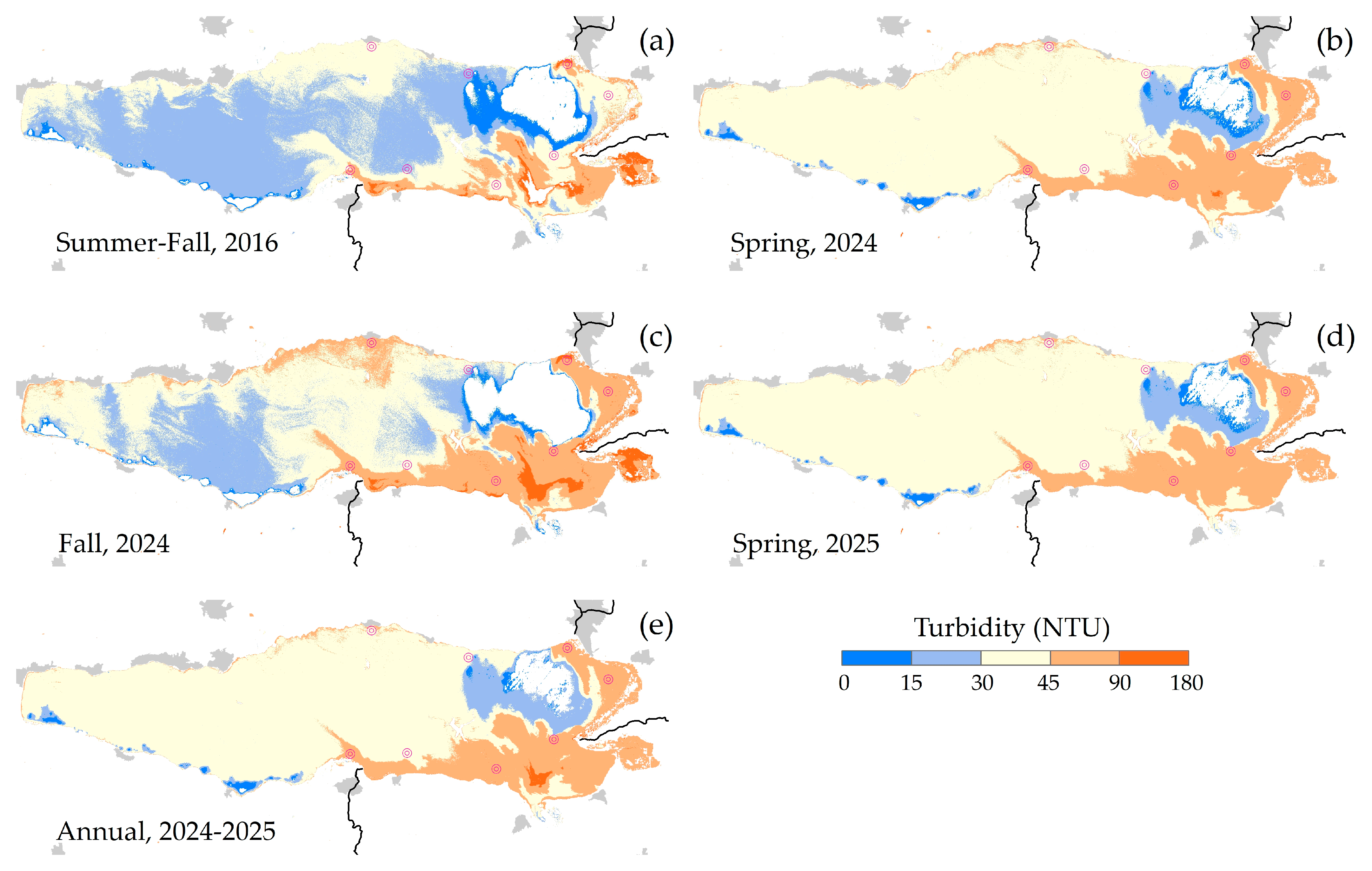
All images were integrated into a datacube to construct a time series and analyze the statistical properties of reflectance in Lake Chapala. The datacube consists of 246 bands (41 images, each consisting of six bands), partially covering the surface of Lake Chapala. The time series represents the mean reflectance value and complementary statistical parameters for each band in the datacube. This time series facilitates the identification of intra-annual variations in water reflectance between June 2023 and November 2024. The images were affected by cloud cover and their shadows, resulting in surfaces with null pixels. A sufficiency criterion of 80 percent or greater was employed to recover pixels with valid information in each band of the datacube. This criterion ensures the retention of all pixels with reflectance values in at least 196 of the 246 bands, equivalent to 33 of the 41 images. The calculation of descriptive statistics at the pixel level enabled the characterization of water reflectance behavior over time. The integration of statistical parameters (average, minimum, maximum, standard deviation, range, and count) per pixel and band facilitated the identification of spatial contrasts in the typical spectral response of water in Lake Chapala, particularly concerning the NIR surface reflectance.

2.6. Spatial Prediction Model

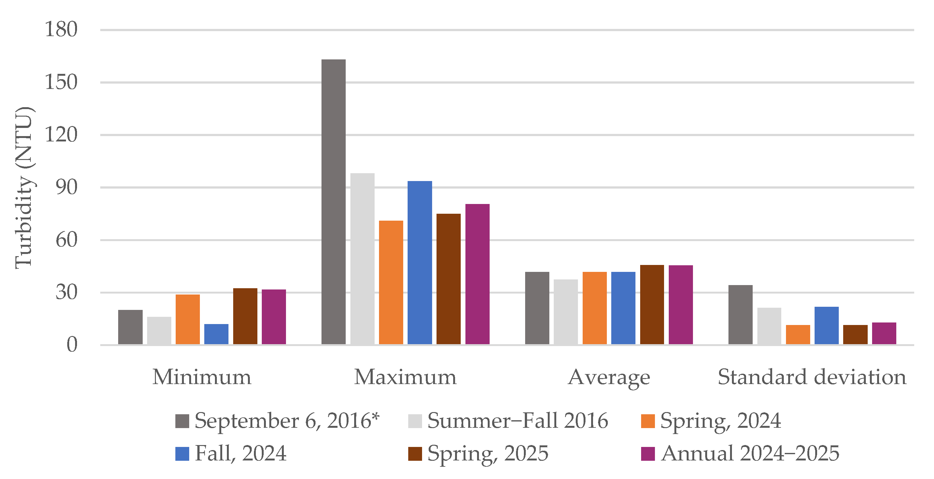
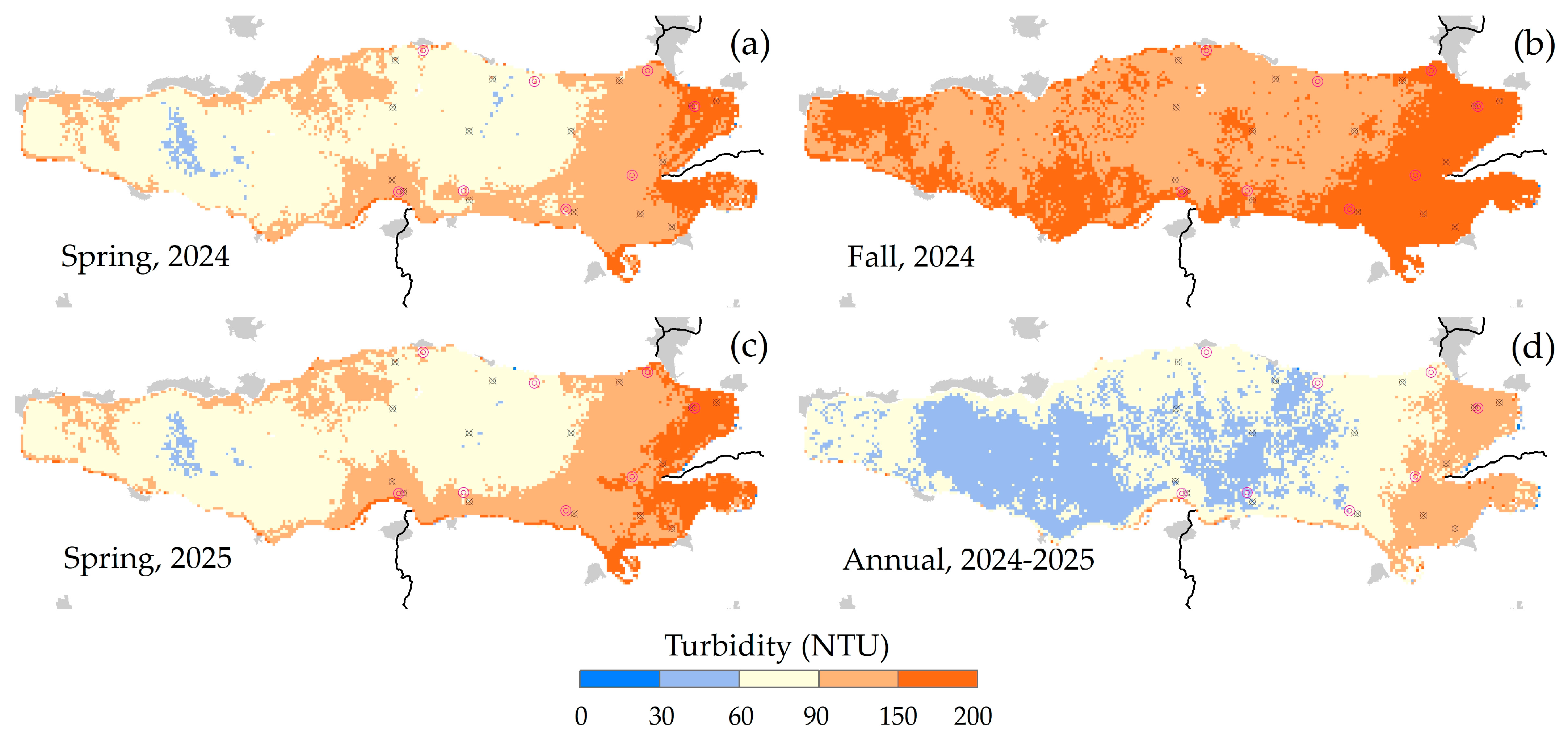
The model’s construction was undertaken in three distinct phases. Initially, satellite surface reflectance was validated through field measurements. This comparative analysis between data sources enabled the evaluation of the reliability of satellite data via linear correlations for the dates of 12 March 2024, 7 November 2024, and 7 March 2025. In the subsequent phase, nonlinear correlations between in situ turbidity and satellite NIR surface reflectance measurements facilitated the development of empirical turbidity models to estimate the magnitude and spatial distribution of turbidity in Lake Chapala. Quasi-synchronous data from the three campaigns were utilized to construct spatial prediction models. Two second-degree polynomial functions were formulated to estimate turbidity based on satellite surface reflectance at the eight sampling sites for each campaign. These models were applied to the corresponding Landsat imagery to estimate turbidity in Lake Chapala. The reliability of each turbidity model was assessed using linear correlations with field observations at the eight sampling sites. Furthermore, the three campaigns were integrated into a single series to establish a standardized annual model (2024–2025). In the final phase, the response of the turbidity prediction models was evaluated for spring (12 March 2024 and 7 March 2025), fall (7 November 2024), and the annual cycle. The statistical validation was conducted by applying the models to a specific case evaluated in 2016 [16]. The response of each model was assessed through linear correlations between the turbidity estimated by the models and the turbidity measured in that study at the 15 sampling sites. Validation was also performed using the historical WNC data measured at 34 sampling sites. The four models (Equations (3)–(6)) were applied to the NIR band for all 41 Landsat images. A turbidity time series derived from these images was integrated for each model to calculate the pixel-by-pixel descriptive statistics and map the estimated turbidity across the entire lake, as detailed in Section 2.5.

3. Results

3.1. Turbidity

The statistical analysis of 904 historical records from the period 2000–2018 reveals that turbidity exhibits a non-normal distribution characterized by a right-skewed tail, with values ranging from 2 to 190 NTU and an average turbidity of 31.5 ± 23.5 NTU. Notably, significant differences in turbidity are observed when the lake is divided into two regions: west and east (Figure 2). The western region typically displays low turbidity values ranging from 2 to 54 NTU, with an average of 26.9 NTU, and atypical values reaching up to 75 NTU (Figure 2a). In contrast, the eastern region typically exhibits values ranging from 2 to 87 NTU, with an average of 39.8 NTU, and atypical values ranging up to 124 NTU (Figure 2b). An analysis of variance (ANOVA) between the western and eastern regions revealed significant differences in the median turbidity (p-value = 0.0000003) at a 95% confidence level, which is the standard for all statistical tests in this study. Given that the eastern region demonstrates the greatest spatial variation, including the lowest turbidity values observed in the western lake, our research focused on this area for model development and evaluation.
Conversely, statistical analysis of in situ turbidity data collected at eight sites across five sampling campaigns reveals that this data also exhibits a non-normal distribution, similar to the historical data. Significant differences were identified between the sites, while similarities were observed among groups based on the survey date (Table 2). Specifically, the ANOVA based on multiple sample comparisons and the Kruskal–Wallis test indicated a significant difference between the medians of the eight sites (p-value of 0.01462). The analysis highlights elevated turbidity levels at sites on the southeastern side of the lake (CH4 to CH7), with values surpassing the grand average (total values in Table 2(a)) compared to turbidity measured towards the central lake. These findings suggest that this lake area is characterized by the highest turbidity. The analysis also revealed some similarities in turbidity medians between the sites. Notably, turbidity at sites CH2 and CH7 was significant due to the site locations corresponding to the La Pasion Creek and Lake Chapala outlets. Temporal transition is another significant factor influencing turbidity in Lake Chapala, as previously documented in the literature [4]. Statistics (Table 2(b)) and ANOVA among seasons based on the Kruskal–Wallis test demonstrated that there were no significant differences in turbidity between dates (p-value = 0.39761), despite seasonal changes involving variations in the supply of water and sediment to the lake or lake level (water volume). All the mean turbidities by season formed a homogeneous group with low variation.
Our measurements were strategically scheduled to obtain representative data for each season, aligning with the Landsat satellite flight schedule and prevailing meteorological conditions. We deliberately avoided scheduling studies during or near the summer months due to the high likelihood of cloudy skies. In practice, adjustments to the measurement schedule were necessitated by meteorological complications, which did not always ensure clear sky conditions for all sampling campaigns. Nonetheless, our measurements effectively represented all four seasons, particularly in light of the altered climate regime resulting from the drought conditions prevalent in western Mexico. Consequently, we conducted a comparative analysis between our data sources and official NWC data to verify the consistency of these measurements, focusing on seasonal variations in turbidity during the period 2000–2018 (Figure 3).
The statistical analysis of the four NWC seasons, along with the five datasets from this study (according to each season), revealed a normal distribution. The results of the multiple comparison ANOVA and the Kruskal–Wallis test indicated no significant differences among the eight means (p = 0.10544). Notably, the mean turbidity for the fall season in this study was marginally higher than the other means. The turbidity recorded on 7 November 2024 was particularly notable, yet it remained within the typical range observed from 2000 to 2018.

3.2. Radiometric Improvements

The spatial delimitation procedures, which involve radiometric calibration (conversion from digital numbers to surface reflectance), artifact subtraction utilizing PQA-band properties, and water masking through a band ratio, enabled us to isolate the water surface reflectance of Lake Chapala, thereby excluding non-water surfaces. Within these effective areas, the radiometric adjustment through sun-glint effect correction enhanced the images, facilitating a more accurate assessment of turbidity. We evaluated the images employed to develop the spatial turbidity prediction model. Lyzenga’s method, which estimates a rescaling coefficient based on the covariance of the SWIR2 band and each VIS-NIR band, requires a radiometric adjustment for all pixels in the effective scene, thereby balancing the brightness and darkness areas of the lake. We calculated the difference in surface reflectance in pixels before and after sun-glint correction to estimate the rate of change. The statistics of the minimum and maximum values of surface reflectance, encompassing 99% of the pixels in each image, indicated that the rate of change per band in the VIR region was predominantly within or around ±1%. In contrast, the rate of change in the NIR ranged from −1.93% to 1.22% in spring, and from −3.79% to 1.17% in the fall season (Figure 4a,c,e). In particular, we illustrate the radiometric adjustment of the NIR band to exemplify the spatial distribution of the rate of change estimated in such images (Figure 4b,d,f). The maps depict the spatial distribution and magnitude of these rates, delineating the regions where Lyzenga’s rescaling coefficient resulted in the darkening of bright areas (thereby reducing water surface reflectance) as indicated by negative values or blue areas, and conversely, where it brightened areas, as shown by positive values or orange areas.

3.3. Validation of the Satellite Surface Reflectance

Under clear sky conditions, the analysis of water surface reflectance revealed that the complete spectrum of in situ water demonstrated consistent patterns across different seasons, with minor variations in magnitude observed within the 570–700 nm range (Figure 5a–c). However, when examining the surface reflectance within the regions defined by the Landsat 8–9 platforms (https://www.usgs.gov/landsat-missions/landsat-9, accessed on 4 May 2025), the analysis of variance for these non-normal distributions, through the Mann–Whitney test, indicated no significant differences in the medians (p-value = 0.31698) of in situ measured surface reflectance between seasons (Figure 5d–f). Furthermore, the correlation analysis of the water spectral pattern between the spring and fall seasons demonstrated a high degree of similarity (R2 = 0.95), with no significant differences (p ≈ 0.00001).
We estimated the in situ average surface reflectance, confined to the VIS-NIR region, as established on the Landsat 8 and 9 platforms for analysis (Figure 5d–f). Under these conditions and considering that information is limited to the specific conditions of 2024, an ANOVA based on multiple comparisons using the Kruskal–Wallis test revealed no significant differences between the measurement sources (Landsat vs. StellarNet) or between seasons (spring vs. fall) (p-value = 0.84284). These findings tell us that satellite data possess a high level of reliability in predicting spatial turbidity. Additionally, we developed a combined model that considers data from both seasons as the average model for the annual cycle. In this context, the correlation analysis between the VIS-NIR spectral signals of both sources indicates that the satellite data effectively explains the variation in the field data, even when the annual model is applied (Table 3).
In this study, the near-infrared (NIR) water surface reflectance was evaluated by comparing satellite data with in situ measurements on a site-specific basis. The correlation between these data sources was notably strong during both the spring (12 March 2024 and 7 March 2025) and fall (7 November 2024) seasons, with R-values of 0.894 and 0.949, respectively. These correlations suggest that satellite reflectance accounts for 80.0% to 90.1% of the variability observed in the in situ reflectance (p-value < 0.05) (Figure 6a). Furthermore, when the data were analyzed as a single combined series, a strong correlation was observed (R = 0.857), with satellite data explaining 73.5% of the variability in the in situ measurements (p-Value = 0.00001) (Figure 6b).
The findings substantiate and validate the use of satellite-based modeling for monitoring water quality parameters, such as turbidity. The model exhibited satisfactory predictive accuracy; however, it is important to note that error dispersion varied seasonally. The standard error and mean absolute error ranged from approximately 6 to 30 NTU, depending on the campaign, with lower errors observed during the spring season and increased variability during the fall.

3.4. Modeling the Spatial Turbidity

The Landsat NIR-reflectance, validated at the eight sampling sites (Figure 6), was correlated with the corresponding turbidity measurements to develop predictive models. The nonlinear relationships between the variables were explained by a second-order polynomial function to forecast spatial turbidity during the spring and fall seasons (Equations (3)–(5), respectively). This model was the most effective in simply explaining the behavior of turbidity in Lake Chapala. Additionally, the integration of data from both seasons enabled the development of a model for the annual cycle (Equation (6)).
T u r b i d i t y N T U = 3.0 × 10 5 +   3.0 × 10 5 2 4 ( 0.038 ) ( 1.677 ρ N I R ) 2 ( 0.038 )           S p r i n g   2024  
T u r b i d i t y N T U = 3.0 × 10 5 +   3.0 × 10 5 2 4 ( 0.011 ) ( 3.655 ρ N I R ) 2 ( 0.011 )           F a l l ,   2024
T u r b i d i t y N T U = 1.0 × 10 5 +   1.0 × 10 5 2 4 ( 0.035 ) ( 1.654 ρ N I R ) 2 ( 0.035 )           S p r i n g   2025
T u r b i d i t y N T U = 1.0 × 10 4 +   1.0 × 10 4 2 4 ( 0.053 ) ( 1.227 ρ N I R ) 2 ( 0.053 )           A n n u a l
The coefficients used in these equations are the result of the polynomial fit of each model (Table 4). The dependent variable (in this case, NIR reflectance in percentage terms) was solved using the quadratic equation model.
The spring and fall models utilizing Landsat imagery elucidate the spatial distribution of turbidity for each season between 2024 and 2025. In these instances, the modeling underscores significant contrasts between the eastern lake and the remaining surface area (Figure 7a–c).
The turbidity estimated using Equations (3)–(6) exhibits strong correlations with measurements obtained from the eight sampling sites, which served as the basis for model development. Model evaluation, using statistical parameters derived from both model construction (Table 5(a)) and evaluation (Table 5(b)), indicated that the model performed effectively, as evidenced by a Spearman coefficient (R > 0.9). The turbidity estimates accounted for 81–96% of the variability (R2) in turbidity observations in the eastern region of Lake Chapala (Table 5(b)). Notably, the spring and annual models demonstrated the best fit, characterized by the lowest Standard Error (SE) and Mean Absolute Error (MAE) values. These findings suggest that both models are valuable tools for predicting turbidity in Lake Chapala.
It is crucial to acknowledge that the number of sampling sites is small, but also that the relationship between the rate of change in surface reflectance and turbidity is quite asymmetric. We performed a spatial autocorrelation analysis of the turbidity estimates modeled by the four models applied to the 41 satellite images. Overall, the Anselin–Moran index, based on statistical metrics such as z-scores and p-values, showed that nearly 70% of the data are “clustered” as low or high turbidity values, and 31% followed a spatial pattern of apparent randomness. Finally, a very small data set, scattered mainly along the lakeshore, was classified as outliers. These results do not justify the high correlation coefficients and minimal error estimates of the turbidity prediction models. However, these give us confidence to suggest that the selection of sampling sites based on the historical record of the Landsat collection and the national water quality monitoring system in Mexico allowed us to obtain representative samples that validate the predictive capacity of the empirical models.
In this sense, we conduct a global sensitivity analysis of the models to elucidate the degree of asymmetry directly associated with the stochastic behavior of the water currents located on the western side of the lake. This analysis was grounded in statistical parameters derived from each data subset, including in situ turbidity, satellite surface reflectance, and estimated turbidity. Despite the nonlinear relationship between turbidity and NIR surface reflectance, this analysis reveals that the models exhibit considerable sensitivity and are strongly dependent on the rate of change of surface reflectance. A small change in the magnitude of surface reflectance translates into significant changes in the rate of change of turbidity. This strong dependence has important implications for the analysis of satellite images, as the effects of atmospheric, meteorological, or light phenomena produce important deviations between actual reflectance and satellite capture. Concurrently, these phenomena can induce deviations from the in situ turbidity, leading to increased model uncertainty. The quality of Landsat imagery (Collection 2, Level 2) effectively mitigates the interference caused by most of these physical phenomena; however, the sun glint effect remains unresolved. It is noteworthy that any radiometric geoprocessing technique employed to isolate the spectral response of water can ascertain the coefficients of the polynomial function that elucidates the relationship between the two variables. Since correcting for sun glint effects implies substantial improvements in the radiometric quality of satellite data [15], we adopted the methodological proposal by Lyzenga et al. [33] to systematically reduce the brightness contrast effect inherent to the surface dynamics of the water body. In the image after the glint-effect correction, the difference between the turbidity measured and estimated regarding the ratio over the surface reflectance (T/SR) is lower than the pre-corrections (Table 6).
These reductions point out that such a correction procedure enhanced the model predictions, at least for the spring models. Conversely, the adjustment for the fall season model demonstrates that the correction for the sun glint effect results in an overestimation of turbidity values, thereby increasing the difference between the T/SR values of the measured and estimated turbidity.

3.5. Statistical Validation

3.5.1. Specific Case: In Situ Data from 2016

We analyzed the responses of the three models to evaluate their accuracy in spatial prediction, as outlined in Equations (3)–(6), across two temporal scales: a specific date and historical records. For the first scale, the models were applied to a single date (image), and their outputs were compared with the response of another model documented in a previous study [16] to estimate turbidity in Lake Chapala. The turbidity estimates from the three models were approximately twice the turbidity measured at the 15 sampling sites in 2016. This discrepancy is attributed to the number of sites used to build these three models, which was lower than that of 2016. There are seven sites in 2016 that did not record measurements in 2023–2024, these sites were located in the western sector of the lake, where turbidity is much lower and exhibits less spatial and temporal variability.
A spatial comparison between the turbidity measured in 2016 and that estimated by each model reveals that the horizontal rate of change is virtually the same, despite having a mean deviation twice that of the 2016 measurements. This spatial overlap indicates that the difference between the two data sources lies in sample size. More importantly, it validates the representativeness of the polynomial regression model based on the eight sampling sites in the eastern sector of the lake, akin to the regression used by Otto et al. [16]. In this context, we calculated a rescaling factor for the estimated turbidity to demonstrate the degree of deviation of each model for instantaneous events (Table 7).
The rescaling factor functioned as a systematic bias correction, calculated as the mean value of the discrepancies between the in situ turbidity measurements (6 September 2016) and the modeled turbidity across the 15 sites, their results range between 0.445 and 0.505. This rescaling also facilitated the adjustment of the ordinal values of the modeled turbidity using the in situ measurements (Figure 8).
The statistical analysis reveals that the spring and annual models exhibit a tendency to overestimate the minimum turbidity while underestimating the maximum turbidity observed in 2016 (Figure 9). However, the most noteworthy finding is that these models produce average values that are closely aligned with the 2016 measurements, demonstrating a reduced deviation.
Each model underwent statistical validation through a linear correlation analysis between the turbidity measured at the 15 sampling sites on 6 September 2016 and the turbidity estimated by the five models (Table 8). The annual (2024–2025) model demonstrated the best fit among the models from this study, exhibiting a strong correlation that accounted for approximately 70% of the variability in the field-measured turbidity on 6 September 2016, and also produced the lowest SE and MAE. This outcome is comparable to the summer–fall model of 2016.
Their predictive spatial capacity was comparable to the model proposed by Otto et al. [16]. The rescaling factors employed to adjust the estimated turbidities in this specific case effectively reduced the prediction error without affecting the correlation coefficients or the level of statistical significance, which remained consistent with their previously calculated values. In this instance, we observed relatively high average turbidity measurements per campaign compared to the 2016 average, albeit with narrower ranges. These statistical characteristics of the data used to construct the model account for the overestimation of the observed turbidity and justify the application of such rescaling factors.

3.5.2. Historical Monitoring Data (2000–2018)

Statistical validation utilizing historical data constitutes an additional approach for evaluating satellite-derived turbidity based on the output response of the four models. A turbidity datacube was constructed for each model to delineate its temporal pattern throughout the entire annual cycle from 2023 to 2024. Each pixel within the cube represents a time series consisting of 41 records, corresponding to the total number of Landsat images. The mean values for each pixel were employed to characterize the typical turbidity in Lake Chapala, as derived from the spring, fall, and annual models (Figure 10).
On the other side, the average turbidity records from 2000 to 2018, collected from 34 monitoring sites by the NWC, have served as references. These data were categorized both annually and seasonally to examine intra-annual variations. Specifically, the analysis focused on the average turbidity corresponding to the geographical location of each site. The mean turbidity estimated through the models (Figure 10) was compared with the mean seasonal and annual turbidity derived from historical data. It was observed that the spring models both estimated an average turbidity 2.75 times (2.49–2.97) greater than the typical seasonal turbidity. The fall model indicated a turbidity 4.14 times (3.77–4.50) higher than the typical value. Among the four models, the annual model exhibited the lowest proportion, with turbidity 1.99 times (1.79–2.15) the typical seasonal value. In this context, the rescaling factors applied to adjust the turbidity estimates did not enhance the predictive accuracy of the models but rather introduced inaccuracies in their output. Consequently, a validation was conducted using the output responses derived from Equations (3)–(6) without correction factors.
We carried out linear correlations in the 34 sites to the whole lake and in the 15 sites to the eastern side of the lake. The comparison between them showed that all turbidity models have good correlation in the case of the eastern side of the lake (Table 9), just the area where we take information for the model construction. The spring and annual models showed better adjustment in comparison with the fall model, which explained the mean seasonal turbidity for the typical turbidity measured between the years of 2000 and 2018. The analysis in the whole lake showed that only the spring (2025) model predicted the seasonal turbidity for almost the entire season with a certainty level of 64 to 87%. The remaining models presented some difficulty in characterizing the typical turbidity in such a period (Table 9(a)). While on the eastern side of the lake, the spring and annual models explained between 67 and 92% of the typical turbidity, whose uncertainty without considering the annual turbidity was from greatest to least in the following order: spring > winter > fall (Table 9(b)). The data indicate the robust performance of the models concerning the typical turbidity conditions observed during the period 2000–2018. The predictive capabilities of both the spring and annual models are noteworthy, showing acceptable accuracy in explaining the annual mean turbidity and typical turbidity by season on the eastern side of the lake. The annual model accounts for the typical turbidity by season, overestimating, on average, twice the measured values by site. However, site-by-site analysis reveals that the discrepancies between the modeled and observed turbidity are uniform along the lake and across the seasons.

4. Discussion

4.1. Importance of the Field Spectral Validation

Remote sensing research in aquatic environments constitutes a critical resource for the effective implementation of management programs and the provision of decision-making support aimed at preserving water quality and ecosystem health. Consequently, a certainty factor associated with the interpretation of satellite data is essential. Currently, the optical response of materials or their components can be documented in comprehensive spectral libraries, which frequently serve as references for validating satellite data. In many instances, this is advantageous because the optical properties of objects or surfaces exhibit minimal variation over time or across extensive areas, such as the mineralogical composition of a rock. Conversely, in other instances, they may prove inadequate due to the dynamic behavior of objects or surfaces, such as a body of water, which is highly variable. Unlike previous studies conducted in Lake Chapala and adjacent water bodies, our research incorporates quasi-synchronous field surface reflectance measurements as a fundamental element of satellite data validation, a practice seldom employed in this type of research (Figure 5). Through these measurements, the Pearson coefficient was determined to exceed 0.95 in the VIS-NIR reflectance between in situ data and Landsat images. Specifically, Landsat NIR reflectance correlates with field measurements ranging from 0.89 to 0.95 (Figure 6), thereby providing a high degree of certainty to satellite observations.
This observed level of correlation is considered acceptable and instills confidence in the satellite data. This finding underscores the high quality of Landsat imagery, as it effectively mitigates the effects of various factors that compromise its quality compared to early Landsat products (e.g., Standard Level 1 products) or other satellite datasets (Spot) used for assessing water quality in Lake Chapala. These factors encompass topographic, atmospheric, and bidirectional effects associated with the geometric relationships in the direction of light from the sun, its path through the atmosphere, and its interaction with satellite sensors [29,30]. Furthermore, direct validation assured the turbidity prediction model, demonstrating acceptable performance despite being developed through an empirical modeling approach with a limited sample size (Table 5(a)). An initial evaluation of the performance of the Landsat surface reflectance-based models revealed that they could account for at least 81% of the variation in field-measured turbidity for the dates on which the models were constructed (Table 5(b)). The differences in estimation error across seasons suggest the presence of both random and seasonally dependent error components, potentially influenced by hydrodynamic conditions and meteorological variability. Although no significant indication of systematic bias was identified in the residual distribution, it is advisable for future research to conduct a comprehensive residual analysis and estimate confidence intervals to more accurately characterize the model’s predictive uncertainty.

4.2. Radiometric Corrections: Enhancing Image Quality

The Landsat Collection 2 and Level 2 products include the PQA-band, which significantly enhances the delineation of water surface pixels affected by clouds and their shadows. This band, in conjunction with the water mask, facilitates the exclusion of such areas from spatial analysis. The removal of these pixels also mitigates noise caused by the brightness of clouds and the darkness of their shadows, thereby improving the spectral processing for sun-glint effect correction. The method proposed by Lyzenga et al. [33] redistributes the histogram of surface reflectance based on the brightest and darkest pixels within the entire scene or effective area. The PQA-band specifically targets the response of water surface reflectance. Consequently, the sun-glint effect correction addresses the brightness resulting from specular reflection on calm water surfaces, which are prevalent in certain areas of Lake Chapala due to the absence of wind around noon, as well as the scattered light from whitecaps associated with waves in other areas of the lake, and the darkness of shallow water. This method induces a redistribution of the histogram, balancing water surface reflectance based on the brightest and darkest pixels. Such redistribution minimally affects the radiometric response of each pixel, with variations of ±1% in the VIS region and −3.78 to 1.22% in the NIR region (Figure 4), compared to other methods such as those by Goodman et al. [36] or Kutser et al. [37] in Kay et al. [15]. Areas where water surface reflectance was adjusted by up to −30% typically exhibited low values, where any change could be magnified in relative terms. Specific records from sampling sites indicated that Lyzenga’s method adjusted the Landsat surface reflectance to more closely align with field measurements (Figure 5), confirming that this adjustment enhanced the quality of the Landsat images.

4.3. Model Performance in the Context of the Machine Learning Rise

Since 2006, there has been a significant diversification in methodologies for estimating water quality using satellite imagery, shifting from a predominant reliance on empirical and semi-analytical models to an increased utilization of machine learning and mixed models [9]. Machine learning has emerged as a principal methodological approach in this domain. The predictive capabilities of various satellite-based machine learning models have been extensively validated in studies examining the optical properties of inland water bodies. These models generally yield acceptable results, ranging from those that overfit the variable’s behavior [9] to those with constrained predictive capacity [10,38]. We conducted a literature review focusing on research concerning the remote sensing of Mexican inland waters, employing machine learning and satellite data, to elucidate the disparities in predictive performance among these models. Four studies have documented the measurement of Turbidity, Chlorophyll-a (Chl-a), Total Suspended Solids (TSS), and Total Suspended Matter (TSM) in the waters of eight lakes or reservoirs, utilizing 11 machine learning models derived from six distinct data sources [13,14,39,40]. The findings of these investigations underscore the efficacy of the Extreme Learning Machine (ELM) and Linear Regression (LR) models, which achieved the highest prediction accuracy for turbidity by the lake, ranging from 67% to 91%, while the LR and Multiple Linear Regression (MLR) models demonstrated superior predictive accuracy, ranging from 76% to 98%, for the other three parameters (Table 10).
In the context of Lake Chapala, the most effective models, namely ELM and LR, exhibited limited capability in predicting turbidity, regardless of the satellite data source employed. This level of accuracy is intrinsically linked to the fact that these models utilized 10–13 images from three satellite platforms and data from 47–154 sampling sites (spanning 2012 to 2018), with turbidity measurements obtained from the NWC within a ±3-day window of the satellite pass. Remote sensing in Lake Chapala presents particular challenges due to its dynamic nature, which is significantly influenced by its size, shape, depth gradient, surrounding morphological features, variations in effluent volume, and the impact of variables such as temperature and wind speed. Despite these complexities, the performance of any empirical or semi-empirical model, including machine learning models, is subject to temporal lags, a common characteristic in research employing this methodological approach. The temporal approximation of days substantially impairs the efficacy of any model, thereby affecting the precision of its predictive capability when attempting to correlate reflectance with optical parameters, such as turbidity. Nevertheless, the application of empirical and semi-analytical models remains prevalent [9].
The utilization of empirical models is subject to scrutiny due to their methodological simplicity and the significant limitations arising from their reliance on the specific range of values employed in developing models for particular case studies. Furthermore, while satellite imagery is frequently presumed to be of high quality, and recent satellite products have shown considerable improvement, the remote sensing of water bodies encompasses aspects that require further attention. Some research studies have made such assumptions, employing satellite imagery for water quality analysis without adequately assessing data quality or, more concerningly, without implementing appropriate radiometric corrections to mitigate the uncertainty associated with radiometric artifacts. This is particularly evident when the methodological framework lacks detailed processing descriptions.
The application of these models can substantially contribute to the scientific resolution of specific issues; however, several factors warrant consideration. We employ excellent-quality Landsat 8 and 9 Collection 2 Level 2 products, which incorporate an intrinsic correction process that refines the electromagnetic signals of the objects and landforms to determine their surface reflectance accurately. Utilizing this high-quality data, we initially conducted additional processing to exclude pixels affected by clouds and their shadows, delineate the water body, and correct for the sun-glint effect. Subsequently, we assessed image quality by comparing quasi-synchronous surface reflectance measurements obtained in the field with those from the satellite’s passage, thereby verifying the quality of the satellite data. These two essential steps substantially enhance remote sensing analysis and provide increased confidence in the model responses derived from this information. The polynomial function employed here does not explain the physical behavior of the turbidity. However, our investigation based on the Landsat 8–9 sensor system indicates that turbidity (at least in Lake Chapala) exhibits such a nonlinear relationship with respect to the proportion of reflected energy. Furthermore, these empirical models are based on single-band radiometric analysis of the NIR region of the Landsat satellite, which provides a significant advantage in assessing turbidity within a spectral window (850–880 nm) that closely aligns with the optical methods employed by field or laboratory instruments (860 ± 10 nm). This analytical approach reinforced the efficacy of these empirical models. Since the eastern part of the lake exhibits all possible turbidity conditions that could occur in virtually the entire lake, we are confident that model predictions based solely on information from a few, but highly selective, sites in the eastern part of the lake are capable of estimating turbidity throughout the entire lake.
Notably, the composite (annual) model exhibited a remarkable response, with model evaluation indicating a strong coefficient of determination in explaining the spatial variation in turbidity during both the spring and fall seasons (at least R2 = 0.85), coupled with a low error (Figure 7 and Table 5). The statistical validation for a single date (one image), the model effectively accounted for the turbidity measured on 6 September 2016 (R2 = 0.69), with an error even lower than that of the model quasi-synchronously calibrated with turbidity measured on the same day (Figure 8 and Table 8). Furthermore, the statistical validation of the model, applying the annual model to 41 images between 2023 and 2024, and validation with historical turbidity data from 2000 to 2018, illustrates the typical magnitude of turbidity and its spatial distribution along the lake (Figure 10). The model’s accuracy in explaining variations in the mean annual turbidity across the lake or in the eastern sector is commendable (R2 = 0.75 and 0.78, respectively). This accuracy ranges from worse–moderate (R2 = 0.53 to 0.57) for summer, fall, and winter, to good during spring (R2 = 0.81 to 0.92). This also indicates that, despite seasonal turbidity variations, the model possesses an acceptable predictive capacity for typical seasonal turbidity behavior (Table 9).
The predictive capability of the annual model is comparable to that of other empirical models [8]. However, our study offers the advantage of utilizing a data source with better quality control. Additionally, we document enhancements in radiometric data processing, which are validated through ground-level surface reflectance measurements. This model also aligns with the predictive accuracy of machine learning-based models applied to Lake Chapala and other aquatic bodies within the east–west volcanic region of central Mexico, situated between 18°24′N and 20°25′N [13,14,39,40]. In summary, our methodological approach extends beyond establishing a mere correlation between the spectral response of water and turbidity. We propose a framework that underscores the need for satellite data processing, aims to reduce the uncertainty associated with the temporal lag of satellite data, and validates satellite data through quasi-synchronous measurements.

4.4. Environmental Implications

Lake Chapala is characterized by its dynamic internal currents and notable wave activity. Filonov and Tereshchenko [18] analyze the thermal regime and internal circulation of Lake Chapala, reporting significant surface temperature variations, particularly in the eastern part of the lake, where differences of up to 3 °C were recorded over distances of 100–300 m. These variations are associated with the formation of thermal lenses and internal solitary waves, which are generated by the displacement of warm water from the shallow eastern part toward the lake’s center, driven by the diurnal breeze. The authors also identified a cyclonic circulation in the north of the lake and an anticyclonic circulation in the southern part, influenced by weak easterly winds. Additionally, Langmuir-type circulation systems were observed to contribute to the vertical and horizontal mixing of the water. The findings underscore the importance of the morning breeze in the lake’s mixing processes and its impact on thermal distribution and internal dynamics. Specifically, Filonov [19] emphasizes that the lake breeze circulation, driven by the daily temperature cycle, plays a crucial role in the lake’s dynamics, while also increasing evaporation during the day. The effect of the morning breeze, the thermal regime, and the internal circulation of the lake are capable of producing currents with average velocities ranging from 2 to 30 cm s−1, driven by winds of 5–8 m s−1, displacing water masses over several meters or even exceeding 1 km per hour [18,19,41]. These currents result in temporal discrepancies between satellite and in situ measurements, thereby introducing uncertainties into models [16]. Evaluating surface reflectance through in situ measurements and historical turbidity data in Lake Chapala offers a means to mitigate the uncertainty associated with the stochastic effects of the lake’s hydrodynamics. This approach not only enhances predictions for specific dates but also acknowledges the typical turbidity patterns observed from 2000 to 2018. Our study encompassed a relatively broad range of turbidity measures (24.2-134 NTU), which covers approximately 80% of the potential values within the historical range of 2 to 190 NTU. Consequently, the annual model proposed herein demonstrated satisfactory accuracy in predicting the spatial distribution of turbidity, leading us to the following considerations.
Analyses of turbidity estimations from the spring and fall models between 2024 and 2025, in conjunction with the annual model estimation in 2016, reveal the immediate spatial distribution of turbidity in Lake Chapala (Figure 7 and Figure 8). These models delineate sediment discharge events, primarily originating from the Lerma River and La Pasión Creek, which contribute to elevated turbidity levels in the eastern and southeastern regions of the lake. Furthermore, they demonstrate that sediments at the lake’s outlet (towards the Santiago River) eventually are dispersed into the lake due to the backflow from the Santiago River, a consequence of the dam system regulating the Zula River’s flow at its confluence with the Santiago River [42]. The models also indicate an intermediate turbidity level along the northern shore of the lake, where the population density is highest. These levels contrast with the low turbidity observed in the southwestern part of the lake. The annual model reflects the typical magnitude and spatial distribution of turbidity across the lake (Figure 10), corroborating the significant turbidity disparities between the eastern and southeastern regions and the remainder of the lake area, as documented through instantaneous Landsat imagery.
The abrupt changes in the horizontal gradient of turbidity over short distances on the eastern side of the lake align with previous findings, which indicate an increase in the gradient as the water column becomes shallower and nears the lake’s shoreline [4]. The highest turbidity levels were recorded at the confluence of the Lerma River and La Pasión Creek, where substantial sediment deposition occurs on the deltaic structure, and the water column is shallow. In these regions, the thickness of the water column has significantly decreased since the 1980s, resulting in mixing depth and photic depth ratios that enhance the availability of natural light. This morphological characteristic of the lakebed, along with variations in water level, also promotes algal production, which can lead to water turbidity associated with the organic fraction [4,20,22]. The assessment of the annual model against the seasonal average turbidity revealed significant differences in predictive accuracy. It is noteworthy that a detailed site-by-site analysis indicates that the discrepancies between the modeled and typical turbidity (2000–2018) are consistent across the lake and seasons. However, this pattern is disrupted on the southeastern side of the lake, where turbidity exceeds the modeled values during the summer and fall. The increase in turbidity typically observed in these areas during the latter half of the year is consistent with the findings of Lind et al. [23]. This spatiotemporal behavior slightly diminishes the model’s predictive capability for these seasons but also provides evidence of the turbidity seasonality commonly observed in Lake Chapala.
In the late 1980s, assessments of primary production revealed that water turbidity functioned as a regulatory factor for the growth of both natural phytoplankton and cultivated Chlorophyta, such as Ankistrodesmus bibraianus, which was independent of high nitrogen concentrations as the primary limiting nutrient [22]. The authors discussed the challenge of maintaining elevated turbidity levels to sustain a relatively healthy ecosystem, despite the associated risks of high turbidity. Conversely, controlling nitrogen sources should be implemented to prevent eutrophication as water clarity increases. However, a recent study identified 45 species of freshwater phytoplankton belonging to five groups (Cyanophyta, Chlorophyta, Bacillus, Euglenophyta, and Dinophyta) [43], despite the lake’s high turbidity levels. The study found that the Cyanophyta group exhibited the highest density throughout the year, constituting 59% of the total, with Microcystis being the most abundant genus among the cyanobacteria. Chlorophyta was identified as the second most abundant group, representing 40% of the total. The presence of these groups poses a potential risk to the population residing around the lake and the Guadalajara Metropolitan Area, which receives approximately 60% of its water supply from the lake.
In this context, the benefits conferred by open-access satellite technology, alongside the application of models for interpreting and predicting optical properties, such as turbidity, constitute essential resources for comprehending the equilibrium of aquatic ecosystems, exemplified by Lake Chapala. These resources furnish complementary and necessary information for the continuous evaluation of the properties and processes occurring within ecosystems of significant environmental value.

4.5. Uncertainty Sources and Methodological Constraints

Regarding the sampling density and timing, the fixed network effectively captures the persistent east–west turbidity gradient, thereby enhancing the spatial predictive capability of the proposed model. Nevertheless, it is unable to fully resolve transient plumes caused by wind bursts or riverine pulses, as documented in previous studies [18,19], that may develop between the satellite overpass and field measurements over a span of days or even hours. We identified a second source of potential uncertainty, the Landsat spatial resolution (30 m), which amalgamates littoral substrates and open-water targets, leading to mixed-pixel errors that are particularly pronounced in shallow bays [22]. Additionally, internal seiches and wind-driven currents (2–30 cm s−1) introduce hydrodynamic complexity, redistributing suspended matter over kilometer scales within hours [16]. This inherent variability sets a lower bound on model accuracy for any snapshot sensor, emerging as the main source of uncertainty associated with the time delay, which is challenging to evaluate given its intrinsic complexity.

4.6. Perspectives

The stability of the annual model means that a well-validated, single-band (NIR Landsat) equation can effectively characterize the turbidity regime typical of shallow, clay-rich tropical lakes. Furthermore, we recommend expanding the applicability of this methodology by focusing on the intrinsic properties of the hydrological system and the following aspects. A sensor fusion approach, combining Landsat with Sentinel (10–20 m, 5-day revisit), will sharpen the resolution of near-shore gradients and double temporal sampling, improving the detection of short-duration events [13]. An interpretable machine learning benchmarking through some models, such as Extreme Gradient Boost, coupled with SHAP (Shapley additive explanations) diagnostics, can be trained on the current dataset to quantify genuine performance gains while maintaining explanatory power [14]. Additionally, process-based coupling wind speed, lake level, and discharge as predictors in mixed empirical–physical frameworks may enhance predicting skill during high-energy episodes [18,19,23]. Finally, hyperspectral exploitation through missions such as PRISMA and EnMAP could provide the spectral granularity necessary to differentiate between organic and inorganic turbidity fractions, refine calibration, and support ecological interpretation [15]. Pursuing these lines of inquiry will advance a reproducible, cost-effective monitoring platform that complements ground networks and underpins adaptive management of Mexico’s largest lake.

5. Conclusions

This study demonstrates that satellite-derived surface reflectance, when accurately corrected and validated with in situ spectral measurements, can effectively predict turbidity in shallow tropical lakes. The model was constructed using data from eight sampling sites; thus, its results could be subject to scrutiny due to the limited data volume. Nevertheless, the model predictions, based on data from a few rigorously selected sites in the eastern sector of the lake, possess the capacity to estimate turbidity across the entire lake. The predictions derived from these sites exhibit an acceptable degree of certainty. The empirical models developed, particularly the annual model, exhibited acceptable statistical performance, that is, R2 of 0.65 on average by season or annual cycle (0.55 to 0.81) for the whole lake; and R2 of 0.71 on average (0.53 to 0.92) for the eastern side of the lake. Thereby establishing their suitability as tools for spatial and temporal turbidity assessment. The surface reflectance data from Landsat 8 and 9 were optimized for water quality analysis through the integration of radiometric corrections, water masking, and sun-glint correction. The strong correlation between field-measured and satellite-derived reflectance underscores the reliability of these products, particularly in the NIR band used for turbidity estimation. The statistical validation with historical turbidity records and prior in situ measurements has demonstrated that the proposed models effectively capture the spatial gradients and seasonal dynamics of turbidity across Lake Chapala. This methodology is particularly advantageous in environments with limited ground monitoring infrastructure, where satellite imagery can address data gaps in both temporal and spatial dimensions. This study highlights the potential of empirical, single-band remote sensing models, particularly when integrated with rigorous field validation, for scalable water quality monitoring in dynamic freshwater systems. This methodology was applied to the specific case of Lake Chapala, Mexico; however, it could be applicable to other shallow, sediment-laden tropical lakes facing similar monitoring and management challenges.

Author Contributions

Conceptualization, J.D.; methodology, J.D., E.J.H.-L., E.P.-L. and V.O.-C.; software, E.P.-L., E.J.H.-L. and J.D.; validation, E.P.-L., V.O.-C., E.J.H.-L., L.H.-M., J.d.R.-O. and J.D.; formal analysis, E.P.-L., V.O.-C., E.J.H.-L., L.H.-M. and J.D.; investigation, E.P.-L., V.O.-C., E.J.H.-L., L.H.-M. and J.D.; resources, J.D.; data curation, E.P.-L., V.O.-C. and E.J.H.-L.; writing—original draft preparation, J.D.; writing—review and editing, E.P.-L., V.O.-C., E.J.H.-L., J.d.R.-O., L.H.-M. and R.V.-R.; visualization, E.P.-L. and V.O.-C.; supervision, E.J.H.-L. and J.D.; project administration, J.D.; funding acquisition, J.D. All authors have read and agreed to the published version of the manuscript.

Funding

Research funded by the Jalisco Scientific Development Fund to address Social Challenges, “FODECIJAL-2023”, Project key: 10693-2023/Fondo de Desarrollo Científico de Jalisco para Atender Retos Sociales “FODECIJAL, 2023”. Secretaría de Innovación, Ciencia y Tecnología del Ejecutivo Estatal (SICyT) y el Consejo Estatal de Ciencia y Tecnología de Jalisco (COECYTJAL).

Data Availability Statement

The data presented in this study are available on request from the corresponding author.

Acknowledgments

We greatly appreciate the reviewers’ comments, which substantially improved this research work. This work would not have been possible without the assistance of Misael Sebastián Gradilla-Hernández and Osiris Díaz-Torres at Instituto Tecnológico de Monterrey, México; Eduardo Juárez Carrillo and Martin Garcia-López at Instituto de Limnología, Universidad de Guadalajara, México; Virgilio Zúñiga-Grajeda and Jennifer A. Lomeli at Centro Universitario de Tonalá, Universidad de Guadalajara, México; as well as Rubén Cejas-Gutiérrez at Unidad de Servicios Analíticos y Metrológicos, CIATEJ, México. We would also like to thank Rubén Sánchez, a boatman from the town of Mezcala located beside the lake, for providing support and facilities during the sampling campaigns.

Conflicts of Interest

The authors declare no conflicts of interest.

References

  1. Wetzel, R.G. Limnology: Lake and River Ecosystems, 3rd ed.; Elsevier Academic Press: Amsterdam, The Netherlands, 2001; p. 1006. ISBN 978-0-12-744760-5. [Google Scholar]
  2. Mann, K.H. Organisms and ecosystems. In Fundamentals of Aquatic Ecology, 2nd ed.; Barnes, R.S.K., Mann, K.H., Eds.; Wiley-Blackwell: Hoboken, NJ, USA, 2009; p. 280. ISBN 978-1-444-31411-3. [Google Scholar]
  3. Bastin, J.F.; Clark, E.; Elliott, T.; Hart, S.; Van den Hoogen, J.; Hordijk, I.; Ma, H.; Majumder, S.; Manoli, G.; Maschler, J.; et al. Understanding climate change from a global analysis of city analogues. PLoS ONE 2019, 14, e0217592. [Google Scholar]
  4. Lind, O.T.; Doyle, R.; Vodopich, D.S.; Trotter, B.G.; Limón, J.G.; Dcivalos-Lind, L. Clay turbidity: Regulation of phytoplankton production in a large, nutrient-rich tropical lake. Limnol. Oceanogr. 1992, 37, 549–565. [Google Scholar] [CrossRef]
  5. Limón-Macías, J.G.; Lind, O.T. The management of Lake Chapala (Mexico): Considerations after significant changes in the water regime. Lake Reserv. Manag. 1990, 6, 61–70. [Google Scholar] [CrossRef]
  6. Villanueva Díaz, J.; Cerano Paredes, J.; Benavides, J.D.D.; Stahle, D.W.; Estrada Ávalos, J.; Constante García, V.; Tostado Plascencia, M. Reconstruction of the levels of Chapala lake by dendrochronological series of Taxodium mucronatum Ten. Rev. Mex. Cienc. For. 2012, 3, 55–68. [Google Scholar]
  7. IIEG. Análisis De La Sequía En Jalisco Por Medio Del Cálculo Del Índice De Sequía De Diferencia Normalizada (NDDI) 2015–2020; Instituto de Información Estadística y Geográfica del Estado de Jalisco (IIEG): Zapopan, Mexico, 2021; Available online: https://iieg.gob.mx/ns/?page_id=152 (accessed on 4 May 2025).
  8. Matthews, M.W. A current review of empirical procedures of remote sensing in inland and near-coastal transitional waters. Int. J. Remote Sens. 2011, 32, 6855–6899. [Google Scholar] [CrossRef]
  9. Topp, S.N.; Pavelsky, T.M.; Jensen, D.; Simard, M.; Ross, M.R. Research trends in the use of remote sensing for inland water quality science: Moving towards multidisciplinary applications. Water 2020, 12, 169. [Google Scholar] [CrossRef]
  10. Sun, Y.; Wang, D.; Li, L.; Ning, R.; Yu, S.; Gao, N. Application of remote sensing technology in water quality monitoring: From traditional approaches to artificial intelligence. Water Res. 2024, 267, 122546. [Google Scholar] [CrossRef]
  11. Membrillo-Abad, A.S.; Torres-Vera, M.A.; Alcocer, J.; Prol-Ledesma, R.M.; Oseguera, L.A.; Ruiz-Armenta, J.R. Trophic State Index estimation from remote sensing of lake Chapala, México. Rev. Mex. Cienc. Geol. 2016, 33, 183–191. [Google Scholar]
  12. Noyola-Medrano, C.; Ramos-Leal, J.A.; López-Alvarez, B.; Morán-Ramírez, J.; Fuentes-Rivas, R.M. Assessing the source and spatial distribution of chemical composition of a rift lake, using multivariate statistical, hydrogeochemical modeling and remote sensing. Earth Sci. Res. J. 2019, 23, 43–55. [Google Scholar] [CrossRef]
  13. Arias-Rodríguez, L.F.; Duan, Z.; Díaz-Torres, J.J.; Basilio-Hazas, M.; Huang, J.; Kumar, B.U.; Tuo, Y.; Disse, M. Integration of remote sensing and Mexican water quality monitoring system using an extreme learning machine. Sensors 2021, 21, 4118. [Google Scholar] [CrossRef]
  14. Villota-González, F.H.; Sulbarán-Rangel, B.; Zurita-Martínez, F.; Gurubel-Tun, K.J.; Zúñiga-Grajeda, V. Assessment of Machine Learning Models for Remote Sensing of Water Quality in Lakes Cajititlán and Zapotlán, Jalisco—Mexico. Remote Sens. 2023, 15, 5505. [Google Scholar] [CrossRef]
  15. Kay, S.; Hedley, J.D.; Lavender, S. Sun glint correction of high and low spatial resolution images of aquatic scenes. Remote Sens. 2009, 1, 697–730. [Google Scholar] [CrossRef]
  16. Otto, P.; Vallejo-Rodríguez, R.; Keesstra, S.; León-Becerril, E.; de Anda, J.; Hernández-Mena, L.; del Real-Olvera, J.; Díaz-Torres, J.J. Time Delay Evaluation on the Water-Leaving Irradiance Retrieved from Empirical Models and Satellite Imagery. Remote Sens. 2020, 12, 87. [Google Scholar] [CrossRef]
  17. Rodríguez-Vallejo, R.; Hernández-Mena, L.; del Real-Olvera, J.; Díaz-Torres, J.J. Teledetección de la turbidez mediante la evaluación de modelos empíricos de predicción en el Lago de Chapala México. Cienc. Soc. 2024, 2, 31–55. [Google Scholar]
  18. Filonov, A.E.; Tereshchenko, I.E. Thermal lenses and internal solitons in Chapala Lake, Mexico. Chin. J. Oceanol. Limnol. 1999, 17, 308–314. [Google Scholar] [CrossRef]
  19. Filonov, A.E. On the dynamical response of Lake Chapala, Mexico to lake breeze forcing. Hydrobiologia 2002, 467, 141–157. [Google Scholar] [CrossRef]
  20. de Anda, J.; Shear, H.; Maniak, U.; Zárate-del Valle, P.F. Solid distribution in Lake Chapala Mexico. JAWRA J. Am. Water Resour. Assoc. 2004, 40, 97–109. [Google Scholar] [CrossRef]
  21. Dávalos, L.; Lind, O.T.; Doyle, R.D. Evaluation of phytoplankton–limiting factors in Lake Chapala, México: Turbidity and the spatial and temporal variation in algal assay response. Lake Reserv. Manag. 1989, 5, 99–104. [Google Scholar] [CrossRef]
  22. Lind, O.T.; Davalos-Lind, L.O. Interaction of water quantity with water quality: The Lake Chapala example. Hydrobiologia 2002, 467, 159–167. [Google Scholar] [CrossRef]
  23. Lind, O.T.; Chrzanowski, T.H.; Dávalos-Lind, L. Clay turbidity and the relative production of bacterioplankton and phytoplankton. Hydrobiologia 1997, 353, 1–18. [Google Scholar] [CrossRef]
  24. Comisión Nacional del Agua (CONAGUA). Atlas Del Agua En México; Secretaría de Medio Ambiente y Recursos Naturales: Mexico City, Mexico, 2016; 138p. [Google Scholar]
  25. Aparicio, J. Hydrology of the Lerma-Chapala Watershed. In The Lerma-Chapala Watershed; Hansen, A.M., van Afferden, M., Eds.; Springer: Boston, MA, USA, 2001. [Google Scholar]
  26. De León-Mojarro, B.; Medina-Mendoza, R.; González-Casillas, A. Natural Resources Management in the Lerma-Chapala Basin. In The Lerma-Chapala Watershed; Hansen, A.M., van Afferden, M., Eds.; Springer: Boston, MA, USA, 2001. [Google Scholar]
  27. Hansen, A.M.; van Afferden, M. Toxic Substances. In The Lerma-Chapala Watershed; Hansen, A.M., van Afferden, M., Eds.; Springer: Boston, MA, USA, 2001. [Google Scholar]
  28. Jay, J.A.; Ford, T.E. Water Concentrations, Bioaccumulation, and Human Health Implications of Heavy Metals in Lake Chapala. In The Lerma-Chapala Watershed; Hansen, A.M., van Afferden, M., Eds.; Springer: Boston, MA, USA, 2001. [Google Scholar]
  29. Vermote, E.; Justice, C.; Claverie, M.; Franch, B. Preliminary analysis of the performance of the Landsat 8/OLI land surface reflectance product. Remote Sens. Environ. 2016, 185, 46–56. [Google Scholar] [CrossRef] [PubMed]
  30. Doerffer, R.; Schiller, H. The MERIS Case 2 water algorithm. Int. J. Remote Sens. 2007, 28, 517–535. [Google Scholar] [CrossRef]
  31. United States Geological Survey (USGS). Landsat Surface Reflectance Data. Fact Sheet 2015-3034, 1 p. 2015. Available online: https://pubs.usgs.gov/publication/fs20153034 (accessed on 20 November 2024).
  32. United States, Geological Survey (USGS). Landsat 8 Surface Reflectance Code (LaSRC) Product Guide; Earth Resources Observation and Science (EROS) Center: Sioux Falls, SD, USA, 2019; 98p. [Google Scholar]
  33. Lyzenga, D.R.; Malinas, N.P.; Tanis, F.J. Multispectral bathymetry using a simple physically based algorithm. IEEE Trans. Geosci. Remote Sens. 2006, 44, 2251–2259. [Google Scholar] [CrossRef]
  34. Shi, W.; Wang, M. An assessment of the black ocean pixel assumption for MODIS SWIR bands. Remote Sens. Environ. 2009, 113, 1587–1597. [Google Scholar] [CrossRef]
  35. Lobo, F.L.; Costa, M.P.; Novo, E.M. Time-series analysis of Landsat-MSS/TM/OLI images over Amazonian waters impacted by gold mining activities. Remote Sens. Environ. 2015, 157, 170–184. [Google Scholar] [CrossRef]
  36. Goodman, J.A.; Lee, Z.; Ustin, S.L. Influence of Atmospheric and Sea-Surface Corrections on Retrieval of Bottom Depth and Reflectance Using a Semi-Analytical Model: A Case Study in Kaneohe Bay, Hawaii. Appl. Opt. 2008, 47, F1–F11. [Google Scholar] [CrossRef]
  37. Kutser, T.; Vahtmäe, E.; Praks, J.A. Sun Glint Correction Method for Hyperspectral Imagery Containing Areas with Non-Negligible Water Leaving NIR Signal. Remote Sens. Environ. 2009, 113, 2267–2274. [Google Scholar] [CrossRef]
  38. Hasani, S.S.; Arias, M.E.; Nguyen, H.Q.; Tarabih, O.M.; Welch, Z.; Zhang, Q. Leveraging explainable machine learning for enhanced management of lake water quality. J. Environ. Manag. 2024, 370, 122890. [Google Scholar] [CrossRef]
  39. Arias-Rodriguez, L.F.; Duan, Z.; Sepúlveda, R.; Martinez-Martinez, S.I.; Disse, M. Monitoring water quality of valle de bravo reservoir, mexico, using entire lifespan of meris data and machine learning approaches. Remote Sens. 2020, 12, 1586. [Google Scholar] [CrossRef]
  40. Torres-Vera, M.A. Mapping of total suspended solids using Landsat imagery and machine learning. Int. J. Environ. Sci. Technol. 2023, 20, 11877–11890. [Google Scholar] [CrossRef]
  41. Ávalos-Cueva, D.; Filonov, A.; Tereshchenko, I.; Monzón, C.; Pantoja-González, D.; Velázquez-Muñoz, F. The level variability, thermal structure and currents in Lake Chapala, Mexico. Geofísica Int. 2016, 55, 175–187. [Google Scholar] [CrossRef]
  42. Fernex, F.; Zárate-del Valle, P.; Ramírez-Sánchez, H.; Michaud, F.; Parron, C.; Dalmasso, J.; Barci-Funel, G.; Guzman-Arroyo, M. Sedimentation rates in Lake Chapala (western Mexico): Possible active tectonic control. Chem. Geol. 2001, 177, 213–228. [Google Scholar] [CrossRef]
  43. Juárez Carrillo, E.; Rodríguez-Miramontes, J.; Echeveste García de Alba, E.; García-López, M.; Camarena-Oliveros, S. Ordenamiento ecológico del fitoplancton y zooplancton del lago de Chapala. In El Lago De Chapala: Informe Científico, 2023. Actualización Del Conocimiento Científico Del Lago Más Grande De México; García de Alba-Verduzco, J.E., Ramírez-Hernández, B.C., Juárez-Carrillo, E.P., Eds.; Universidad de Guadalajara: Guadalajara City, Mexico, 2024; ISBN 978-607-581-252-6. [Google Scholar] [CrossRef]
Figure 1. Map location with the sampling points of this study (purple circle), previous study (magenta circle), and the national monitoring system (empty circle) [16].
Remotesensing 17 02595 g001
Figure 2. Statistics of turbidity from Lake Chapala. Data sources: WNC. The gray box represents the middle 50% of the data values (sorted from smallest to largest); the vertical line is at the median; red fork cross into the gray box are the mean; whiskers draw the largest and smallest typical values; empty circles are atypical values (outliers) more than 1.5 times the interquartile range (box width) above the box; and circles with red fork cross are 3.0 time such interquartile range.
Remotesensing 17 02595 g002
Figure 3. Comparison of mean turbidity by season between the average values of NWC and the eight sites’ average turbidity in this study. The NWC turbidity was taken from sites near our eight sites (see Figure 1). In the case of this study, given the proximity of the measurement date to the date limit of each station, turbidity measured on 29 November 2023 is representative of the winter; average turbidity from 12 March 2024 and 7 March 2025 is representative of spring; 7 May 2024—summer; and 7 November 2024—fall seasons.
Remotesensing 17 02595 g003
Figure 4. Rates of change of the water surface reflectance after application of Lyzenga’s method. Comparison. On the left side, the spatial representation of the rate of changes in the NIR region for spring, 2024 (a), fall, 2024 (c) and spring, 2025 (e). While on the right side, the corresponding average rate of change by band (b), (d) and (f) for spring, 2024, fall, 2024 and spring, 2025, respectively.
Remotesensing 17 02595 g004
Figure 5. Surface reflectance spectra of the water taken on the field from (a) 12 March 2024, (b) 7 November 2024, and (c) 7 March 2025. Comparisons between satellite (Landsat) and in situ (StellarNet) data sources for each date, (d), (e), and (f), respectively.
Remotesensing 17 02595 g005
Figure 6. Comparison between NIR-surface reflectance from satellite (Landsat) and in situ measures (StellarNet). Correlations between sources by date (a) and their combination in a single series (b).
Remotesensing 17 02595 g006
Figure 7. Turbidity estimations through representative (a) spring, 2024, (b) fall, 2024, and (c) spring, 2025 models applied to the corresponding Landsat images (12 March 2024, 7 November 2024, and 7 March 2025, respectively).
Remotesensing 17 02595 g007
Figure 8. Turbidity estimation through five different models applied to the Landsat image in the summer–fall season of 2016 (6 September 2016). (a) Model proposed by Otto et al. [16], (b) spring model (2024) from Equation (3), (c) fall model (2024) from Equation (4), (d) spring model (2025) from Equation (5), and (e) annual model (2024–2025) from Equation (6).
Remotesensing 17 02595 g008
Figure 9. Comparison between the in situ turbidity measured on 6 September 2016 and estimations from the five models applied to the image on such dates. * Data measured in the 15 sites published by Otto et al. [16].
Remotesensing 17 02595 g009
Figure 10. Average seasonal turbidity estimated through the model prediction (Equations (3)–(6)) over the time series of 41 images taken between 2023 and 2024. (a,c) models for the spring season, (b) model for the fall season, and (d) model for the annual cycle.
Remotesensing 17 02595 g010
Table 1. Dates of in situ turbidity and reflectance measurements.
YearSampling DateSeasonWeatherSatellite
2023November 29FallCloudyLandsat 8
2024March 12SpringClear skyLandsat 9
2024May 7SpringCloudyLandsat 8
2024November 7FallClear skyLandsat 9
2025March 7SpringClear skyLandsat 8
Table 2. Summary of turbidity measurement statistics.
(a). Comparison by Sites
SiteCount
(Dates)
AverageStandard DeviationMinimumMaximumRangeCoefficient of Variation
CH1541.022.026.580.053.553.7%
CH2555.613.846.980.033.124.9%
CH3538.710.127.755.027.326.1%
CH4573.022.248.8100.051.230.4%
CH5578.720.054.0105.551.525.5%
CH65105.121.580.0134.054.020.5%
CH7568.833.130.9110.079.148.2%
CH8535.88.924.245.020.824.9%
Total4062.129.224.2134.0109.847.1%
(b). Comparison by Dates
DateCount
(Sites)
AverageStandard DeviationMinimumMaximumRangeCoefficient of Variation
29 November 2023852.425.027.791.563.847.8%
12 March 2024863.429.132.3110.077.745.8%
7 May 2024865.740.824.2134.0109.862.1%
7 November 2024874.422.745.0110.065.030.6%
7 March 2025852.824.926.4106.880.447.1%
Total4062.129.224.2134.0109.847.1%
All the values are expressed as Nephelometric Turbidity Units (NTU), except count and coefficient of variation (%).
Table 3. Coefficients of determination (R2) between the data sources of surface reflectance.
StellarNet
12 March 20247 November 20247 March 2025Annual
Landsat12 March 20240.975
7 November 2024 0.962
7 March 2025 0.980
Annual 0.976
Table 4. Coefficients derived.
Coefficients
Modelabc
Spring, 2024−0.000030.0381.677
Fall, 20240.000030.0113.655
Spring, 2025−0.000010.0351.654
Annual−0.00010.0561.225
The coefficients correspond to the typical form of the second-order polynomial function: f(x) = ax2 + bx + c.
Table 5. Statistics of the modeling.
(a) Model Building Based on the Nonlinear Relationship Between Turbidity and Satellite Reflectance
SeasonSamplesRR2p-ValueSE (SR, %)MAE (SR, %)
Spring, 202480.977220.95495~0.00000.2600.209
Fall, 202480.906940.822540.00190.4650.292
Spring, 202580.952590.907440.00260.3350.181
Annual240.930510.865840.00030.4390.327
(b) Model Evaluation Based on the Linear Relationship Between Measured and Estimated Turbidity
SeasonSamplesRR2p-ValueSE (NTU)MAE (NTU)
Spring, 202480.976930.95440~0.00007.886.21
Fall, 202480.900340.810610.002329.8118.94
Spring, 202580.953950.910020.00048.955.30
Annual240.920960.848170.000212.038.86
Spearman coefficient (R) for nonlinear relationship, Pearson coefficient for linear relationship (R), coefficient of determination (R2), Standard Error (SE), Mean Standard Error (MAE), Surface Reflectance (SR), Nephelometric Turbidity Units (NTU), and the p-value is associated with a 95% confidence level.
Table 6. Analysis of the sensitivity parameters of the two empirical models.
Pre-Sun Glint Effect CorrectionPost-Sun Glint Effect Correction
ModelParameterNIR-SRLandsatTurbidityin situTurbidityestNIR-SRLandsatTurbidityin situTurbidityest
Spring, 2024Sample888888
Average3.567.171.64.067.166.7
Standard deviation1.131.537.01.131.532.0
Range3.888.4125.63.188.494.7
T/SR 23.132.7 28.130.1
Fall, 2024Sample886888
Average4.574.492.64.874.482.5
Standard deviation0.721.39.01.021.359.3
Range2.165.025.62.865.0181.8
T/SR 31.012.2 22.964.2
Spring, 2025Sample888888
Average3.652.871.13.552.852.6
Standard deviation0.824.920.70.924.925.8
Range2.780.458.42.880.483.8
T/SR 30.121.9 28.429.6
The T/SR ratio is given by the quotient between the Turbidity range (T) and Surface Reflectance range (SR) values. Where any T/SR value is expressed as NTU of turbidity in situ or estimated (est) per the unitary measure of the NIR surface reflectance, in this study, the unit is 1%.
Table 7. Data used to correct the model prediction.
In SituModeled
6 September 2016Spring, 2024Fall, 2024Spring, 2025Annual 2024–2025
Average turbidity (t)41.790.685.493.682.5
Rescaling factor (rf = tin situ/tmodelled) 0.4600.4880.4450.505
Difference in situ (2016) vs. Modelled 0.00.00.00.0
Difference = in situ—(tmodelled * rf).
Table 8. Comparison between the in situ turbidity on 6 September 2016 and the five models.
SeasonSamplesRR2p-ValueSE (NTU)MAE (NTU)
Summer–Fall (2016)150.853980.729280.000111.917.38
Spring (2024)150.810090.656240.00037.685.05
Fall (2024)150.767860.589610.000814.9610.48
Spring (2025)150.803130.645020.00037.294.85
Annual, 2024–2025150.831410.691240.00017.684.84
Spearman coefficient (R), coefficient of determination (R2), Standard Error (SE), Mean Standard Error (MAE), Surface Reflectance (SR), Nephelometric Turbidity Units (NTU), and the p-value is associated with a 95% confidence level.
Table 9. Analysis of the correlation between historical and satellite turbidity.
(a) Coefficient of Determination (R2) to the Whole Lake
ModelSpringAnnualFallSummerWinter
Spring, 20250.8680.8110.7010.6430.573
Spring, 20240.8300.7030.5080.5670.537
Annual0.8070.7220.5570.6040.546
Fall, 20240.6840.5960.5090.4190.516
(b) Coefficient of Determination (R2) to the Eastern Side
ModelSpringAnnualWinterFallSummer
Spring, 20250.9100.8260.6710.7360.539
Annual0.9230.7750.7290.5760.531
Spring, 20240.9130.7120.6760.5020.448
Fall, 20240.7910.6950.6150.5330.490
The blue-orange colors scale express the high to low values of R2, having the darkest tones as extreme values.
Table 10. Comparison of prediction level from different machine learning models for turbidity in eight bodies of water in the central region of Mexico.
Best Fit Turbidity Model
Lake/ReservoirModelR2 (Max)R2 (Mean)RMSEMAEAuthor
Valle de BravoGPR0.860.861.0 [39]
ChapalaELM0.670.646.715.0[13]
Sentinel 3ELM0.67 6.14.5
Landsat 8LR0.66 20.18.8
Sentinel 2ELM0.60 7.425.6
CatemacoELM0.850.443.53.2[13]
CuitzeoLR0.910.8358.140.4[13]
PátzcuaroLR0.770.7714.110.6[13]
YuririaELM0.830.8319.095.6[13]
CajititlánSLA0.820.7012.89.4[14]
ZapotlánMLPR0.750.702.11.4[14]
Best Fit Model by Parameter
ParameterModelR2 (Max)R2 (Mean)Lake/ReservoirAuthor
Chl-aLR0.980.98Cuitzeo[13]
TSMLR0.940.76Cuitzeo[13]
TSSMLR0.760.76Chapala[40]
In case of differences between mean and maximum R2, this is due to the model application on two or more satellite data sources. The gray background rows highlight Lake Chapala. Abbreviations: Extreme Learning Machine (ELM), Gaussian Processes Regression (GPR), Linear Regression (LR), Multilayer Perceptron (MLPR), Multiple Linear Regression (MLR), Super Learner Algorithm (SLA). The Root Mean Square Error (RMSE) and Mean Absolute Error (MAE) are expressed as Nephelometric Turbidity Units (NTU).
Disclaimer/Publisher’s Note: The statements, opinions and data contained in all publications are solely those of the individual author(s) and contributor(s) and not of MDPI and/or the editor(s). MDPI and/or the editor(s) disclaim responsibility for any injury to people or property resulting from any ideas, methods, instructions or products referred to in the content.

