Quantifying the Spatiotemporal Dynamics and Driving Factors of Lake Turbidity in Northeast China from 1985 to 2023

Highlights

What are the main findings?

• The long-term spatiotemporal dynamics and driving factors of water turbidity were quantified based on Landsat data across Northeast China from 1985 to 2023.
• A combination of GTWR, LMG, and statistical data analysis methods effectively revealed crucial spatiotemporal driving factors of turbidity variations at watershed scale.

What is the implication of the main finding?

• This study offers valuable insights into how influencing factors respond to turbidity changes and promotes aquatic ecosystem sustainability under human activities and climate change.
• This study provides a practical method to deepen understanding of environmental responses to water quality changes and offers crucial decision-making support for effective environmental protection.

Abstract

Turbidity is a crucial indicator for evaluating water quality. This study obtained the long-term spatial distribution of water turbidity across Northeast China from 1985 to 2023. A combination of the geographically and temporally weighted regression (GTWR) model, the Lindeman, Merenda, and Gold (LMG) method, and statistical data analysis methods were employed to quantify the spatiotemporal impacts of driving factors on turbidity changes. The stepwise regression model was able to credibly estimate turbidity, achieving a low RMSE of 18.432 Nephelometric Turbidity Units (NTU). Temporal variations in turbidity showed that 69.90% of lakes exhibited a decreasing trend. Spatial variations revealed that lakes with significantly increased turbidity were predominantly concentrated in the Songnen and Sanjiang Plains, whereas lakes with lower turbidity were situated in the Eastern Mountains regions and Liaohe Plain. Temporal changes were closely associated with socioeconomic development and anthropogenic interventions implemented by governments on the aquatic environment. Vegetation coverage, precipitation, and elevation demonstrated significant contributions (exceeding 16.39%) to turbidity variations in the Lesser Khingan and Eastern Mountains regions, where natural factors played a more dominant role. In contrast, cropland area, wind speed, and impervious surface area showed higher contribution rates of above 14.00% in the Songnen, Sanjiang, and Liaohe Plains, where anthropogenic factors were dominant. These findings provide valuable insights for informed decision-making in water environmental management in Northeast China and facilitate the aquatic ecosystem sustainability under human activities and climate change.

1. Introduction

Lakes, as vital inland water resources, play an essential role in maintaining ecosystem balance, supporting agricultural and industrial activities, safeguarding human livelihoods, and promoting sustainable socioeconomic development [1,2,3,4]. However, frequent anthropogenic activities and climate change have increasingly led to the deterioration of lake water quality and the degradation of aquatic ecosystems [5]. Excessive solid waste and soluble nutrients, generated by agricultural irrigation and industrial exploitation, are transported into lakes via surface runoff. This phenomenon leads to increased concentrations of suspended particles and accelerated eutrophication driven by cyanobacterial blooms. These changes reduce the availability of light for photosynthesis, ultimately leading to a deterioration in water quality [6,7,8,9]. Turbidity, an index of light scattered by suspended particles in water, has been widely used as a simple, low-cost, and instrumental surrogate for suspended sediment [10,11,12]. It is closely related to optically active constituents (i.e., phytoplankton, non-algal particles, and colored dissolved organic matter) in water and has been regarded as a crucial indicator for evaluating the water quality conditions [11,13,14]. Regular monitoring of water turbidity enhances the understanding of the spatiotemporal patterns of water quality dynamics [15].

Satellite remote sensing technology has emerged as a widely adopted and highly promising approach for dynamically and efficiently providing extensive data to capture the spatiotemporal distribution patterns and variations in water turbidity over large spatial areas and extended temporal scales [16,17,18,19]. Numerous satellites have been successfully launched, offering robust technical capabilities for water turbidity monitoring. Landsat series satellites have been widely utilized that enables long-term water turbidity monitoring from the 1970s to the present [20,21,22,23]. Sentinel series satellites, developed and operated by the European Space Agency under the Copernicus Programme, provide image data with superior spatial and spectral resolution for estimating water turbidity [18,24]. Moreover, remote sensing images with moderate spatial resolution greater than 100 m, obtained from sensors such as the Geostationary Ocean Color Imager (GOCI) on the Communication, Ocean and Meteorological Satellite (COMS), the Moderate Resolution Imaging Spectroradiometer (MODIS) on Terra and Aqua satellites, and the Ocean and Land Colour Instrument (OLCI) on Sentinel-3, are more suitable for large-scale monitoring applications. Nevertheless, this resolution is insufficient for accurately quantifying the turbidity of smaller lakes [25,26,27,28,29]. Turbidity mapping generally serves as a foundational task, wherein practical empirical models are commonly developed to establish relationships between water turbidity and spectral reflectance [15]. The operational feasibility of statistical regression algorithms is the commonly adopted method for large-scale water mapping. These algorithms are utilized to efficiently and directly develop empirical models through mathematical functions based on the relationships between optical signals and observed turbidity. They offer advantages for easier implementation and promotion in long-term, periodic, and operational monitoring applications, which enable the rapid acquisition of information on the spatiotemporal dynamic changes in water quality. The limitation of universal and precise application across various lakes cannot be better mitigated owing to the region-specific characteristics of these algorithms [30]. The evolution of artificial intelligence has accelerated the development of machine learning and deep learning algorithms, such as random forest (RF), support vector regression (SVR), back-propagation neural network (BP), extreme gradient boosting (XGBoost), and convolutional neural network (CNN), facilitating advanced turbidity retrieval solutions for inland water [31,32,33,34,35]. However, compared with statistical regression algorithms, these high-performance methods face the challenge of requiring continual training on large datasets to develop optimal predictive models across a wide range of lakes [36]. Spatiotemporal distribution maps of water turbidity, derived from enhanced models using remote sensing data, serve as critical indicators for evaluating water quality conditions. The systematic analysis of these maps elucidates the potential mechanisms driving turbidity variations under natural and anthropogenic influences, including climate, topography, vegetation coverage, land use changes, and urban expansion [11,13,37,38,39,40]. These findings support evidence-based decision-making in water environmental management and promote the sustainable development of aquatic ecosystems.

Northeast China serves as a key region for grain and industrial production, as well as a significant area for human habitation. This region is characterized by a dense distribution of lakes, which play an essential role in providing critical water resources for human activities and supporting regional ecological and socioeconomic development. In addition to the influence of the natural geographical environment (e.g., climate changes, topographic conditions, and vegetation coverage), intensive human activities (e.g., agricultural farming, industrial development, urban expansion, and population growth) exert significant pressure on aquatic ecosystems. Natural and anthropogenic factors in this region would affect water turbidity by the sediment transportation or resuspension within the lake catchment [30]. Therefore, it highlights the necessity of monitoring the spatiotemporal turbidity variations in lakes to assess the water quality conditions under rapid regional socio-economic development. Some studies have analyzed the spatiotemporal distribution patterns and dynamic changes in water quality in northeastern China. Li et al. (2023) estimated the turbidity of water bodies with a surface area exceeding 20 km² across the entire China using OLCI images in 2021 and further investigated the average turbidity in Northeast China as well as the impacts of elevation and land use types on turbidity variations [15]. Li et al. (2023) mapped turbidity for water bodies with a surface area greater than 1 km² across entire China in 2015 and 2020 using Sentinel-2 MSI data and revealed the spatiotemporal distribution patterns and influencing factors of turbidity variations in Northeast China [41]. Zhang et al. (2022) investigated the long-term dynamics of water turbidity in Northeast China using MODIS remote sensing data from 2003 to 2019, revealing wind speed and forest coverage as the predominant forces impacting turbidity variations [5]. Wang et al. (2021) analyzed the spatial patterns of water turbidity in the northern Songnen Plain, Northern China, utilizing Landsat data from 1984 to 2018, and found that turbidity was strongly correlated with NDVI, water temperature, and wind speed [42]. However, these studies do not provide a comprehensive and in-depth understanding of the long-term and fine-scale spatiotemporal dynamics of water turbidity in lakes across the entire Northeast China using Landsat data. In addition, most studies evaluated the impacts of turbidity variations by analyzing the correlations and contributions between driving factors and turbidity using statistical analysis methods [43]. These approaches would ignore the regional heterogeneity of water turbidity and limit the ability to reflect the geospatial relationship between drivers and turbidity variations. Spatial analysis techniques, such as geographically weighted regression, geographically and temporally weighted regression, and geographic detection models, can serve for detecting response relationships of variables vary across space [44,45]. While these methods have proven useful for assessing influencing factors in numerous applications, they lack sufficient understanding and practical application for revealing spatiotemporal impacts to turbidity variations.

Thus, this study aims to advance research to deepen the understanding of spatiotemporal dynamics and driving factors of lake turbidity in Northeast China. The specific objectives are as follows: (1) to develop and apply a practical regression model for mapping water turbidity using Landsat data; (2) to analyze the long-term interannual spatiotemporal patterns of turbidity from 1985 to 2023; (3) to examine the spatiotemporal influences of various natural and anthropogenic factors on lake turbidity variations at the watershed scale, as well as to evaluate the impact of lake hydrological characteristics.

2. Materials and Methods

2.1. Study Area

The study area is located in Northeast China (Latitude: 118°50′05″N–135°05′11″N, Longitude: 38°43′04″E–53°30′14″E), encompassing the provinces of Heilongjiang, Jilin, and Liaoning. It covers an area of 791,125 km² (Figure 1). The northern and eastern parts of the study area are surrounded by the Lesser Khingan and Changbai Mountains, characterized by extensive forest coverage and serving as a significant timber production base in China. The western part comprises the vast Northeast Plain (including the Liaohe and Songnen Plains), which is a major grain-producing area. This region features gently undulating terrain with fertile soils, predominantly used for agricultural cultivation. Additionally, it is a densely populated area where significant urban expansion has occurred due to economic development and population growth. Northeast China is also a traditional industrial base with rich mineral resources, including large reserves of coal, oil, and iron ore. The area contains numerous lakes with a combined surface area exceeding 8000 km², which are densely distributed and serve as critical water sources for agriculture, industry, flood control, and the preservation of biodiversity. In this study, a total of 206 lakes with surface areas greater than 5 km² are selected for water turbidity variations analyses. Furthermore, a total of 5 typical regions are identified based on geographical environmental characteristics: the Lesser Khingan region, the Sanjiang Plain, the Songnen Plain, the Eastern Mountains region, and the Liaohe Plain [46]. Moreover, this region is characterized by a typical semi-humid monsoon climate. The annual average temperature ranges from −4 °C to 9 °C, with long and severe winters as well as warm and humid summers. The annual precipitation varies from 350 to 800 mm, with the southeastern moist area reaching up to 1000 mm, while the northwestern semi-arid region receives less than 300 mm. Approximately 70% to 80% of the annual precipitation occurs between June and September. The annual average wind speed is around 2.7 m/s.

2.2. Datasets

2.2.1. Satellite Imagery and Geospatial Data Acquisition and Preprocessing

The Landsat series satellites, launched by the National Aeronautics and Space Administration (NASA), are among the most widely used Earth observation satellites worldwide. Equipped with onboard sensors such as the Thematic Mapper (TM), Enhanced Thematic Mapper Plus (ETM+), and Operational Land Imager (OLI), provide multispectral data with a spatial resolution of 30 m, covering spectral bands ranging from 400 to 2500 nm. Specially, this study employed six spectral bands: Blue (B1: 450–510 nm), Green (B2: 530–590 nm), Red (B3: 640–670 nm), NIR (B4: 850–880 nm), SWIR1 (B5: 1570–1650 nm), SWIR2 (B6: 2110–2290 nm). Since 1972, the Landsat program has provided continuous and reliable spatial and temporal information regarding the Earth’s surface. In this study, 104 cloud-free Landsat surface reflectance image patches for each water bodies were obtained via the Google Earth Engine (GEE) platform. The ultra-blue (coastal aerosol) band of Landsat OLI was excluded to maintain the consistency of spectral reflectance with Landsat TM and ETM+. The spectral configurations of these sensors are quite similar. The extensive overlap of spectral wavelength ranges enables data from different sensors to be jointly utilized for regression modeling [47]. The measured turbidity data were matched with Landsat images (cloud coverage < 10%) within a ±7-day time window, and a 3 × 3 pixel centered reflectance was used to create match-ups with in situ data [15]. Moreover, Landsat images used for spatiotemporal turbidity mapping were acquired in 1985, 1995, 2005, 2015, and 2023.

We clipped images for each area of interest corresponding to a water body on the GEE platform. Water bodies were extracted using the MNDWI (Modified Normalized Difference Water Index), which was calculated from the green and shortwave infrared (SWIR) band reflectance of Landsat images [48]. The MNDWI thresholds for classifying the images into water bodies and land varied among different lakes. The Otsu algorithm [49] was applied to automatically determine the optimal threshold from the MNDWI image, which maximizes the spectral separation between water and non-water types by analyzing the variance of gray levels based on the image histogram. The pixel intensity histogram of each water body image was analyzed using the Otsu method to determine the optimal threshold. Pixels with values greater than or equal to the optimal threshold were classified as water [50].

Additionally, several geographic spatial datasets were used to quantify the impact of driving factors on spatiotemporal turbidity variations. These datasets include: (1) topographic and vegetation coverage data, along with meteorological variables such as elevation data, Fractional Vegetation Cover (FVC) data, annual average precipitation, annual average temperature, and annual average wind speed; (2) nighttime light data (NLT); (3) cropland and impervious surface area extracted from the GLC_FCS30 land use product; (4) hydrological data, including average surface water area, depth and volume. The GLC_FCS30D land use product, developed by Zhang et al. [51], provides land use information at a spatial resolution of 30 m for the years 1985, 1995, 2005, 2015, and 2022, aligning with the periods covered by the turbidity maps. The topographic, vegetation coverage, meteorological, and NLT were sourced from the Google Earth Engine (GEE) platform, while hydrological data were obtained from the HydroLAKES dataset (https://www.hydrosheds.org/products (accessed on 23 December 2024)). These driving factors were analyzed to evaluate their influence on spatiotemporal variations in water turbidity. Detailed information on the datasets obtained via GEE is presented in

Table 1. Summary description of GEE data.

Data	Resolution	Time	Data Sources
Elevation	30 m	-	SRTM Digital Elevation Data Version 4
FVC	250 m	2000, 2005, 2015, 2023	MOD13Q1 Terra Vegetation Indices product
Precipitation, wind speed	10,000 m	1985, 1995, 2005, 2015, 2023	ERA5-Land Daily Aggregated data
Temperature	1000 m	2000, 2005, 2015, 2023	MOD11A2 8-Day Terra Land Surface Temperature product
Nighttime light data	1000 m	1992, 1995, 2005	DMSP-OLS: Nighttime Lights Time Series
	500 m	2015, 2023	VIIRS Stray Light Corrected Nighttime Day/Night Band Composites

.

2.2.2. In Situ Data Collection and Laboratory Analysis

A total 25 field campaigns were conducted from April to October between 2015 and 2023. A total of 589 water samples were collected from 96 water bodies in Northeastern China. The fieldwork was carried out under clear weather conditions and low wind speeds to ensure data accuracy. The geographical coordinates of the sampling stations were recorded using a Trimble PXRS (Trimble Navigation, Inc., Sunnyvale, CA, USA) global positioning system (GPS). Each water sample, approximately 2 L in volume, was collected at a depth of 0.5 m below the water surface. The water samples were kept in the portable refrigerator at 4 °C, and they were delivered to the laboratory within 2 days for laboratory analysis.

In the laboratory at a temperature of 20 °C, a turbidity standard solution was prepared by mixing 400 NTU artificial turbid water with distilled water that had been filtered through 0.2 µm Whatman glass fiber membranes. The distilled water was prepared by using pure water distiller (SanLiang SZ-96, SanLiang, China). Volumes of 0, 1.25, 2.5, 5, 10, 15, 20, and 25 mL of 400 NTU artificial turbid water were, respectively, transferred into cuvettes (100 mL), and distilled water was added to the standard mark to prepare standard solutions. The absorbance curve of the turbidity standard solution (0, 5, 10, 20, 40, 60, 80, and 100 NTU) was measured using a UV-VIS spectrophotometer (SHIMADZU UV-2600, SHIMADZU, Japan) at a wavelength of 680 nm, using a 3 cm quartz cuvette. Subsequently, the absorbance curve of each sample was measured using a UV-VIS spectrophotometer to determine turbidity. It should be noted that the containers used for the previous sample must be rinsed with distilled water at least three times before measuring a new sample point, which was aimed to ensure they are free from contamination.

2.3. Methods

2.3.1. Turbidity Retrieval Models and Spatiotemporal Dynamics Method

Multiple linear stepwise regression is a fitting regression technique that employs an automatic procedure to determine the choice of predictive variables [52]. In each step, one variable is selected from the pool of explanatory variables and is either added to or removed from the model, based on a predefined statistical criterion. A bidirectional elimination approach was employed to construct the stepwise regression model. The process begins with an empty model and sequentially incorporates variables. At each iteration, the algorithm automatically adds the variable whose inclusion yields the most statistically significant improvement in model fit or removes the variable whose loss leads to the most statistically significant improvement in model fit. This process is repeated until no further variables can be added or removed [53]. This method effectively mitigates multicollinearity among predictor variables and identifies the most significant variables, thereby producing the optimal regression model. In this study, measured water turbidity was used as the dependent variable, while spectral reflectance variables served as the independent predictors. Specifically, the spectral reflectance variables comprise single-band reflectance, band reflectance ratios, band reflectance sums, and band reflectance differences. The band combination variables were derived from all possible pairwise mathematical operations (i.e., addition, subtraction, and division) performed on the reflectance values of the Landsat satellite bands.

Moreover, the prediction accuracy of water turbidity was evaluated using three metrics: the coefficient of determination (R²), root mean square error (RMSE), and mean absolute error (MAE). R² reflects the extent to which the independent variables explain the variability of the dependent variable. RMSE and MAE are employed to quantify the differences between predicted and observed values. The mathematical expressions for each metric are presented below:

$$R^2=1-{\displaystyle \sum _{i=1}^n{\left(y_i-y_i^{’}\right)}^2}/{\displaystyle \sum _{i=1}^n{\left(y_i-\overline{y_i}\right)}^2}$$

(1)

$$RMSE=\sqrt{{\displaystyle \sum _{i=1}^n{\left(y_i-y_i^{’}\right)}^2}/n}$$

(2)

$$MAE={\displaystyle \frac{1}{n}}{\displaystyle \sum _{i=1}^n\left|y_i-y_i^{’}\right|}$$

(3)

where $n$ represents the number of samples; $y_i$ and $y_i^{’}$ refer to the observed values and predicted values, respectively; $\overline{y_i}$ presents the average observed value.

Based on the generated annual mean turbidity datasets during five periods (1985, 1995, 2005, 2015, and 2023), a total of 206 lakes with areas greater than 5 km² were selected for the analysis of spatiotemporal variations in water turbidity. Additionally, the annual standard deviation of turbidity was calculated for each lake. The Coefficient of Variation (CV), defined as the ratio of the standard deviation to the mean for each lake, was employed to evaluate the degree of spatial heterogeneity in turbidity across the lake waters.

$$S{D}_{Turb}=\sqrt{{\displaystyle {\sum }_{i=1}^n{\left(x_i-\overline{x}\right)}^2}/n}$$

(4)

$$Mea{n}_{Turb}={\displaystyle {\sum }_{i=1}^n{x}_i}/n$$

(5)

$$CV=S{D}_{Turb}/Mea{n}_{Turb}$$

(6)

where $x_i$ represents the turbidity value at each pixel location within the lake; $\overline{x}$ refer to the average turbidity values; $n$ indicates the total number of water pixels.

The interannual change trend of lake turbidity was detected by analyzing the mean values or CV values across the five periods using a linear regression approach, conducted using IBM SPSS Statistics 22. Based on the 5% significance level and slope derived from linear regression model between turbidity and year, four distinct interannual change trends were identified: significant increasing trend (slope > 0 and p < 0.05), significant decreasing trend (slope < 0 and p < 0.05), non-significant increasing trend (slope > 0 and p > 0.05), and non-significant decreasing trend (slope < 0 and p > 0.05).

$$slope={\displaystyle \frac{n\times {\displaystyle {\sum }_{i=1}^n\left(i\times X_i\right)-{\displaystyle {\sum }_{i=1}^{n}i\times {{\displaystyle {\sum }_{i=1}^{n}X}}_i}}}{n\times {\displaystyle {\sum }_{i=1}^n{i}^2-{\left({\displaystyle {\sum }_{i=1}^{n}i}\right)}^2}}}$$

(7)

where slope represents the slope of the linear regression equation describing the interannual variation in the annual mean turbidity value of water pixels over the study period; $n$ denotes the observation time; $X_i$ refers to the annual mean turbidity value of water in the i-th year.

2.3.2. Influencing Factors Analysis Method

Spatial regression is an advanced statistical method that builds upon traditional regression analysis by incorporating geographical information into the model. These models account for spatial dependencies, enabling the examination of how the geographic distribution of one variable influences other variables across space. This approach reveals the spatial patterns and relationships between surface phenomena and geographic factors. The geographically weighted regression (GWR) is a local linear regression method used to model spatially varying relationships [54,55]. GWR constructs a separate regression equation for each location in the dataset, thereby allowing relationships to vary across different spatial points. Furthermore, the geographically and temporally weighted regression model (GTWR), developed by Huang et al. [56], extends the GWR model by incorporating temporal effects into the model. The GTWR model accounts for both spatial and temporal non-stationarity in parameter estimation. Thus, the GTWR model can be expressed mathematically as follows.

$$y_i={\beta }_0(u_i,v_i,t_i)+{\sum }_{k=1}^p{\beta }_k(u_i,v_i,t_i)x_{ik}+{\epsilon }_i$$

(8)

where $u_i$ and $v_i$ represent the longitude and latitude coordinates of the $i$-th sample point, respectively; $t_i$ denotes the observation time; ${\beta }_0(u_i,v_i,t_i)$ and ${\beta }_k(u_i,v_i,t_i)x_{ik}$ refer to the spatiotemporal intercept and the coefficient of the $k$-th independent variable at the $i$-th sample point, respectively; $x_{ik}$ is the value of the independent variable $x_k$ at the $i$-th sample point; ${\epsilon }_i$ is the residual term of the model.

In this study, the GTWR model was employed to investigate the impact of various driving factors on water turbidity. All factor variables were available for GTWR analysis after a multicollinearity assessment that ensured variable independence and model stability. The fitted R² value reached 0.789, demonstrating its effectiveness in evaluating the influence of explanatory variables on water turbidity. Spatial autocorrelation is commonly used to measure the relationship between geographical variable values at one location and those at neighboring locations in spatial data analysis. In this study, global spatial autocorrelation analysis was employed to examine the turbidity of water bodies and its spatial clustering characteristics, as well as the average clustering intensity at watershed scale. Global spatial autocorrelation assesses the significance of the index by calculating the Moran’s I index, Z-score, and p-value [57].

$$I={\displaystyle \frac{n{\displaystyle {\sum }_{i=1}^n{\displaystyle {\sum }_{j=1}^n{W}_{ij}\left(X_i-\overline{X}\right)\left(X_j-\overline{X}\right)}}}{{\displaystyle {\sum }_{i=1}^n{\displaystyle {\sum }_{j=1}^n{W}_{ij}{\left(X_i-\overline{X}\right)}^2}}}}$$

(9)

where $n$ represents the total number of spatial units; $W_{ij}$ denotes the spatial weight matrix between spatial units i and j; $X$ and $\overline{X}$ are the geographical variable value and its average value.

The Lindeman, Merenda, and Gold (LMG) method is a statistical technique used for quantifying the relative contribution of an individual variable and its combined effects with other variables [58]. This method evaluates the contributions based on the proportion of variance explained by the linear regression model to a set of variables, which is defined as R². LMG method adds the variables to the regression model sequentially. The increased R² serves as the contribution by the added variable. To avoid the order dependency problem, LMG value for a given variable is the average of its contributions across all possible orderings [59]. A higher R² value indicates greater influence exerted by the corresponding variable [60,61]. This study employed the LMG method to calculate the average contribution rates of influencing factors to water turbidity variations, utilizing the “relaimpo” package within RStudio 2024 statistical software.

In addition, to quantify the influencing factors at the watershed scale, the digital elevation model (DEM) data were processed using the hydrological analysis tools available in ArcGIS 10.8 software to fill depressions and eliminate spurious sinks in the terrain. The watershed extraction was performed using the automatic watershed delineation tool provided by the ArcSWAT plugin. First, the DEM data were used to compute flow direction and flow accumulation. The watershed area was automatically calculated based on DEM data to generate a river network. To better align derived watersheds with actual geographical characteristics and improve their representation of lake catchments, relatively smaller watersheds and those without lakes were merged. Appropriate outlet points were subsequently selected based on flow accumulation characteristics. The entire watershed was divided into 41 sub-watersheds. Figure 2 displays the spatial distribution of watershed regions within the five typical geographical regions of Northeast China. The mean values of the driving factors within the watershed were selected as independent variables, while the annual average turbidity of the water bodies was used as the dependent variable in the GTWR model.

3. Results

3.1. Measured Turbidity Statistical Analysis

According to Figure 3a, a total of 589 matched samples were collected in the Northeast Lake region. The turbidity values ranged from 1.46 to 241.16 NTU, with a mean of 39.38 NTU. Most turbidity measurements fell within the range of 10.28 to 55.79 NTU. Specifically, the samples were distributed as follows: 279 samples from Heilongjiang Province, 262 from Jilin Province, and 48 from Liaoning Province, collected from 52, 32, and 12 lakes, respectively. Heilongjiang province showed the highest turbidity, with a mean of 51.89 NTU, predominantly between 24.37 and 69.66 NTU. Jilin province followed with a mean of 31.53 NTU, mainly ranging from 7.51 to 42.95 NTU. In contrast, Liaoning province had the lowest mean turbidity of 14.57 NTU, with values ranging from 2.67 to 16.92 NTU.

To ensure adequate samples for model development and representative samples for evaluating model performance, the dataset was divided into a calibration subset (448 samples) and a validation subset (141 samples) by stratified sampling at a 3:1 ratio. In the calibration subset, turbidity ranged from 1.51 to 241.16 NTU, with a mean of 40.99 NTU and a standard deviation of 37.87 NTU. For the validation subset, turbidity ranged from 1.46 to 129.94 NTU, with a mean value of 35.10 NTU and a standard deviation of 31.40 NTU. In both subsets, approximately 70% of the samples exhibited turbidity levels between 0 and 50 NTU, while approximately 20% fell within the 50 to 100 NTU range. Samples with turbidity exceeding 100 NTU were relatively rare, accounting for less than 10% of the total sample size.

3.2. Estimation Models for Water Turbidity

Table 2. Multiple linear stepwise regression models and their prediction accuracy.

Model	Equation	Datasets	R2	RMSE (NTU)	MAE (NTU)
1	Ln(Turb) = 48.584 × B3 − 32.784 × B1 − 14.386 × B5 + 2.016	Cal	0.630	25.082	16.785
		Val	0.605	21.838	13.848
2	Ln(Turb) = 3.544 × (B3/B2) − 1.668 × (B5/B3) + 0.806 × (B3/B1) − 0.286	Cal	0.471	28.306	17.924
		Val	0.397	31.051	18.264
3	Ln(Turb) = 45.066 × B3 − 32.711 × B1 − 1.108 × (B5/B3) − 2.311	Cal	0.644	23.677	16.088
		Val	0.612	21.188	13.801
4	Ln(Turb) = 20.222 × (B2 + B3) − 20.813 × (B1 + B6) + 0.608 × (B3/B1) + 1.007	Cal	0.659	22.533	15.486
		Val	0.669	18.457	12.977
5	Ln(Turb) = −3.433 × (B3 − B5) − 41.084 × (B1 − B3) + 18.426 × (B2 − B5) + 1.821	Cal	0.662	22.870	15.827
		Val	0.676	18.432	12.902

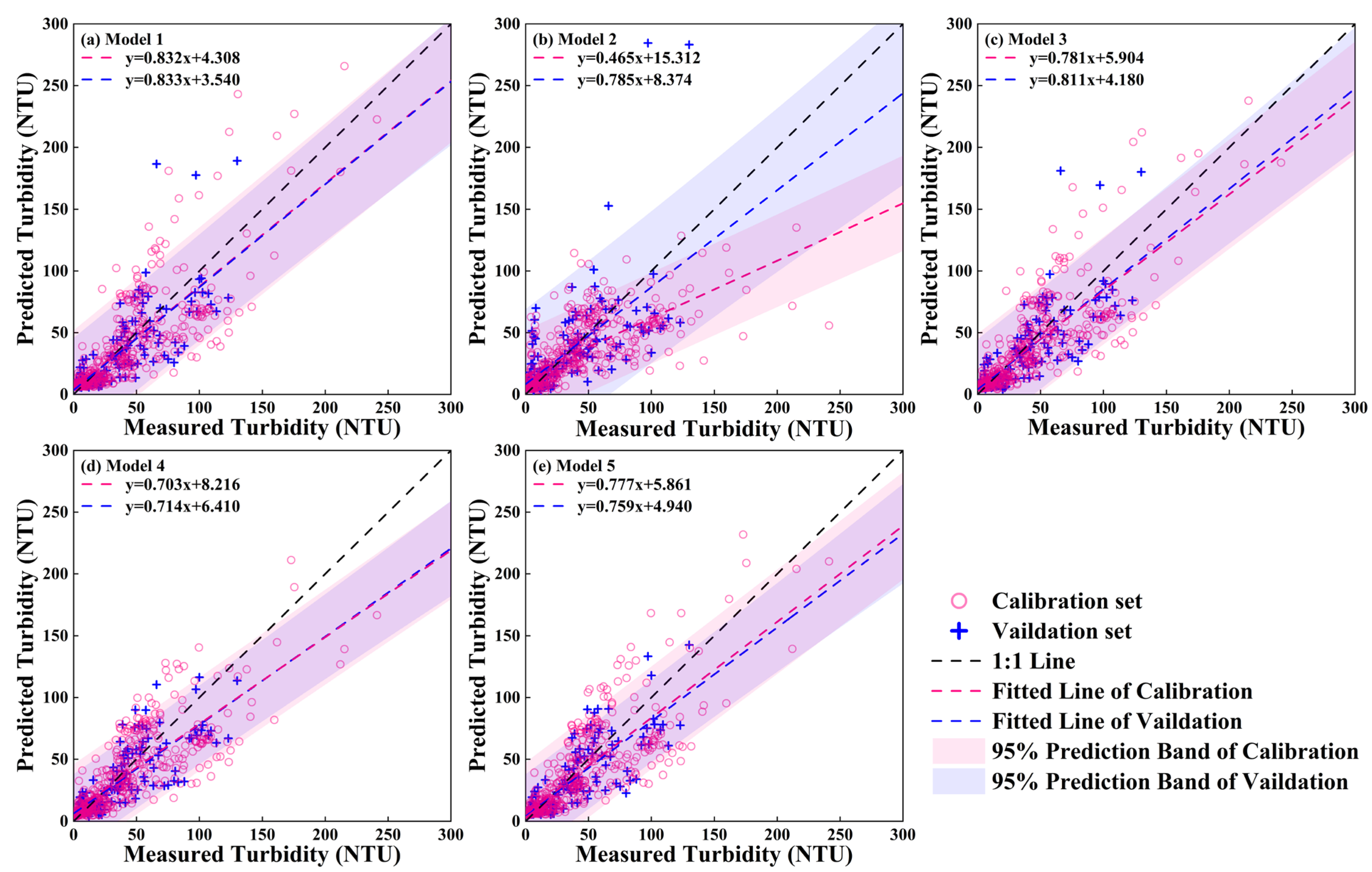
Note: B1, B2, B3, B5, and B6 represent blue, green, red, shortwave infrared 1 and shortwave infrared 2 surface reflectance, respectively.

shows five multiple linear stepwise regression models and their prediction accuracy using different reflectance variables. Model 2 produced the lowest accuracies, with the lowest R² value below 0.5 and the highest RMSE and MAE values. Model 3 outperformed Model 1 by utilizing the same three bands (blue, red, and SWIR1). But Model 3 used both single-band and band-ratio variables and achieved improved accuracy. In the validation set, Model 5 (R² = 0.676 and RMSE = 18.432 NTU) slightly outperformed Model 4 (R² = 0.669 and RMSE = 18.457 NTU) by integrating three visible bands and one shortwave infrared band, achieving higher slope values of 0.777 (Table 2 and Figure 4e) The final equation of Model 5 was composed exclusively of band difference variables selected through multiple linear stepwise regression. Although the simplified equation of Model 5 was a linear combination of single bands (blue, green, red, and SWIR1), it still demonstrated superior performance compared to Model 1.

3.3. Spatiotemporal Patterns of Turbidity

Figure 5a–e present the annual average turbidity maps for lakes in the study area from 1985 to 2023, revealing distinct spatial distribution patterns of water turbidity. The results indicated that lakes with lower turbidity (0–10 NTU) were relatively few, increasing from 1.46% in 1985 to 5.34% in 2023, with a peak of 6.80% in 2015. Lakes with turbidity levels ranging from 10 to 30 NTU remained dominant throughout the period, accounting for 29.13%, 35.44%, 30.10%, 33.01%, and 35.92% of the total in 1985, 1995, 2005, 2015, and 2023, respectively. High-turbidity lakes (greater than 150 NTU) constituted the smallest proportion, decreasing from 12.14% in 1985 to 3.40% in 2023. Moreover, lakes with different turbidity levels changed significantly before 2005, whereas variations moderated and the number of low-turbidity lakes increased during 2015–2023. Lakes with turbidity greater than 30 NTU were predominantly located in the Songnen and the Sanjiang Plains, whereas the remaining regions were primarily characterized by low-turbidity lakes. Figure 5f shows the annual average turbidity trends from 1985 to 2023. In the study area, 69.90% of lakes showed a decreasing trend, while 30.09% experienced increasing trends. A significant decrease in turbidity was observed in 10.68% of water bodies, while 2.91% demonstrated significant increases. Spatially, the regions with significantly increased turbidity were primarily located in the Songnen and the Sanjiang Plains.

3.4. Spatiotemporal Patterns of Turbidity Coefficient of Variation

From 1985 to 2023, most lakes exhibited relatively low CVs (primarily 0 to 0.4) for turbidity. Specifically, 58.74%, 72.33%, 62.14%, 72.33%, and 82.52% of the lakes showed CV < 0.4 in 1985, 1995, 2005, 2015, and 2023, with an increasing trend overall. In 1985, 13.59% of the lakes showed CV > 1 in the northern part of the study area, which significantly decreased to 1.46% in 2023. By 2023, over 80% of the lakes exhibited 0 < CV < 0.4. Lakes with CV > 0.4 were mainly concentrated in the Songnen and Sanjiang Plains near Lake Khanka from 1985 to 2023. Most water bodies exhibited a decreasing internal turbidity heterogeneity (Figure 6f). Specifically, 70.87% of the lakes showed decreasing CVs for turbidity, while 29.13% exhibited an increasing trend. Notably, 0.97% of the lakes exhibited a significant increase in CV for turbidity, while 5.34% showed a notable decrease. The lakes showing increasing spatial heterogeneity for turbidity CV were mainly distributed in the Songnen Plain of western Jilin and Heilongjiang Provinces, as well as near Lake Khanka in the Sanjiang Plain of eastern Heilongjiang.

3.5. Driving Factors for Turbidity

3.5.1. Hydrological Factors Based on Statistical Data Analysis

Figure 7 illustrates distinct gradient variations in turbidity relative to three hydrological factors: lake area, depth, and volume. It also illustrated the spatial distribution of three hydrological factors. The results demonstrated negative correlations between these three hydrological variables and turbidity. Specifically, mean water depth exhibited the strongest correlation with turbidity (R² = 0.894), followed by mean volume (R² = 0.882). As shown in Figure 7c,d, the water depth and volume are below 2 m and 0.02 km³, respectively, with the higher average turbidity exceeding 60 NTU. Thus, shallow small-volume lakes exhibited higher turbidity, which were predominantly situated in the Songnen Plain of Jilin Province. However, mean surface area exhibited a weaker correlation (R² = 0.675). Lakes above 200 km² exhibited relatively high average turbidity exceeding 40 NTU. Hence, the lake surface area was not the dominant driving factor of turbidity variations, whereas water depth demonstrated significant effects.

3.5.2. Spatiotemporal Influence of Environmental Factors Based on GTWR

As shown in

Table 3. Spatial autocorrelation results of water turbidity at the watershed scale.

Measurement Index	Year
	1985	1995	2005	2015	2023
Moran’s I index	0.108	0.105	0.148	0.203	0.183
z-score	2.362	2.348	3.104	4.203	3.713
p-value	0.018	0.019	0.002	0.000	0.000

, the Moran’s I indices of water turbidity at the watershed scale in Northeast China for 1985, 1995, 2005, 2015, and 2023 were 0.108, 0.105, 0.148, 0.203, and 0.1831, respectively (Table 2). All p-values were less than 0.05, and the standardized Z-scores exceeded 1.96, which corresponded to the 95% significance level under a normal distribution. These results indicated a significant positive spatial correlation in water turbidity at the watershed scale in Northeast China. The spatial autocorrelation results confirmed the necessity of applying geographic weighting for the regression analysis of this dataset.

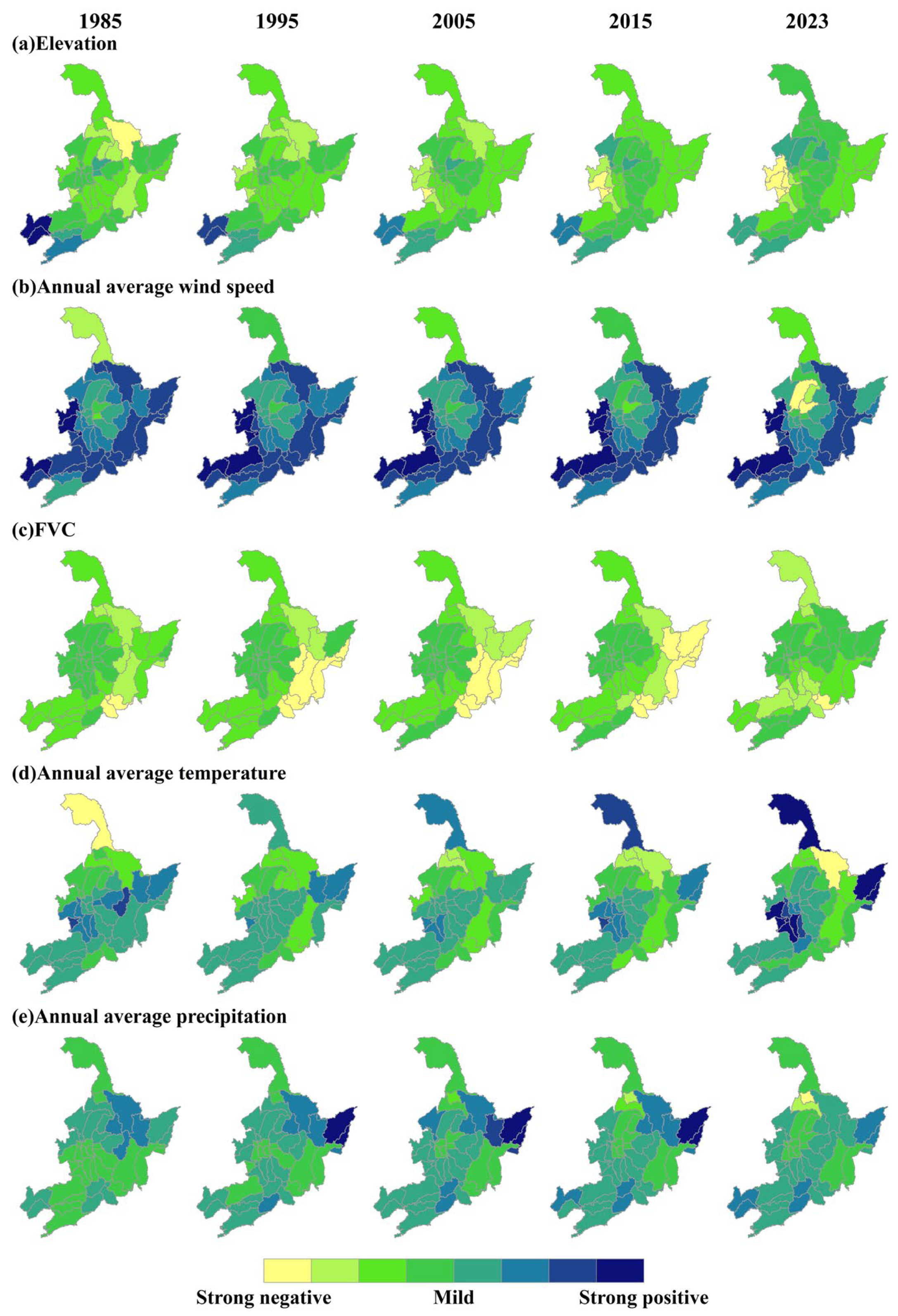
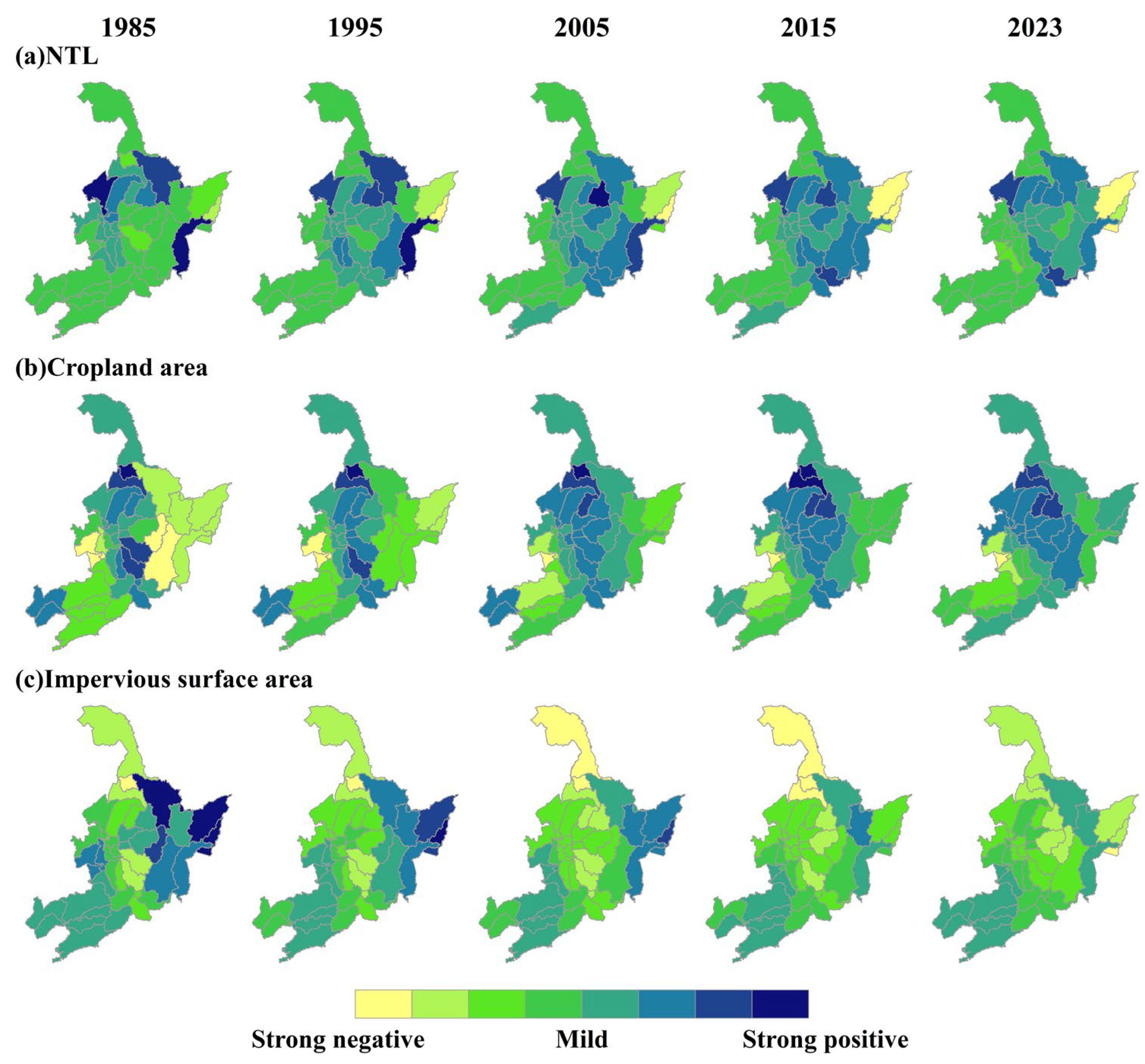
Figure 8 and Figure 9 illustrate the spatiotemporal patterns of GTWR-derived standardized regression coefficients for natural and anthropogenic factors from 1985 to 2023. The distinct regression coefficients of various driving factors were classified into eight correlation intensity levels. Terrain factors negatively correlated with the spatiotemporal variations in turbidity. In the Eastern Mountains region (watersheds 19, 25, 28, 29, 30, 31, and 36), elevation demonstrated obvious negative impacts on turbidity and remained stable (Figure 8a). Wind speed showed a consistently positive effect on turbidity, particularly in the western watersheds of the Songnen Plain (watersheds 13, 21, 33, 35, and 41). Its influence maintained strong positive correlation across the spatial scale over the study period (Figure 8b). Vegetation coverage exhibited a negative effect on turbidity, with gradually strengthening negative effects from west to east. In particular, the watersheds in the Eastern Mountains region (14, 19, 25, 29, 30, and 31) showed strong responses from 1995 to 2015 (Figure 8c). Temperature showed a positive correlation with turbidity, especially in the Songnen, Sanjiang, and Liaohe Plain watersheds, where the strongest positive correlation was observed. This relationship intensified gradually since 1985 and peaked in 2023 (Figure 8d). Precipitation exhibited a positive correlation with turbidity, which was particularly evident in the watersheds of Sanjiang Plain (Figure 8e).

The association between NTL and water turbidity remained stable. Spatially, the positive correlations concentrated in the Songnen Plain watersheds, predominantly urban development areas, including watersheds 3, 6, 7, 9, and 10 (Figure 9a). Cropland area correlated positively with turbidity, predominantly in the northern part of the Songnen Plain region, with its influence expanding since 1985 (Figure 9b). Impervious surface area moderately correlated with water turbidity. Strong correlations were observed in the eastern watersheds (5, 8, 19, 37, and 38) between 1985 and 2005, which weakened since 2015 (Figure 9c). Compared to NTL, however, the relationship between impervious surface area and turbidity was not significant.

Furthermore, the GTWR-derived regression coefficients for various driving factors in each watershed demonstrated their temporal influence on turbidity variations (Figure 10). Elevation showed a consistently negative effect on turbidity, with the mean regression coefficients remaining stable at approximately −0.285 over the study period (Figure 10a). The mean regression coefficients of FVC showed a downward trend from 1985 to 2015, suggesting a strengthening negative impact of vegetation coverage on turbidity (Figure 10b). Annual average wind speed exhibited an overall slightly decreasing positive effect on turbidity, and the mean regression coefficients showed a fluctuating downward trend (Figure 10c). The mean regression coefficients of annual average temperature fluctuated, with a downward trend from 1985 to 2005, followed by an upward trend from 2015 to 2023 (Figure 10d). In contrast, the mean regression coefficients of annual average precipitation exhibited an opposite pattern (Figure 10e). Regarding anthropogenic factors, the mean regression coefficients of NTL and cropland area displayed steadily increasing effects on turbidity from 1985 to 2015, followed by a slight decline by 2023 (Figure 10f,g). The mean regression coefficients of impervious surface area showed a downward trend (Figure 10h). Additionally, the fluctuation interval of regression coefficients for annual average wind speed, temperature, and precipitation showed an expanding trend, while that for NTL and impervious surface area exhibited a shrinking trend.

3.5.3. Contribution Rates of the Driving Factors Based on the LMG Method

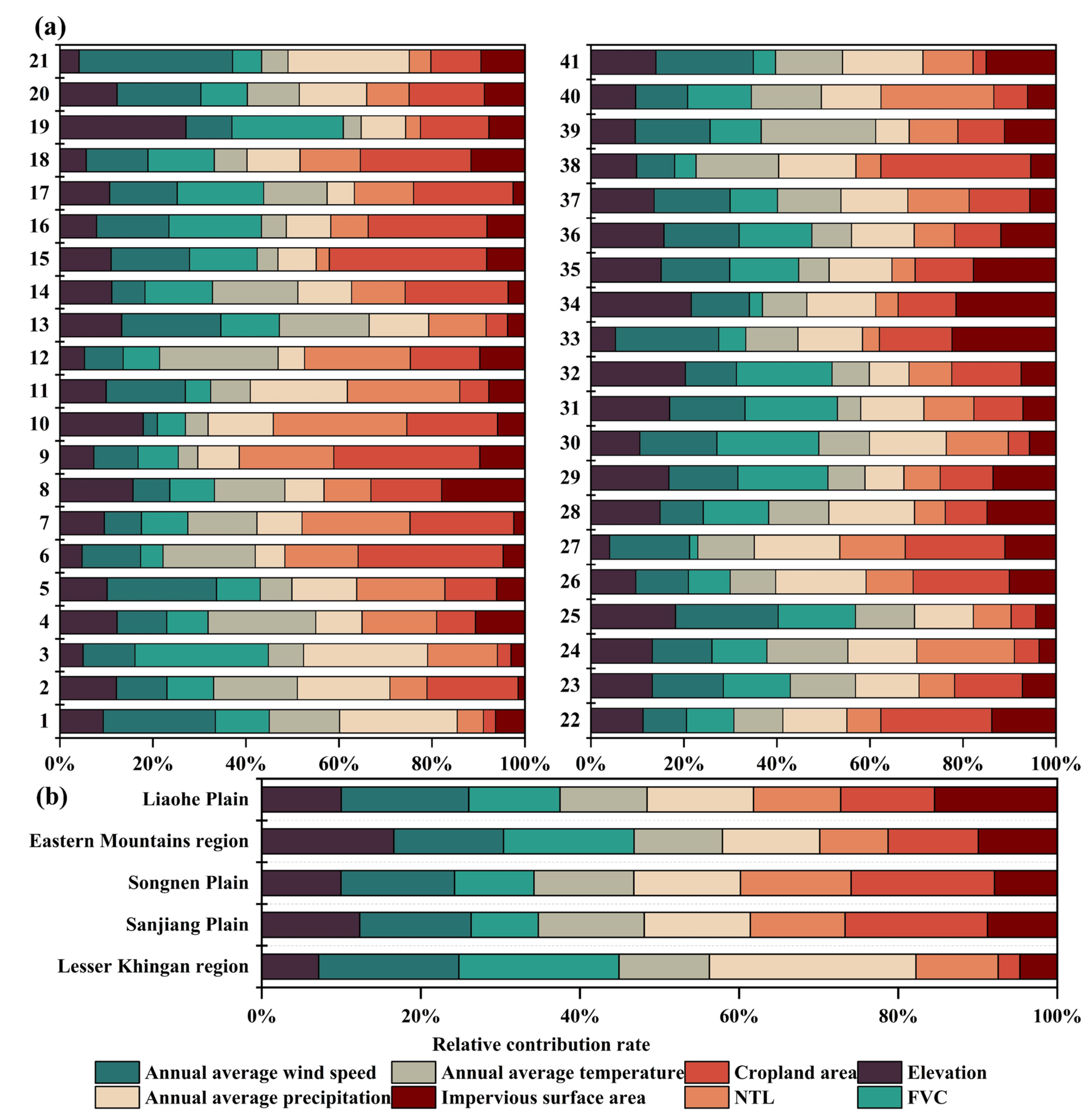
Figure 11 shows that the LMG-derived contribution rates of various factors driving turbidity variations differ significantly among watersheds over the past 40 years. Vegetation coverage and precipitation were the primary factors in the Lesser Khingan Mountains region (watersheds 1 and 3), with mean contribution rates of 20.13% and 25.96%, respectively. Watersheds 5, 8, 37, and 38 in the Sanjiang Plain demonstrated the higher mean contribution rates of wind speed and cropland area (>14%). Temperature and precipitation also contributed significantly to turbidity variations in watersheds 37 and 38. In the Eastern Mountains region, the mean contribution rate of elevation was the highest at 16.60%, followed by that of vegetation coverage at 16.39% and wind speed at 13.79% (Figure 11b). Moreover, anthropogenic factors like cropland area and impervious surface area explained turbidity variations well in watersheds 14, 19, 28, 32, 34, and 39 in the Eastern Mountains region near the plain region, with rates of 22.16% (cropland area) and 21.53% (impervious surface area). Wind speed significantly influenced turbidity variations in the Liaohe Plain, with a mean contribution rate of 16.03%, especially in watershed 33. Vegetation coverage had the highest average contribution rate (14.84%) in watershed 35 of the Liaohe Plain, whereas anthropogenic factors (i.e., cropland area, impervious surface area, and NTL) significantly influenced turbidity in watersheds 33, 35, and 40. Wind speed contributed to turbidity variations as a dominant driving factor in watersheds 13, 20, 21, 23, and 41, predominantly situated in the Songnen Plain of Jilin Province, with rates ranging from 15.29% to 32.97%. Cropland area emerged as the most significant driving factor, with the highest mean contribution rate of 18.00% in the Songnen Plain. In addition, temperature and precipitation also played crucial roles in explaining water turbidity variations, especially in watersheds 13, 20, 22, 23, 24, 27, and 41 within the Songnen Plain of Jilin Province, with contribution rates exceeding 10%.

Figure 12 presents the mean contribution rates of natural and anthropogenic factors in each watershed based on the LMG method. Among the 41 watersheds in Northeast China, natural factors predominantly contributed to turbidity variations in 24 watersheds, while the contributions of anthropogenic factors were dominant in 17 watersheds. As shown in Figure 12, the effects of natural factors on turbidity significantly outweigh anthropogenic factors in the Lesser Khingan Mountains region (16.44% vs. 5.93%) and Eastern Mountains region (14.03% vs. 9.95%). The anthropogenic factors played a more significant role in the Sanjiang, Liaohe and Songnen Plains, with contribution rates of 12.86%, 12.73% and 13.28%, respectively.

4. Discussion

4.1. Model Assessment and Turbidity Mapping

The developed multiple linear stepwise regression model employed a linear combination of visible and shortwave infrared spectral reflectance to produce credible estimations of turbidity. The selected spectral bands with regression coefficients exhibited marked differences between the red band and other bands, which corresponded to the characteristics of Case II waters and were sensitive to water turbidity. Multiple linear stepwise regression effectively and automatically determined significant variables for model building. In this study, the method removed band-ratio variables and retained band difference variables to form a single-band model. This study proved that the multiple linear stepwise regression model is more practical for estimating lake turbidity and is more efficient in mapping the long-term and large-scale spatiotemporal distribution patterns of turbidity.

However, it posed significant challenges to developing a highly accurate linear regression model, which used samples from diverse water bodies with high spatial heterogeneity in the large-scale study area. Previous studies also demonstrated that the regression model could be effectively used for large-scale turbidity mapping, but the accuracy was generally not high compared to machine learning methods [5,15,41]. The model in this study yielded a relatively better results compared to other studies. But the accuracy assessment placed the estimation bias in the high-value range, potentially due to the insufficient samples and the model’s limitations in capturing the relationship between surface reflectance and turbidity. More effort should be devoted to in situ data collection to acquire sufficient samples for model development and performance improvement.

Furthermore, the generated spatial maps of turbidity demonstrated significant variations in distribution patterns and temporal dynamics. In terms of temporal turbidity variations, an overall decreasing trend was observed in the number of lakes with high turbidity. From 1985 to 2015, a relatively large number of high-turbidity lakes exhibited significant turbidity changes. After 2015, turbidity variations became relatively slower, and the number of low-turbidity lakes increased significantly. The spatial variations in the mean and CV of turbidity revealed that lakes with significantly increased turbidity and internal spatial heterogeneity were predominantly concentrated in the Songnen and Sanjiang Plains. In contrast, lakes with lower turbidity were situated in the Eastern Mountains regions and the Liaohe Plain over the past 40 years. The significant turbidity variations were likely due to the regional economic development, characterized by rapid population growth, urban expansion, and frequent industrial and agricultural activities, which affected water environment conditions. The water environment treatment measures supported by local governments helped mitigate the water quality decline.

4.2. Influence of Driving Factors on Long-Term Turbidity Variations

The assessment of factors driving turbidity variations integrated statistical data analysis, GTWR, and the LMG method, thus effectively revealing their spatiotemporal distribution patterns and contributions. The results demonstrated that the impact of various hydrological, anthropogenic, and natural factors on turbidity variations exhibited spatiotemporal heterogeneity. In terms of the temporal influence on turbidity variations, elevation, as a stable geographic element, exerted a relatively consistent influence on the interannual turbidity variations. The vegetation coverage and anthropogenic factors (i.e., cropland area and NTL) showed increasingly strong impacts on turbidity from 1985 to 2015, and the degree of influence decreased from 2015 to 2023. This may be due to the increase in forest area under government afforestation policies, rapid population growth, urban expansion, and intensive agricultural and industrial activities during the rapid socioeconomic development from 1985 to 2015. The expanding fluctuation interval of coefficients for climate driving factors (i.e., wind speed, temperature, and precipitation) highlighted that the spatially heterogeneous impact on turbidity continuously increased over time, which was especially significant with temperature. Overall, the influence intensity of all environmental driving factors except elevation decreased after 2015. This may be because various national and local government policies intended to strengthen water environment management were introduced after 2015, which restricted human activities to control the discharge of industrial, agricultural, and domestic sewage. Under anthropogenic interference, the water quality improved, and the variations stabilized, suggesting the weakening impacts of these environmental factors [5,62,63,64].

In terms of spatial influence, the low-turbidity lakes in Northern China are predominantly found in the Liaohe Plain and Eastern Mountains region, whereas high-turbidity lakes are distributed in the Songnen and Sanjiang Plains. In the Eastern Mountains region with high elevation, several low-turbidity lakes surrounded by high mountains or hills were endowed with greater storage capacities and depths, which effectively resisted disturbances from strong winds and water flow, resulting in enhanced sedimentation of suspended particles and decreased turbidity. Meanwhile, the lakes of the high-elevation region are rarely disturbed by human activities, resulting in high water clarity [30]. In addition to elevation, vegetation coverage also significantly negatively influenced turbidity according to the contribution analysis using the LMG method, thus effectively avoiding soil erosion. The Lesser Khingan Mountains region shared similar geographical characteristics with the Eastern Mountains region, where high vegetation coverage significantly influenced turbidity. Moreover, several large water bodies in the Eastern Mountains region also functioned as reservoirs, providing water for domestic use, irrigation, and aquaculture. The water quality was effectively protected through human intervention measures, contributing to the sustained low turbidity [65].

Lakes with high turbidity are predominantly concentrated in the low-elevation areas of the Songnen Plain. This result is consistent with the findings on the spatial variation in lakes with high clarity in the Songnen Plain, as demonstrated by Song et al. (2020) [66]. Songnen Plain hosts important grain production bases and urban development areas for human settlement. Thus, the several lakes are surrounded by extensive agricultural land and built-up areas. Water bodies near agricultural areas are often exposed to soil erosion, with sediment being carried into lakes [67,68,69]. Previous studies have demonstrated that lakes surrounded by farmland exhibited high TSM [70]. The GTWR and LMG findings in this study showed that anthropogenic factors contributed more significantly than natural factors to turbidity variations in the Songnen Plain. Frequent agricultural activities (e.g., tillage, seeding, and weeding) and urban expansion induced intensive soil disturbances. Soil particles are easily transported into nearby lakes via surface runoff during precipitation, leading to increased lake turbidity. Moreover, nutrients from agricultural fertilizer or wastewater discharge (i.e., industrial and sanitary sewage) dramatically promote the growth of algae and plankton, leading to increased organic particulate matter. Tao et al. (2022) demonstrated agricultural fertilizer use as one of the important factors affecting lake clarity [71]. Anthropogenic factors also exerted an obvious impact on water turbidity in the Sanjiang and Liaohe Plains with extensive croplands and impervious surfaces, suggesting the presence of frequent human activities.

In addition, GTWR results indicated that temperature positively contributed to lake turbidity variations in the southern Songnen Plain. Increased temperatures promote the growth and proliferation of phytoplankton and algae [62,72,73]. Thus, shallow and small lakes in this region may undergo eutrophication due to their favorable light conditions for photosynthesis and rising temperatures, leading to elevated turbidity. Wind speed is another critical factor influencing turbidity variations. GTWR results indicated that wind speed significantly affected the turbidity in the western watersheds of the Songnen Plain. Numerous shallow lakes with high turbidity are predominantly found in this region, which are highly susceptible to wind speed variations. High wind speeds enhance water turbulence and resuspend sediment, thus increasing turbidity. Wind speed also exhibited high contribution rates to lake turbidity in Sanjiang and Liaohe Plains.

4.3. Uncertainty Analysis and Future Perspectives

This paper proposed regression model for turbidity estimation and mapping. The prediction accuracy had the potential to be significantly improved. The collection of sufficient samples and the development of advanced models (e.g., machine learning models and deep learning models) are essential tasks that need to be prioritized and carried out in future research. Moreover, more efforts should be devoted to supplementing seasonal data to enable detailed analysis of the spatial dynamics of water turbidity.

GTWR and LMG models effectively illustrated the spatiotemporal influence patterns and overall contributions of various driving factors at the watershed scale. However, the performance of these models can be affected by the input datasets and the interactions between independent variables (i.e., various driving factors). Generally, the GTWR model may somewhat diminish the possible heterogeneity in the scale of correlation among variables, thus failing to fully reveal the response mechanisms in local watersheds. Specifically, the independent and dependent variables were derived from the mean values of driving factor data and annual turbidity within a watershed. Due to the nonuniform spatial distribution of water bodies and the inconsistent scales of multiple driving factor datasets, the correspondence between turbidity and driving factors is limited. Due to challenges in acquiring some driving factor datasets that fully covered the research period, the nearest available year was used to fill data gaps. This approach, which was predominantly applied prior to 1995, heightened such uncertainty during that period. Additionally, this study determined watershed scales by comprehensively considering water body distribution patterns and natural geographic characteristics. The limited number of watersheds resulted in insufficient samples for the GTWR and LMG models, limiting their ability to explain driving factors and inducing biases in the assessments of such driving factors in some watersheds.

Future research may direct more efforts to enhance model interpretability by increasing the number of water bodies for evaluation, refining driving factor data, filling missing factor data via multi-source data fusion, and optimizing watershed delineation. Moreover, the natural and anthropogenic factors affecting turbidity are quite complex, and accurately and fully quantifying their influence on turbidity remains a challenge. Subsequent research should integrate more data on potential driving factors to identify more factors influencing water turbidity.

5. Conclusions

Using Landsat data from 1985 to 2023, this study developed a multiple linear stepwise regression model to estimate the turbidity of 206 lakes above 5 km² in Northern China. The stepwise regression model was able to credibly estimate turbidity, achieving a low RMSE of 18.432 NTU. Annual turbidity maps were generated and applied to explore the spatiotemporal dynamics of turbidity. The impacts of hydrological, anthropogenic, and natural factors on the spatiotemporal variations in lake turbidity at the watershed scale in various geographical regions were investigated based on statistical data analysis, GTWR, and the LMG method.

The long-term monitoring revealed significant variations in distribution patterns and temporal dynamics of lake turbidity in Northern China. Temporal turbidity variations showed an overall decreasing trend. The spatial variations revealed significantly increased turbidities predominantly in the Songnen and Sanjiang Plains and lower turbidities in the Eastern Mountains and Liaohe Plain over the past 40 years.

The statistical data analysis of hydrological factors showed that water depth is significantly related to water turbidity variations. Moreover, the assessment based on GTWR and the LMG method demonstrated that the natural and anthropogenic factors driving turbidity variations showed significant spatiotemporal heterogeneity. The temporal variations showed obvious fluctuations, with the influence of environmental factors strengthening from 1985 to 2015 and weakening after 2015, consistent with the pattern of socioeconomic development and government interventions on the water environment.

The mean contribution rates of the primary influencing factors exhibited significant differences across regions. FVC (20.13%) and precipitation (25.96%) were the main factors influencing turbidity in the Lesser Khingan Mountains region. In the Eastern Mountains regions, elevation (16.60%) and FVC (16.39%) were the dominant factors. In the Songnen and Sanjiang Plains, cropland area (18.00% and 17.89%) and wind speed (14.25% and 14.00%) proved the primary factors influencing turbidity, while wind speed (16.03%) and impervious surface area (15.43%) were key factors in the Liaohe Plain.

Overall, the impacts of natural factors on turbidity significantly outweighed anthropogenic factors in the Lesser Khingan Mountains and Eastern Mountains regions. The anthropogenic factors played more significant roles in the Sanjiang, Liaohe and Songnen Plains. These findings contribute to informed decision-making in water environment management and the sustainable development of aquatic ecosystems under the influences of human activities and climate change.

References

1. Gleick, P.H. Global freshwater resources: Soft-path solutions for the 21st century. Science 2003, 302, 1524–1528. [Google Scholar] [CrossRef] [PubMed]
2. Pekel, J.F.; Cottam, A.; Gorelick, N.; Belward, A.S. High-resolution mapping of global surface water and its long-term changes. Nature 2016, 540, 418–422. [Google Scholar] [CrossRef] [PubMed]
3. Kuhn, C.; de Matos Valerio, A.; Ward, N.; Loken, L.; Sawakuchi, H.O.; Kampel, M.; Richey, J.; Stadler, P.; Crawford, J.; Striegl, R.; et al. Performance of Landsat-8 and Sentinel-2 surface reflectance products for river remote sensing retrievals of chlorophyll-a and turbidity. Remote Sens. Environ. 2019, 224, 104–118. [Google Scholar] [CrossRef]
4. Deng, X.Y.; Song, C.Q.; Liu, K.; Ke, L.H.; Zhang, W.S.; Ma, R.H.; Zhu, J.Y.; Wu, Q.H. Remote sensing estimation of catchment-scale reservoir water impoundment in the upper yellow river and implications for river discharge alteration. J. Hydrol. 2020, 585, 124791. [Google Scholar] [CrossRef]
5. Zhang, L.; Xin, Z.H.; Feng, L.; Hu, C.M.; Zhou, H.C.; Wang, Y.; Song, C.C.; Zhang, C. Turbidity dynamics of large lakes and reservoirs in northeastern China in response to natural factors and human activities. J. Clean. Prod. 2022, 368, 133148. [Google Scholar] [CrossRef]
6. Zhang, K.; Li, L.J.; Bai, P.; Li, J.Y.; Liu, Y.M. Influence of climate variability and human activities on stream flow variation in the past 50 years in Taoer River, Northeast China. J. Geogr. Sci. 2017, 27, 481–496. [Google Scholar] [CrossRef]
7. Xu, H.; Paerl, H.W.; Qin, B.; Zhu, G.; Hall, N.S.; Wu, Y. Determining critical nutrient thresholds needed to control harmful cyanobacterial blooms in eutrophic Lake Taihu, China. Environ. Sci. Technol. 2015, 49, 1051–1059. [Google Scholar] [CrossRef]
8. Carey, C.C.; Ibelings, B.W.; Hoffmann, E.P.; Hamilton, D.P.; Brookes, J.D. Eco-physiological adaptations that favour freshwater cyanobacteria in a changing climate. Water Res. 2012, 46, 1394–1407. [Google Scholar] [CrossRef]
9. Huisman, J.; Codd, G.A.; Paerl, H.W.; Ibelings, B.W.; Verspagen, J.M.; Visser, P.M. Cyanobacterial blooms. Nat. Rev. Microbiol. 2018, 16, 471–483. [Google Scholar] [CrossRef]
10. Davies-Colley, R.J.; Smith, D.G. Turbidity suspeni)ed sediment, and water clarity: A review. J. Am. Water Resour. Assoc. 2001, 37, 1085–1101. [Google Scholar] [CrossRef]
11. Ayana, E. Determinants of Declining Water Quality; World Bank Group: Washington, DC, USA, 2019. [Google Scholar]
12. Gao, P.; Pasternack, G.B.; Bali, K.M.; Wallender, W.W. Estimating suspended sediment concentration using turbidity in an irrigation-dominated southeastern California watershed. J. Irrig. Drain. Eng. 2008, 134, 250–259. [Google Scholar] [CrossRef]
13. McCarthy, M.J.; Muller-Karger, F.E.; Otis, D.B.; Méndez-Lázaro, P. Impacts of 40 years of land cover change on water quality in Tampa Bay, Florida. Cogent Geosci. 2018, 4, 1422956. [Google Scholar] [CrossRef]
14. Dogliotti, A.I.; Ruddick, K.G.; Nechad, B.; Doxaran, D.; Knaeps, E. A single algorithm to retrieve turbidity from remotely-sensed data in all coastal and estuarine waters. Remote Sens. Environ. 2015, 156, 157–168. [Google Scholar] [CrossRef]
15. Li, Y.; Li, S.J.; Song, K.S.; Liu, G.; Wen, Z.D.; Fang, C.; Shang, Y.X.; Lyu, L.L.; Zhang, L.L. Sentinel-3 OLCI observations of Chinese lake turbidity using machine learning algorithms. J. Hydrol. 2023, 622, 129668. [Google Scholar] [CrossRef]
16. Sipelgas, L.; Raudsepp, U.; Kõuts, T. Operational monitoring of suspended matter distribution using MODIS images and numerical modelling. Adv. Space Res. 2006, 38, 2182–2188. [Google Scholar] [CrossRef]
17. Duan, W.; Takara, K.; He, B.; Luo, P.; Nover, D.; Yamashiki, Y. Spatial and temporal trends in estimates of nutrient and suspended sediment loads in the Ishikari River, Japan, 1985 to 2010. Sci. Total Environ. 2013, 461–462, 499–508. [Google Scholar] [CrossRef]
18. Caballero, I.; Navarro, G.; Ruiz, J. Multi-platform assessment of turbidity plumes during dredging operations in a major estuarine system. Int. J. Appl. Earth Obs. 2018, 68, 31–41. [Google Scholar] [CrossRef]
19. Peterson, K.T.; Sagan, V.; Sloan, J.J. Deep learning-based water quality estimation and anomaly detection using Landsat-8/Sentinel-2 virtual constellation and cloud computing. GISci. Remote Sens. 2020, 57, 510–525. [Google Scholar] [CrossRef]
20. Bustamante, J.; Pacios, F.; Diaz-Delgado, R.; Aragones, D. Predictive models of turbidity and water depth in the Doana marshes using Landsat TM and ETM+ images. J. Environ. Manag. 2009, 90, 2219–2225. [Google Scholar] [CrossRef]
21. Jiang, X.Z.; Lu, B.; He, Y.H. Response of the turbidity maximum zone to fluctuations in sediment discharge from river to estuary in the Changjiang Estuary (China). Estuar. Coast. Shelf Sci. 2013, 131, 24–30. [Google Scholar] [CrossRef]
22. Shen, X.; Feng, Q. Statistical model and estimation of inland riverine turbidity with Landsat 8 OLI images: A case study. Environ. Eng. Sci. 2018, 35, 132–140. [Google Scholar] [CrossRef]
23. Erena, M.; Domínguez, J.A.; Aguado-Giménez, F.; Soria, J.; García-Galiano, S. Monitoring Coastal Lagoon Water Quality through Remote Sensing: The Mar Menor as a Case Study. Water 2019, 11, 1468. [Google Scholar] [CrossRef]
24. Sebastiá-Frasquet, M.-T.; Aguilar-Maldonado, J.A.; Santamaría-Del-Ángel, E.; Estornell, J. Sentinel 2 Analysis of Turbidity Patterns in a Coastal Lagoon. Remote Sens. 2019, 11, 2926. [Google Scholar] [CrossRef]
25. Doxaran, D.; Froidefond, J.M.; Castaing, P.; Babin, M. Dynamics of the turbidity maximum zone in a macrotidal estuary (the Gironde, France): Observations from field and MODIS satellite data. Estuar. Coast. Shelf Sci. 2009, 81, 321–332. [Google Scholar] [CrossRef]
26. Petus, C.; Chust, G.; Gohin, F.; Doxaran, D.; Froidefond, J.M.; Sagarminaga, Y. Estimating turbidity and total suspended matter in the Adour River plume (South Bay of Biscay) using MODIS 250-m imagery. Cont. Shelf Res. 2010, 30, 379–392. [Google Scholar] [CrossRef]
27. Urquhart, E.A.; Schaeffer, B.A. Envisat MERIS and Sentinel-3 OLCI satellite lake biophysical water quality flag dataset for the contiguous United States. Data Brief 2020, 28, 104826. [Google Scholar] [CrossRef]
28. Wang, S.Q.; Mao, Y.; Zheng, L.F.; Qiu, Z.F.; Bilal, M.; Sun, D.Y. Remote sensing of water turbidity in the eastern China seas from geostationary ocean colour imager. Int. J. Remote Sens. 2020, 41, 4080–4101. [Google Scholar] [CrossRef]
29. Wu, D.F.; Tang, T.; Odermatt, D.; Liu, W.F. Spatiotemporal variability in global lakes turbidity derived from satellite imageries. Environ. Res. Commun. 2025, 7, 035007. [Google Scholar] [CrossRef]
30. Song, K.S.; Wang, Q.; Liu, G.; Jacinthe, P.A.; Li, S.J.; Tao, H.; Du, Y.X.; Wen, Z.D.; Wang, X.; Guo, W.W.; et al. A unified model for high resolution mapping of global lake (>1 ha) clarity using Landsat imagery data. Sci. Total Environ. 2022, 810, 151188. [Google Scholar] [CrossRef]
31. Zhang, Y.Z.; Pulliainen, J.T.; Koponen, S.S.; Hallikainen, M.T. Water quality retrievals from combined Landsat TM data and ERS-2 SAR data in the Gulf of Finland. IEEE Trans. Geosci. Remote 2003, 41, 622–629. [Google Scholar] [CrossRef]
32. Silveira Kupssinskü, L.; Thomassim Guimarães, T.; Menezes de Souza, E.; Zanotta, D.C.; Roberto Veronez, M.; Gonzaga, L., Jr.; Mauad, F.F. A Method for Chlorophyll-a and Suspended Solids Prediction through Remote Sensing and Machine Learning. Sensors 2020, 20, 2125. [Google Scholar] [CrossRef]
33. Wang, Y.F.; Chen, J.; Cai, H.; Yu, Q.; Zhou, Z. Predicting water turbidity in a macro-tidal coastal bay using machine learning approaches. Estuar. Coast. Shelf Sci. 2021, 252, 107276. [Google Scholar] [CrossRef]
34. Wan, S.; Yeh, M.L.; Ma, H.L.; Chou, T.Y. The Robust Study of Deep Learning Recursive Neural Network for Predicting of Turbidity of Water. Water 2022, 14, 761. [Google Scholar] [CrossRef]
35. Kumar, L.; Afzal, M.S.; Ahmad, A. Prediction of water turbidity in a marine environment using machine learning: A case study of Hong Kong. Reg. Stud. Mar. Sci. 2022, 52, 102260. [Google Scholar] [CrossRef]
36. Palmer, S.C.; Kutser, T.; Hunter, P.D. Remote sensing of inland waters: Challenges, progress and future directions. Remote Sens. Environ. 2015, 157, 1–8. [Google Scholar] [CrossRef]
37. Wischmeier, W.H.; Smith, D.D. Predicting Rainfall Erosion Losses: A Guide to Conservation Planning; Department of Agriculture, Science and Education Administration: Washington, DC, USA, 1978. [Google Scholar]
38. Yang, S.L.; Wang, J.; Cong, W.; Cai, Z.L.; Ouyang, F. Utilization of nitrite as a nitrogen source by Botryococcus braunii. Biotechnol. Lett. 2004, 26, 239–243. [Google Scholar] [CrossRef]
39. Ouyang, T.P.; Zhu, Z.Y.; Kuang, Y.Q. Assessing impact of urbanization on river water quality in the Pearl River Delta Economic Zone, China. Environ. Monit. Assess. 2006, 120, 313–325. [Google Scholar] [CrossRef]
40. Uriarte, M.; Yackulic, C.B.; Lim, Y.; Arce-Nazario, J.A. Influence of land use on water quality in a tropical landscape: A multi-scale analysis. Landscape Ecol. 2011, 26, 1151–1164. [Google Scholar] [CrossRef]
41. Li, S.J.; Kutser, T.; Song, K.S.; Liu, G.; Li, Y. Lake Turbidity Mapping Using an OWTs-bp Based Framework and Sentinel-2 Imagery. Remote Sens. 2023, 15, 2489. [Google Scholar] [CrossRef]
42. Wang, X.D.; Song, K.S.; Wen, Z.D.; Liu, G.; Shang, Y.X.; Fang, C.; Lyu, L.L.; Wang, Q. Quantifying turbidity variation for lakes in Daqing of Northeast China using Landsat images from 1984 to 2018. IEEE J. Sel. Top. Appl. Earth Obs. Remote Sens. 2021, 14, 8884–8897. [Google Scholar] [CrossRef]
43. Zhou, Q.; Wang, J.R.; Tian, L.Q.; Feng, L.; Li, J.; Xing, Q.G. Remotely sensed water turbidity dynamics and its potential driving factors in Wuhan, an urbanizing city of China. J. Hydrol. 2021, 593, 125893. [Google Scholar] [CrossRef]
44. Chu, H.-J.; Kong, S.-J.; Chang, C.-H. Spatio-temporal water quality mapping from satellite images using geographically and temporally weighted regression. Int. J. Appl. Earth Obs. Geoinf. 2018, 65, 1–11. [Google Scholar] [CrossRef]
45. Han, J.J.; Wang, J.P.; Chen, L.; Xiang, J.Y.; Ling, Z.Y.; Li, Q.K.; Wang, E.L. Driving factors of desertification in Qaidam Basin, China: An 18-year analysis using the geographic detector model. Ecol. Indic. 2021, 124, 107404. [Google Scholar] [CrossRef]
46. Xu, Y.D.; Pei, J.B.; Li, S.Y.; Zou, H.T.; Wang, J.K.; Zhang, J.B. Main characteristics and utilization countermeasures for black soils in different regions of Northeast China. Chin. J. Soil Sci. 2023, 54, 495–504. [Google Scholar] [CrossRef]
47. Wang, Q.; Song, K.S.; Xiao, X.M.; Jacinthe, P.-A.; Wen, Z.D.; Zhao, F.R.; Tao, H.; Li, S.J.; Shang, Y.X.; Wang, Y.; et al. Mapping water clarity in North American lakes and reservoirs using Landsat images on the GEE platform with the RGRB model. IISPRS J. Photogramm. Remote Sens. 2022, 194, 39–57. [Google Scholar] [CrossRef]
48. Xu, H.Q. A study on information extraction of water body with the modified normalized difference water index (MNDWI). J. Remote Sens. 2005, 9, 589–595. [Google Scholar] [CrossRef]
49. Otsu, N. A threshold selection method from gray-level histograms. IEEE Trans. Syst. Man Cybern. 1979, 9, 62–66. [Google Scholar] [CrossRef]
50. Tang, W.; Zhao, C.; Lin, J.; Jiao, C.; Zheng, G.; Zhu, J.; Pan, X.; Han, X. Improved Spectral Water Index Combined with Otsu Algorithm to Extract Muddy Coastline Data. Water 2022, 14, 855. [Google Scholar] [CrossRef]
51. Zhang, X.; Zhao, T.T.; Xu, H.; Liu, W.D.; Wang, J.Q.; Chen, X.D.; Liu, L.Y. GLC_FCS30D: The first global 30 m land-cover dynamics monitoring product with a fine classification system for the period from 1985 to 2022 generated using dense-time-series Landsat imagery and the continuous change-detection method. Earth Syst. Sci. Data 2024, 16, 1353–1381. [Google Scholar] [CrossRef]
52. Efroymson, M.A. Multiple regression analysis. In Mathematical Methods for Digital Computers; Wiley: Hoboken, NJ, USA, 1960; pp. 191–203. [Google Scholar]
53. Miller, A.; Panneerselvam, J.; Liu, L. A review of regression and classification techniques for analysis of common and rare variants and gene-environmental factors. Neurocomputing 2022, 489, 466–485. [Google Scholar] [CrossRef]
54. Brunsdon, C.; Charlton, F.M. Geographically weighted regression-modelling spatial non-stationarity. J. R. Stat. Soc. B 1998, 47, 431–443. [Google Scholar] [CrossRef]
55. Brunsdon, C.; Fotheringham, A.S.; Charlton, M.E. Geographically weighted regression: A method for exploring spatial nonstationarity. Geogr. Anal. 2010, 28, 281–298. [Google Scholar] [CrossRef]
56. Huang, B.; Wu, B.; Barry, M. Geographically and temporally weighted regression for modeling spatio-temporal variation in house prices. Int. J. Geogr. Inf. Sci. 2010, 24, 383–401. [Google Scholar] [CrossRef]
57. Tang, F.; Wang, L.; Fu, M.C.; Zhang, P.T.; Huang, N.; Duan, W.S.; Zhang, Y.L. Quantitative characterization of China’s farmland scale utilization level and driving factors: A 30-year comprehensive evaluation perspective. Habitat Int. 2025, 158, 103335. [Google Scholar] [CrossRef]
58. Grömping, U. Relative importance for linear regression in R: The package relaimpo. J. Stat. Softw. 2007, 17, 1–27. [Google Scholar] [CrossRef]
59. He, Y.W.; Liu, Y.H.; Feng, D.X.; Li, Y.H.; Jin, F.; Deng, J.X. Analysis of Dynamic Changes in Sea Ice Concentration in Northeast Passage during Navigation Period. J. Mar. Sci. Eng. 2024, 12, 1723. [Google Scholar] [CrossRef]
60. Xue, Y.Y.; Liang, H.B.; Zhang, B.Q.; He, C.S. Vegetation restoration dominated the variation of water use efficiency in China. J. Hydrol. 2022, 612, 128257. [Google Scholar] [CrossRef]
61. Yang, Z.H.; Gong, J.; Li, X.; Wang, Y.H.; Wang, Y.X.; Kan, G.B.; Shi, J. Gridded Grazing Intensity Based on Geographically Weighted Random Forest and Its Drivers: A Case Study of Western Qinghai–Tibetan Plateau. Land Degrad. Dev. 2024, 35, 5295–5307. [Google Scholar] [CrossRef]
62. Liu, D.; Duan, H.T.; Loiselle, S.; Hu, C.M.; Zhang, G.Q.; Li, J.L.; Yang, H.; Thompson, J.R.; Cao, Z.G.; Shen, M.; et al. Observations of water transparency in China’s lakes from space. Int. J. Appl. Earth Obs. Geoinf. 2020, 92, 102187. [Google Scholar] [CrossRef]
63. Deng, X.Z.; Jiang, Q.o.; Zhan, J.Y.; He, S.J.; Lin, Y.Z. Simulation on the dynamics of forest area changes in Northeast China. J. Geog. Sci. 2010, 20, 495–509. [Google Scholar] [CrossRef]
64. Zhang, P.P.; Cai, Y.P.; Yang, W.; Yi, Y.J.; Yang, Z.F.; Fu, Q. Contributions of climatic and anthropogenic drivers to vegetation dynamics indicated by NDVI in a large dam-reservoir-river system. J. Cleaner Prod. 2020, 256, 120477. [Google Scholar] [CrossRef]
65. Whitehead, P.; Bussi, G.; Hossain, M.A.; Dolk, M.; Das, P.; Comber, S.; Peters, R.; Charles, K.J.; Hope, R.; Hossain, M.S. Restoring water quality in the polluted Turag-Tongi-Balu river system, Dhaka: Modelling nutrient and total coliform intervention strategies. Sci. Total Environ. 2018, 631–632, 223–232. [Google Scholar] [CrossRef] [PubMed]
66. Song, K.S.; Liu, G.; Wang, Q.; Wen, Z.D.; Lyu, L.L.; Du, Y.X.; Sha, L.W.; Fang, C. Quantification of lake clarity in China using Landsat OLI imagery data. Remote Sens. Environ. 2020, 243, 111800. [Google Scholar] [CrossRef]
67. Du, Y.X.; Song, K.S.; Liu, G.; Wen, Z.D.; Fang, C.; Shang, Y.X.; Zhao, F.R.; Wang, Q.; Du, J.; Zhang, B. Quantifying total suspended matter (TSM) in waters using Landsat images during 1984–2018 across the Songnen Plain, Northeast China. J. Environ. Manag. 2020, 262, 110334. [Google Scholar] [CrossRef]
68. Song, K.S.; Wang, Z.M.; Blackwell, J.; Zhang, B.; Li, F.; Zhang, Y.Z.; Jiang, G.J. Water quality monitoring using Landsat Themate Mapper data with empirical algorithms in Chagan Lake, China. J. Appl. Remote Sens. 2011, 5, 1–7. [Google Scholar] [CrossRef]
69. Hou, X.J.; Feng, L.; Duan, H.T.; Chen, X.L.; Sun, D.Y.; Shi, K. Fifteen-year monitoring of the turbidity dynamics in large lakes and reservoirs in the middle and lower basin of the Yangtze River, China. Remote Sens. Environ. 2017, 190, 107–121. [Google Scholar] [CrossRef]
70. Wen, Z.D.; Wang, Q.; Liu, G.; Jacinthe, P.-A.; Wang, X.; Lyu, L.L.; Tao, H.; Ma, Y.; Duan, H.T.; Shang, Y.X.; et al. Remote sensing of total suspended matter concentration in lakes across China using Landsat images and Google Earth Engine. ISPRS J. Photogramm. Remote Sens. 2022, 187, 61–78. [Google Scholar] [CrossRef]
71. Tao, H.; Song, K.S.; Liu, G.; Wang, Q.; Wen, Z.D.; Hou, J.B.; Shang, Y.X.; Li, S.J. Analysis of Spatio-Temporal Dynamics of Chinese Inland Water Clarity at Multiple Spatial Scales between 1984 and 2018. Remote Sens. 2022, 14, 5091. [Google Scholar] [CrossRef]
72. Edwards, M.; Richardson, A.J. Impact of climate change on marine pelagic phenology and trophic mismatch. Nature 2004, 430, 881–884. [Google Scholar] [CrossRef]
73. Rhee, G.-Y.; Gotham, I.J. The effect of environmental factors on phytoplankton growth: Temperature and the interactions of temperature with nutrient limitation. Limnol. Oceanogr. 1981, 26, 635–648. [Google Scholar] [CrossRef]
Figure 1. Location of waters where in situ measurements and spatial distribution of sample points in study region. Five typical geographical regions are Lesser Khingan region, Sanjiang Plain, Songnen Plain, Eastern Mountains region, and Liaohe Plain.
Remotesensing 17 03481 g001
Figure 2. Spatial distribution of watershed regions within the five typical geographical regions of Northeast China.
Remotesensing 17 03481 g002
Figure 3. Statistics of the measured water turbidity: (a) illustrates the statistics of total samples in study area; (b) and (c) illustrate the measured water turbidity in the calibration set and the validation set, respectively.
Remotesensing 17 03481 g003
Figure 4. Relationships between measured and predicted turbidity for various models with different variables in calibration and validation datasets: (a) is Model 1 with only single-band variables; (b) is Model 2 with only band-ratio variables; (c) is Model 3 with single-band and band-ratio variables; (d) is Model 4 with band-ratio and band sum variables; (e) is Model 5 with band-ratio and band difference variables.
Remotesensing 17 03481 g004
Figure 5. Spatiotemporal variation maps of annual average water turbidity in Northeast China from 1985 to 2023: (ae) illustrate the spatiotemporal distribution patterns in 1985, 1995, 2005, 2015, and 2023; (f) illustrates the interannual trends (1985–2023) in lake turbidity.
Remotesensing 17 03481 g005
Figure 6. Spatial heterogeneity of lake turbidity from 1985 to 2023: (ae) illustrate spatiotemporal distribution of turbidity Coefficient of Variation for lakes in 1985, 1995, 2005, 2015, and 2023; (f) illustrates interannual trends (1985–2023) in turbidity coefficient of variation for lakes.
Remotesensing 17 03481 g006
Figure 7. Spatial distribution maps and correlation between different levels of water area, depth, and volume in relation to water turbidity: (a) water area; (b) water depth; (c) water volume.
Remotesensing 17 03481 g007
Figure 8. Spatiotemporal distribution patterns of standardized regression coefficients derived from the GTWR model for natural factors for 1985, 1995, 2005, 2015, and 2023.
Remotesensing 17 03481 g008
Figure 9. Spatiotemporal distribution patterns of standardized regression coefficients derived from the GTWR model for anthropogenic factors for 1985, 1995, 2005, 2015, and 2023.
Remotesensing 17 03481 g009
Figure 10. Dynamic changes in regression coefficients for various driving factors from 1985 to 2023.
Remotesensing 17 03481 g010
Figure 11. Contribution rates of various driving factors based on the LMG method: (a) Contribution rates of driving factors among watersheds; (b) Contribution rates of driving factors among geographical regions.
Remotesensing 17 03481 g011
Figure 12. Contribution rates of natural and anthropogenic factors for each watershed based on LMG method during 1985–2023.
Remotesensing 17 03481 g012