Satellite-Derived Bathymetry Using Sentinel-2 and Airborne Hyperspectral Data: A Deep Learning Approach with Adaptive Interpolation

Abstract

Accurate coastal bathymetry is critical for navigation, environmental monitoring, and marine resource management. This study presents a deep learning-based approach that fuses Sentinel-2 multispectral imagery with airborne hyperspectral-derived reference data to generate high-resolution satellite-derived bathymetry (SDB). To address the spatial resolution mismatch between Sentinel-2 (10 m) and LiDAR reference data (1 m), three interpolation methods—Inverse Distance Weighting (IDW), Natural Neighbor (NN), and Spline—were employed to resample spectral reflectance data to a 1 m grid. Two spectral input configurations were evaluated: the log-ratio of Bands 2 and 3, and raw RGB composite reflectance (Bands 2, 3, and 4). A Fully Convolutional Neural Network (FCNN) was trained under each configuration and validated using LiDAR-based depth. The RGB + NN combination yielded the best performance, achieving an RMSE of 1.2320 m, MAE of 0.9381 m, bias of +0.0315 m, and R² of 0.6261, while the log-ratio + IDW configuration showed lower accuracy. Visual and statistical analyses confirmed the advantage of the RGB + NN approach in preserving spatial continuity and spectral-depth relationships. This study demonstrates that both interpolation strategy and input configuration critically affect SDB model accuracy and generalizability. The integration of spatially adaptive interpolation with airborne hyperspectral reference data represents a scalable and efficient solution for high-resolution coastal bathymetry mapping.

1. Introduction

1.1. Challenges and Limitations of Conventional Bathymetric Mapping Approaches in Coastal Environments

Accurate bathymetric data in coastal zones is essential for applications such as shoreline monitoring, marine habitat mapping, port engineering, and hydrodynamic modeling. Traditional bathymetric surveys—based on echo sounding, airborne LiDAR, or shipborne sonar—are accurate but often expensive, labor-intensive, and limited in spatial and temporal coverage, particularly in shallow or turbid nearshore areas [1,2,3].

Satellite-derived bathymetry (SDB) using multispectral imagery has emerged as a practical alternative to traditional in situ methods, especially with the availability of the freely accessible Sentinel-2 satellite constellation, which provides high spatial and temporal resolution [4,5]. A widely used conventional approach is the log-band ratio model proposed by [6], which estimates water depth using the logarithmic ratio of blue and green reflectance. While this method is effective in optically clear waters, its performance is significantly constrained in optically complex coastal zones due to environmental variability, water column turbidity, and the need for site-specific calibration [5,6,7].

To address the limitations of satellite-based methods in complex nearshore environments, airborne multispectral imagery-based bathymetric mapping has been proposed as a complementary solution offering higher spatial fidelity. Airborne multispectral imagery-based bathymetric mapping provides high spatial resolution (1 m), primarily because state-of-the-art systems such as Chiroptera-5 deliver hyperspectral reflectance and bathymetric LiDAR data at a native spatial resolution of 1 m × 1 m. This resolution is achieved by flying at low altitudes (typically below 500 m) and utilizing narrow field-of-view optics and high-frequency scanning mechanisms, allowing for precise seabed characterization. Such fine spatial granularity enables flexible deployment and accurate depth estimation in heterogeneous coastal zones. However, this method involves expensive equipment and high operational costs, which limit its practicality for repeated surveys over large regions [8].

Sentinel-2 satellite imagery consists of 13 spectral bands with spatial resolutions of 10 m, 20 m, and 60 m, depending on the band. Among them, the visible spectrum bands—Blue (Band 2, 490 nm), Green (Band 3, 560 nm), and Red (Band 4, 665 nm)—offer 10 m resolution and are most commonly used for satellite-derived bathymetry (SDB) due to their strong sensitivity to water column and bottom reflectance. Owing to its five-day revisit cycle and freely accessible data policy, Sentinel-2 has become a widely used platform for coastal depth estimation. Nevertheless, the accuracy of SDB in using these bands can vary considerably depending on environmental conditions (e.g., water clarity, turbidity) and methodological factors such as the inversion algorithm employed and the availability of auxiliary training data. These limitations are particularly pronounced in shallow or optically complex coastal waters, where empirical models often exhibit reduced predictive performance. The performance of satellite-derived bathymetry using Sentinel-2 imagery has been extensively evaluated across diverse coastal settings, revealing both its potential and inherent limitations under varying environmental and methodological conditions.

Empirical models often underperform in optically complex coastal waters because they rely on simplified, often linear, relationships between surface reflectance and water depth. These assumptions break down in environments where bottom reflectance is spatially heterogeneous, turbidity is high or variable, and multiple scattering effects are significant [9,10]. While sensor, environmental, and illumination conditions remain constant across methods, model performance differs due to how spectral information is interpreted. Empirical approaches are not well-suited to capturing non-linear or multi-dimensional interactions in coastal datasets.

1.2. Machine Learning and Data Fusion for Coastal Bathymetry: Performance Evaluation and Improvement

Recent advancements in satellite-derived bathymetry (SDB) have increasingly relied on data-driven models and multisource integration techniques to overcome the limitations of traditional empirical approaches. Among these, machine learning (ML) and data fusion methods have shown particular promise for improving bathymetric estimation accuracy in complex coastal environments.

In contrast, machine learning-based models (e.g., random forest, support vector machines, neural networks) can learn complex non-linear patterns and incorporate auxiliary parameters such as turbidity indices, bathymetric slope, and bottom type classification [11,12]. These models have consistently outperformed empirical methods in terms of lower RMSE and higher R² values, particularly in shallow, turbid, or morphologically diverse coastal zones [9,10].

The advantages of machine learning extend beyond bathymetric estimation to other coastal applications, such as water quality prediction [13] and storm-induced erosion modeling [14,15], further demonstrating their robustness in dynamic environments. As such, machine learning-based approaches are increasingly regarded as more powerful and adaptable alternatives to traditional methods across a wide range of coastal conditions.

Machine learning-based approaches are increasingly regarded as more powerful and adaptable alternatives to traditional methods across a wide range of coastal conditions. While these methods demonstrate strong performance, it is essential to assess their accuracy and operational limitations in comparison with other techniques currently in use.

1.2.1. Accuracy and Limitations

Among the empirical approaches, integrating ICESat-2 LiDAR bathymetric data with Sentinel-2 imagery has been shown to significantly improve the accuracy of satellite-derived bathymetry (SDB), particularly in shallow and optically complex coastal environments. The high-resolution elevation points provided by ICESat-2 enable empirical models to be calibrated without relying on in situ depth measurements. Depending on the study area and processing strategy, reported vertical RMSE values typically range from 0.43 m to 1.5 m [16,17,18,19]. This fusion-based methodology mitigates the limitations of traditional SDB techniques and enhances overall mapping reliability in coastal settings.

Machine learning-based methods, such as random forest and deep learning algorithms, also demonstrate notable improvements in accuracy, achieving RMSEs as low as 1.1–1.9 m. These models exhibit superior generalizability across morphologically diverse or optically complex coastal environments. However, their performance can still decline in regions with high turbidity, where spectral signals become highly distorted [5,20].

Wave kinematics-based approaches, which estimate water depth using wave patterns derived from Sentinel-2 imagery, have shown potential for deeper waters. These methods can retrieve depths ranging from 16 m to 30 m, with RMSE values around 2.6 m and coefficient of determination (R²) values up to 0.82. Nonetheless, their accuracy is strongly dependent on the presence of coherent wave patterns, and their performance is limited for short-period waves due to the spatial resolution constraints of the satellite imagery [21,22,23].

1.2.2. Enhancements with Data Fusion

Recent advancements in data fusion techniques have further enhanced the accuracy and robustness of satellite-derived bathymetry. One particularly effective approach is the integration of Sentinel-2 imagery with ICESat-2 LiDAR data. This fusion not only significantly improves bathymetric accuracy, but also eliminates the need for local in situ calibration. Reported studies indicate that such integration achieves RMSE values as low as 0.35–1.1 m and R² values up to 0.97, even in areas lacking pre-existing bathymetric data [16,24,25,26]. The combination of multispectral surface reflectance and high-resolution elevation points enables more precise depth estimation in challenging coastal conditions.

Another promising enhancement strategy involves multitemporal stacking of Sentinel-2 imagery. By combining the same spectral bands from multiple image acquisitions over different dates, this method effectively suppresses random noise and compensates for data gaps caused by cloud cover or environmental fluctuations. In optically complex waters, multitemporal stacking has been shown to improve spectral consistency and model performance, resulting in RMSE values near 1 m and R² values up to 0.94 [16].

1.3. Technical Specifications and Capabilities of the Airborne Remote Sensing Platform

In this study, a dual-sensor configuration was deployed aboard a fixed-wing aircraft to perform high-resolution coastal mapping. The sensor suite consisted of the Leica Chiroptera-5 system (Leica Geosystems AG, Heerbrugg, Switzerland) and the Specim AisaFENIX 1K (Specim, Oulu, Finland) hyperspectral imager, enabling simultaneous collection of elevation and spectral data across the littoral zone.

The Chiroptera-5 is a state-of-the-art airborne system optimized for integrated topographic and bathymetric mapping in coastal and shallow water environments. It combines topographic LiDAR, bathymetric LiDAR, and hyperspectral imaging to simultaneously acquire high-resolution elevation and spectral data from the seabed to the shoreline.

A bathymetric LiDAR operates at 515 nm (green laser), enabling depth penetration of up to approximately 3.8/K_d, which corresponds to around 15 m in clear water. Vertical accuracy reaches sub-centimeter levels under optimal conditions and remains within ±15 cm at 10 m depth and ±30 cm at 20 m, satisfying IHO S-44 Special Order standards [27].

Operating at altitudes of 400–600 m and scan rates up to 140 Hz, the system collects up to 5 points/m² at ~1 m resolution. It supports full waveform digitization and 14-bit radiometric resolution, enhancing detection of seabed reflectance and water column properties. The hyperspectral module spans 400–1000 nm with narrow, contiguous bands, enabling sensitivity to key optical properties such as turbidity, chlorophyll-a, and CDOM [28].

To ensure geometric and radiometric integrity, all raw sensor data were processed using Leica LiDAR Survey Studio (LSS 2.2). The software provides automated calibration, refraction correction, land–water classification, and bottom detection. Geometric correction was achieved via tightly coupled IMU/GNSS integration with real-time trajectory alignment, while radiometric correction leveraged 14-bit intensity digitization for high spectral fidelity. Final positional accuracy was enhanced through GPS-based post-processing to ensure spatial consistency [28].

The AisaFENIX 1K (Specim, Oulu, Finland) hyperspectral sensor, operated alongside Chiroptera-5, captures full-spectrum reflectance data across the VNIR (380–970 nm) and SWIR (970–2500 nm) ranges using a unified optical path, eliminating spectral misalignment. The system supports 1024 spatial pixels and configurable binning (2×, 4×, 8×), offering up to 348 bands at 1.7 nm sampling or 87 bands at 6.8 nm.

With a 40° field-of-view and 0.039° IFOV, it provides a swath width of ~0.73 times flight altitude, yielding 1 m GSD at 1400 m. Active thermal stabilization and electro-mechanical shutters ensure radiometric stability. Signal-to-noise ratios reach 1000:1 (VNIR) and 1250:1 (SWIR), supporting detection of coastal features such as turbidity, chlorophyll, and benthic composition. Data are acquired at 12/16-bit depth with frame rates up to 100 Hz via CameraLink.

Although it lacks a dedicated all-in-one processing suite, data were processed using the Specim CaliGeo PRO plugin within ENVI 5.6 for geometric and radiometric correction, GNSS/IMU integration, and spectral calibration. Sensor operation was managed via the ASCU module, enabling real-time control and in-flight reconfiguration [29].

For bathymetric analysis, the Chiroptera-5 system utilized three key hyperspectral bands centered at approximately 450 nm, 530 nm, and 620 nm. In parallel, the AisaFENIX 1K sensor employed 58 carefully selected bands from the 400–600 nm range out of its full 421-band capacity, optimized for capturing water-leaving reflectance in optically shallow coastal environments. These 58 bands were fully utilized to generate reference depth data from airborne hyperspectral imagery [29].

For training the fully convolutional neural network (FCNN), depth values corresponding to the 450 nm, 530 nm, and 620 nm wavelengths from Chiroptera-5 were matched with the Sentinel-2 RGB bands to establish the learning targets. Although the airborne hyperspectral dataset provided 58 bands in the 400–600 nm range, only three wavelengths (450 nm, 530 nm, and 620 nm) were selected for FCNN training to ensure compatibility with the Sentinel-2 RGB bands. This choice was motivated by three key considerations: (1) the selected bands closely align with the Sentinel-2 B2, B3, and B4 channels, enabling effective transfer learning to satellite-derived inputs; (2) reducing the input dimensionality mitigates overfitting and enhances computational efficiency during model training; and (3) the RGB-based model architecture supports broader scalability across sensors and regions, including areas lacking full hyperspectral coverage. Despite the simplicity of the input, the high-quality reference depth derived from all 58 bands ensured accurate supervision during learning.

Combined with Chiroptera-5, the AisaFENIX 1K extended the system’s sensing capabilities into the full hyperspectral domain, providing detailed information on coastal water quality and seabed composition. Its high spectral resolution and geometric consistency were essential for training and validating machine learning models in satellite-derived bathymetry and for improving interpretation accuracy in optically complex environments.

1.4. Resolution Harmonization of Sentinel-2 and LiDAR–Hyperspectral System for Bathymetric Mapping

Sentinel-2 complements this with broader spatial coverage (10 m resolution) and a five-day revisit cycle, supporting large-scale mapping and time-series monitoring. The integration of LiDAR–hyperspectral system and Sentinel-2 leverages the strengths of both platforms—precision and resolution from airborne LiDAR, and spatial-temporal continuity from satellite imagery—to generate accurate and comprehensive bathymetric datasets.

Although multispectral sensors and ICESat-2 LiDAR both suffer performance degradation in optically complex or turbid waters due to light attenuation, scattering, and substrate variability, airborne LiDAR systems such as Chiroptera-5 overcome these limitations by providing dense and accurate point measurements. Previous studies report that ICESat-2 bathymetric data typically yield RMSE values ranging from 0.43 m to 1.5 m, depending on the study area and method [16,18,19].

The fusion approach effectively mitigates key limitations of multispectral imagery by introducing precise LiDAR-derived reference points for model calibration and validation. In contrast to ICESat-2, which offers lower point density and sparser coverage due to its orbital configuration, airborne LiDAR enables high-density, ground-truth-independent depth profiling.

Nevertheless, this integration introduces technical challenges stemming from differences in spatial resolution, acquisition timing, and spectral characteristics between the two systems. Accurate co-registration, tidal normalization, and radiometric correction are essential to ensure robust fusion and reliable bathymetric outputs.

To address these challenges, recent studies have investigated the integration of airborne LiDAR and satellite imagery for coastal bathymetric mapping under varying environmental and temporal conditions. Approaches such as feature fusion for image registration [30], depth validation accounting for environmental variability [31], and the application of convolutional neural networks to multi-temporal Sentinel-2 data [32] have shown promising potential for improving the accuracy and reliability of satellite-derived bathymetry.

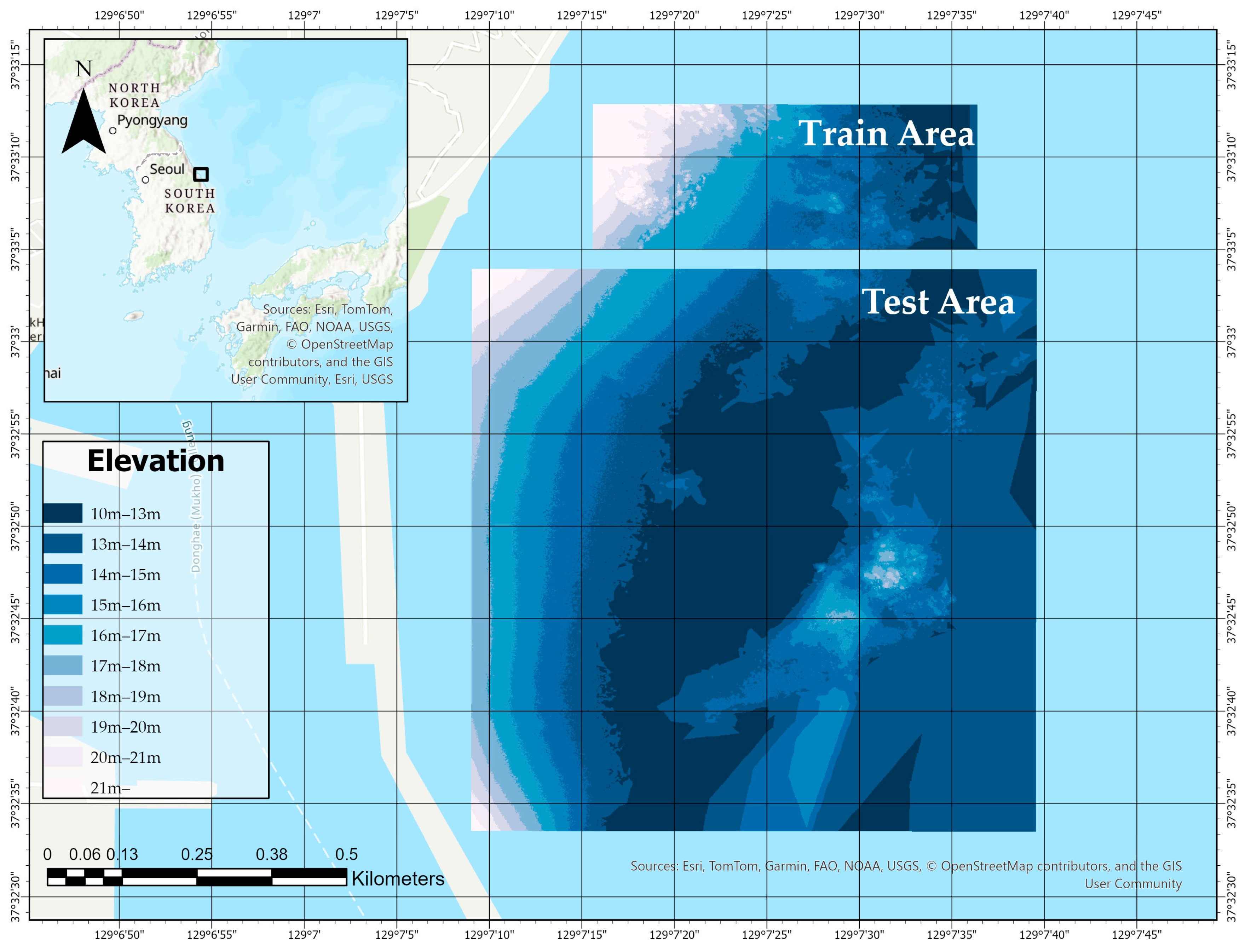
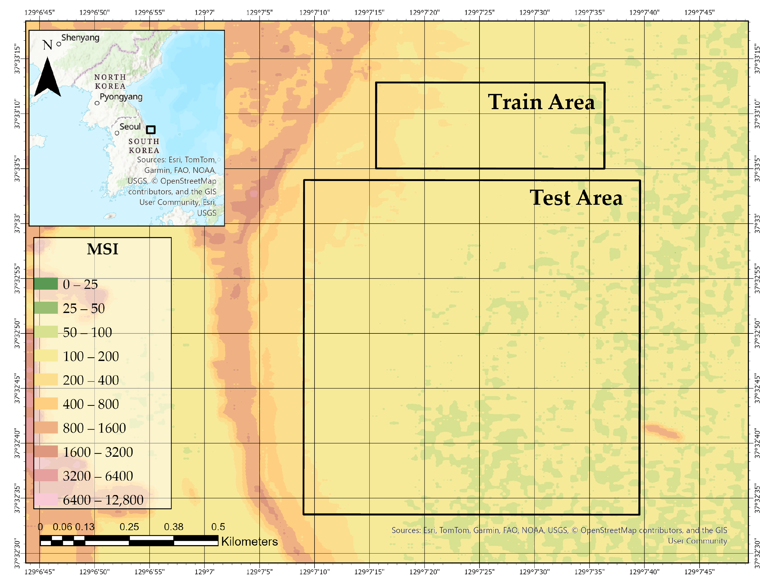
In this study, we integrate medium-resolution Sentinel-2 imagery with high-resolution bathymetric and hyperspectral reference data from the LiDAR–hyperspectral system, applying a resolution harmonization strategy in the Mukho Port area on the eastern coast of Korea (see Figure 1). To address the spatial resolution mismatch between the 10 m Sentinel-2 imagery and the 1 m LiDAR reference data, each Sentinel-2 pixel is subdivided into 100 sub-pixels, and three spatial interpolation techniques—bilinear, spline, and nearest-neighbor—are applied to upscale the spectral information.

In contrast to previous studies that adopt multitemporal stacking to reduce noise and fill temporal gaps, we did not perform stacking in this study. Instead, the use of high-resolution, co-located reference data from the airborne remote sensing platform enabled accurate spatial alignment and provided reliable ground truth for training. This allowed us to avoid the need for temporal fusion, while still ensuring spectral consistency and precise depth prediction.

The resulting upsampled datasets are then used to train Fully Connected Neural Network (FCNN) models in a pixel-wise regression framework. This approach enables a systematic evaluation of how interpolation strategies influence the accuracy of satellite-derived bathymetry (SDB), as assessed using root mean square error (RMSE) and coefficient of determination (R²) metrics.

1.5. Evaluation of Sub-Pixel Interpolation Strategies in FCNN Bathymetric Models

FCNN architectures have been shown to effectively learn complex non-linear relationships from input features, making them suitable for continuous bathymetric prediction. Prior studies [33,34] demonstrated that FCNN models using Sentinel-2 reflectance bands achieved high accuracy, with dropout and batch normalization mitigating overfitting. Additionally, ref. [20] confirmed the strong generalization capabilities of FCNNs across diverse marine optical environments.

By leveraging the high-resolution LiDAR–hyperspectral system reference datasets, the FCNN models developed in this study successfully capture fine-grained spectral–depth relationships reflecting coastal heterogeneity. Although deep learning and sensor fusion have previously been applied in SDB studies, this research uniquely contributes a systematic evaluation of sub-pixel interpolation strategies, highlighting the importance of upsampling design in optimizing model performance under varying marine optical conditions.

2. Materials and Methods

2.1. Study Area

Mukho Port, located in Donghae City along the eastern coastline of South Korea, serves as a mid-sized harbor with strategic roles in coastal logistics, fisheries, and marine tourism. The port is situated along a narrow continental shelf that descends rapidly into deeper waters, resulting in a geophysically dynamic nearshore environment. The seabed exhibits a heterogeneous composition of sand, gravel, and rock, reflecting complex geomorphological conditions. The area is subject to strong hydrodynamic forces driven by wave activity, semi-diurnal tides, and seasonally varying coastal currents, which collectively contribute to sediment resuspension and fluctuations in water clarity.

These environmental characteristics not only define the physical complexity of the Mukho region, but also introduce significant challenges for bathymetric mapping. The presence of suspended sediments, spatially variable seabed types, and fluctuating turbidity levels results in optically complex waters where traditional empirical models often underperform. To address these limitations, this study explores the application of deep learning models capable of capturing non-linear spectral–depth relationships. To support model development, high-resolution hyperspectral and bathymetric reference data were acquired using the LiDAR–hyperspectral system, while Sentinel-2 Level-2A multispectral imagery was used as the input for spectral information. These paired datasets enabled the supervised training of the proposed neural network to predict water depth from surface reflectance with enhanced robustness and generalization.

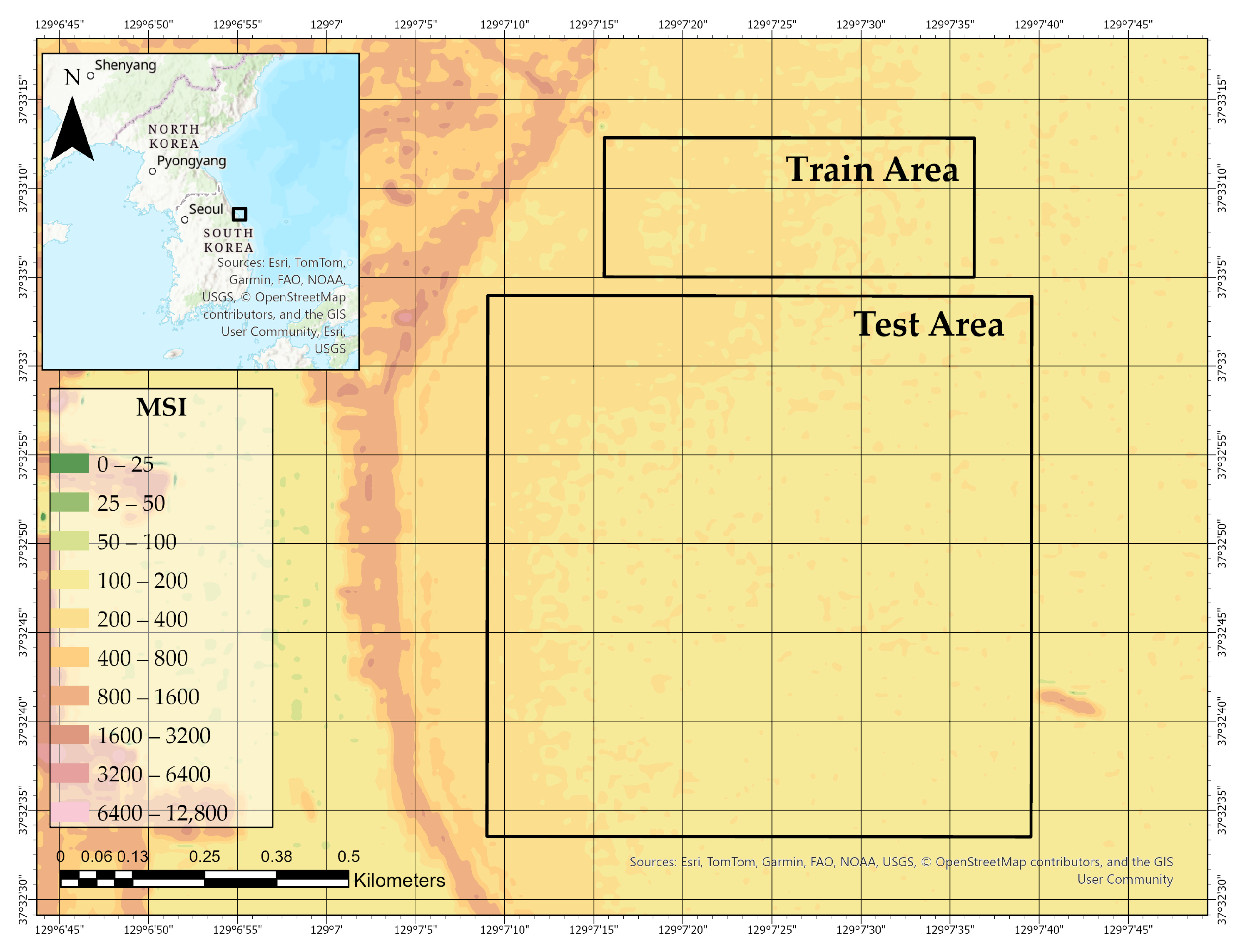
Figure 1 illustrates the spatial extent of the study site near Mukho Port on the eastern coast of South Korea and delineates two functionally distinct zones: the Train Area and the Test Area. These areas were defined based on the spatial coverage of the LiDAR–hyperspectral system datasets. The training area was used exclusively to train the bathymetric prediction models, while the test area was reserved for independent validation. This spatial separation ensures that model evaluation is conducted on unseen data, thereby minimizing spatial autocorrelation and supporting a rigorous assessment of the model’s generalization capability across heterogeneous coastal conditions. The underlying bathymetric gradient, depicted in 1 m elevation intervals, further emphasizes the geophysical complexity of the coastal environment.

2.2. Spectral and Spatial Alignment of Hyperspectral and Satellite Imagery

To effectively train the deep learning model using paired data, precise spatial and spectral alignment between the hyperspectral-derived reference bathymetry and Sentinel-2 multispectral imagery was required. The hyperspectral data obtained from the airborne remote sensing platform has a native spatial resolution of 1 m × 1 m, while Sentinel-2 Level-2A imagery has a resolution of 10 m × 10 m for its key bathymetric bands (bands 2, 3, and 4). This spatial mismatch creates challenges for pixel-wise learning in convolutional neural networks. To address this, each 10 m Sentinel-2 pixel was divided into a 10 × 10 grid of sub-pixels, generating a virtual 1 m × 1 m resolution layer. This spatial upsampling enabled alignment with the 1 m hyperspectral bathymetry data. Reflectance values for the Sentinel-2 bands (Blue: B2, Green: B3, Red: B4) were spatially interpolated to obtain sub-pixel estimates, allowing for pixel-wise pairing with the reference bathymetry.

Furthermore, to validate reflectance compatibility between the two sensors, we compared the interpolated Sentinel-2 reflectance values with co-located hyperspectral reflectance values at selected wavelengths. While the two systems differ in spectral resolution and radiometric depth (12-bit for Sentinel-2 vs. 16-bit for LiDAR–hyperspectral system), reflectance values showed consistent trends across overlapping bands, confirming suitability for paired training. Data acquisition was restricted to low-glint conditions, and Level-2A preprocessing helped mitigate atmospheric and solar reflection effects. Scenes with significant sun–sensor angle divergence were excluded to ensure radiometric comparability.

Nearest Neighbor (NN) interpolation is computationally efficient and preserves original values but may introduce blocky artifacts [35]. Spline interpolation generates smooth transitions between pixels by minimizing curvature, which can be beneficial in bathymetric gradients [36]. Inverse Distance Weighting (IDW) is widely used in geospatial applications due to its simplicity and distance-weighted averaging behavior, which can reduce edge discontinuities [37,38].

Following spatial interpolation, the resulting 1 m × 1 m Sentinel-2 reflectance layers were spatially co-registered and pixel-wise matched with the corresponding bathymetric reference values derived from hyperspectral data. This preprocessing procedure was critical for establishing a consistent input–output mapping, thereby enabling the supervised training of the Fully Connected Neural Network (FCNN) regression model.

This procedure of resolution matching and interpolation has been shown to be critical in similar SDB studies using fused or downscaled optical data [24,39]. Ensuring spatial coherence between input features and depth targets helps prevent label ambiguity during model training and improves depth estimation accuracy in optically complex waters [7,40].

2.3. Deep Learning with FCNN for Bathymetric Estimation

Recent advances in deep learning have underscored the efficacy of Fully Connected Neural Networks (FCNNs) for complex geospatial prediction tasks, particularly in coastal environments. FCNN—also known as multilayer perceptrons (MLPs)—comprise densely connected layers capable of learning non-linear relationships between spectral reflectance and water depth. In contrast to convolutional architectures that exploit spatial hierarchies, FCNNs process flattened spectral inputs, allowing them to capture intricate inter-band correlations independent of spatial adjacency. Several studies have successfully demonstrated the use of FCNNs for shallow-water bathymetry estimation from multispectral satellite data [20,33,41].

A machine learning model based on a Fully Connected Neural Network was trained to estimate shallow water depth using reflectance values from three Sentinel-2 Level-2A bands (B2, B3, and B4). As described in Section 2.2, Sentinel-2 imagery was spatially upsampled using established interpolation methods—Nearest Neighbor (NN) [42], Spline [43], and Inverse Distance Weighting (IDW) [44]—and aligned with 1 m hyperspectral-derived reference bathymetry. The reflectance inputs and corresponding bathymetric labels were aggregated into structured feature–target pairs.

Based on these paired inputs, an FCNN regression model was designed and trained as follows. The FCNN architecture consisted of an input layer, multiple hidden layers with ReLU activation functions, and a final regression output layer. Dropout and batch normalization layers were integrated to enhance model generalization and training stability [45,46]. The network was trained using a Mean Squared Error (MSE) loss function and optimized with the Adam algorithm [45]. A 20% validation split was used to monitor performance and prevent overfitting [46].

Our implementation follows a similar approach to that of [34], who demonstrated that FCNN can outperform traditional band ratio models by learning complex non-linear mappings between spectral signals and water depth. Similarly, refs. [20,41] showed that FCNNs achieve robust results across diverse optical conditions, even in turbid waters.

By leveraging high-resolution reference data and applying appropriate spatial preprocessing, this study evaluates the effectiveness of a Fully Connected Neural Network (FCNN) in modeling complex spectral–depth relationships for bathymetric estimation in optically heterogeneous coastal waters. In particular, we compare and analyze the influence of different spatial interpolation techniques—used to reconcile the resolution mismatch between hyperspectral and Sentinel-2 imagery—on the accuracy of depth prediction. This investigation, conducted within a machine learning framework, aims to assess how interpolation method selection affects model performance and generalizability, ultimately advancing scalable and accurate satellite-derived bathymetry in challenging nearshore environments.

Given the nature of the input data and the focus on pixel-level spectral relationships rather than spatial textures, we carefully considered the model architecture. While convolutional neural networks (CNNs) are widely used for image-based tasks due to their ability to extract spatial features and local patterns, our study intentionally excluded spatial-context architectures such as CNN, U-Net, and ConvLSTM. This decision was based on the nature of our input data, which comprised spectrally upsampled pixels without reliable neighborhood textures, due to the mismatch in native resolutions between Sentinel-2 (10 m) and the 1 m reference data. Our objective was to model the spectral–depth relationship at the pixel level rather than to extract spatial features across a continuous surface. Therefore, FCNN was more appropriate for treating each input vector as an independent observation without requiring spatial convolution.

The FCNN architecture was designed to capture the non-linear relationships between spectral reflectance and depth. The network consisted of an input layer with 3 nodes (for the Red, Green, and Blue bands), followed by three hidden layers: the first with 128 neurons, the second with 64 neurons, and the third with 32 neurons, all using ReLU activation functions. Dropout layers with a rate of 0.2 were added after each hidden layer to prevent overfitting and enhance model generalization. The final output layer had 1 neuron to predict water depth, with a regression output. The network was optimized using the Adam optimizer, with a learning rate of 0.001, and trained using a batch size of 100 and mean squared error (MSE) as the loss function. Early stopping was applied based on validation loss to prevent overfitting.

Given the model architecture’s capacity for non-linear regression and generalization, recent studies have demonstrated that FCNNs can effectively generalize across a wide range of hydrological and water-related conditions. For instance, ref. [47] reported that FCNNs performed as well as or better than other deep learning models in forecasting lake water levels. Similarly, refs. [48,49] showed that FCNNs successfully modeled groundwater and spring flow dynamics under diverse seasonal and climatic conditions.

2.4. Experimental Design for Interpolation Evaluation

Satellite-derived bathymetry (SDB) has traditionally relied on empirical regression models that link multispectral reflectance values to in situ depth measurements. Among these, the log-transformed band ratio model, originally proposed by [6], remains widely used due to its simplicity and effectiveness in clear waters. This model is commonly expressed as follows:

$$\mathrm{Z}={\mathrm{m}}_1·\ln \left({\displaystyle \frac{{\mathrm{R}}_{\mathrm{Blue}}}{{\mathrm{R}}_{\mathrm{Green}}}}\right)+{\mathrm{m}}_0$$

(1)

where Z is the estimated depth, R_Green and R_Blue represent the reflectance values in the green and blue bands (typically Sentinel-2 bands 3 and 2), and m₀ and m₁ are empirically fitted coefficients [6]. However, this model has significant limitations in optically complex waters due to its reliance on a linear relationship in logarithmic space and its sensitivity to factors such as water clarity, bottom type, and illumination conditions [5,7].

To address these limitations, recent studies have increasingly adopted machine learning (ML) approaches, with particular attention to Fully Connected Neural Networks (FCNNs) for their capacity to model complex, non-linear relationships between spectral reflectance and water depth. While FCNN offers robust performance in various aquatic conditions, few investigations have systematically evaluated how preprocessing steps—especially spatial interpolation techniques used to align satellite imagery with higher-resolution reference data—affect the predictive accuracy of FCNN models when operating at sub-pixel scales.

In our study, we focus on a key challenge in SDB using multispectral imagery: the spatial resolution mismatch between Sentinel-2 data (10 m) and high-resolution reference datasets such as those acquired by the airborne remote sensing platform (1 m). To address this mismatch, we performed spatial upsampling of the Sentinel-2 bands (B2, B3, B4) using three different interpolation techniques.

2.4.1. Nearest Neighbor Interpolation

Nearest Neighbor interpolation is a simple and non-parametric method that assigns to a target location the value of the nearest known sample point, without applying any smoothing or weighting. Due to its simplicity and computational efficiency, it is often used as a baseline in comparative analyses to evaluate the benefits of more advanced interpolation strategies on model training and prediction accuracy. Given a target point x₀, the interpolated value ẑ(x₀) is defined as follows [50]:

$$\widehat{\mathrm{z}}\left({\mathrm{x}}_0\right)=\mathrm{z}\left({\mathrm{x}}_{\mathrm{i}}\right),\hspace{1em}\mathrm{where}\hspace{1em}{\mathrm{x}}_{\mathrm{i}}=\arg \underset{{\mathrm{x}}_{\mathrm{j}}\in \mathrm{S}}{\min }‖{\mathrm{x}}_{\mathrm{j}}-{\mathrm{x}}_0‖$$

(2)

Here, S denotes the set of known sample points {x₁, x₂, …, x_n}, and ‖ ‖ represents the Euclidean distance. The method effectively partitions the space into Voronoi cells, with each cell assigning its central value to all points within its boundary.

Although Nearest Neighbor interpolation preserves the original data values, it introduces piecewise-constant surfaces that exhibit abrupt transitions at cell boundaries. This characteristic makes it less suitable for representing smoothly varying phenomena such as coastal bathymetry. Nonetheless, it provides a useful reference model in comparative evaluations of interpolation methods due to its minimal computational cost and absence of parameter tuning.

In the context of this study, Nearest Neighbor was implemented as one of the three upsampling strategies to interpolate Sentinel-2 pixel reflectance from 10 m to 1 m resolution. The results were used to assess its effect on the accuracy and spatial continuity of satellite-derived bathymetry (SDB) when compared with more advanced techniques such as bilinear and spline interpolation.

2.4.2. Spline Interpolation

Spline interpolation constructs a smooth, continuous surface by fitting low-degree polynomials to local subsets of the data. In two-dimensional spatial interpolation, bicubic splines are commonly used due to their ability to model both gradual transitions and subtle curvature without introducing oscillations. This makes the method particularly suitable for upsampling satellite reflectance imagery where spectral gradients vary smoothly across coastal waters.

Given a grid of known pixel values z(x_i, y_j), bicubic spline interpolation estimates the value at a target location (x₀, y₀) by combining a weighted sum of the surrounding 16 neighboring points using a third-order polynomial basis [51], as follows:

$$\widehat{\mathrm{z}}\left({\mathrm{x}}_0,{\mathrm{y}}_0\right)=\sum _{\mathrm{i}=0}^3\sum _{\mathrm{j}=0}^3{\mathrm{a}}_{\mathrm{i}\mathrm{j}}·{\left({\mathrm{x}}_0-\mathrm{x}\right)}^{\mathrm{i}}·{\left({\mathrm{y}}_0-\mathrm{y}\right)}^{\mathrm{j}}$$

(3)

where a_ij are spline coefficients determined by matching function values and derivatives at grid boundaries. The spline formulation ensures continuity up to the second derivative, resulting in a surface that is smooth in both gradient and curvature.

In this study, bicubic spline interpolation was applied to resample Sentinel-2 imagery from its native 10 m resolution to 1 m sub-pixel grids. This process preserves fine-scale spectral variation essential for learning depth-sensitive features in Fully Connected Neural Network (FCNN) models. The smooth transition between pixels helps minimize spectral discontinuities introduced by other interpolation methods, improving model stability and predictive accuracy in optically heterogeneous coastal zones.

2.4.3. Inverse Distance Weighting (IDW) Interpolation

Inverse Distance Weighting (IDW) is a deterministic spatial interpolation technique that estimates unknown values at unsampled locations by calculating a weighted average of neighboring observations, with weights assigned inversely proportional to the distance between points.

Given a set of known sample points {x₁, x₂, …, x_n} with associated values {z(x₁), z(x₂), …, z(x_n)}, the interpolated value ẑ(x₀) at an unsampled location x₀ is computed as follows [52]:

$$\widehat{\mathrm{z}}\left({\mathrm{x}}_0\right)={\displaystyle \frac{{\sum }_{\mathrm{i}=1}^{\mathrm{n}}{\mathrm{w}}_{\mathrm{i}}·\mathrm{z}\left({\mathrm{x}}_{\mathrm{i}}\right)}{{\sum }_{\mathrm{i}=1}^{\mathrm{n}}{\mathrm{w}}_{\mathrm{i}}}}\hspace{1em}\mathrm{where}\hspace{1em}{\mathrm{w}}_{\mathrm{i}}={\displaystyle \frac{1}{\mathrm{d}{\left({\mathrm{x}}_0,{\mathrm{x}}_{\mathrm{i}}\right)}^{\mathrm{p}}}}$$

(4)

Here, d(x₀, x_i) represents the Euclidean distance between the target location x₀ and the i-th known point x_i, and p is a user-defined power parameter that controls the influence of distance on the weights. A higher value of p increases the influence of nearer points and decreases the impact of distant ones, typically with p ∈ [1, 3].

IDW offers several advantages in satellite-derived bathymetry (SDB) preprocessing. It is computationally efficient, easy to implement, and adapts well to irregularly spaced datasets. However, it does not guarantee surface smoothness and may produce artifacts near data clusters or boundaries if not properly parameterized. Nonetheless, when combined with high-resolution reference data, IDW provides a robust means of spatial upsampling for training pixel-wise learning models such as FCNNs in coastal optical environments.

By holding the FCNN architecture and training configuration constant across all experiments, we isolate the interpolation method as the sole variable. This design allows us to evaluate how input preprocessing affects model learning and prediction performance. The FCNN model was trained on over 100,000 paired pixels and validated against a reserved test set from the Mukho Port region, an optically diverse nearshore area characterized by sandy and rocky seabeds, variable turbidity, and bathymetric gradients.

2.5. Model Validation and Accuracy Assessment

To evaluate the performance of the proposed bathymetric estimation models, a validation framework was established to assess the influence of input spectral configuration and interpolation strategy on predictive accuracy. Two types of spectral inputs were tested: (1) the commonly used logarithmic band ratio ln(B2/B3), frequently employed in satellite-derived bathymetry (SDB) studies due to its empirical correlation with water depth, and (2) raw reflectance values from Sentinel-2 Bands 2, 3, and 4 (i.e., RGB), offering a physically interpretable input representation derived from multispectral imagery.

For each input configuration, the predicted bathymetric raster was validated against high-resolution LiDAR-derived depth data, which served as the ground truth. Prior to evaluation, the predicted outputs were spatially aligned with the LiDAR reference through reprojection and resampling to ensure consistent resolution (1 m), spatial extent, and coordinate system. Only pixels with valid (non-missing) values in both datasets were included in the analysis to eliminate the effects of data voids or boundary artifacts.

Prediction accuracy was quantified using four standard statistical metrics: Root Mean Square Error (RMSE), Mean Absolute Error (MAE), coefficient of determination (R²), and mean bias. These metrics jointly capture the overall error magnitude, average deviation, explanatory power, and directional bias of predictions. By applying a consistent and reproducible evaluation procedure across all model configurations, this assessment enables a robust comparison of model performance under varying input and preprocessing scenarios.

The validated results and associated accuracy statistics are reported and analyzed in Section 3.

2.6. Workflow of FCNN-Based Bathymetric Estimation Using Interpolated Sentinel-2 Imagery

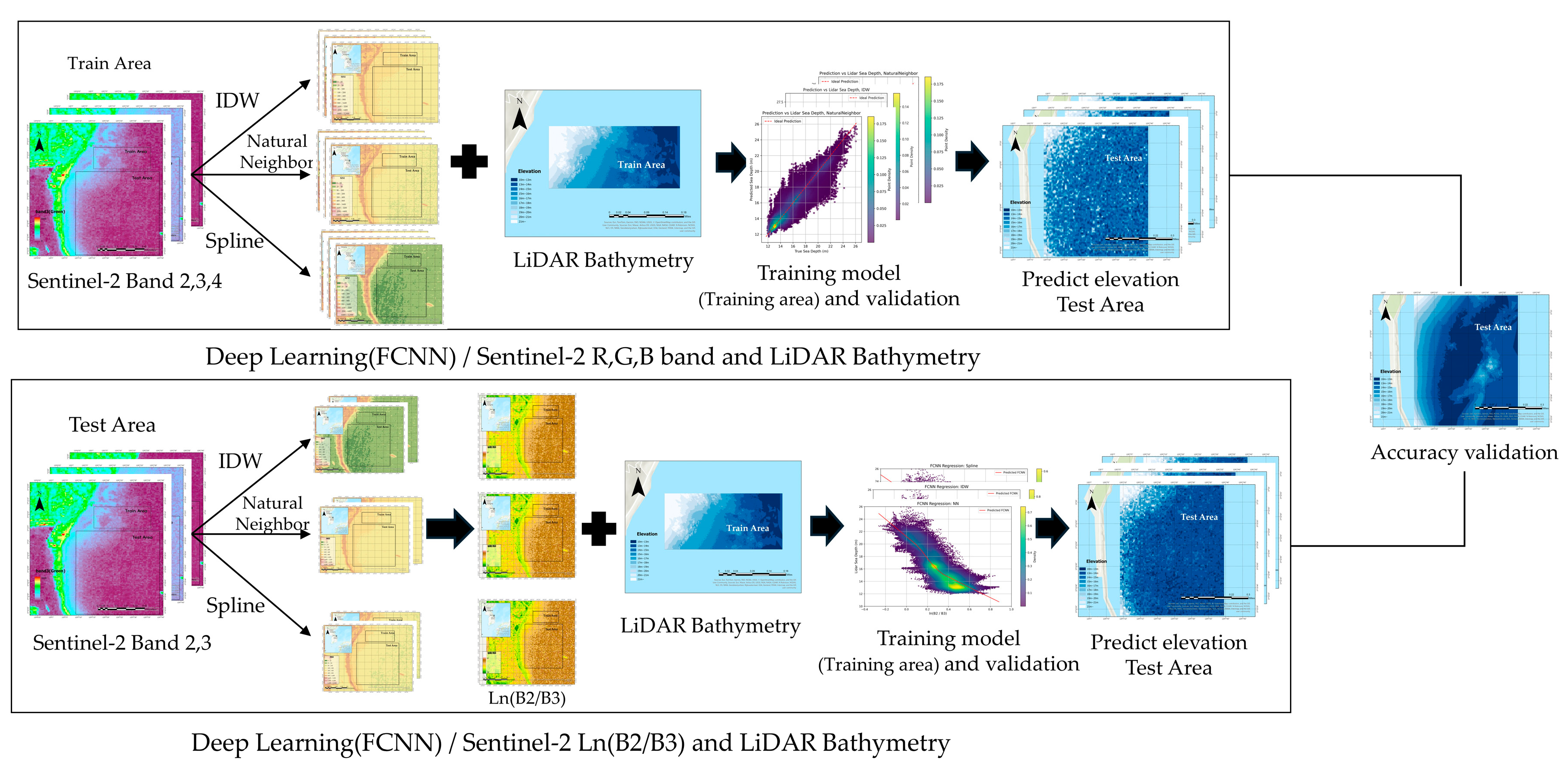
This study presents a deep learning-based framework for estimating shallow water bathymetry using Sentinel-2 multispectral imagery and high-resolution LiDAR-derived reference data. The complete experimental workflow is illustrated in Figure 2.

Three visible bands from Sentinel-2—Band 2 (blue), Band 3 (green), and Band 4 (red)—were utilized due to their proven effectiveness in aquatic remote sensing applications. To reconcile the spatial resolution mismatch between 10 m Sentinel-2 imagery and 1 m LiDAR-derived bathymetric data, three commonly adopted spatial interpolation methods—Inverse Distance Weighting (IDW), Natural Neighbor, and Spline—were applied to the spectral bands.

Two distinct input configurations were designed for bathymetric model training and prediction, as illustrated in Figure 2:

(a)

This approach utilizes the raw reflectance values from the Sentinel-2 red, green, and blue bands (Bands 4, 3, and 2, respectively) as input features, and trains a Fully Connected Neural Network (FCNN) using LiDAR-derived bathymetric data as ground truth. For each band, three spatial interpolation techniques—Inverse Distance Weighting (IDW), Natural Neighbor, and Spline—were applied to upscale the imagery from 10 m to 1 m resolution. The interpolated spectral bands were spatially aligned with the LiDAR bathymetry to form pixel-wise training pairs. The FCNN was trained and validated on this dataset and subsequently applied to predict elevation values in a separate test area using Sentinel-2 reflectance data processed with the same interpolation methods.

(b)

This approach computes the natural logarithmic ratio ln(B2/B3) from the Sentinel-2 blue (Band 2) and green (Band 3) bands, and uses this ratio as the input feature to train the FCNN with LiDAR-derived bathymetry as the target variable. The log-ratio images were generated over the test area and interpolated to 1 m resolution using the same three spatial methods. These were then spatially registered with the LiDAR bathymetry of the training area to create the learning dataset. The trained FCNN was then applied to the log-ratio images from the test area, which had been processed identically, to predict elevation values.

The RGB reflectance configuration exploits spectral variation across bands to infer bathymetry but is susceptible to noise from surface glint, turbidity, and bottom reflectance. In contrast, the ln(B2/B3) ratio captures wavelength-dependent attenuation, often yielding a more monotonic and depth-correlated signal in optically shallow waters. This transformation is widely adopted in analytical SDB models for its ability to suppress surface noise and enhance depth-related spectral gradients.

Both configurations employed the same FCNN architecture, consisting of three fully connected hidden layers with ReLU activation functions and a single output node for continuous depth prediction. The network was trained using the mean squared error (MSE) loss function to model the non-linear relationship between the spectral inputs and LiDAR-derived depths.

In both configurations, the FCNN architecture remained consistent, composed of multiple densely connected layers. The models were trained using the Mean Squared Error (MSE) loss function and optimized via the Adam optimizer. Model performance was evaluated using Root Mean Square Error (RMSE) and the coefficient of determination (R²), comparing predicted depths with reference LiDAR data.

This comparative framework enabled a systematic analysis of how input feature types and interpolation techniques affect the accuracy of satellite-derived bathymetric estimates, thereby identifying optimal preprocessing strategies for remote sensing-based mapping in optically complex nearshore environments.

3. Results

3.1. Spatial Configuration of Training and Testing Areas with Reference Data for FCNN

To construct and evaluate the Fully Connected Neural Network (FCNN) model, the study region was spatially divided into two independent areas: a training area and a testing area. This division was designed to ensure a clear separation between model development and validation, thereby minimizing spatial information leakage.

The training area was selected to encompass diverse terrain characteristics and elevation variability that are representative of the broader geographical context. High-resolution elevation data were used as both input features and ground truth references for model learning. This area provided the basis for supervised training, enabling the FCNN to learn spatial patterns and elevation-related features relevant to the application domain.

The precise extent and distribution of the training region are illustrated in Figure 1 (Section 2.1).

The training dataset was derived from airborne remote sensing conducted in August 2020, using the airborne remote sensing platform, a state-of-the-art dual-sensor platform capable of collecting both topographic and bathymetric LiDAR data alongside high-resolution hyperspectral imagery. This system captured detailed surface characteristics across the training region, providing elevation estimates with high spatial accuracy.

In particular, the hyperspectral sensor onboard the LiDAR–hyperspectral system collected reflectance data across 421 spectral bands (used 58 bands), enabling enhanced differentiation of land surface materials and conditions. When fused with LiDAR-derived elevation measurements, these data formed a rich and reliable training set that facilitated supervised learning of spatial and spectral elevation patterns by the FCNN.

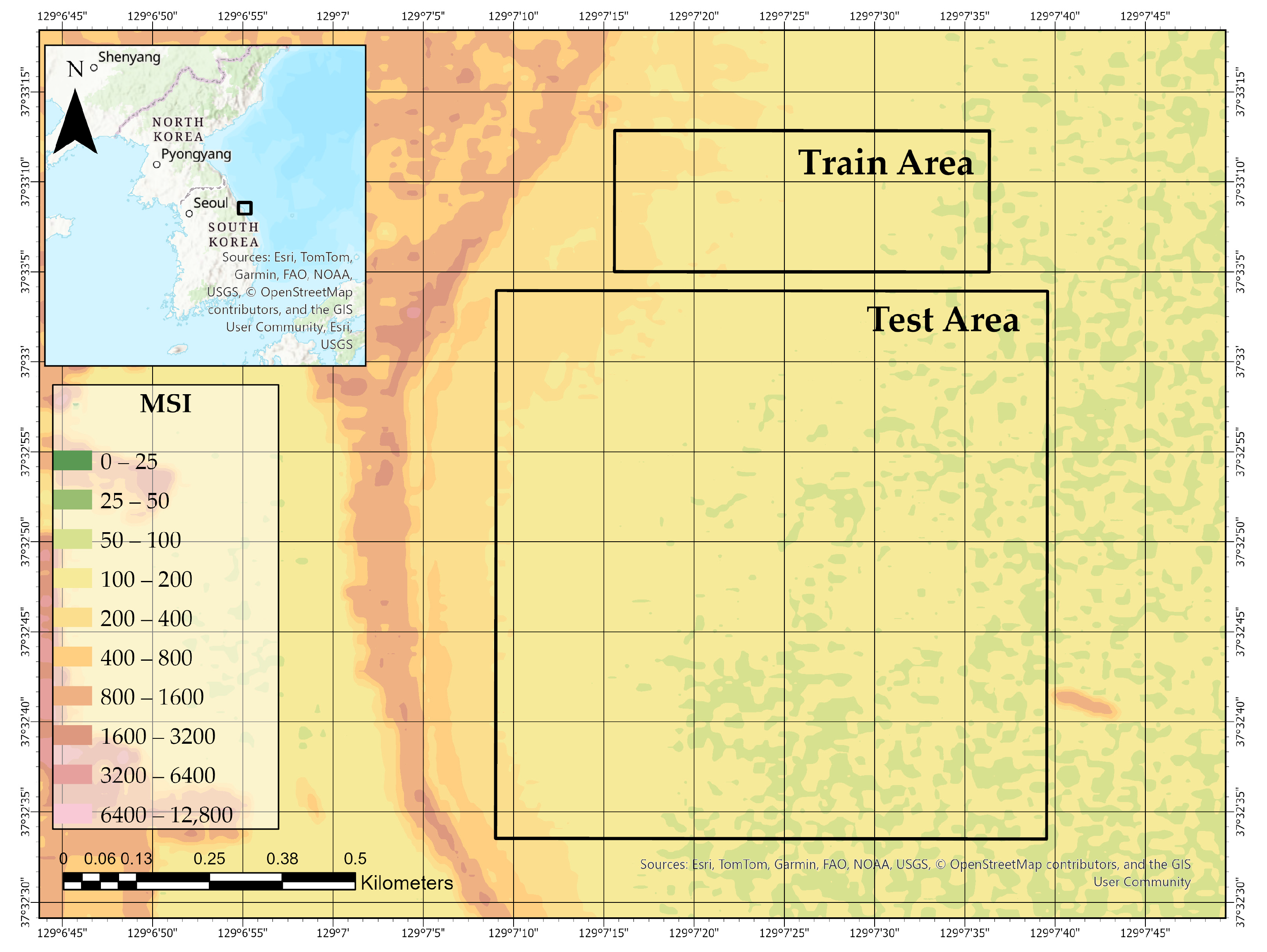
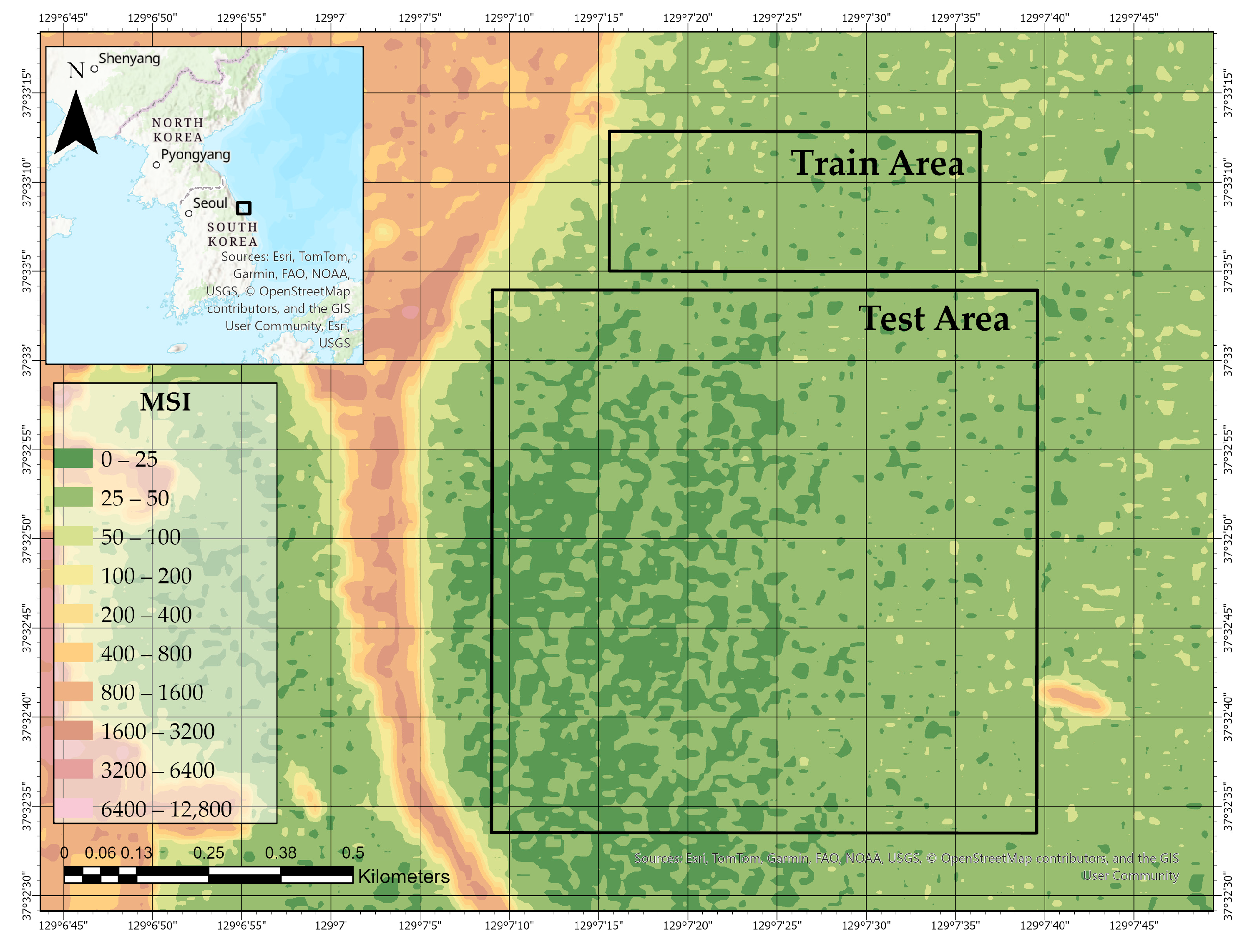
To assess the model’s generalization capability, a geographically independent testing area was designated and excluded entirely from the training process. As illustrated in Figure 3 this region is located along a separate coastal zone and exhibits different elevation characteristics compared to the training area.

The testing dataset was also acquired using the airborne remote sensing platform during the same airborne survey conducted in August 2020, ensuring consistency in spatial resolution and spectral quality across both regions. By maintaining identical sensor configurations and acquisition conditions, the test area provides a reliable basis for evaluating the ability of FCNN to predict elevation from hyperspectral inputs under unseen spatial conditions.

This experimental design ensures that the performance evaluation reflects true model generalization, rather than memorization of spatially correlated patterns from the training data.

3.2. Interpolation-Based Resampling of Sentinel-2 Bands for High-Resolution Bathymetric Modeling

To address the resolution mismatch between Sentinel-2 imagery (10 m) and the 1 m airborne bathymetric reference data, Sentinel-2 bands were upsampled to 1 m using three interpolation methods: Inverse Distance Weighting (IDW, power = 2), Nearest Neighbor (NN), and regularized Spline (order = 3). All processes were performed in ArcGIS Pro 3.5 to maintain geospatial consistency. The resulting 1 m reflectance layers were then used as inputs for pixel-wise FCNN training.

3.2.1. Natural Neighbor Interpolation for Sentinel-2 Band Resampling

To improve spatial consistency between Sentinel-2 reflectance data and high-resolution bathymetric references, we applied Natural Neighbor interpolation to resample the multispectral imagery from its original 10 m resolution to a 1 m grid. This geometric, non-parametric interpolation technique is based on Voronoi tessellation and does not require any user-defined parameters, making it well-suited for spatially adaptive resampling.

Natural Neighbor interpolation offers several advantages:

• It provides exact interpolation at known data points;
• Produces smooth transitions and natural boundaries without overshoot;
• Adapts robustly to irregular point distributions without explicit tuning.

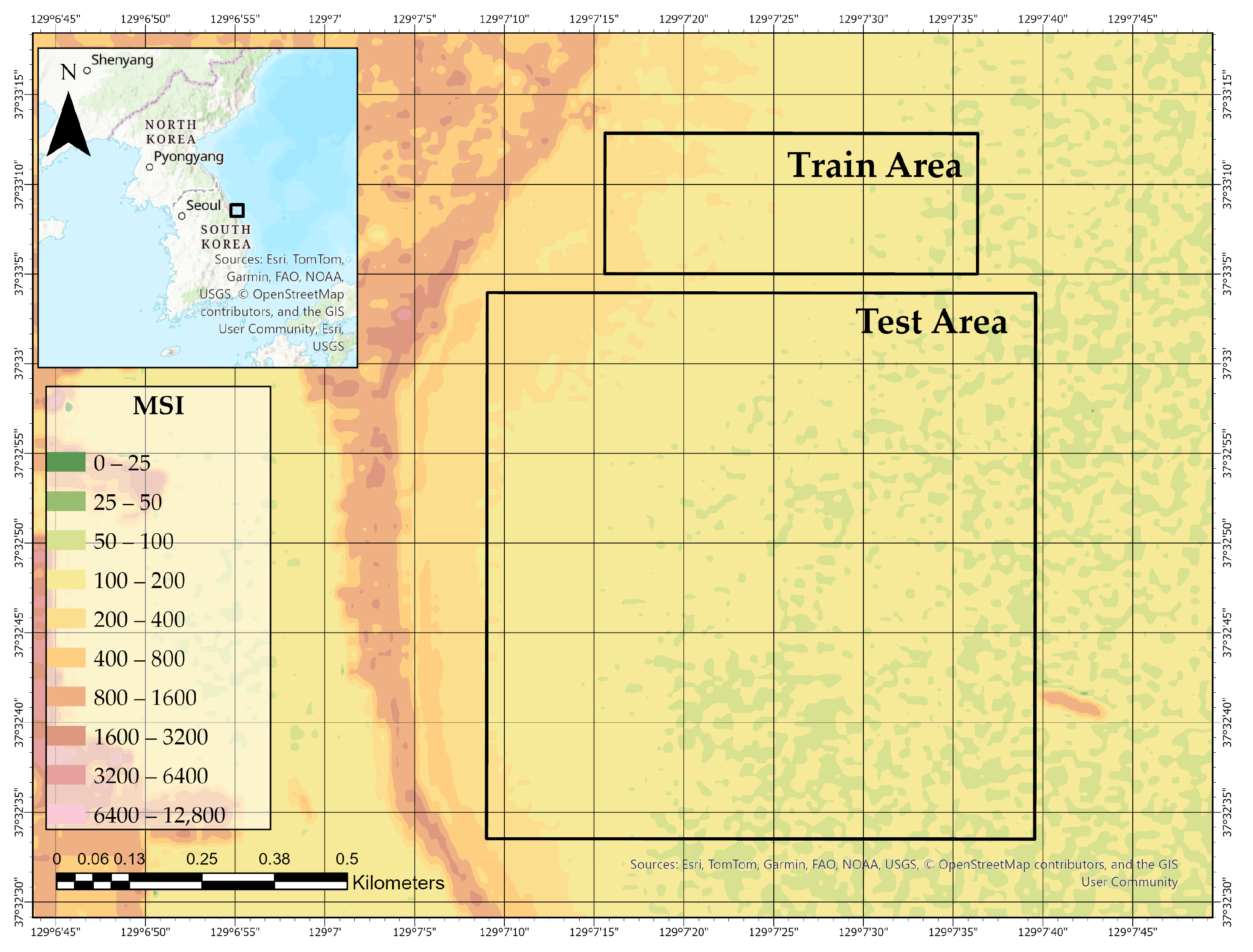
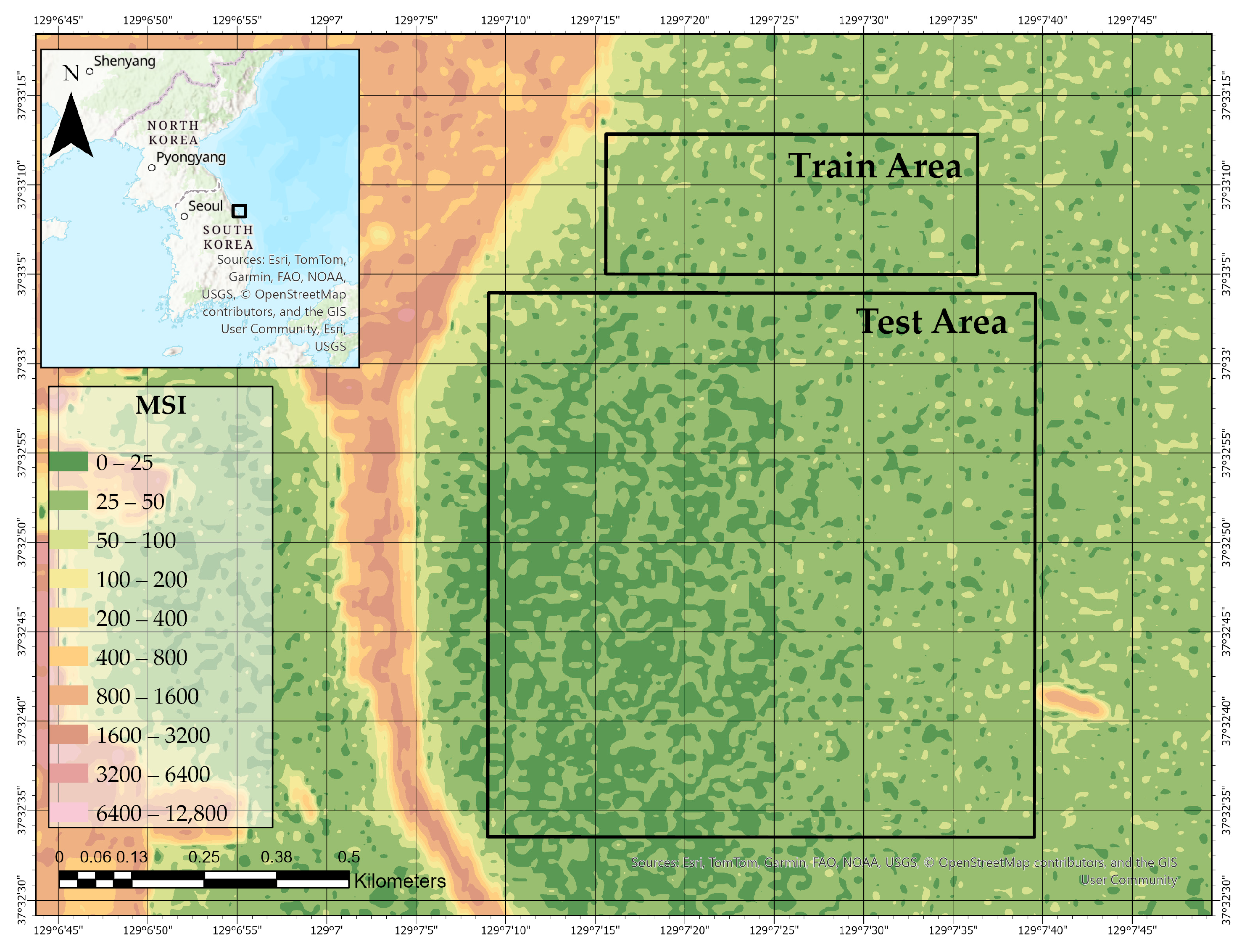
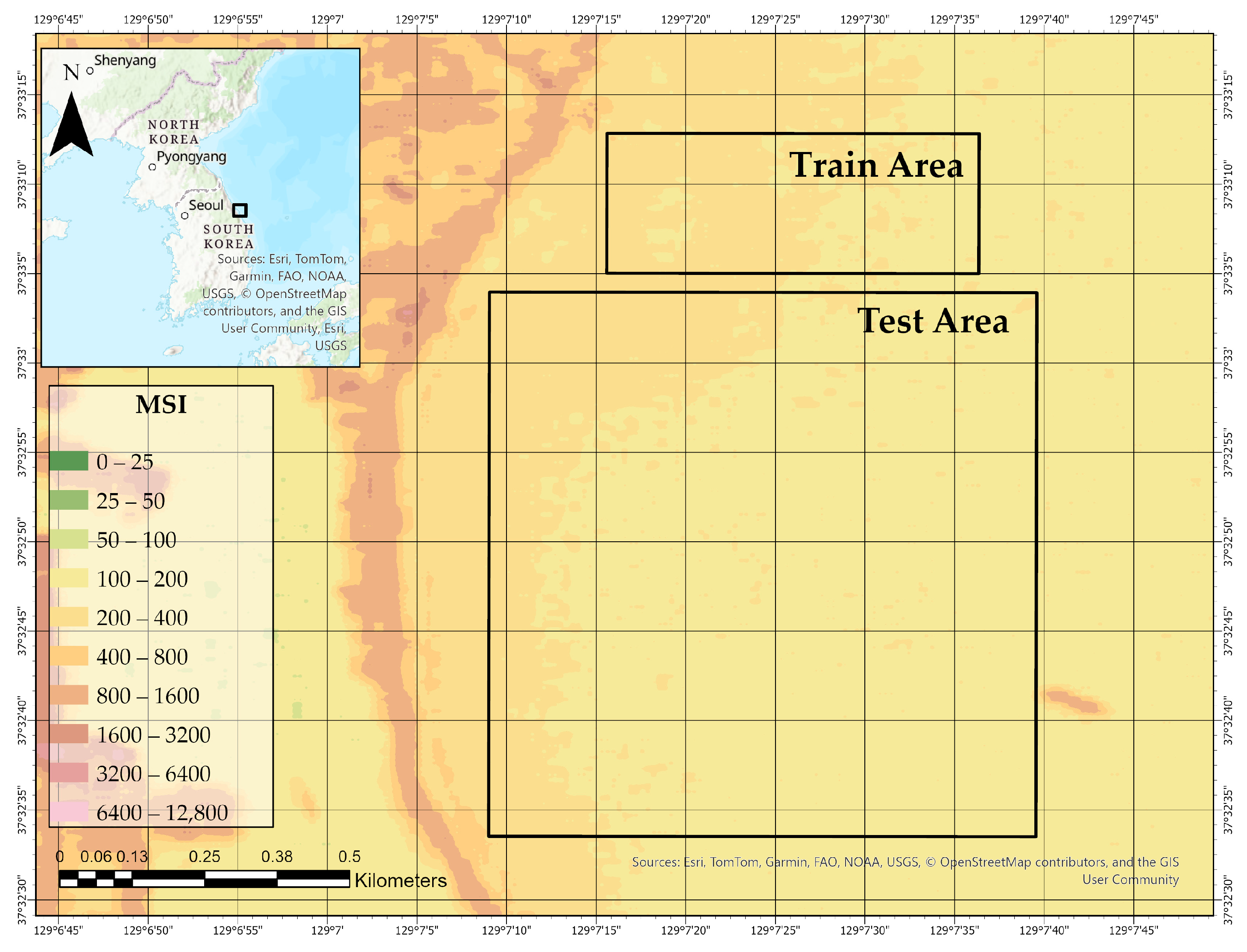
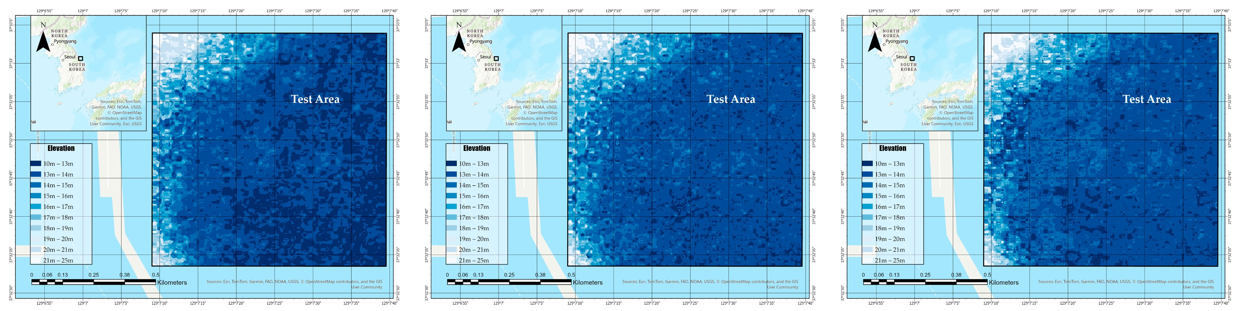
In our implementation, Band 2 (Blue), Band 3 (Green), and Band 4 (Red) of the Sentinel-2 MSI were individually resampled using this method. The results are presented in Figure 3, Figure 4 and Figure 5, showing the spatial distribution of reflectance across the Train and Test Areas.

3.2.2. Spline Interpolation for Sentinel-2 Band Resampling

To complement the geometric-based approach, this study also applied spline interpolation for generating spatially continuous and visually smooth reflectance surfaces from Sentinel-2 imagery. Spline interpolation is a well-established mathematical technique that constructs piecewise polynomial functions between known data points, ensuring local smoothness while minimizing abrupt transitions.

This structure guarantees that the resulting interpolation minimizes curvature while maintaining smooth transitions across the raster surface.

In this study, Band 2 (Blue), Band 3 (Green), and Band 4 (Red) of the Sentinel-2 MSI data were each independently resampled from 10 m to 1 m resolution using the cubic spline method. The resampled rasters were aligned spatially with the airborne LiDAR bathymetric grid, enabling consistent input preparation for subsequent model training. The results are presented in Figure 6, Figure 7 and Figure 8, showing the spatial distribution of reflectance across the Train and Test Areas.

3.2.3. Inverse Distance Weighting (IDW) for Sentinel-2 Band Resampling

Key advantages of spline interpolation include its numerical stability, minimal risk of overfitting, and smooth representation of continuous gradients, which are particularly beneficial when modeling natural surfaces such as seabed morphology. By leveraging localized polynomial fitting, spline interpolation provides a flexible yet robust means of resampling multispectral satellite data for high-resolution geospatial applications.

To ensure pixel-wise spatial consistency between Sentinel-2 reflectance imagery and airborne LiDAR bathymetric data, each visible band—Band 2 (Blue), Band 3 (Green), and Band 4 (Red)—was individually resampled to a 1 m resolution grid using the Inverse Distance Weighting (IDW) interpolation method. The study area encompassed the coastal region of Mukho Port, where fine-scale resampling was critical for accurate depth estimation and geospatial alignment.

Each Sentinel-2 band was interpolated independently using this method. The resulting reflectance surfaces ensured a smooth and continuous spatial structure suitable for direct integration with LiDAR-derived bathymetric data in the modeling workflow. The results are presented in Figure 9, Figure 10 and Figure 11, showing the spatial distribution of reflectance across the Train and Test Areas

3.2.4. Comparative Analysis of Interpolation Methods via Deep Learning-Based Bathymetry

This study investigated how different interpolation techniques used during the preprocessing of Sentinel-2 imagery influence the performance of satellite-derived bathymetry (SDB) when applied to deep learning models. Specifically, three interpolation methods—Inverse Distance Weighting (IDW), Natural Neighbor, and Spline interpolation—were used to resample the 10 m resolution reflectance data to a 1 m resolution, enabling pixel-level alignment with airborne LiDAR bathymetric reference data.

Each method offers distinct characteristics:

• Natural Neighbor interpolation provides strong local adaptability and produces smooth, continuous surfaces without requiring parameter tuning. Its geometric basis ensures robustness in areas with irregular sample distributions and sharp terrain transitions.
• Spline interpolation utilizes piecewise polynomial functions to create smooth gradients with minimal curvature distortion. This method is particularly effective for modeling gradual and continuous changes in natural surfaces such as seabeds.
• IDW interpolation is computationally efficient and easy to implement, relying on distance-weighted averaging. While more sensitive to the spatial distribution of input data, it offers a practical trade-off between simplicity and performance.

To assess the impact of these interpolation strategies on bathymetric modeling, a Fully Convolutional Neural Network (FCNN) was trained using the resampled datasets under two different spectral input configurations:

• Log-ratio input model: Utilizes the natural logarithm of the band ratio, ln(B2/B3), a known spectral indicator of water depth.
• RGB composite input model: Incorporates raw reflectance values from Sentinel-2 Bands 2 (Blue), 3 (Green), and 4 (Red) as a multi-channel input.

For each interpolation method, the FCNN was trained with the same architecture and input configuration to predict LiDAR-based seabed depth over the test area. This allowed for direct comparisons in predictive performance.

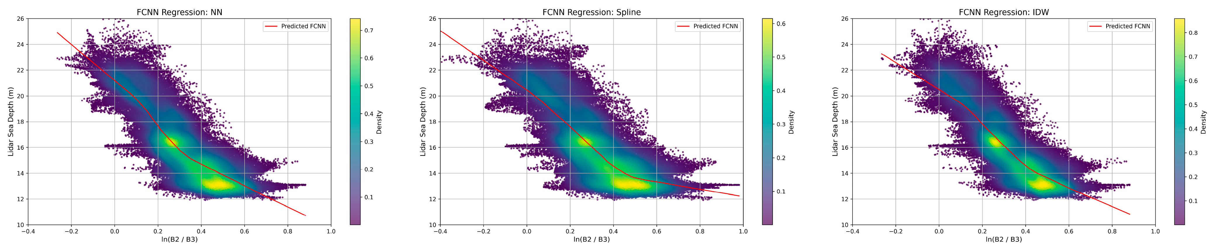
To visualize the impact of each interpolation method on the model’s predictive behavior, the relationships between the logarithmic spectral input, ln(B2/B3), and the corresponding LiDAR-derived depths were plotted, overlaid with the FCNN-predicted regression curves. Figure 12 illustrates the prediction trends learned by the network across the three interpolation cases—Natural Neighbor, Spline, and IDW—based on the test dataset.

Each subplot illustrates the relationship between the logarithmic band ratio ln(B2/B3) and the corresponding LiDAR-derived seabed depths, visualized as a two-dimensional density distribution. Warmer colors indicate areas with higher point concentration, and the red curve denotes the mean predicted depth by the Fully Connected Neural Network (FCNN) across the spectral gradient.

In the Natural Neighbor (NN) case, the regression curve exhibits a smooth and continuous transition, effectively capturing the local variations in the spectral-depth relationship. The high-density region is clearly delineated, reflecting the method’s robustness in preserving spatial detail and adapting to localized input characteristics.

The Spline interpolation result reveals a regression curve with more pronounced curvature and localized fluctuations. While the spline method maintains continuity, it may introduce sensitivity to gradient transitions, particularly in regions with abrupt changes in seabed morphology.

In contrast, the IDW-based input yields a relatively flatter and smoother regression curve. Although this method ensures computational efficiency, the model response appears more generalized, potentially due to the averaging effect inherent in distance-weighted interpolation, especially in areas with uneven sample distributions.

These results demonstrate that the spatial structure induced by the choice of interpolation method can significantly influence the learned spectral-depth response of the network, thereby affecting the accuracy and reliability of satellite-derived bathymetry predictions.

3.3. Spatial Visualization of FCNN Bathymetric Predictions by the Interpolation Method

To complement the regression-based evaluation of spectral input and interpolation methods, this section presents a spatial analysis of the predicted bathymetry produced by the Fully Convolutional Neural Network (FCNN). While prior sections focused on the spectral-depth relationship using aggregated data points, it is equally important to assess the geospatial consistency and surface morphology reflected in the model’s outputs.

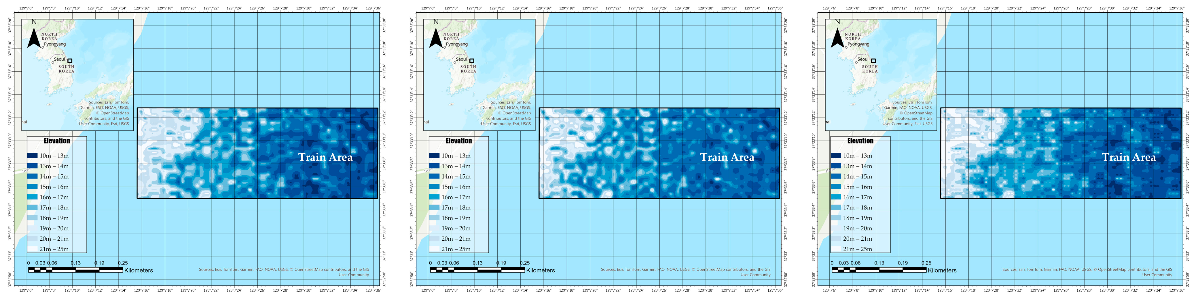
Figure 13 illustrates the spatial distribution of predicted bathymetric depth over the training area for three different interpolation methods—Natural Neighbor, Spline, and IDW—using ln(B2/B3) as the sole input feature. Each map was generated using identical FCNN architecture and training parameters, ensuring that variations in the resulting elevation surfaces are attributable solely to differences in input resampling.

The purpose of this comparison is to evaluate the impact of interpolation choice on spatial continuity, artifact presence, and the preservation of fine-scale bathymetric features. Such visual inspection provides insight into the practical implications of preprocessing choices, particularly when FCNNs are deployed for pixel-level seabed depth estimation in operational settings.

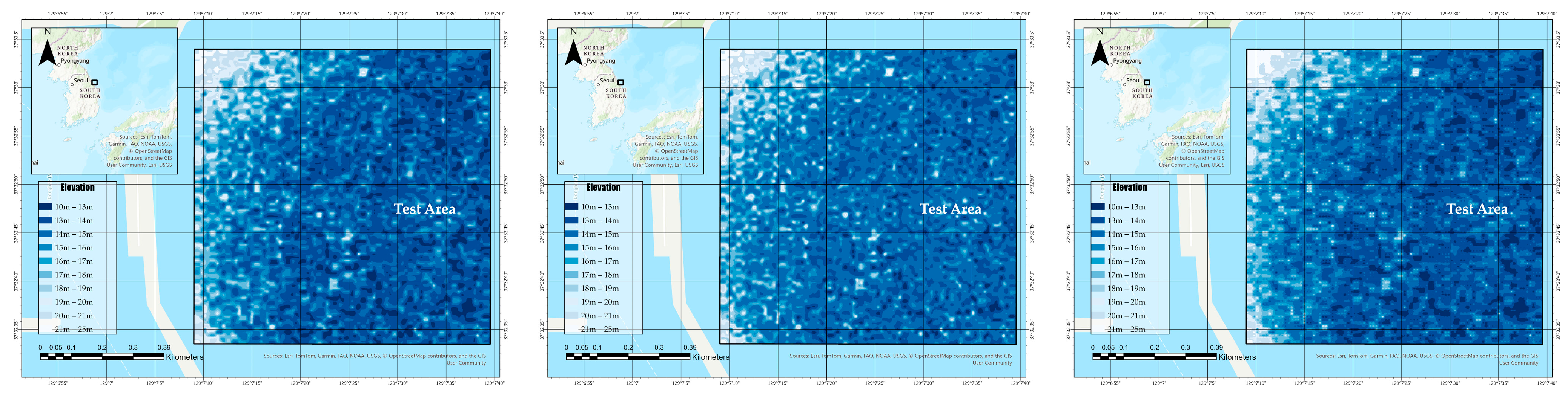
To assess the spatial generalizability of the FCNN-based bathymetric prediction models beyond the training extent, this section presents the predicted elevation surfaces over the designated test area. Using the same log-ratio spectral input configuration (ln(B2/B3)), FCNN models trained with input reflectance data interpolated by Natural Neighbor, Spline, and IDW methods were applied to unseen regions. Figure 14 provides a visual comparison of the resulting bathymetric maps generated by each model under identical inference conditions.

Figure 13 presents the predicted bathymetric surfaces over the test area using FCNN models trained with reflectance inputs interpolated via Natural Neighbor, Spline, and IDW methods. All models received the same log-ratio input (ln(B2/B3)) and were applied under identical inference settings, ensuring that the observed spatial differences reflect only the influence of the interpolation technique used during preprocessing.

The Natural Neighbor-based prediction maintains a smooth and continuous bathymetric gradient, effectively preserving coastal contours and local variations. In contrast, the Spline interpolation result exhibits greater localized fluctuation, especially along transition zones, which may indicate sensitivity to gradient irregularities. The IDW-based output appears more blocky and less coherent in terms of fine-scale structure, suggesting a potential loss of spatial detail due to oversmoothing.

These results highlight the role of input resampling in shaping the model’s generalization performance. In operational applications where models are deployed over unseen regions, such preprocessing choices can significantly impact the consistency and reliability of the predicted seabed morphology.

3.4. RGB-Based Bathymetric Prediction Under Different Interpolation Schemes

To complement the log-ratio analysis presented in the previous sections, this part investigates the spatial prediction performance of FCNN models trained with raw reflectance values from Sentinel-2 Bands 2 (Blue), 3 (Green), and 4 (Red) as a three-channel input. While the log-ratio is a widely used depth indicator, using RGB composites allows the network to learn multi-band interactions directly from reflectance data without predefined spectral transformations.

Figure 15 displays the bathymetric prediction maps generated over the training area using FCNNs trained with reflectance inputs resampled via three interpolation techniques: Natural Neighbor, Spline, and IDW. As in prior experiments, the network architecture and training configuration were kept constant, enabling direct comparison of the spatial effects induced by each interpolation method.

This analysis aims to evaluate how the use of raw multi-band input influences the sensitivity of FCNN models to input surface structure, and how interpolation strategies affect the network’s ability to reconstruct fine-scale bathymetric features within the training region.

To assess the extrapolation capability of RGB-based bathymetric models, Figure 16 presents the predicted elevation maps over the test area using FCNNs trained with three-band Sentinel-2 reflectance input. As in the training phase, the input data were resampled using Natural Neighbor, Spline, and IDW interpolation methods. By applying the same network architecture and inference settings, this evaluation isolates the influence of the interpolation strategy on the model’s ability to generalize bathymetric patterns beyond the training domain.

This comparison provides insight into how spatial smoothing, feature distortion, and resolution degradation manifest when RGB composites are used as input, highlighting the practical considerations of using raw reflectance bands for depth estimation in operational coastal mapping.

Figure 16 displays the bathymetric prediction results over the test area using FCNN models trained with raw RGB reflectance input and three different interpolation methods applied during preprocessing. While the overall bathymetric gradients are captured consistently across all three maps, notable differences are observed in spatial detail, noise levels, and edge continuity.

The Natural Neighbor result shows a relatively smooth transition from shallow to deep areas, maintaining spatial coherence with minimal artifacts. The Spline-based prediction exhibits more irregularities and local undulations, which may result from oversensitivity to small variations in interpolated input values. In contrast, the IDW result tends to produce blocky patterns and a coarser appearance, indicating potential loss of fine-scale seabed morphology due to the averaging nature of the method.

These observations underscore that the choice of interpolation method not only affects the fidelity of training inputs, but also has a lasting influence on the model’s generalization performance. When RGB inputs are used without spectral transformation, the quality and spatial consistency of the reflectance surface become even more critical to achieving reliable depth predictions in unseen areas.

3.5. Schemes Comparative Evaluation of Bathymetric Prediction Accuracy Using Log-Ratio and RGB Inputs

To assess the influence of input spectral configuration and interpolation strategies on model performance, this section presents a comparative evaluation of bathymetric prediction accuracy using two types of inputs: the commonly used log-ratio feature ln(B2/B3) and raw reflectance values from Sentinel-2 Bands 2, 3, and 4 (RGB).

Overall, the model trained with RGB input outperformed the log-ratio-based model across multiple quantitative metrics. First, the RGB-based FCNN demonstrated lower prediction errors, with reduced RMSE and MAE values, indicating improved precision. Second, the mean prediction bias—reflecting the difference between the predicted and true depth means—was significantly smaller in the RGB model, suggesting that predictions were more directionally aligned with reference values. Third, the coefficient of determination (R²) was consistently higher for the RGB input, implying better explanatory power in capturing depth variance.

Further performance differentiation was observed depending on the interpolation or regression scheme applied to the input data. Among all tested configurations, the model using Nearest Neighbor interpolation with RGB input yielded the best results. Specifically, it achieved the lowest RMSE of 1.2320 m, the lowest MAE of 0.9381 m, and the highest R² of 0.6261, indicating both accuracy and robustness. Moreover, the prediction bias was +0.0315, which is effectively negligible, indicating near-unbiased estimation.

These results suggest that RGB bands retain more raw spectral information than log-ratio transformations, providing a richer input space for the network to learn depth-related features. In addition, locally adaptive methods such as Nearest Neighbor interpolation may better preserve spatial continuity and topographic transitions in the seabed, enhancing predictive reliability.

Therefore, for bathymetric modeling in coastal environments similar to the study site, using raw RGB inputs in combination with locally sensitive interpolation techniques—particularly Nearest Neighbor—may constitute an optimal approach.

Finally, the quantitative results comparing prediction accuracy across different input types and interpolation methods are summarized in

Table 1. Quantitative performance metrics of FCNN-based bathymetric prediction models using different combinations of input type (log-ratio vs. RGB) and interpolation method. Bold values indicate the best performance for each metric across all configurations. All models share the same architecture and were evaluated over the test area.

Input Type	Interpolation	RMSE (M)	MAE (M)	R2	Bias (M)
ln	IDW	1.5315	1.1909	0.4221	+0.7136
ln	NN	1.6394	1.2625	0.3378	+0.7906
ln	Spline	1.8116	1.4353	0.1914	+1.0607
rgb	IDW	1.3160	0.9948	0.5733	+0.2015
rgb	NN	1.2320	0.9381	0.6261	+0.0315
rgb	Spline	1.2436	0.9346	0.6190	+0.2061

. The table reports RMSE, MAE, coefficient of determination (R²), and bias values for each model configuration. These results provide an integrated perspective on how both spectral input structure and spatial preprocessing influence FCNN model performance.

4. Discussion

The results presented in this study demonstrate the significant potential of combining Sentinel-2 multispectral imagery with hyperspectral water depth references for enhancing the spatial accuracy of satellite-derived bathymetry (SDB). By leveraging deep learning techniques and systematically evaluating the impact of interpolation methods and spectral input configurations, we established a robust workflow that enables pixel-wise alignment between satellite reflectance data and airborne LiDAR bathymetric ground truth. The comparative analysis clearly indicated that raw RGB inputs, when paired with spatially adaptive resampling techniques such as Nearest Neighbor interpolation, produced more accurate and consistent depth predictions than conventional log-ratio inputs.

Fusion-based elevation modeling techniques that incorporate ICESat-2 data have demonstrated notable improvements in vertical accuracy by combining high-resolution photon-counting altimetry with ancillary sources such as stereo imagery and global DEMs. Leveraging its green wavelength (532 nm) and single-photon sensitivity, ICESat-2 delivers fine-scale elevation measurements (~0.7 m along-track) with RMSE values ranging from 0.28 to 0.71 m, even over complex surfaces including vegetation, ice, and water bodies [52,53,54,55,56,57,58]. These outcomes define a high-precision standard, particularly when advanced fusion models account for terrain variation, canopy structure, and snow cover.

In contrast, the present study, which employs freely available Sentinel-2 multispectral imagery (10 m resolution) in conjunction with airborne Chiroptera-5 LiDAR references, produced RMSE values ranging from 1.2320 m to 1.8116 m depending on input type and interpolation strategy. While these errors are relatively higher than those reported in ICESat-2-based studies, they remain within an acceptable range considering the environmental variability and temporal desynchronization between airborne and satellite data acquisition. Moreover, our approach emphasizes operational scalability, offering a cost-effective solution without reliance on expensive, high-precision altimetry.

Importantly, In contrast to ICESat-2 fusion frameworks that require tightly controlled data integration and often proprietary datasets, the proposed method leverages accessible resources and interpolation-aware modeling to achieve reasonable predictive performance. This balance between accuracy and feasibility makes it particularly suitable for large-scale or resource-limited applications, supporting broader adoption of satellite-derived bathymetry in real-world coastal monitoring contexts.

However, certain limitations emerged during the study that warrant attention for future improvement. A key challenge relates to the model’s performance in dynamic coastal environments, where the sea surface elevation is subject to continuous variation due to tidal cycles and wave-induced fluctuations. Traditional bathymetric mapping approaches typically assume a static water surface referenced to a tidal datum, but this assumption becomes problematic when there is a temporal mismatch between satellite overpass (e.g., Sentinel-2) and airborne LiDAR acquisition (e.g., Chiroptera-5, AisaFENIX). In our case, this discrepancy introduced potential vertical inconsistencies of up to several tens of centimeters, depending on tidal phase differences between the two acquisition times. Such deviations, although often neglected, can propagate into bathymetric prediction errors, particularly in shallow-water regions where minor elevation changes significantly affect depth estimation. While the airborne remote sensing platform offers highly accurate and high-resolution bathymetric and spectral data, its limited temporal availability hinders precise synchronization with freely available satellite imagery. This study primarily addressed spatial harmonization via interpolation, but future research should incorporate in situ tidal gauge observations and numerical sea-state models to correct for vertical mismatches, improve depth accuracy, and enhance R² in satellite-derived bathymetry applications.

Another promising direction involves the spatiotemporal synchronization of airborne and satellite imagery. In this study, hyperspectral depth references were acquired from airborne sensors, while reflectance data were sourced from orbital platforms. Achieving precise spatial alignment alone is insufficient if the acquisitions are temporally misaligned. Developing workflows that enable optical or radiometric synchronization between data sources—either through timestamp metadata harmonization or fusion algorithms—could significantly reduce noise in the spectral-depth relationship. Additionally, future work may benefit from exploiting AI-driven co-registration techniques that can dynamically reconcile multi-platform spectral observations under varying atmospheric or sea state conditions.

Beyond these technical aspects, the innovative contribution of this work lies in its comprehensive examination of how interpolation strategies, often overlooked in SDB workflows, fundamentally shape the spectral structure fed into deep learning models. While many prior studies focus on network architectures or input selection, our findings emphasize that preprocessing decisions—particularly resampling methods—directly affect the model’s learned response surface and generalization capacity. By demonstrating that the choice of interpolation (e.g., Nearest Neighbor) can reduce bias, improve RMSE, and enhance R² simultaneously, this study provides a novel perspective on spatial conditioning as a critical factor in bathymetric modeling.

In conclusion, the integration of high-resolution interpolation-aware reflectance preprocessing, combined with deep learning and spectral fusion, represents a significant step forward in operationalizing accurate, scalable SDB. Future research should continue to explore ways to address vertical uncertainty in marine environments and synchronize multi-source data in space and time, further unlocking the full potential of satellite-based coastal monitoring.

Although the proposed approach substantially improved performance metrics, the coefficient of determination (R²) remained at a moderate level (0.6261). This can be attributed to the inherent optical complexity of dynamic coastal zones. Factors such as suspended sediments, turbidity fluctuations, bottom-type heterogeneity, and variability within the water column introduce non-linear spectral distortions that limit the model’s explanatory power. In addition, temporal variations in sea surface elevation due to tides and wave activity are significant environmental factors affecting depth prediction accuracy. Temporal mismatches between satellite imagery and airborne LiDAR acquisition can result in vertical discrepancies of several tens of centimeters, which may lead to substantial depth estimation errors, particularly in shallow-water regions.

5. Conclusions

This study proposed a high-resolution satellite-derived bathymetry (SDB) framework that integrates Sentinel-2 multispectral imagery with airborne hyperspectral reference data through deep learning. Rather than relying on complex neural architectures, the core contribution lies in introducing an interpolation-aware deep learning strategy designed to address spatial resolution mismatches between satellite imagery and high-precision reference datasets.

Through comparative analysis of interpolation methods and spectral input configurations, we demonstrated that spatial preprocessing is a critical determinant of model accuracy and generalizability. Interpolation, in this context, should not be viewed as a simple preprocessing step, but as a central component that governs spatial alignment, learning dynamics, and predictive robustness.

This practical innovation enables scalable and operationally feasible satellite-derived bathymetry (SDB) applications in real-world settings, particularly in coastal regions where high-resolution reference data or temporally synchronized acquisitions are limited. Building on these findings, future research should focus on advancing preprocessing-aware modeling strategies, reducing vertical uncertainties in optically complex marine environments, and developing robust data fusion approaches that align heterogeneous datasets in both space and time.

While recent studies have explored various advancements in remote bathymetric modeling—such as UAV–satellite data fusion [59], physics-guided neural networks [60], and dynamic sea surface correction using SAR-based segmentation [61]—most of these approaches either require dense reference data or assume ideal acquisition conditions. However, few have systematically addressed the issue of spatial resolution mismatch between freely available multispectral imagery (e.g., Sentinel-2) and high-precision reference data (e.g., LiDAR or hyperspectral), especially in operational settings where co-registration errors and unsynchronized timing can degrade model performance.

This study seeks to fill that gap by introducing an interpolation-aware deep learning framework that improves the spatial alignment between input and reference data, thereby enhancing the accuracy and robustness of SDB predictions in real-world coastal environments.

In conclusion, this study underscores the pivotal role of spatial preprocessing—especially interpolation—in determining SDB model performance. The proposed framework combining raw spectral input and locally adaptive interpolation provides a practical, scalable solution for high-precision bathymetry. These insights contribute meaningfully to advancing coastal monitoring technologies, laying the groundwork for operational, real-time seabed mapping applications in dynamic marine environments.