
DFANet: A Deep Feature Attention Network for Building Change Detection in Remote Sensing Imagery

Abstract
1. Introduction
- (1)
- We propose a deep feature attention network based on SCAM, GatedConv, and Transformer, named DFANet.
- (2)
- DFANet provides insights for addressing issues such as noisy features extracted by CD networks, insufficient modeling of long-range spatio-temporal dependencies, blurred boundaries in CD results, and pseudo-changes.
- (3)
- To validate the proposed method, we performed extensive experiments on two RS building CD datasets, LEVIR-CD and WHU-CD, and performed numerical and visual comparisons with other advanced models, validating the superiority of the proposed method.
2. Related Works
3. Methodology
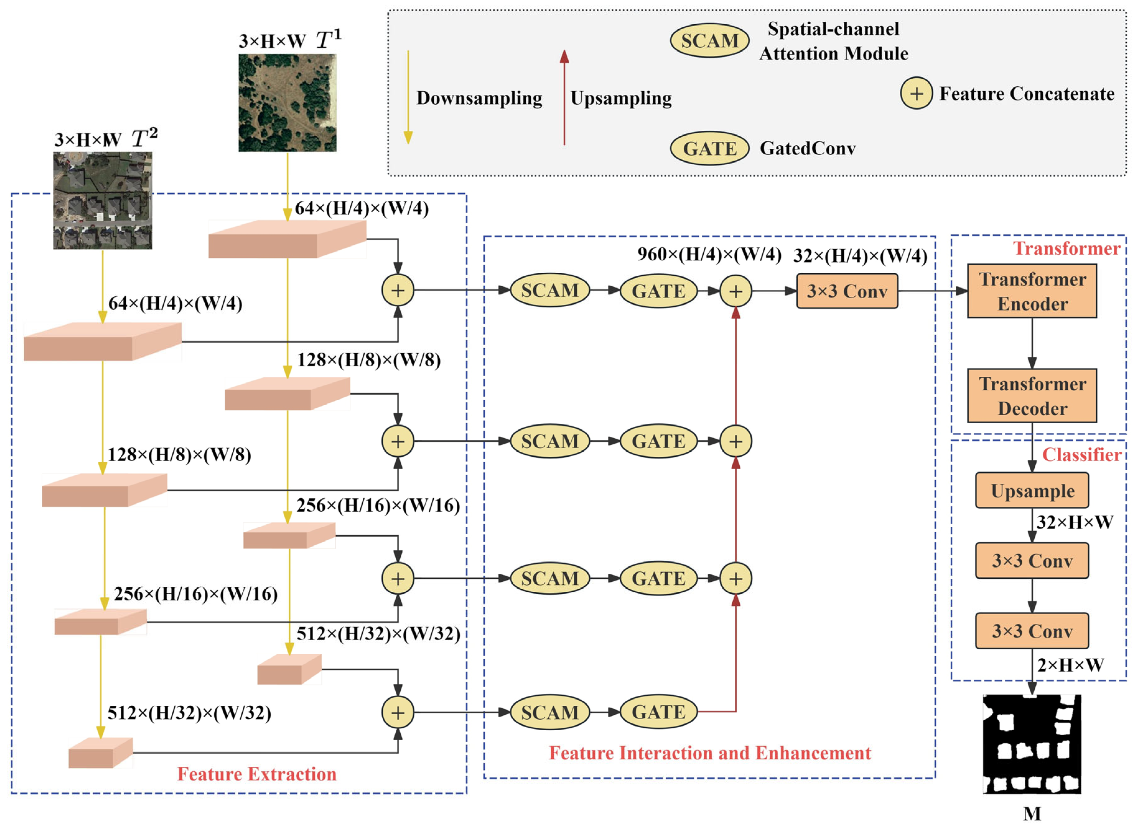
3.1. DFANet Overview
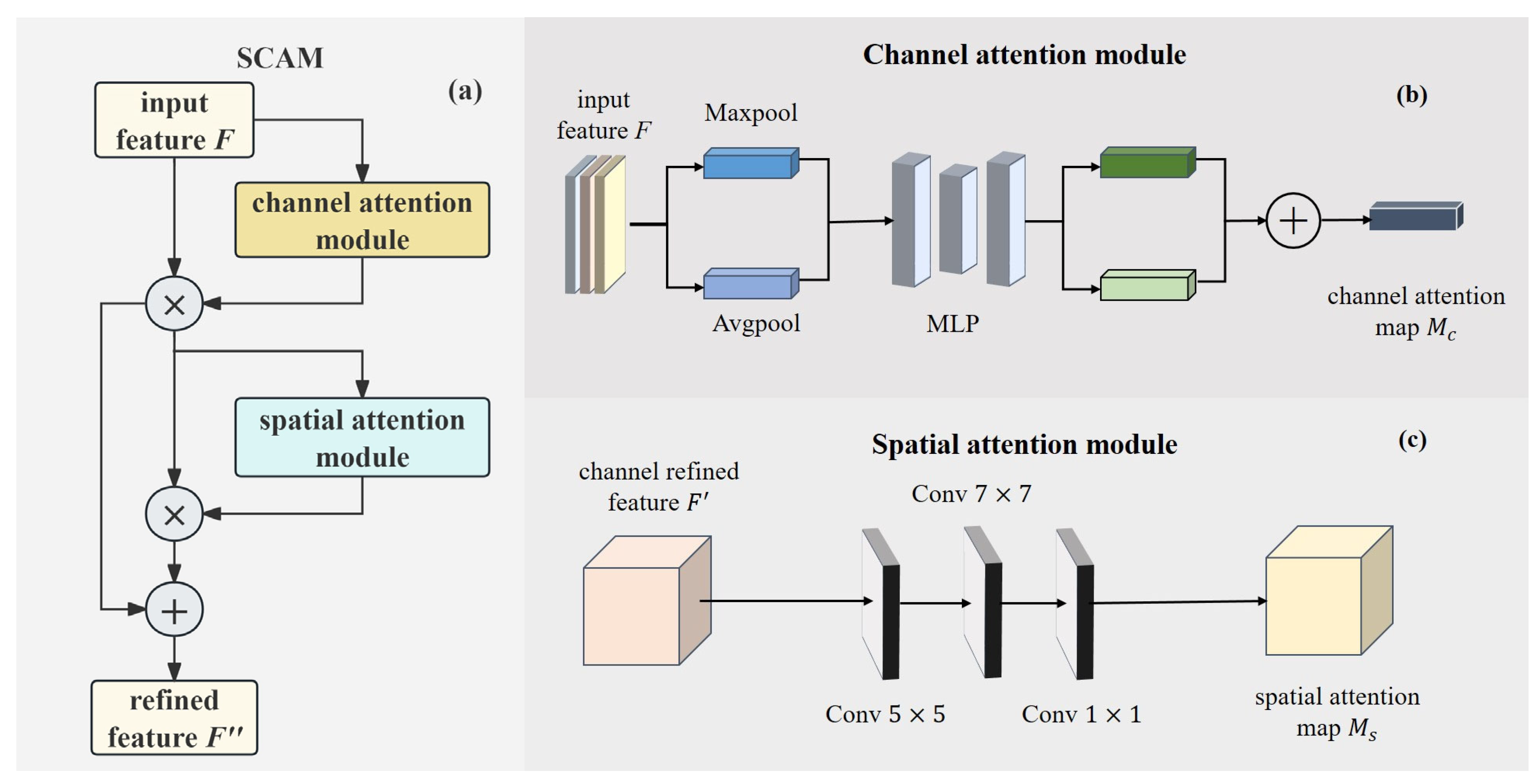
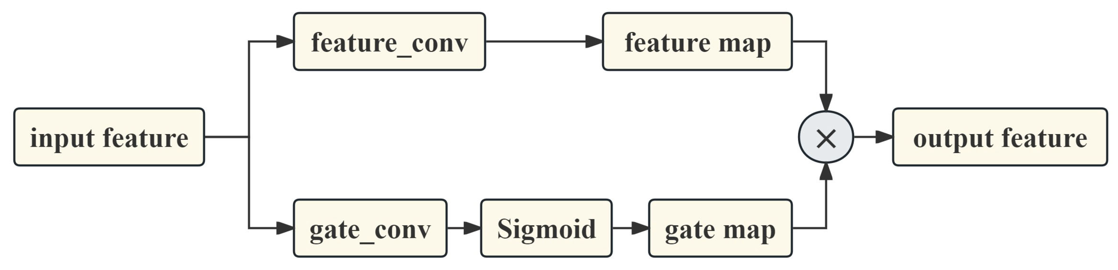
3.2. Deep Feature Attention
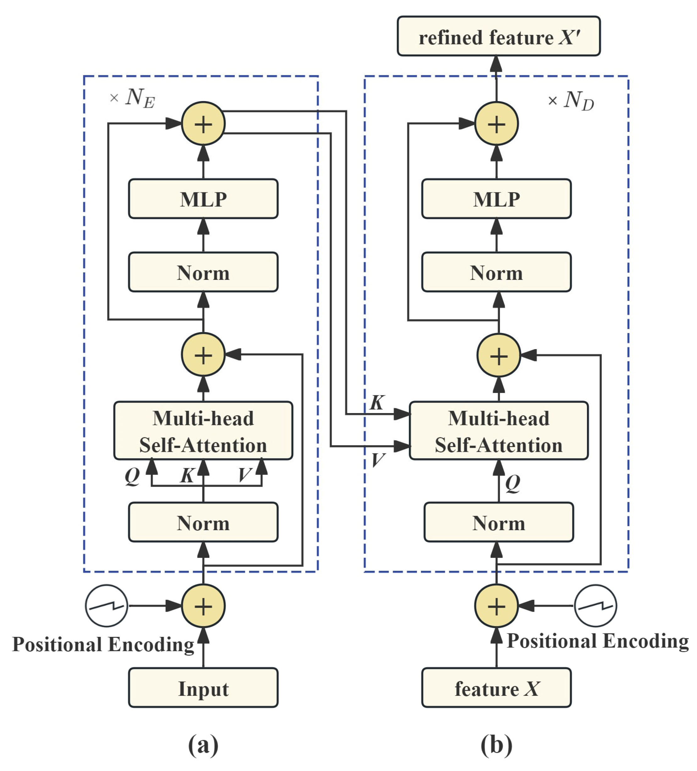
3.3. Transformer
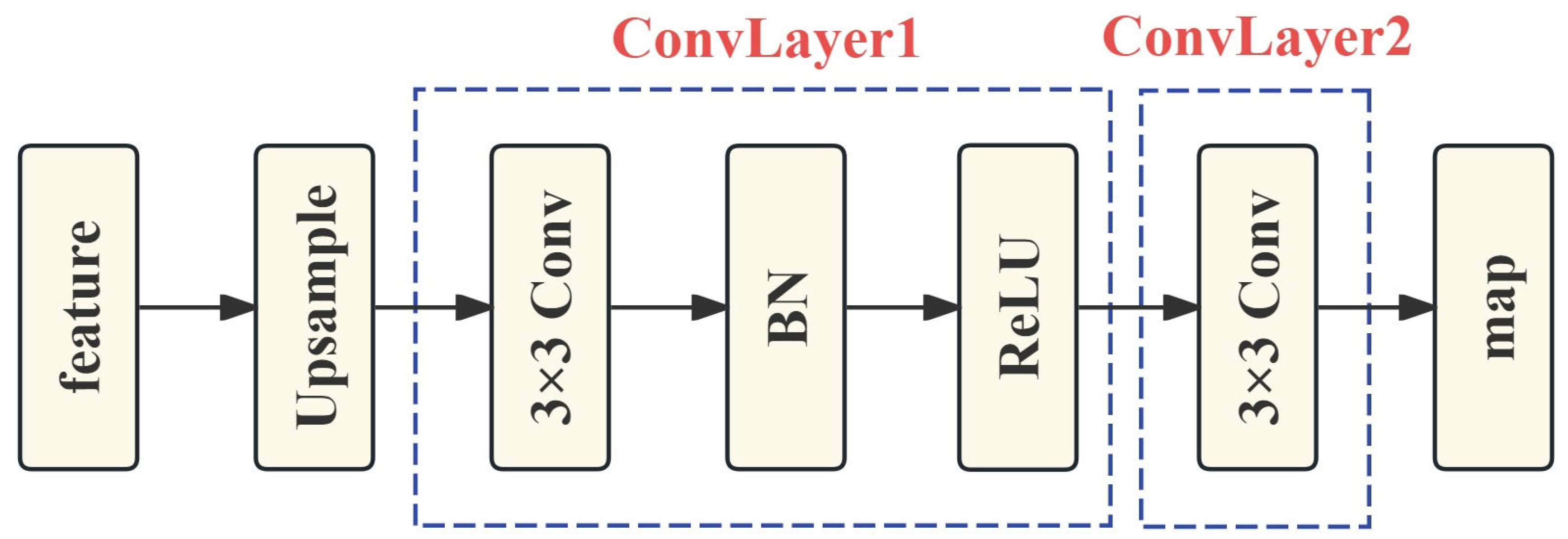
3.4. Classifier
4. Experimental Results and Analysis
4.1. Datasets
- (1)
- LEVIR-CD [43]: A public large-scale building CD dataset. It consists of 637 pairs of high-resolution (0.5-m) image patches, each sized at 1024 × 1024 pixels. These bitemporal images were collected from multiple cities in Texas, USA, spanning a timeframe of 5 to 14 years. We cropped the images into non-overlapping 256 × 256 patches and partitioned them according to the official training, validation, and test splits, resulting in 7120 pairs for training, 1024 pairs for validation, and 2048 pairs for testing. The dataset can be obtained from https://justchenhao.github.io/LEVIR/ (accessed on 10 October 2022).
- (2)
- WHU-CD [44]: A public building CD dataset, namely the high-resolution aerial imagery building CD dataset released by the GPCV Group at Wuhan University in 2019. It contains a pair of high-resolution aerial images with a resolution of 0.075 m and a size of 32,507 × 15,354 pixels. The images were cropped into non-overlapping patches of 256 × 256 pixels, which were randomly partitioned into three subsets: 6096 pairs for training, 762 pairs for validation, and 762 pairs for testing. The dataset can be obtained from https://gpcv.whu.edu.cn/data/building_dataset.html (accessed on 1 October 2023).
4.2. Implementation Details and Evaluation Metrics
4.3. Comparison Methods
- (1)
- FC-EF [24]: An early fusion approach where bitemporal images are channel-wise concatenated to form a multi-channel feature volume, which is then processed through a UNet-based encoder-decoder architecture to generate a pixel-wise change detection map.
- (2)
- FC-Siam-Conc [24]: A late fusion variant of FC-EF that employs dual parallel backbone networks to extract hierarchical features from bitemporal images;
- (3)
- FC-Siam-Diff [24]: A late fusion variant akin to FC-Siam-Conc, which extracts hierarchical features via twin backbones and fuses diachronic information by concatenating absolute differences of corresponding-level features before feeding into a UNet decoder for change map generation;
- (4)
- SNUNet-CD [27]: A hierarchical feature fusion architecture that integrates a Siamese network with UNet++ for CD. It employs dense skip connections between encoders and decoders to propagate high-resolution bitemporal features, enabling multi-scale context aggregation;
- (5)
- BIT [36]: A Transformer-based CD approach that employs a Transformer encoder-decoder framework to extract contextual dependencies from features. It integrates an augmented semantically labeled CNN for multi-scale feature extraction, followed by element-wise feature differencing to generate change maps;
- (6)
- ICIFNet [35]: A CD framework integrating CNN and Transformer, which enhances complex scene performance via same-scale cross-modal interaction and hierarchical cross-scale fusion;
- (7)
- EATDer [45]: An Edge-Assisted Adaptive Transformer designed for remote sensing change detection. EATDer integrates edge information to guide feature extraction and employs a multi-scale adaptive attention mechanism to enhance detection accuracy.
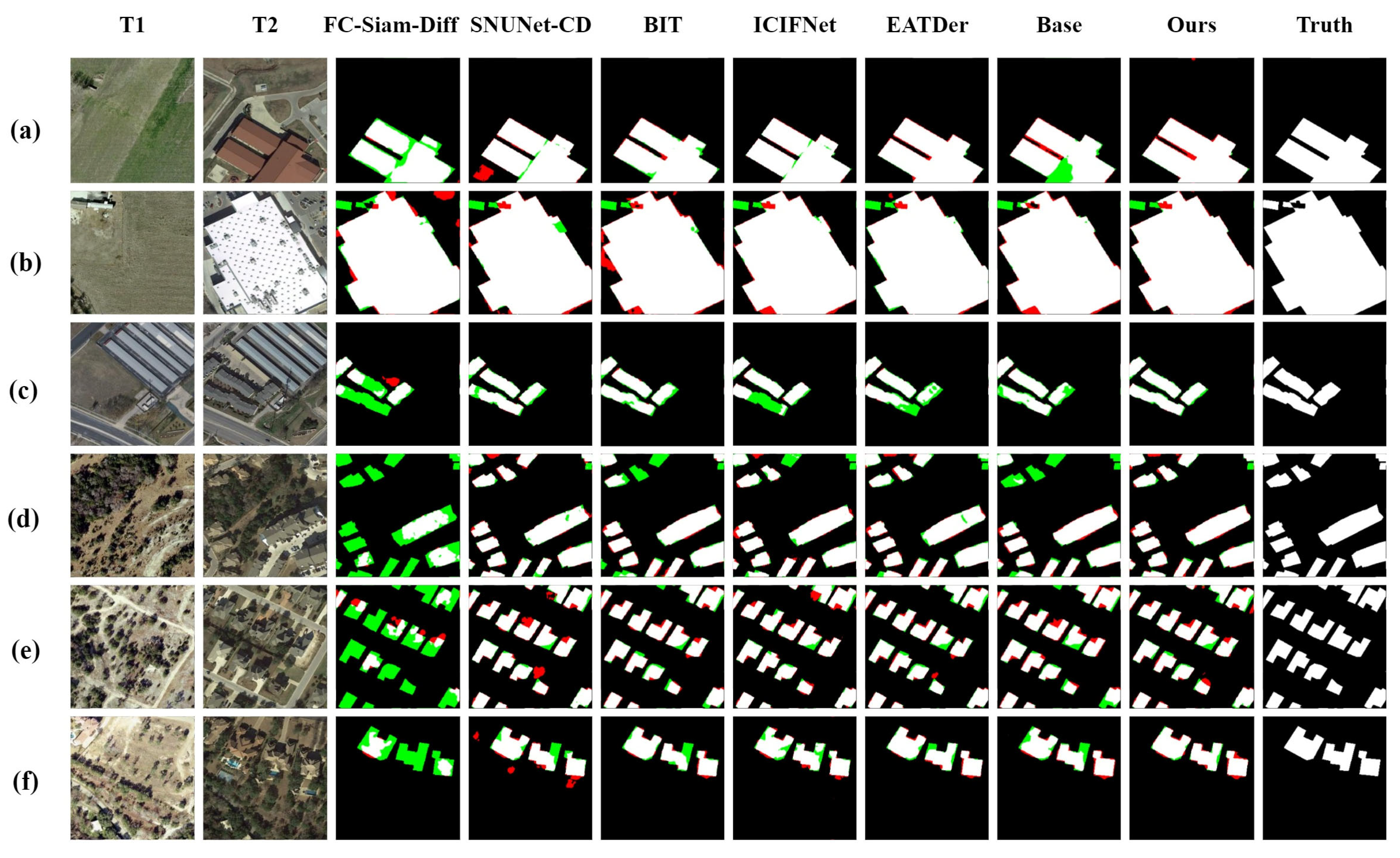
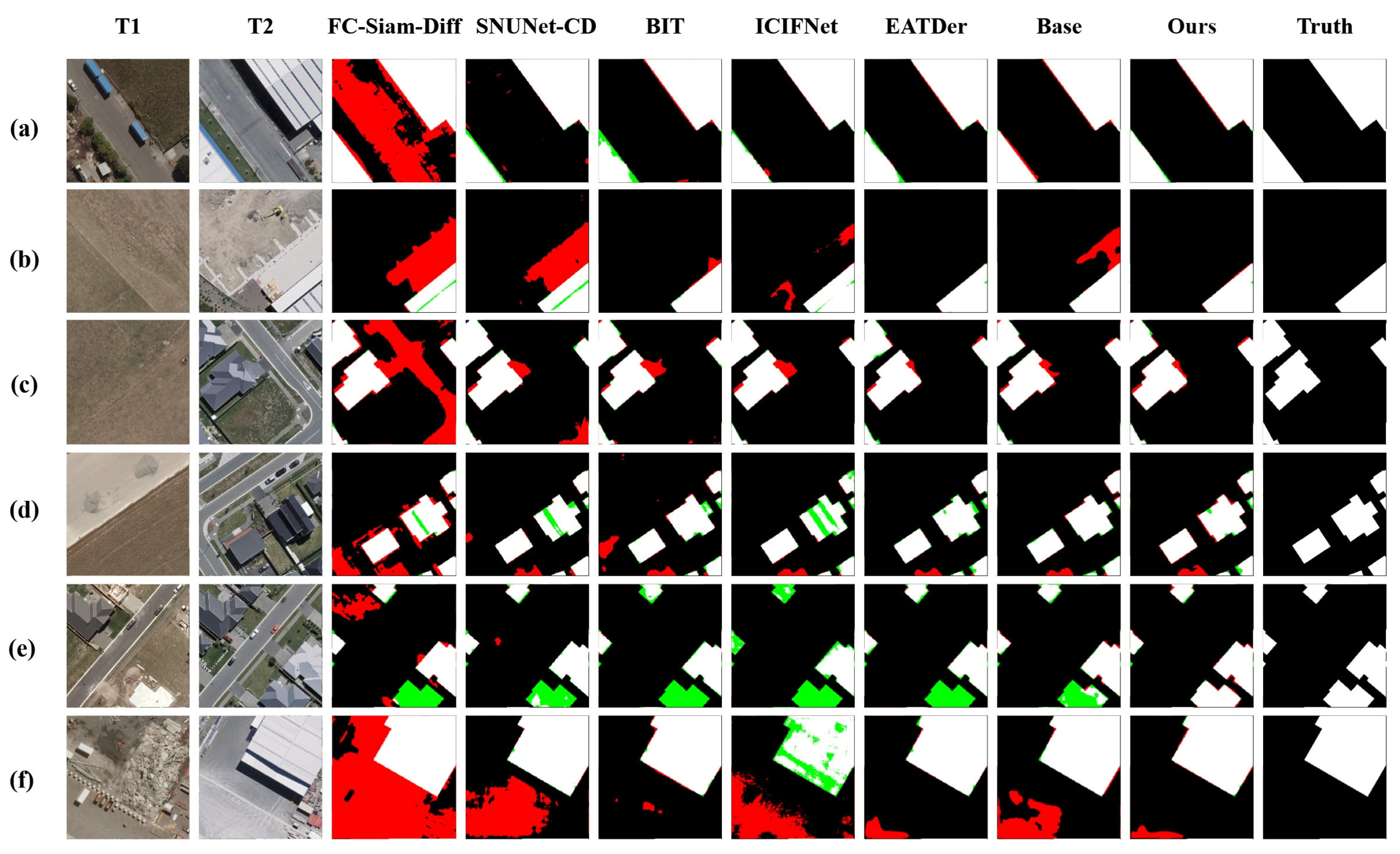
4.4. Results Evaluation
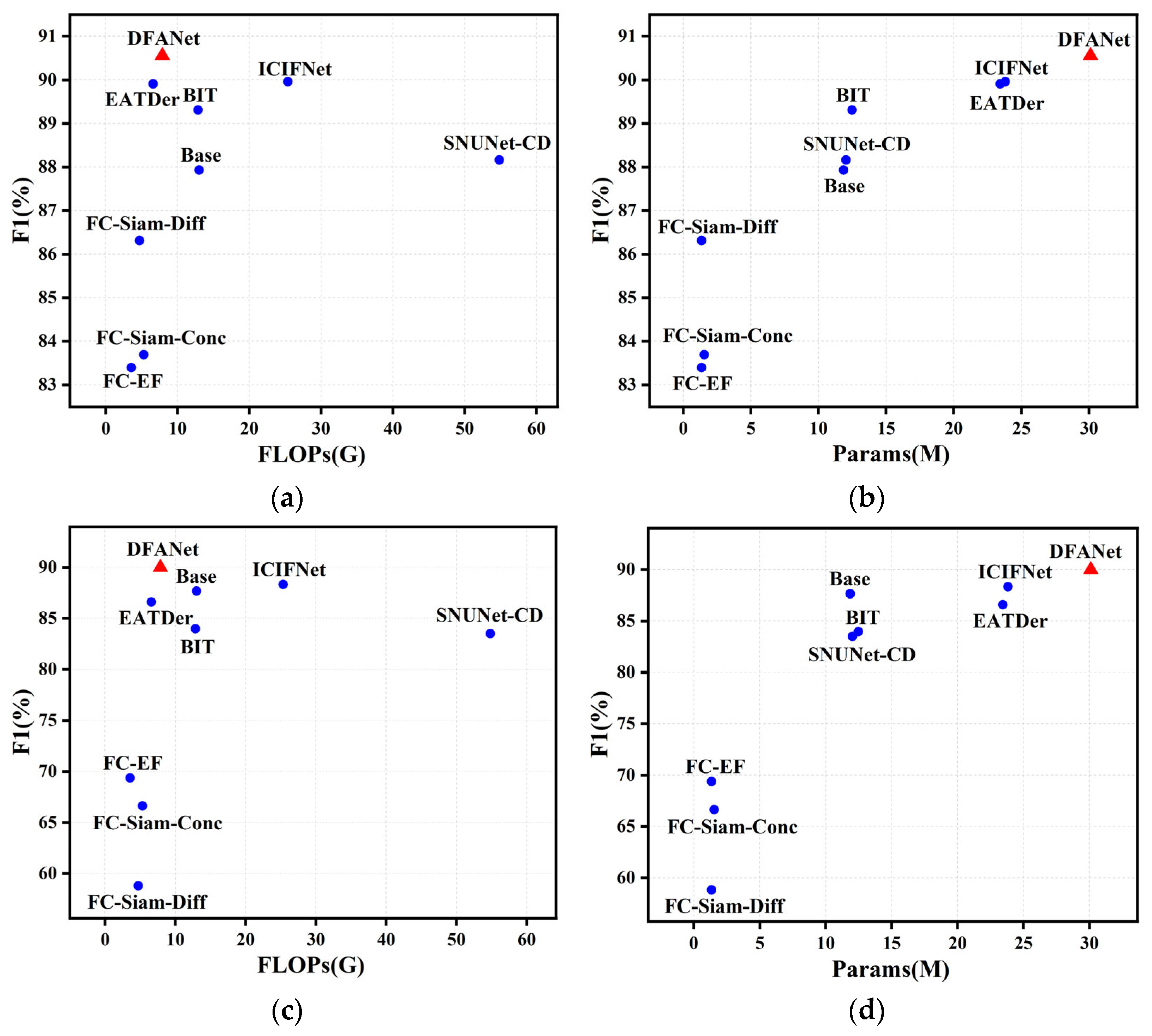
4.5. Complexity Analysis and Significance Test
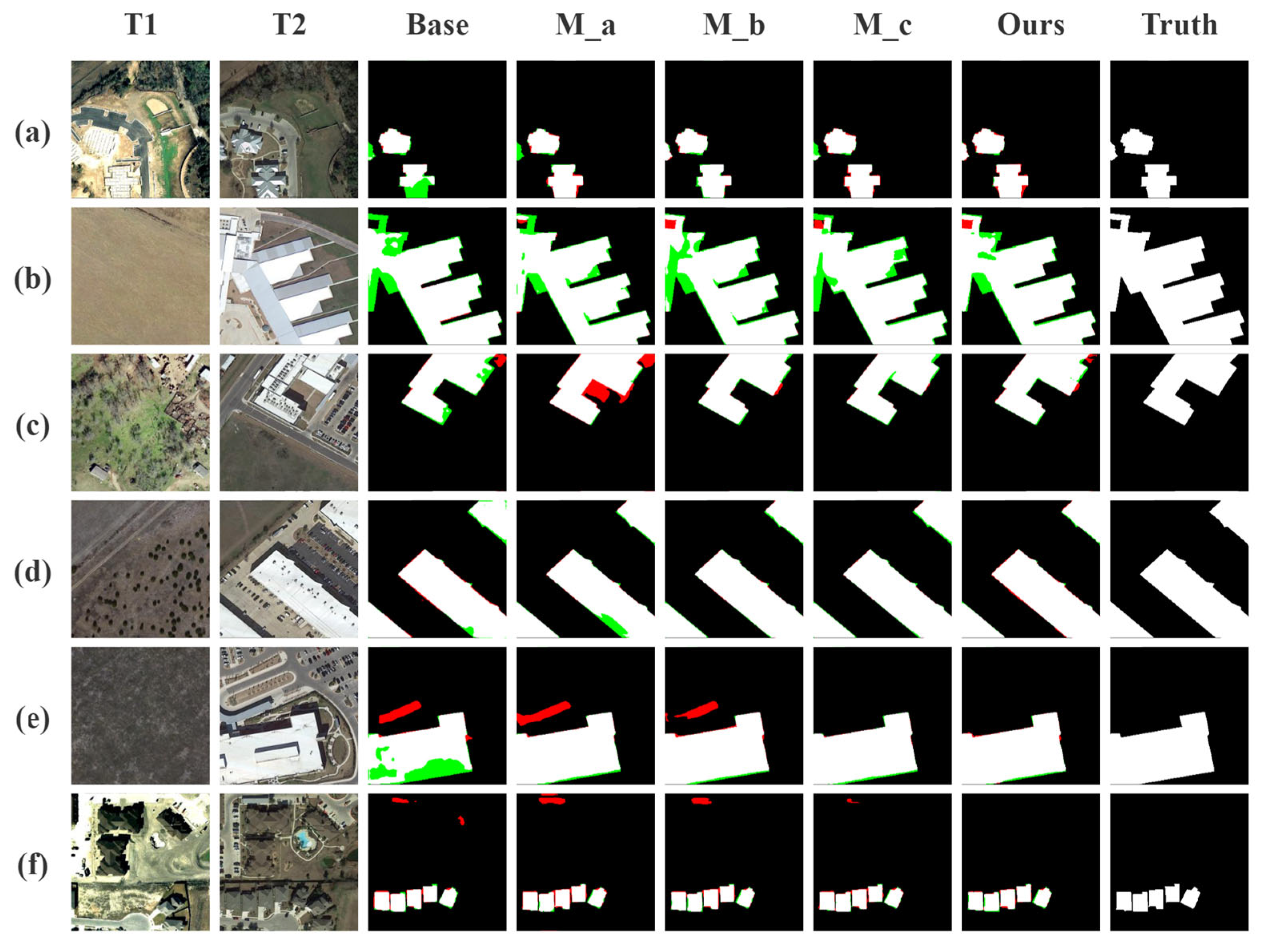
4.6. Ablation Study
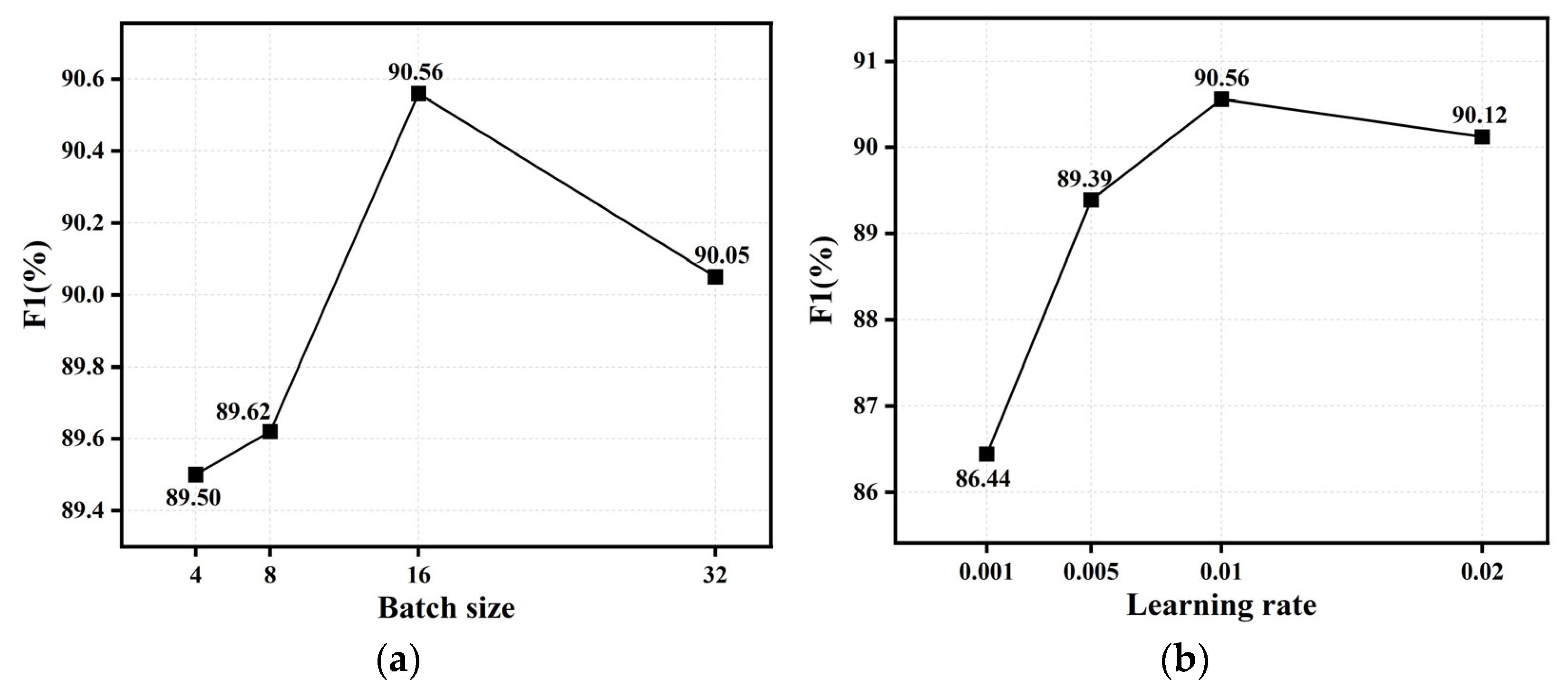
4.7. Parameter Analysis
5. Discussion
6. Conclusions
Author Contributions
Funding
Data Availability Statement
Conflicts of Interest
Abbreviations
| DFANet | Deep Feature Attention Network |
| FC-EF | Fully Convolutional-Early Fusion |
| FC-Siam-Diff | Fully Convolutional-Siamese-Difference |
| FC-Siam-Conc | Fully Convolutional-Siamese-Concatenation |
| SNUNet-CD | Siamese NestedUNet for Change Detection |
| BIT | Bitemporal Image Transformer |
| ICIFNet | Intra-scale Cross-interaction and Inter-scale Feature Fusion Network |
| CBAM | Convolutional Block Attention Module |
| SCAM | Spatial-Channel Attention Module |
| CNN | Convolutional Neural Network |
| CD | Change Detection |
| RS | Remote Sensing |
| DL | Deep Learning |
| ML | Machine Learning |
| GELU | Gaussian Error Linear Unit |
References
- De Bem, P.P.; de Carvalho Junior, O.A.; Fontes Guimarães, R.; Trancoso Gomes, R.A. Change detection of deforestation in the Brazilian Amazon using landsat data and convolutional neural networks. Remote Sens. 2020, 12, 901. [Google Scholar] [CrossRef]
- Kennedy, R.E.; Townsend, P.A.; Gross, J.E.; Cohen, W.B.; Bolstad, P.; Wang, Y.; Adams, P. Remote sensing change detection tools for natural resource managers: Understanding concepts and tradeoffs in the design of landscape monitoring projects. Remote Sens. Environ. 2009, 113, 1382–1396. [Google Scholar] [CrossRef]
- Hawash, E.; El-Hassanin, A.; Amer, W.; El-Nahry, A.; Effat, H. Change detection and urban expansion of Port Sudan, Red Sea, using remote sensing and GIS. Environ. Monit. Assess. 2021, 193, 723. [Google Scholar] [CrossRef] [PubMed]
- Qing, Y.; Ming, D.; Wen, Q.; Weng, Q.; Xu, L.; Chen, Y.; Zhang, Y.; Zeng, B. Operational earthquake-induced building damage assessment using CNN-based direct remote sensing change detection on superpixel level. Int. J. Appl. Earth Observ. Geoinf. 2022, 112, 102899. [Google Scholar] [CrossRef]
- Zhang, Z.; Jiang, H.; Pang, S.; Hu, X. Research Status and Prospects of Change Detection for Multi-Temporal Remote Sensing Images. J. Geomatics. 2022, 51, 1091–1107. [Google Scholar]
- Coppin, P.; Jonckheere, I.; Nackaerts, K.; Muys, B.; Lambin, E. Review ArticleDigital change detection methods in ecosystem monitoring: A review. Int. J. Remote Sens. 2004, 25, 1565–1596. [Google Scholar] [CrossRef]
- Howarth, P.J.; Wickware, G.M. Procedures for change detection using Landsat digital data. Int. J. Remote Sens. 1981, 2, 277–291. [Google Scholar] [CrossRef]
- Dai, X.; Khorram, S. Quantification of the impact of misregistration on the accuracy of remotely sensed change detection. In Proceedings of the IGARSS’97. 1997 IEEE International Geoscience and Remote Sensing Symposium Proceedings. Remote Sensing-A Scientific Vision for Sustainable Development, Singapore, 3–8 August 1997; pp. 1763–1765. [Google Scholar]
- Celik, T. Unsupervised change detection in satellite images using principal component analysis and $ k $-means clustering. IEEE Geosci. Remote Sens. Lett. 2009, 6, 772–776. [Google Scholar] [CrossRef]
- Han, T.; Wulder, M.A.; White, J.C.; Coops, N.C.; Alvarez, M.; Butson, C. An efficient protocol to process Landsat images for change detection with tasselled cap transformation. IEEE Geosci. Remote Sens. Lett. 2007, 4, 147–151. [Google Scholar] [CrossRef]
- Habib, T.; Inglada, J.; Mercier, G.; Chanussot, J. Support vector reduction in SVM algorithm for abrupt change detection in remote sensing. IEEE Geosci. Remote Sens. Lett. 2009, 6, 606–610. [Google Scholar] [CrossRef]
- Zong, K.; Sowmya, A.; Trinder, J. Building change detection from remotely sensed images based on spatial domain analysis and Markov random field. J. Appl. Remote Sens. 2019, 13, 024514. [Google Scholar] [CrossRef]
- Im, J.; Jensen, J.R. A change detection model based on neighborhood correlation image analysis and decision tree classification. Remote Sens. Environ. 2005, 99, 326–340. [Google Scholar] [CrossRef]
- Seo, D.K.; Kim, Y.H.; Eo, Y.D.; Park, W.Y.; Park, H.C. Generation of radiometric, phenological normalized image based on random forest regression for change detection. Remote Sens. 2017, 9, 1163. [Google Scholar] [CrossRef]
- Feng, W.; Sui, H.; Tu, J.; Huang, W.; Sun, K. A novel change detection approach based on visual saliency and random forest from multi-temporal high-resolution remote-sensing images. Int. J. Remote Sens. 2018, 39, 7998–8021. [Google Scholar] [CrossRef]
- Ball, J.E.; Anderson, D.T.; Chan, C.S. Comprehensive survey of deep learning in remote sensing: Theories, tools, and challenges for the community. J. Appl. Remote Sens. 2017, 11, 042609. [Google Scholar] [CrossRef]
- Simonyan, K.; Zisserman, A. Very deep convolutional networks for large-scale image recognition. arXiv 2014, arXiv:1409.1556. [Google Scholar]
- Ronneberger, O.; Fischer, P.; Brox, T. U-net: Convolutional networks for biomedical image segmentation. In Proceedings of the Medical Image Computing and Computer-Assisted Intervention–MICCAI 2015: 18th International Conference, Munich, Germany, 5–9 October 2015; part III 18. pp. 234–241. [Google Scholar]
- He, K.; Zhang, X.; Ren, S.; Sun, J. Deep residual learning for image recognition. In Proceedings of the IEEE Conference on Computer Vision and Pattern Recognition, Las Vegas, NV, USA, 27–30 June 2016; pp. 770–778. [Google Scholar]
- Peng, D.; Bruzzone, L.; Zhang, Y.; Guan, H.; Ding, H.; Huang, X. SemiCDNet: A semisupervised convolutional neural network for change detection in high resolution remote-sensing images. IEEE Trans. Geosci. Remote Sens. 2020, 59, 5891–5906. [Google Scholar] [CrossRef]
- Liu, Y.; Pang, C.; Zhan, Z.; Zhang, X.; Yang, X. Building change detection for remote sensing images using a dual-task constrained deep siamese convolutional network model. IEEE Geosci. Remote Sens. Lett. 2020, 18, 811–815. [Google Scholar] [CrossRef]
- Zhang, C.; Yue, P.; Tapete, D.; Jiang, L.; Shangguan, B.; Huang, L.; Liu, G. A deeply supervised image fusion network for change detection in high resolution bi-temporal remote sensing images. ISPRS J. Photogramm. Remote Sens. 2020, 166, 183–200. [Google Scholar] [CrossRef]
- Chen, J.; Yuan, Z.; Peng, J.; Chen, L.; Huang, H.; Zhu, J.; Liu, Y.; Li, H. DASNet: Dual attentive fully convolutional Siamese networks for change detection in high-resolution satellite images. IEEE J. Sel. Top. Appl. Earth Observ. Remote Sens. 2020, 14, 1194–1206. [Google Scholar] [CrossRef]
- Daudt, R.C.; Le Saux, B.; Boulch, A. Fully convolutional siamese networks for change detection. In Proceedings of the 2018 25th IEEE International Conference on Image Processing (ICIP), Athens, Greece, 7–10 October 2018; pp. 4063–4067. [Google Scholar]
- Peng, D.; Zhang, Y.; Guan, H. End-to-end change detection for high resolution satellite images using improved UNet++. Remote Sens. 2019, 11, 1382. [Google Scholar] [CrossRef]
- Liu, R.; Jiang, D.; Zhang, L.; Zhang, Z. Deep depthwise separable convolutional network for change detection in optical aerial images. IEEE J. Sel. Top. Appl. Earth Observ. Remote Sens. 2020, 13, 1109–1118. [Google Scholar] [CrossRef]
- Fang, S.; Li, K.; Shao, J.; Li, Z. SNUNet-CD: A densely connected Siamese network for change detection of VHR images. IEEE Geosci. Remote Sens. Lett. 2021, 19, 1–5. [Google Scholar] [CrossRef]
- Shi, Q.; Liu, M.; Li, S.; Liu, X.; Wang, F.; Zhang, L. A deeply supervised attention metric-based network and an open aerial image dataset for remote sensing change detection. IEEE Trans. Geosci. Remote Sens. 2021, 60, 1–16. [Google Scholar] [CrossRef]
- Woo, S.; Park, J.; Lee, J.-Y.; Kweon, I.S. Cbam: Convolutional block attention module. In Proceedings of the European conference on computer vision (ECCV), Munich, Germany, 8–14 September 2018; pp. 3–19. [Google Scholar]
- Guo, E.; Fu, X.; Zhu, J.; Deng, M.; Liu, Y.; Zhu, Q.; Li, H. Learning to measure change: Fully convolutional siamese metric networks for scene change detection. arXiv 2018, arXiv:1810.09111. [Google Scholar] [CrossRef]
- Li, Z.; Yan, C.; Sun, Y.; Xin, Q. A densely attentive refinement network for change detection based on very-high-resolution bitemporal remote sensing images. IEEE Trans. Geosci. Remote Sens. 2022, 60, 1–18. [Google Scholar] [CrossRef]
- Chen, P.; Zhang, B.; Hong, D.; Chen, Z.; Yang, X.; Li, B. FCCDN: Feature constraint network for VHR image change detection. ISPRS J. Photogramm. Remote Sens. 2022, 187, 101–119. [Google Scholar] [CrossRef]
- Vaswani, A.; Shazeer, N.; Parmar, N.; Uszkoreit, J.; Jones, L.; Gomez, A.N.; Kaiser, Ł.; Polosukhin, I. Attention is all you need. arXiv 2017, arXiv:1706.03762. [Google Scholar]
- Zhang, C.; Wang, L.; Cheng, S.; Li, Y. SwinSUNet: Pure transformer network for remote sensing image change detection. IEEE Trans. Geosci. Remote Sens. 2022, 60, 1–13. [Google Scholar] [CrossRef]
- Feng, Y.; Xu, H.; Jiang, J.; Liu, H.; Zheng, J. ICIF-Net: Intra-scale cross-interaction and inter-scale feature fusion network for bitemporal remote sensing images change detection. IEEE Trans. Geosci. Remote Sens. 2022, 60, 1–13. [Google Scholar] [CrossRef]
- Chen, H.; Qi, Z.; Shi, Z. Remote sensing image change detection with transformers. IEEE Trans. Geosci. Remote Sens. 2021, 60, 1–14. [Google Scholar] [CrossRef]
- Jian, P.; Ou, Y.; Chen, K. Uncertainty-aware graph self-supervised learning for hyperspectral image change detection. IEEE Trans. Geosci. Remote Sens. 2024, 62, 1–19. [Google Scholar] [CrossRef]
- Pang, S.; Lan, J.; Zuo, Z.; Chen, J. SFGT-CD: Semantic Feature-Guided Building Change Detection from Bitemporal Remote-Sensing Images with Transformers. IEEE Geosci. Remote Sens. Lett. 2023, 21, 1–5. [Google Scholar] [CrossRef]
- Lu, W.; Wei, L.; Nguyen, M. Bitemporal Attention Transformer for Building Change Detection and Building Damage Assessment. IEEE J. Sel. Top. Appl. Earth Obs. Remote Sens. 2024, 17, 4917–4935. [Google Scholar] [CrossRef]
- Guo, M.H.; Lu, C.Z.; Liu, Z.N.; Cheng, M.M.; Hu, S.M. Visual Attention Network. arXiv 2022, arXiv:2022.09741. [Google Scholar] [CrossRef]
- Patro, B.N.; Namboodiri, V.P.; Agneeswaran, V.S. Spectformer: Frequency and attention is what you need in a vision transformer. In Proceedings of the 2025 IEEE/CVF Winter Conference on Applications of Computer Vision (WACV), Tucson, AZ, USA, 26 February–6 March 2025; pp. 9543–9554. [Google Scholar]
- Hendrycks, D.; Gimpel, K. Gaussian error linear units (gelus). arXiv 2016, arXiv:1606.08415. [Google Scholar]
- Chen, H.; Shi, Z. A spatial-temporal attention-based method and a new dataset for remote sensing image change detection. Remote Sens. 2020, 12, 1662. [Google Scholar] [CrossRef]
- Ji, S.; Wei, S.; Lu, M. Fully convolutional networks for multisource building extraction from an open aerial and satellite imagery data set. IEEE Trans. Geosci. Remote Sens. 2018, 57, 574–586. [Google Scholar] [CrossRef]
- Ma, J.; Duan, J.; Tang, X.; Zhang, X.; Jiao, L. EATDer: Edge-Assisted Adaptive Transformer Detector for Remote Sensing Change Detection. IEEE Trans. Geosci. Remote Sens. 2024, 62, 5602015. [Google Scholar] [CrossRef]
- Manandhar, R.; Odeh, I.O.; Ancev, T. Improving the accuracy of land use and land cover classification of Landsat data using post-classification enhancement. Remote Sens. 2009, 1, 330–344. [Google Scholar] [CrossRef]


| Methods | Pre | Rec | F1 | IoU | OA |
|---|---|---|---|---|---|
| FC-EF [24] | 86.91 | 80.17 | 83.40 | 71.53 | 98.39 |
| FC-Siam-Diff [24] | 89.53 | 83.31 | 86.31 | 75.92 | 98.67 |
| FC-Siam-Conc [24] | 91.99 | 76.77 | 83.69 | 71.96 | 98.49 |
| SNUNet-CD [27] | 89.18 | 87.17 | 88.16 | 78.83 | 98.82 |
| BIT [36] | 89.24 | 89.37 | 89.31 | 80.68 | 98.92 |
| ICIFNet [35] | 91.32 | 88.64 | 89.96 | 81.75 | 98.99 |
| EATDer [45] | 88.13 | 91.77 | 89.91 | 81.68 | 98.95 |
| Base | 90.64 | 85.39 | 87.93 | 78.46 | 98.81 |
| DFANet (Ours) | 91.87 | 89.29 | 90.56 | 82.75 | 99.05 |
| Methods | Pre | Rec | F1 | IoU | OA |
|---|---|---|---|---|---|
| FC-EF [24] | 71.63 | 67.25 | 69.37 | 53.11 | 97.61 |
| FC-Siam-Diff [24] | 47.33 | 77.66 | 58.81 | 41.66 | 95.63 |
| FC-Siam-Conc [24] | 60.88 | 73.58 | 66.63 | 49.95 | 97.04 |
| SNUNet-CD [27] | 85.60 | 81.49 | 83.50 | 71.67 | 98.71 |
| BIT [36] | 86.64 | 81.48 | 83.98 | 72.39 | 98.75 |
| ICIFNet [35] | 92.98 | 85.56 | 88.32 | 79.24 | 98.96 |
| EATDer [45] | 86.38 | 86.82 | 86.60 | 76.36 | 98.88 |
| Base | 86.26 | 89.09 | 87.66 | 78.02 | 99.04 |
| DFANet (Ours) | 92.32 | 87.75 | 89.98 | 81.78 | 99.22 |
| Methods | FLOPs (G) | Params (M) | F1 (%) | |
|---|---|---|---|---|
| LEVIR-CD | WHU-CD | |||
| FC-EF [24] | 3.57 | 1.35 | 83.40 | 69.37 |
| FC-Siam-Diff [24] | 4.72 | 1.35 | 86.31 | 58.81 |
| FC-Siam-Conc [24] | 5.32 | 1.55 | 83.69 | 66.63 |
| SNUNet-CD [27] | 54.83 | 12.03 | 88.16 | 83.50 |
| BIT [36] | 12.85 | 13.48 | 89.31 | 83.98 |
| ICIFNet [35] | 25.36 | 23.82 | 89.96 | 88.32 |
| EATDer [45] | 6.60 | 23.43 | 89.91 | 86.60 |
| Base | 13.01 | 11.85 | 87.93 | 87.66 |
| DFANet (Ours) | 7.88 | 30.11 | 90.56 | 89.98 |
| Methods | LEVIR-CD | WHU-CD | ||||||
|---|---|---|---|---|---|---|---|---|
| A × 106 | B × 106 | X2 × 106 | p | A × 106 | B × 106 | X2 × 106 | p | |
| FC-Siam-Diff [24] | 2.1847 | 0.5207 | 1.0234 | <0.001 | 6.7196 | 0.1347 | 6.3260 | <0.001 |
| SNUNet-CD [27] | 0.4223 | 0.2651 | 0.0359 | <0.001 | 0.2546 | 0.1539 | 0.0248 | <0.001 |
| BIT [36] | 0.4765 | 0.3368 | 0.0240 | <0.001 | 0.3628 | 0.1319 | 0.1078 | <0.001 |
| ICIFNet [35] | 0.5401 | 0.4564 | 0.0070 | <0.001 | 0.4445 | 0.1399 | 0.1588 | <0.001 |
| EATDer [45] | 0.3276 | 0.2624 | 0.0072 | <0.001 | 0.1487 | 0.0786 | 0.0216 | <0.001 |
| Base | 0.6786 | 0.4236 | 0.0590 | <0.001 | 0.2167 | 0.1437 | 0.0148 | <0.001 |
| Methods | SCAM | GatedConv | Transformer | Pre | Rec | F1 | IoU | OA | FLOPs (G) | Params (M) |
|---|---|---|---|---|---|---|---|---|---|---|
| Base | 90.64 | 85.39 | 87.93 | 78.46 | 98.81 | 13.01 | 11.85 | |||
| M_a | √ | 90.39 | 89.85 | 90.12 | 82.01 | 98.99 | 5.99 | 26.21 | ||
| M_b | √ | √ | 91.24 | 89.07 | 90.14 | 82.06 | 99.01 | 7.27 | 26.88 | |
| M_c | √ | √ | 91.20 | 89.43 | 90.30 | 82.33 | 99.02 | 6.60 | 28.44 | |
| DFANet (Ours) | √ | √ | √ | 91.87 | 89.29 | 90.56 | 82.75 | 99.05 | 7.88 | 30.11 |
| NE | ND | F1 (%) | |
|---|---|---|---|
| LEVIR-CD | WHU-CD | ||
| 1 | 1 | 90.56 | 89.98 |
| 1 | 4 | 90.63 | 90.03 |
| 1 | 8 | 90.65 | 90.08 |
| 2 | 4 | 90.49 | 89.90 |
Disclaimer/Publisher’s Note: The statements, opinions and data contained in all publications are solely those of the individual author(s) and contributor(s) and not of MDPI and/or the editor(s). MDPI and/or the editor(s) disclaim responsibility for any injury to people or property resulting from any ideas, methods, instructions or products referred to in the content. |
© 2025 by the authors. Licensee MDPI, Basel, Switzerland. This article is an open access article distributed under the terms and conditions of the Creative Commons Attribution (CC BY) license (https://creativecommons.org/licenses/by/4.0/).
Share and Cite
Lu, P.; Ding, H.; Tian, X. DFANet: A Deep Feature Attention Network for Building Change Detection in Remote Sensing Imagery. Remote Sens. 2025, 17, 2575. https://doi.org/10.3390/rs17152575
Lu P, Ding H, Tian X. DFANet: A Deep Feature Attention Network for Building Change Detection in Remote Sensing Imagery. Remote Sensing. 2025; 17(15):2575. https://doi.org/10.3390/rs17152575
Chicago/Turabian StyleLu, Peigeng, Haiyong Ding, and Xiang Tian. 2025. "DFANet: A Deep Feature Attention Network for Building Change Detection in Remote Sensing Imagery" Remote Sensing 17, no. 15: 2575. https://doi.org/10.3390/rs17152575
APA StyleLu, P., Ding, H., & Tian, X. (2025). DFANet: A Deep Feature Attention Network for Building Change Detection in Remote Sensing Imagery. Remote Sensing, 17(15), 2575. https://doi.org/10.3390/rs17152575