Abstract
Direct localization methods offer significant advantages in modern high-frequency (HF) radar systems for maritime target localization. However, the presence of amplitude–phase errors poses severe challenges to their accuracy and reliability. Traditional active calibration methods for direct localization often face high costs and operational complexities, while self-calibration techniques are limited to addressing only single or, at most, two types of error models. To address these issues, the Multi-Station Azimuth-based Position Error Calibration Algorithm (MAPEC) is proposed in this paper, which is an active calibration algorithm to solve mixed amplitude–phase errors in direct positioning. The proposed algorithm converts the estimated amplitude–phase errors on each angle of stations into the corresponding position on the localization search grid and adjusts the steering vectors based on the converted errors. By integrating MAPEC with direct localization algorithms, the method enables precise and robust localization under complex amplitude–phase error conditions involving multiple error sources. Simulation results demonstrate that this approach significantly improves localization accuracy across various error conditions, validating its applicability to direct localization applications.
1. Introduction
High-frequency (HF) radar has gained significant popularity in maritime target localization due to its extensive coverage and high-resolution capabilities [1,2,3,4,5]. However, achieving high positioning accuracy is often hindered by amplitude–phase errors during the localization process.
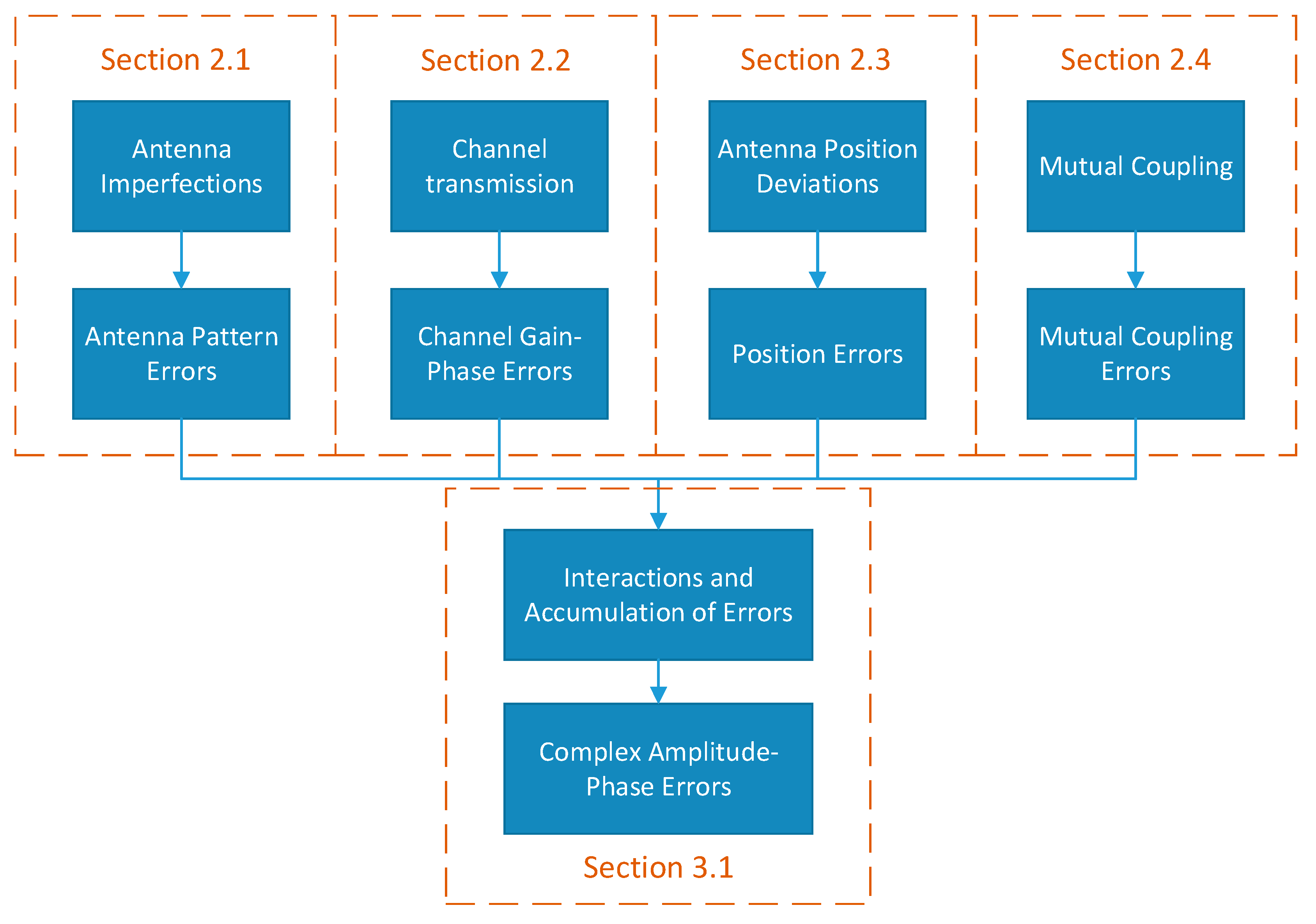
The amplitude–phase errors can be categorized into four main types. Antenna pattern errors refer to deviations between the actual antenna pattern of each element and its ideal pattern, resulting in directional inaccuracies [6,7]. Channel gain–phase errors arise from discrepancies in the amplitude and phase of signals across different channels, leading to inconsistencies in signal reception [7,8,9,10]. Position errors occur due to misalignments between the actual spatial positions of elements and their ideal positions, causing errors in localization accuracy [10,11]. Mutual coupling errors describe the signal interference and phase distortion caused by interactions between adjacent elements, which can result in signal leakage or phase shifts [8,12].
Among these four types of amplitude–phase errors, all except channel gain–phase errors are direction-dependent, meaning that the magnitude of the errors varies with the incoming signal’s direction. These error sources are critical in HF radar and localization systems, where effective calibration and compensation are crucial for enhancing accuracy and overall system performance. To address the positioning challenges in HF radar systems, researchers have increasingly focused on correcting amplitude–phase errors. Array calibration techniques can be broadly categorized into self-calibration methods, which rely on internal signal processing without the need for external reference signals, and active calibration methods, which utilize known external signals to adjust and compensate for errors.
In the realm of self-calibration algorithms, the explicit calibration method for millimeter-wave phased arrays [13] represents a significant advancement. This algorithm constructs error lookup tables and performs multi-point calibration by measuring the amplitude and phase response across the phase control range of each array element. It effectively addresses scenarios involving mixed amplitude–phase error types. However, this method is specifically designed for phased arrays with integrated phase control modules. In contrast, conventional passive radar arrays, which lack phase control modules, cannot implement this approach. Existing self-calibration algorithms [14,15] for passive radar arrays primarily focus on addressing angle-independent amplitude–phase error types, such as channel gain–phase errors, or angle-dependent errors that exhibit predictable and modellable patterns, such as array position errors and mutual coupling errors. However, these methods are insufficient for handling angle-dependent amplitude–phase errors that vary randomly with direction, such as antenna pattern errors, which remain a significant challenge in passive radar systems.
In practical scenarios, the four types of amplitude–phase errors do not occur independently but rather coexist and interact, forming a complex amplitude–phase error environment. This environment is characterized by direction-dependent errors with irregular variations across angles, making them difficult to model and compute. This paper aims to address the problem of low direct localization accuracy in such conditions. As a result, active calibration algorithms are better suited for this context. Current active calibration methods typically rely on precomputing amplitude–phase errors at multiple angles using known azimuthal emitters [16,17]. For example, the experimental validation method for phased array antenna calibration [18] employs near-field data analysis and sequentially switches array elements to gradually correct amplitude and phase inconsistencies between elements. However, this approach is inherently restricted to phased arrays and cannot be extended to conventional passive arrays. Moreover, active calibration methods based on multiple known reference signals, mobile signal sources, or other active strategies are primarily designed to address amplitude–phase errors in angle estimation problems [19,20,21]. It is worth noting that research on calibration algorithms specifically designed for distributed array direct localization remains an unexplored area.
Conventional localization calibration methods generally consist of two steps: Firstly, angle-of-arrival (AOA) or time-difference-of arrival (TDOA) of each incident signal is estimated; Secondly, the emitters are located by solving an equation set related to the measurements of the first step [22,23,24,25,26]. However, these 2-step methods are often suboptimal because they disregard the internal geometric constraints of the received data. Additionally, for multi-emitter scenarios, an extra data association step is required to accurately link measurements to their corresponding sources.
To address the limitations of traditional 2-step processing, recent studies have explored methods for directly localizing emitters. Unlike conventional 2-step localization algorithms, which first estimate DOAs and then calculate position, the direct localization bypasses DOA estimation entirely, allowing emitters to be localized directly [27,28,29,30]. This direct localization algorithm approach enhances localization robustness, particularly in scenarios with low signal-to-noise ratios (SNR) and limited snapshots (SNAP), where it outperforms traditional TDOA-based methods. Direct localization performs a grid search within the region of interest, where the peaks in the generated spatial spectrum indicate the presence and location of emitters.
This paper employs a complex amplitude–phase error model, where the specific coefficients of amplitude–phase errors vary with each emitter’s position. In this complex model, the relationship between error coefficients and emitter positions cannot be analytically derived, necessitating the use of active calibration. To address this, error coefficients are precomputed at all search grid positions using known signal sources, forming an amplitude–phase error matrix, which is then applied to correct the steering vector matrix. While this approach enables accurate direct localization through grid search in the region of interest, performing active calibration at each search position demands a large number of calibration sources and considerable labor, rendering it nearly impractical.
To enable active calibration under direct localization, this paper proposes a novel approach for correcting amplitude–phase errors in the direct localization of stationary emitters with zero velocity. Rather than conducting global calibration at every search grid position, we introduce a localized strategy in which each station undergoes active calibration at specified search angles. This approach significantly reduces the required number of calibration sources, enhancing the feasibility of the calibration process. The main contributions of this paper are:
- A Multi-Station Azimuth-based Position Error Calibration Algorithm (MAPEC) is proposed to address the impact of errors on localization performance in distributed multi-station direct localization. The MAPEC is integrated with the expectation–maximization (EM) 1-step direct localization algorithm to achieve precise direct localization under complex error conditions, with simulations validating the algorithm’s effectiveness.
- This paper proposes a complex error model for distributed array localization, which considers the combined effects of multiple amplitude–phase error types. The model lays the foundation for addressing the challenge of varying amplitude–phase error values at different positions in the search grid during direct localization.
The structure of this paper is as follows: Section 2 introduces four common types of amplitude and phase errors encountered in DOA estimation. In Section 3, we establish a distributed multi-station localization model under complex error conditions and present the detailed steps of the proposed MAPEC algorithm. Section 4 conducts multiple simulation experiments, and the results demonstrate the effectiveness of the proposed method. Finally, Section 5 discusses the research findings and provides prospects for future work.
Notations: Matrices and vectors are denoted by bold symbols. The superscript denotes transpose, and denotes conjugate transpose. The notation represents transforming a vector to a diagonal matrix.
2. Amplitude–Phase Errors Modeling
For an arbitrary geometric structure of an -antenna planar array, there are () emitters emitting ground waves (with wavelength ) in the far field, with their azimuth vectors denoted as . HF ground wave signals propagate along the sea surface, so the elevation angle (the angle between the signal and the xy-plane) is always considered to be 0°. Selecting the first antenna of the array as the origin, and the plane where the array is located as the xy-plane. As per the knowledge from the previous sections, the received tth snapshot vector of the array can be represented as:
where is an dimensional snapshot data vector, is an dimensional array manifold matrix, represents the array steering vector corresponding to . is the incoming angle of the nth Emitter, , and denotes the set of positive integers. is an dimensional array noise vector, and is an dimensional vector representing the complex amplitude of the incoming signal. When there is no amplitude–phase error in the array antennas, the array steering vector can be expressed as:
where , is the speed of light. is the xy-plane position coordinate of the mth antenna. In practical engineering applications, common array errors include array element pattern errors, channel gain–phase errors, mutual coupling, and antenna position errors. In real-world signal reception scenarios, these four types of errors typically coexist. Their combined and interacting effects form the complex amplitude–phase error conditions that are the focus of this study. The complex amplitude–phase diagram is shown in Figure 1.
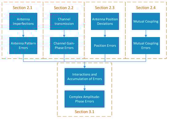
Figure 1.
Illustration of complex amplitude–phase error formation.
The following discussion is mainly concerned with these four kinds of amplitude–phase errors.
2.1. Antenna Pattern Errors
When modeling the array steering vector, it is commonly assumed that the array antennas constituting the array are omnidirectional sensors with identical complex gains. However, in practical engineering applications, the directional patterns of individual antennas cannot be perfectly identical due to sensor fabrication precision errors. The inconsistency in directional patterns can be described by introducing azimuth-dependent amplitude–phase perturbations in the modeling of the steering vector, as follows:
where, , represents the sensor response of antenna at azimuth . Accordingly, the modification of the array manifold matrix in the presence of element pattern errors is as follows:
2.2. Channel Gain–Phase Errors
Channel gain–phase errors refer to complex gain errors that are independent of azimuth, typically arising from the inconsistent gains of amplifiers within the receiving channels. These errors can be described by introducing azimuth-independent amplitude–phase error vectors in the modeling of the steering vector, where represents the amplitude–phase perturbation of mth antenna within the channel, , as follows:
Therefore, when channel gain–phase errors exist, the array manifold matrix can be expressed:
Equation (6) can be considered a special case of Equation (4).
2.3. Position Errors
The array steering vector represents the spatial response of the array to a unit-power spatial source and is closely related to the spatial positions of the array antennas. Different spatial positions correspond to different source propagation delays in modeling the steering vector, leading to different phase responses of the array to spatial sources. Therefore, when there are disturbances in the positions of the antennas, it can be equivalent to introducing azimuth-dependent phase perturbations in the array steering vector:
In Formula (9), and represent the disturbance in the antenna position on the x and y axes, respectively. Thus, the array manifold matrix in the presence of antenna position errors is:
Equation (10) can also be viewed as a special case of Equation (4). The fundamental difference lies in the fact that the error matrix can be analytically expressed by the errors in the positions of the antennas.
2.4. Mutual Coupling Errors
In the modeling of array steering vectors, it is usually assumed that each antenna operates independently of the others. However, the mutual coupling effects between antennas are often inevitable in the practical operation of array antennas, especially at high frequencies. To prevent pattern ambiguity, the spacing between antennas is kept small, making the mutual coupling effects between antennas more pronounced.
Regarding the effects of mutual coupling, they can still be modeled using azimuth-dependent amplitude–phase errors. That is:
where the matrix reflects the mutual coupling effects between antennas. Comparing the amplitude–phase error matrix caused by mutual coupling with that caused by pattern errors, here, the amplitude–phase error matrix can be analytically expressed by the mutual coupling coefficients.
3. Methodology
3.1. Distributed Array Signal Receiving Model with Comprehensive Amplitude–Phase Error
Shown in Figure 2 is the emitter localization system considered in this work, where stationary emitters with zero velocity and separated stations are located in the horizontal plane. In the figure, the red dots represent the positions of the array elements, with groups of closely spaced elements forming a substation. The blue dots represent the emitters. The signals emitted by the emitters propagate along the black lines in the direction indicated by the black arrows and are received by each substation. The angle between the black line and the positive x-axis represents the azimuth angle of the incoming signal.
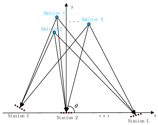
Figure 2.
Emitter localization system.
Each station is equipped with a -antenna () array. Let denote the positions of the emitters, where . The data received from the lth station can be expressed by
where and denote the steering matrix and the signal vector, respectively. denotes the additive noise. We do not assume that the impinging HF signals are narrowband for the global array, i.e., the received signals of different stations transmitted by the same emitter are no longer required to be coherent (or, in other words, the time delay of propagation between two stations can be larger than the coherence time of a signal).
Considering that, in practice, the above-mentioned errors exist, the mixed error model is used in this article. Through the discussion and modeling of various typical errors mentioned in Section 2, it is evident that array element pattern errors, channel gain–phase errors, antenna position errors, and mutual coupling effects can all be unified and modeled using azimuth-dependent antenna amplitude–phase errors. Particularly, this modeling approach proves to be more effective when multiple errors coexist. Therefore, in this paper, the lth station’s signal-receiving mode containing multiple amplitude–phase errors is established:
where
Note that for the lth station, we have , where denotes the AOAs of the nth signal impinging on the lth station.
Thus
where represents the amplitude error coefficient in when the nth signal is received by the mth antenna in the lth station, and represents the phase error coefficient. Usually, the specific value of the effect of this error on the amplitude and phase at different angles is different. Moreover, this kind of influence is random, so it is difficult to provide a specific relationship formula between it and the angle. However, with the change in angle, the error of the array direction pattern is continuous change, rather than jumping change.
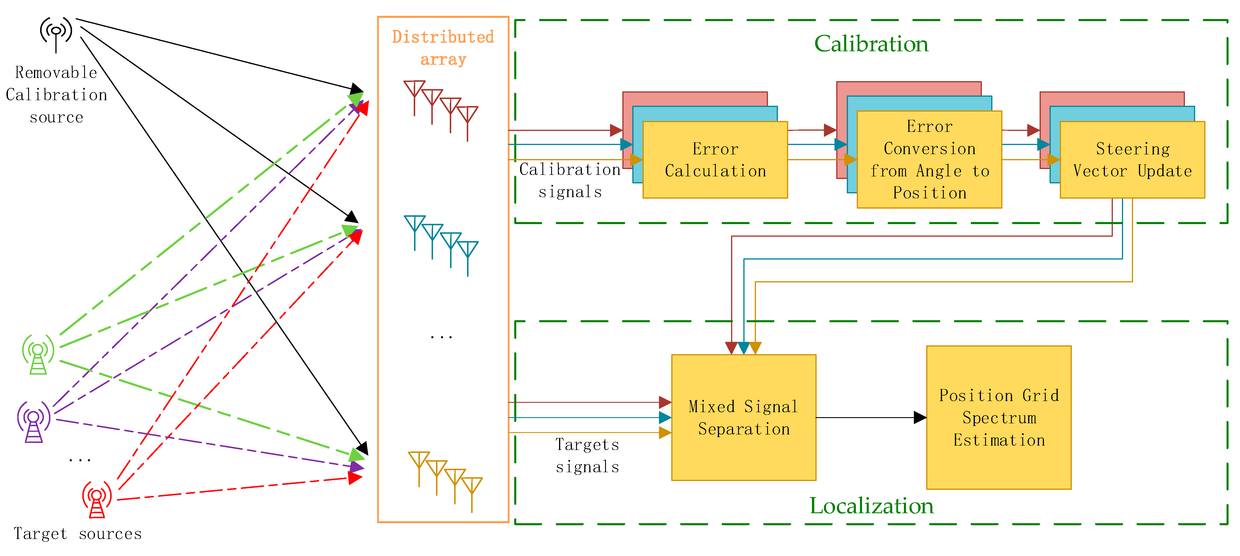
To address the challenge of target localization under complex amplitude–phase error conditions, this paper proposes an error calibration algorithm integrated with the EM 1-step method, forming a comprehensive system. The system is divided into two main components: error calibration and direct localization.
The error calibration component focuses on computing error matrices for different angles and their conversion to corresponding positions, as well as correcting the steering vector. The first task in this component involves calculating the amplitude–phase error matrix for various angles by receiving calibration signals from known positions and determining the deviations relative to simulated signals. These computed errors represent the amplitude–phase deviations for each angle of the array elements at each substation, forming the basis for signal separation. Subsequently, these errors are converted from different angles to different positions. This step calculates the errors corresponding to each position in the search grid and corrects the steering vector, which is essential for accurate energy spectrum computation.
The direct localization component uses the steering vector updated during error calibration to perform localization. The process begins by separating the received multi-target mixed signals into independent signals, each corresponding to a distinct target. Then, using the updated steering vector, the energy spectrum is calculated for each position in the search grid on the xy-plane. The peaks in the energy spectrum indicate the estimated positions of the targets.
For clarity, the typical Localization flow of the distributed array is illustrated in Figure 3. Detailed algorithms and processes for both components are elaborated in Section 3.2 and Section 3.3.
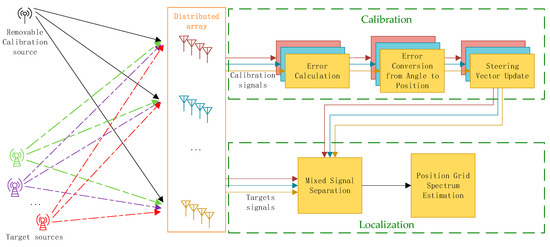
Figure 3.
The typical Localization flow of a distributed array.
3.2. Multi-Station Azimuth-Based Position Error Calibration Algorithm (MAPEC)
3.2.1. Calculation of Amplitude–Phase Error Matrix of Each Station
We designed a process to first measure the signals received from calibration sources with known azimuth angles at each station. By calculating the difference between the actual received signal at each antenna and the expected signal, the amplitude–phase error corresponding to each angle is obtained. The specific calculation method is as follows:
For the lth station, we place the calibration sources at distinct angles, denoted as . These angles are carefully selected to cover the desired calibration range. The signal received by the array is subjected to Fourier transform. The maximum value after transformation corresponds to the received signal frequency . The value corresponding to the received signal frequency calculates the amplitude–phase error. When the calibration source transmits the signal at of the lth station, the signal received by the mth antenna of the array is . The maximum value of the signal after the Fourier change contains the amplitude–phase information of the signal:
where is the amplitude of the received signal and is the phase.
In the simulation, a noise-free signal , originating from and received by the same antenna at the same station, is generated. This serves as the ideal reference signal for subsequent error calculations.
The amplitude difference and phase difference between the real signal and the simulation signal can be calculated as:
where represents the amplitude error of the signal from direction received by the mth antenna at the mth station, represents the phase error. Combining (16)–(19), the corrected array steering vector can be obtained.
However, direct localization requires searching in the location search grid. Therefore, the amplitude–phase error matrix needs to be transformed from different angles to different positions through scatter interpolation, obtaining the corrected array manifold .
3.2.2. Conversion of Amplitude–Phase Errors from Different Angles to Different Positions
This paper uses biharmonic spline surface interpolation to fit the amplitude–phase error calibration values extracted near the search grid points of interest, thus fitting the amplitude–phase error calibration values at all points of interest within the search grid. The principle of biharmonic interpolation is to calculate Green’s functions of the center points from the given data points, and the linear combination of these functions forms the interpolated surface. The surface generated by this method has minimal curvature.
The solution to the biharmonic equation is directly tied to Green’s function, which mathematically represents the response of the system to a point source. This concept has been widely applied in mechanics, physics, geology, and thermodynamics to model propagation phenomena. However, in the context of DOA estimation, this paper is the first to apply it to the construction of amplitude–phase error distributions across planar positions. By incorporating Green’s function into the interpolation, the algorithm effectively reconstructs a smooth and continuous error surface, providing accurate error estimates even in regions between sampled data points.
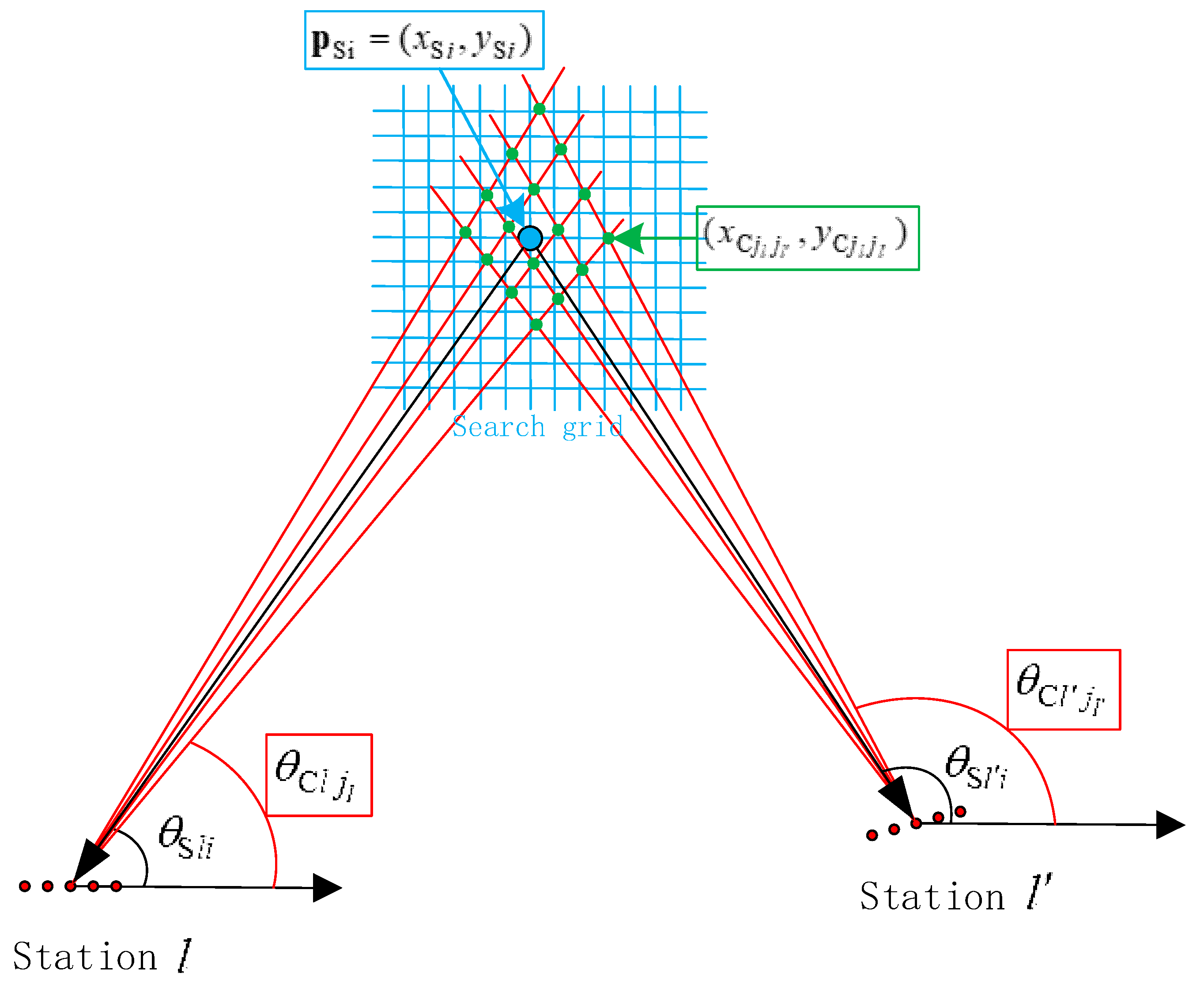
A theoretical model is shown in Figure 4. In the figure, the blue grid represents the search grid used for localization, with the defined area indicating the search range. The amplitude–phase errors corresponding to all grid points within the blue grid must be calculated in order to update the steering vector and achieve accurate localization. Specifically, one grid point (blue dot) will be selected as an example, and the error conversion calculation method for that point will be explained in detail. Suppose the coordinates of the blue dot are . The angle between the line connecting the point and the center antenna of each station (the blue line segments in Figure 4) and the positive direction of the x-axis is calculated as
where represents the x-axis coordinate of the center antenna of the lth station, and represents its y-axis coordinate.
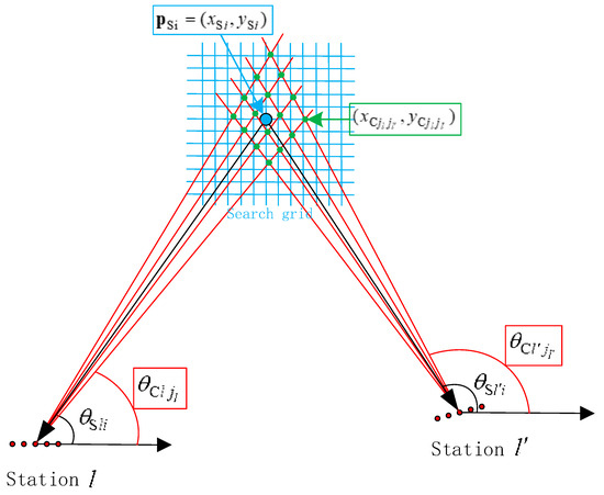
Figure 4.
A theoretical model for calculating the error coefficient of Station at the blue dot.
Find angle values in that are closest to , denoted as , . ensures that the data points used for interpolation are not overly sparse, which could otherwise result in insufficient parameters for the biharmonic interpolation algorithm. This sparsity would lead to interpolation results that deviate significantly from the actual values. Find angle values in closest to , denoted as . The biharmonic interpolation algorithm requires that the known interpolation points (green points in Figure 4) are distributed around the point of interest (blue points in Figure 4) rather than being located on only one side. Therefore, we specify , so as to achieve accurate interpolation. Using the center antenna of the station as the endpoint, draw rays with angles relative to the positive direction of the x-axis (the red rays in Figure 4). Different substation rays formed intersections (the green dots in Figure 4) near the blue dots. The total number of intersections formed by rays with the lth station as the endpoint and the rays with the th station as the endpoint is . The intersection positions for the rays from subarray with angle and rays from subarray with angle are
The amplitude–phase error coefficient , which exists when the signal at the intersection position is received by the mth antenna in the lth station, is obtained when the active calibration of each station is introduced above. For convenience, the position information and the amplitude–phase error information of the gth intersection are simplified denoted as , where , , , .
The distance between and in the xy-plane is calculated as
According to [31,32], the biharmonic equation can accurately estimate the value of a point at any location in the region between a bunch of sample data points. The established equation is as follows:
The surface fitting adopted in this paper uses 2D plane coordinates, so Green’s function uses . A key component of the biharmonic interpolation process is the use of the Green’s function, which plays a crucial role in describing how a localized “source” at a specific point propagates its influence across the surface. In the context of the interpolation, Green’s function serves as a mathematical tool to model the spreading of influence from a point source to the surrounding area. The function quantifies the smooth diffusion of the error’s effect, ensuring a continuous and physically realistic representation of the surface. The distance matrix can be established as
The distance matrix is symmetric, and its diagonal elements are 0. We can calculate the weight vector through , where . Then, the amplitude–phase error at the position point corresponding to the mth antenna at the lth station can be calculated as
where
Therefore, we can obtain the array manifold corrected by amplitude and phase error.
To make it clear, the proposed method MAPEC is summarized in Algorithm 1.
| Algorithm 1 Multi-Station Azimuth-based Position Error Calibration Algorithm |
| 1: for l = 1,2, …, L do 2: for m = 1,2, …, M do 3: for q = 1,2, …, Q do 4: The calibration source signal is transmitted at the azimuth of the Mth array element at the Lth station, The signal received from the correction source is ; 5: Simulated signal from without error; 6: Calculate the amplitude–phase information of real signal and simulated signal by (20)–(23); 7: Calculate the amplitude–phase error by (24)–(26) 8: end for 9: end for 10: end for 11: for i = 1, 2, …, I do 12: Find multiple points near where the exact error value is known, and their coordinates are calculated by (29); 13: Calculate the distance to of the points with known error values by (30); 14: Establish biharmonic equation by (31); 15: Calculate the error value by (33); 16: end for 17: Update array manifold by (36). |
3.3. EM-Based 1-Step Localization Algorithm
3.3.1. Signal Separation Using Updated Steering Vector
We apply the EM-based 1-step technique [29] to solve the optimization problem by an iteration strategy. Consider the received data (i.e., the incomplete data) as the mixture of independent Gaussian vectors , which can be expressed as
Before localization, the received multi-target mixed signals at each substation must first be decomposed into N individual signals using the EM algorithm. To successfully separate these N signals, the number of array elements, M, must satisfy the condition M > N. This ensures sufficient degrees of freedom for effective signal decomposition and accurate localization.
Let denote the estimate of the ith iteration, and we give the procedures of the EM algorithm as follows:
E-step:
M-step:
is the estimate of the incident wave direction angle of the nth emitter estimated by the lth station of the ith iteration. is obtained by running the E-step and M-step alternately until the algorithm converges. is the matrix containing all angles of the angle search grid, , where is the total number of search angles. To make the calculation easier, let’s set here. Thus, when , . And is solved in (28).
3.3.2. Position Estimation via Energy Spectrum Calculation
Once the signals have been separated, the next step involves localizing each of the N isolated single-target signals independently. This ensures that accurate localization results are obtained for each target.
Unlike the 2-step methods, the 1-step localization algorithm does not directly use the angle estimate for localization. By utilizing the estimated covariance matrix of the complete data the estimated position of emitters are located according to
which can be solved by applying a 2D search. represent all the predefined search points within the pre-search area for direct localization. Each search grid point is denoted by , where is the total number of search grid points in the xy-plane. The specific values of the search area and search grid depend on the experimental setup and context. At this stage, the received signals have already been decomposed into multiple independent signals, and single-target localization requires at least two stations to function effectively. Therefore, needs to be greater than or equal to 2.
4. Simulation Results
4.1. Analysis of Geometric Dilution of Precision (GDOP) in Distributed Arrays
This section investigates the GDOP in a distributed array localization system. To simplify the analysis, two uniform linear arrays (ULAs) are employed, positioned along the x-axis with a baseline length of . The subsections explore the effects of array configurations and error parameters on the GDOP performance. This section investigates the GDOP in a distributed array localization system. To simplify the analysis, two uniform linear arrays (ULAs) are employed, positioned along the x-axis with a baseline length of , which refers to the straight-line distance between the centers of the two station arrays. The subsections explore the effects of array configurations and error parameters on the GDOP performance.
4.1.1. The Calculation Formula of GODP
GDOP quantifies the influence of sensor array geometry on localization accuracy. For angle-of-arrival (AOA) systems, GDOP depends on the relative positions of sensor arrays and the target, as well as the angular estimation error. A lower GDOP corresponds to higher localization accuracy, making it an essential metric in designing distributed array systems.
In this study, ULAs are chosen for their simplicity and ease of deployment. The application scenario involves detecting targets on the sea surface, where it is unnecessary to monitor inland directions or estimate elevation angles. These requirements align well with the azimuthal coverage and one-dimensional structure of ULAs.
The angular estimation error for a ULA varies across azimuth angles, forming a U-shaped curve. The error is minimal at 90° due to the array’s optimal sensitivity and maximal at 0° and 180°. To model this, we define the angular error as
where is the minimum angular error at 90°. This model captures the anisotropic angular error distribution characteristic of ULAs.
The GDOP formula used in this analysis is derived from [33] and expressed as
where is the Jacobian matrix of the measurement model, and is the angular error covariance matrix constructed using .
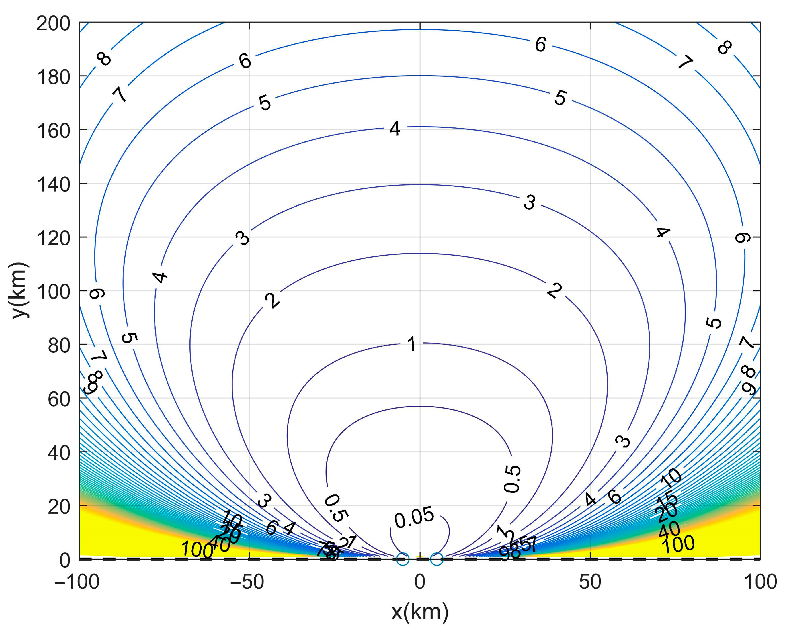
By substituting the error model into this equation, we simulate GDOP for two ULAs placed along the x-axis, separated by a baseline length km. The two blue circles at (±5, 0) km in Figure 5 are the centers of the two stations. And the distance between the two blue circles is baseline length .
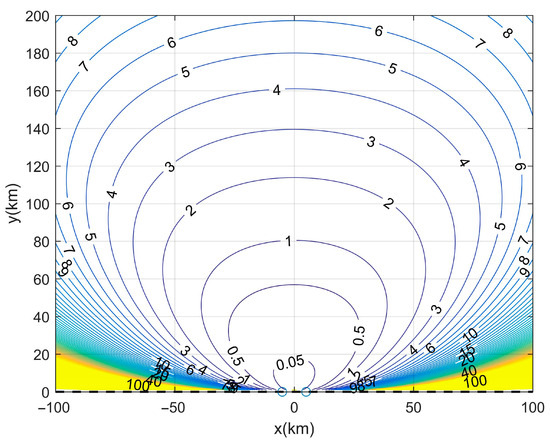
Figure 5.
GDOP distribution across the xy-plane for km and = 0.05°.
In Figure 5, the GDOP values are visualized for different target positions, highlighting the spatial variation in localization precision. Different colored lines on the figure indicate different GDOP values. Specifically, the closer the line is to blue, the smaller the GDOP value of each position on it, and the closer the line is to yellow, the larger the GDOP value. It can be observed that, due to the varying angle estimation errors of the ULA at different directions, the GDOP contours in the xy-plane do not form a perfect circle but instead resemble an inverted chestnut shape. Additionally, the farther the location is from the two stations, the denser the GDOP contours become.
4.1.2. Influence of Array Intersection Angle on GDOP
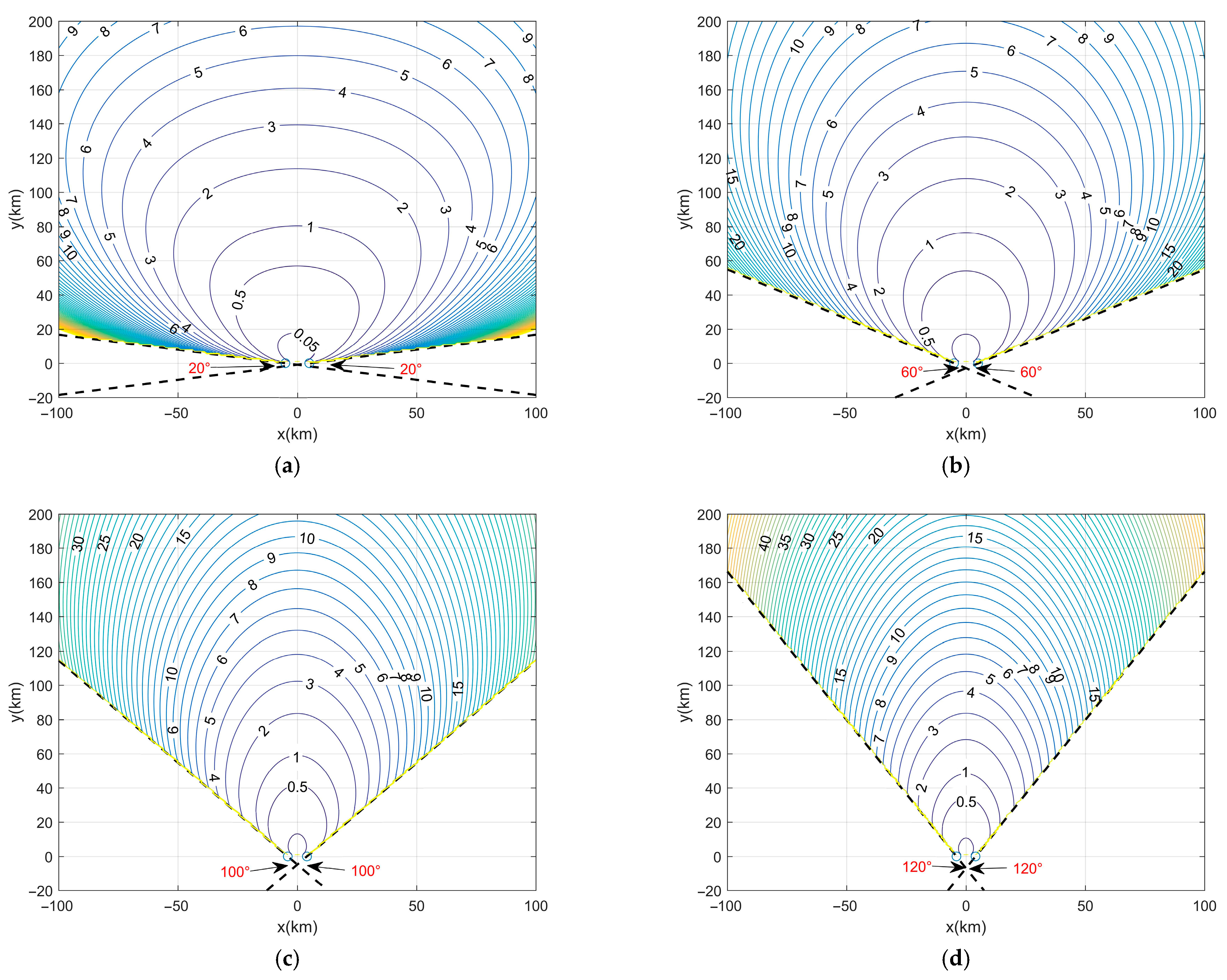
In Figure 6, the black dashed line is the array extension line of the two subarrays. The red angle specially marked at their intersection is the array intersection angle. Figure 6 depicts the GDOP distributions for four different intersection angles. The different colors of the lines in the figure have the same meaning as the colors of the lines in Figure 5.
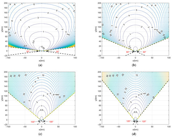
Figure 6.
GDOP distribution for D = 10 km and = 0.05° with different array intersection angles. (a) Array intersection angle is 20°. (b) Array intersection angle is 60°. (c) Array intersection angle is 100°. (d) Array intersection angle is 120°.
The intersection angle, defined as the angle formed at the intersection of the two array extension lines, plays a critical role in determining the GDOP distribution and the size of the detectable region. For ULAs, which only provide coverage within 0–180°, the alignment of the arrays heavily influences localization performance. The detection region should avoid crossing the array extension lines, as shown by the black dashed lines in Figure 6a–d, since localization accuracy in these areas is significantly degraded. When the arrays are parallel (0°), as shown in Figure 5, the detectable region is at its largest. However, as the intersection angle increases, the detectable region becomes narrower, and the GDOP precision at the same location points decreases. Additionally, because angular estimation errors are minimal near the normal directions of the ULAs and highest along the array extension lines, the GDOP contours take on the shape of an ellipse that is elongated vertically and narrowed on the sides, rather than a perfect circle. This means that, at the same distance, points closer to the normal directions of the arrays have smaller GDOP values and thus higher localization precision. Therefore, for a given detection area, aligning the target region closer to the normal directions of the arrays is beneficial.
4.1.3. Effect of Angular Error and Baseline Length on GDOP
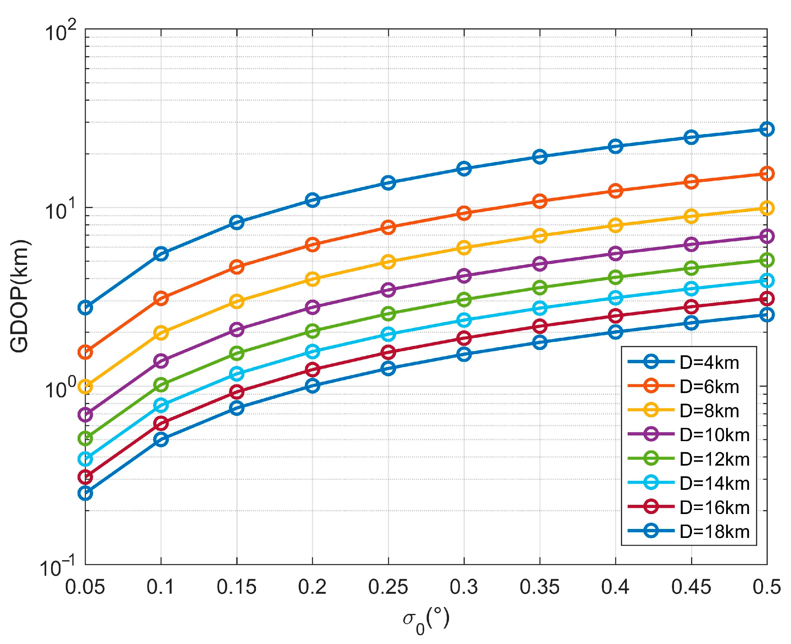
To evaluate the combined effects of angular error and baseline length , we consider various from 0° to 0.1° and values ranging from 4 km to 20 km. Figure 7 illustrates the variation of GDOP at the specific location (0, 100) km on the xy plane, with different and different .
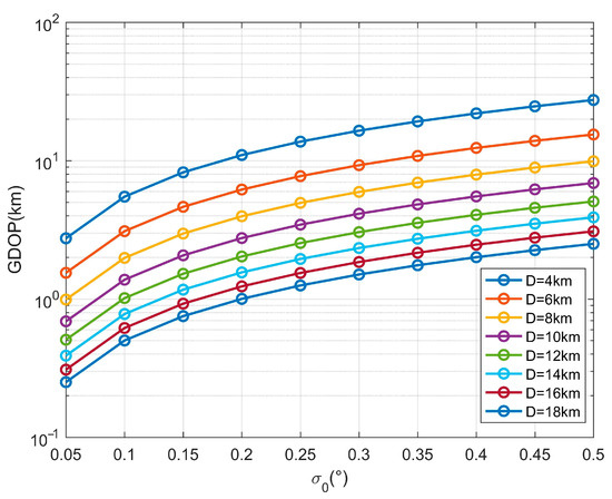
Figure 7.
GDOP variation with baseline length under different angular errors.
Based on Figure 5, the results reveal a clear relationship between baseline length and GDOP under varying angular error. As the baseline length increases, the GDOP decreases for all angular error levels, indicating improved localization accuracy with larger inter-station distances. However, the impact of angular error becomes more pronounced as increases, leading to a gradual rise in GDOP values across all . Notably, for larger baseline lengths, the GDOP demonstrates greater robustness to increases in angular error, while shorter baseline lengths are more sensitive to angular error variations. This highlights the importance of optimizing baseline length to mitigate the effects of angular error and improve overall localization precision.
4.2. Usability Simulation of the Proposed Algorithm
To closely simulate a realistic antenna signal reception environment with mixed errors, this section models amplitude and phase errors for each antenna element independently. We define the incident angle as the angle between the direction of the incoming wave and the positive X-axis. The amplitude error is generated by creating values at intervals of 20° from 0° to 180°, where these values follow a Gaussian distribution with a mean of 1, a maximum of 1.5, and a minimum of 0.5. During the interpolation phase, values are generated every 0.001° to ensure smooth and continuous variation of the amplitude error across angles. Similarly, the phase error is generated by creating values every 20° within the same angular range, following a Gaussian distribution with a mean of 0 and ranging from −π/4 to π/4, which are also smoothly interpolated. This process results in two smooth, continuous error matrices that vary irregularly with angles, effectively simulating the complex and unpredictable error environment encountered in practical scenarios. In (20), the combined amplitude–phase error is defined as . These assumptions allow us to mimic practical scenarios where signal reception is affected by multiple, angle-dependent error sources.
In the active calibration process, known position sources are utilized to measure the amplitude and phase errors at each station. This calibration is conducted across a search range of 0° to 180° with measurements taken at intervals of 10°. By performing these measurements, an amplitude and phase error matrix is constructed for each antenna at various angles. This error matrix serves as a critical input for the subsequent localization process, enabling the effective calibration of errors that could adversely affect the accuracy of the localization results.
In this section, calibration sources with known positions are utilized to measure the errors for each antenna across a search range from 0° to 180°, with a calibration measurement step size of 1°. Then, the algorithm proposed in this paper is used to convert the error matrix at each station from different angles to different positions. After the calibration is applied, a 1-step direct localization algorithm can be employed to accurately determine the target position.
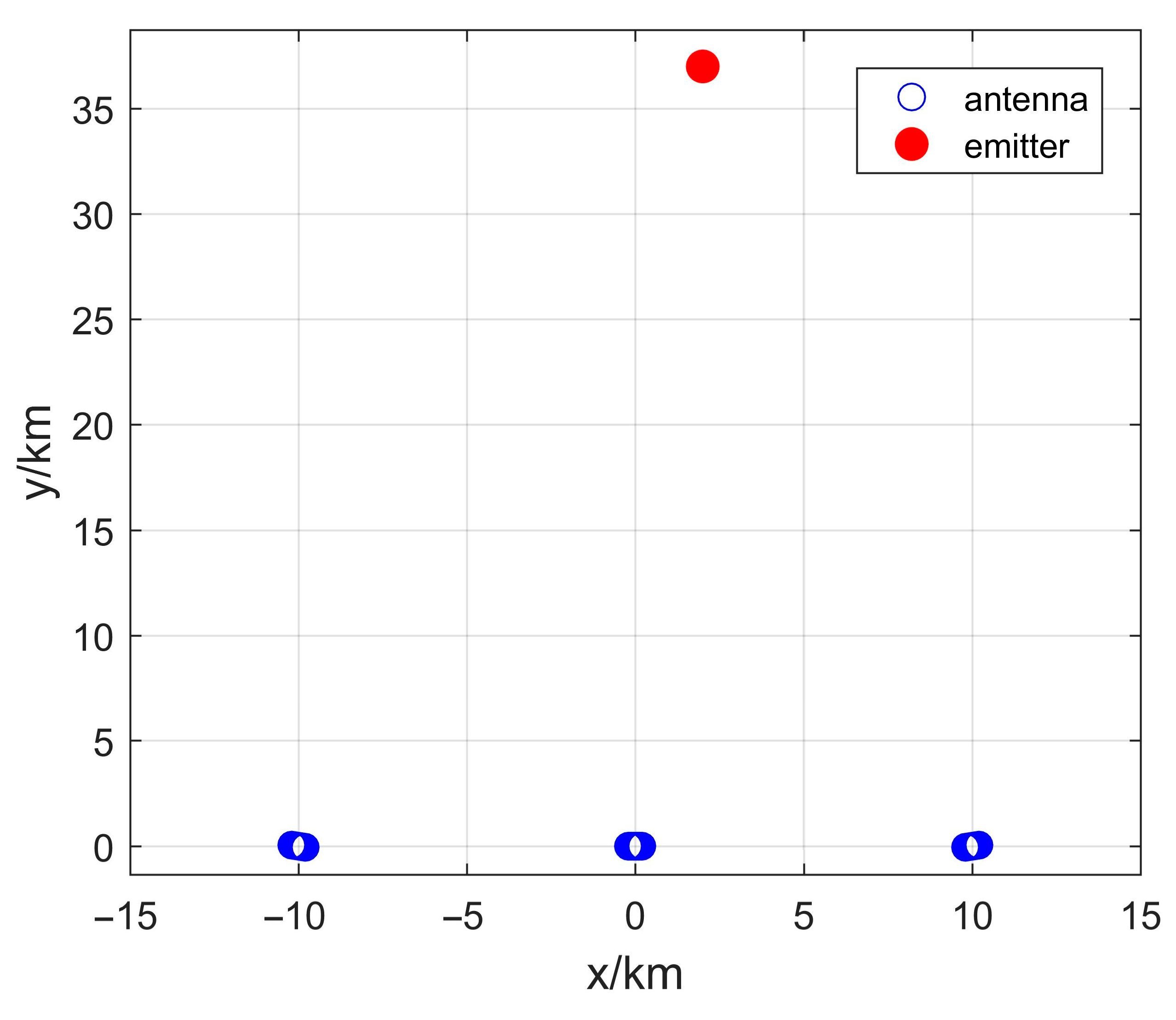
In our simulation, we consider a detection environment near a straight coastline, where the objective is to detect and locate emission sources originating from the sea. Given this setting, each station employs a simple linear array to cover a detection range from 0° to 180° effectively. Figure 8 illustrates the xy-planar layout, showing the positions and orientations of the stations and emitters. The three stations (Station 1, Station 2, and Station 3) are linearly arranged along the X-axis, with a distance of between each adjacent pair of stations. In this section, is set to 10 km. Each station is equipped with a uniform linear array (ULA) consisting of 10 antennas, with an antenna spacing of 0.05 km. The normal (perpendicular) direction of Station 2 is aligned parallel to the Y-axis, which is considered as 0°, while the normal directions of Stations 1 and 3 are oriented at +10° and −10°, respectively, relative to the positive Y-axis. Assuming there is one emitter located at (2,37) km, SNR is 0 dB and SNAP is 1000. The search area is (1 to 3, 32 to 42) km, the step size is 0.005 km. Thus, the search grid is set as [−1:0.05:3, 32:0.05:42] km.

Figure 8.
The xy-planar graph of the position diagram of the antenna arrays and emitters.
Figure 9 depicts the spatial spectrum obtained by the 1-step direct localization algorithm in the absence of amplitude–phase errors and without calibration. The spectrum shows a well-defined peak at (2, 37.05) km, which is very close to the actual emitter location (2, 37) km. The minor localization error indicates high localization accuracy under error-free conditions. Figure 10 presents the spatial spectrum of the 1-step direct localization algorithm with amplitude–phase errors but without applying any calibration. Here, the spectral peak shifts significantly, with the maximum energy deviating from the actual emitter location. The spectrum also appears highly distorted, demonstrating that uncorrected amplitude–phase errors severely impact localization performance. Figure 11 illustrates the spatial spectrum of the 1-step direct localization algorithm after applying the proposed amplitude–phase error calibration algorithm. Here, the spectral peak is located at (2, 36.9) km, which is close to the true emitter position. Compared to the uncorrected scenario in Figure 10, the spectrum in Figure 11 is significantly improved, with the spectral peak much sharper and closer to the true location.
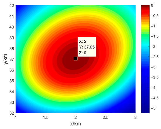
Figure 9.
Spatial Spectrum of 1-Step Localization Algorithm Without Errors and Without Calibration.
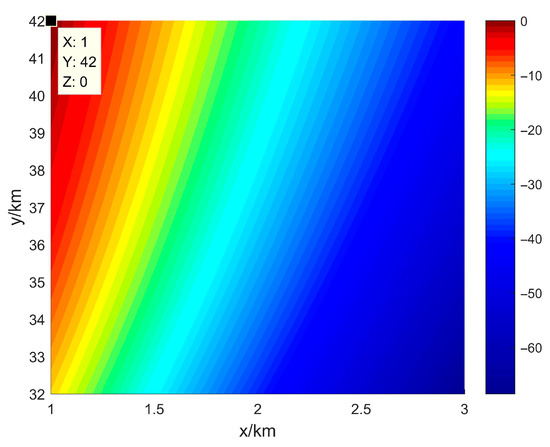
Figure 10.
Spatial Spectrum of 1-Step Localization Algorithm with Errors and Without Calibration.
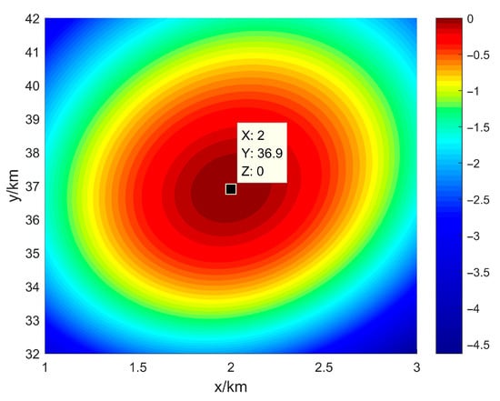
Figure 11.
Spatial Spectrum of 1-Step Localization Algorithm with Errors and Calibration Using the Proposed Method.
The comparison of Figure 9, Figure 10 and Figure 11 demonstrates that the proposed calibration algorithm effectively addresses the issue of localization failure in the presence of complex amplitude–phase errors. By mitigating the impact of these errors, the algorithm enables the 1-step localization method to accurately identify the emitter position with performance approaching that of the error-free environment. This validates the robustness and precision of the proposed approach in challenging error conditions.
4.3. Comparative Simulation Results
The localization accuracy is evaluated in terms of RMSE from Monte Carlo trials to demonstrate the DOA estimation performance further. The RMSE is defined as
where denotes the localization estimate of the nth emitter in the qth Monte Carlo trial, and is the nth emitter ’s true position. Set in the simulations.
In the comparison of the proposed calibration method MAPEC, we also present the simulation results of four 2-step algorithms (MUSIC [25], EM [26], FB-MUSIC [34], MVDR [35]) and another direct location algorithm (Wax’s algorithms [30]). The purpose of this comparison is to evaluate the performance of our proposed error calibration algorithm that can be applied to some location algorithms. In the presence of amplitude–phase errors, all 2-step algorithms in the simulation first proactively calibrate and estimate DOA at each site using the traditional active calibration algorithm based on multiple known reference signals, and then perform cross-positioning to obtain location information. Wax’s algorithm, like the 1-step algorithm mentioned in Section 3.2, is a direct localization algorithm. Therefore, the proposed MAPEC in Section 3.3 is equally applicable to Wax’s algorithm under such error conditions.
The settings of distributed array configuration, active calibration source, and error generation model in this section are consistent with those in Section 4.2.
4.3.1. RMSE vs. Amplitude–Phase Error Magnitude
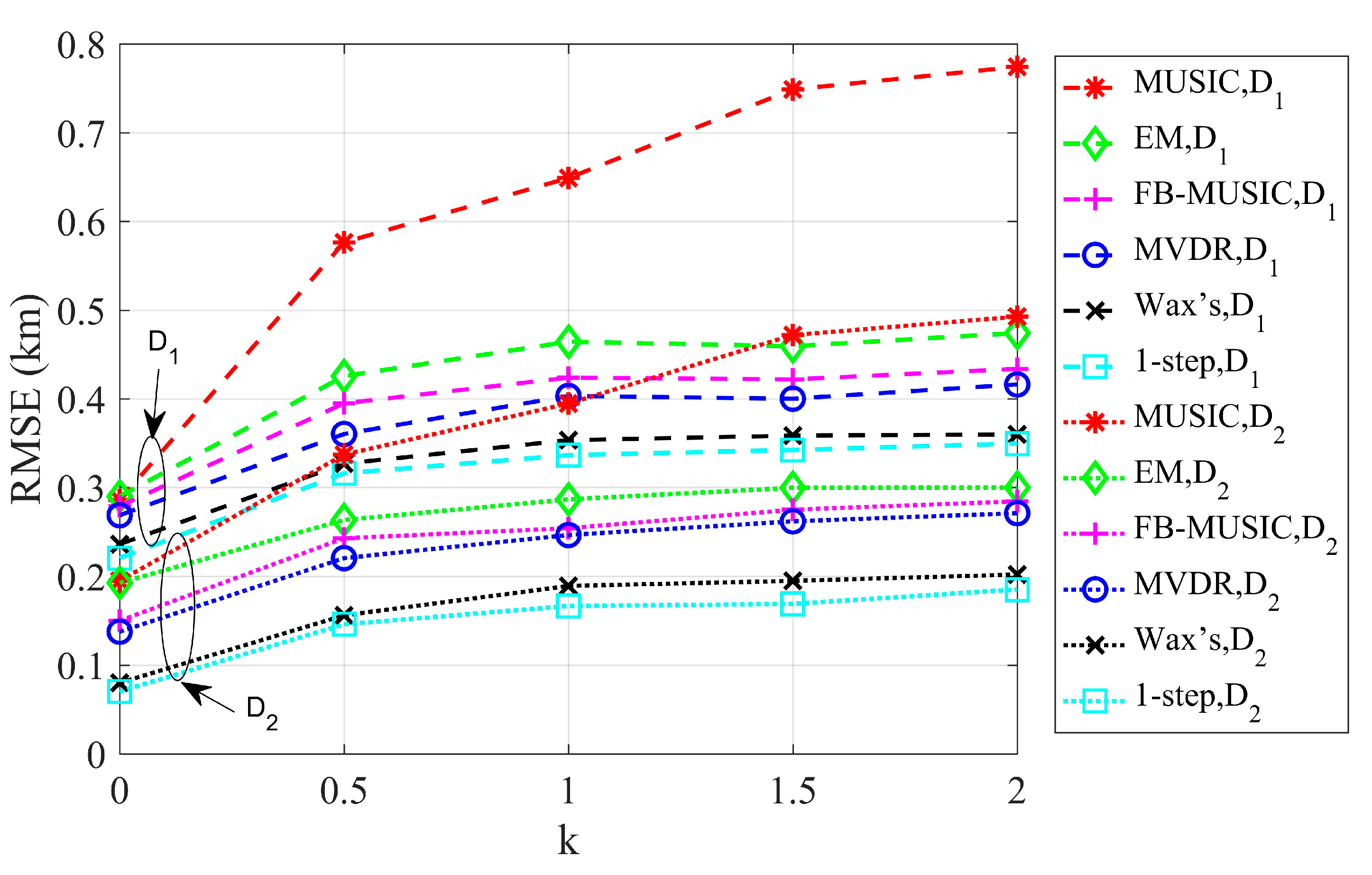
Figure 12 presents the RMSE performance of different positioning algorithms and calibration methods as the error size, denoted by the constant , varies. emitters located at (−10, 25) km and (10, 35) km, transmit uncorrelated random HF signals at a frequency of 3 MHz. SNR is set as 10 dB, SNAP is set as 1000. The search angle of each station with the 2-step method is (0~180)°, and the step size is 10−5°. The search area is (−20 to 20, 15 to 45) km, the step size is 0.005 km. Thus, the search grid is set as [−20:0.05:20, 15:0.05:45] km. The serves as a scaling factor for the amplitude–phase error matrices, . Recall that the amplitude–phase error is defined as , where and are matrices generated to vary smoothly and randomly with angle. In this experiment, while and are generated in the same manner as before, the error is redefined as , amplifying the original errors proportionally to .
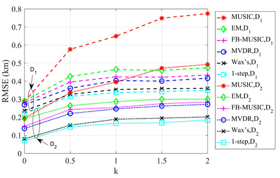
Figure 12.
RMSE with different error sizes under different positioning algorithms and calibration algorithms.
In Figure 12, we performed simulations for two scenarios with different subarray spacings ( km and km). The results show that localization performance improves with larger . Moreover, the RMSE trends of the six algorithms remain consistent for both values as increases. Specifically, as grows, the RMSE of all six algorithms increases correspondingly. Among them, the 2-step FB-MUSIC algorithm exhibits the most pronounced increase in RMSE with k, performing the worst after error calibration. This is because active calibration alters the array’s steering vectors, and the FB-MUSIC algorithm’s strong dependence on array configuration results in suboptimal performance after calibration.
The direct localization algorithms outperform the 2-step localization algorithms regardless of the presence of errors. The 1-step algorithm consistently delivers the best performance across different k values. Although RMSE increases with , the growth rate gradually diminishes, and once k reaches a certain level, the RMSE differences among the algorithms, except FB-MUSIC, become negligible.
Based on Figure 12, we conclude that the proposed calibration method effectively addresses the challenges posed by complex amplitude–phase errors in direct localization scenarios. Despite increasing error severity, the direct localization algorithms consistently demonstrate superior performance compared to traditional 2-step algorithms, achieving more accurate target localization. This highlights the robustness and precision of the proposed approach, making it a valuable solution for correcting direct localization algorithms in environments with significant and unpredictable amplitude–phase errors.
4.3.2. RMSE vs. SNR
Figure 13 shows the RMSE vs. SNR for different location and calibration algorithms, emitters located at (−10, 25) km and (10, 35) km, transmit uncorrelated random HF signals at a frequency of 3 MHz. The signals sent by the two emitters are independent. The SNAP is set as 1000. The search angle of each station with the 2-step method is (0~180)°, and the step size is 10−5°. The search grid of 1-step and Wax’s direct localization is [−20:0.05:20, 15:0.05:45] km. SNR is the variable in this set of experiments, which is set as [0:5:15] dB. Complex amplitude–phase errors exist in the simulation experiments in this section, and the generation method is consistent with the generation error method in 4.2.
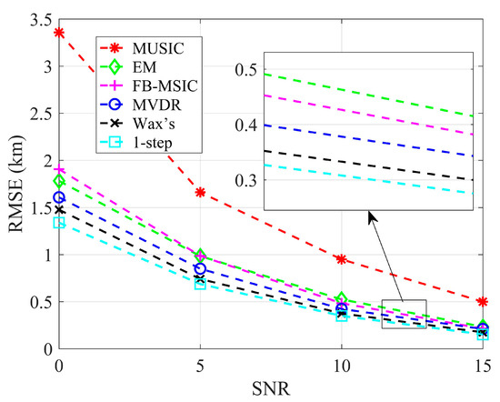
Figure 13.
RMSE with different SNR under different positioning algorithms and calibration algorithms.
Figure 13 illustrates the impact of SNR on the localization performance of various algorithms. In the presence of complex amplitude–phase errors and after calibration, the 2-step EM algorithm achieves the best performance among the 2-step algorithms. However, its performance remains inferior to the direct localization algorithms. The performances of 2-step MVDR and 2-step MUSIC are comparable, with MVDR slightly underperforming at low SNR but surpassing MUSIC at high SNR. The performance of 2-step FB-MUSIC significantly deteriorates after error calibration, primarily due to its strong dependence on the array configuration, which is affected by active calibration. Among the direct localization algorithms, the 1-step algorithm consistently outperforms Wax’s algorithm, highlighting its superior accuracy. Overall, the proposed error calibration method effectively addresses the challenges posed by complex amplitude–phase errors, enabling the 1-step algorithm to retain its localization advantage across different SNR levels and maintain robustness in error-prone environments.
4.3.3. RMSE vs. SNAP
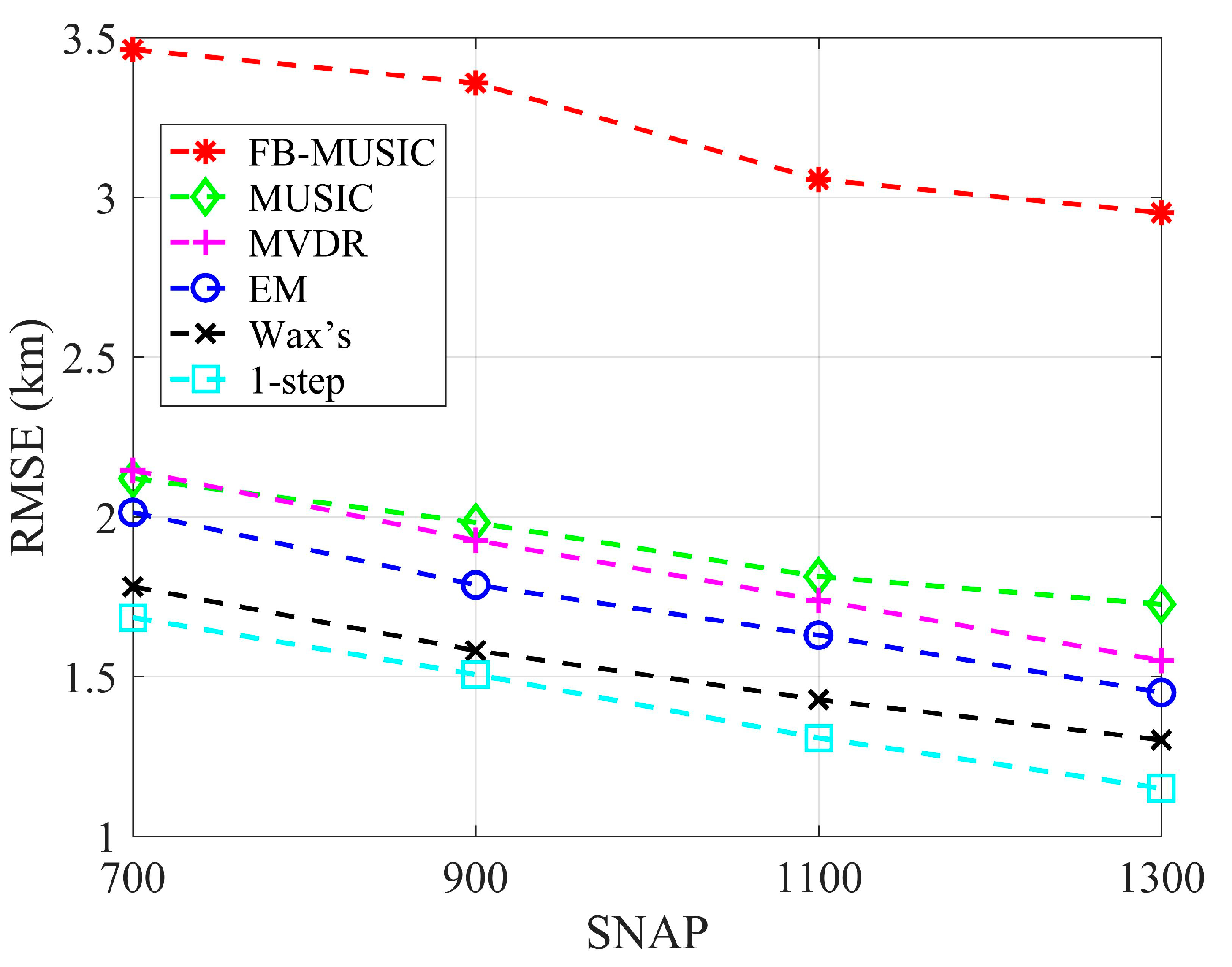
Figure 14 shows that the RMSE vs. SNAP for different locations and calibration algorithms, emitters located at (−10, 25) km and (10, 35) km, transmit uncorrelated random HF signals at a frequency of 3 MHz. The signals sent by the two emitters are independent. The SNR is set as 0 dB. The search angle of each station with the 2-step method is (0~180)°, and the step size is 10−5°. The search grid of 1-step and Wax’s direct localization is [−20:0.05:20, 15:0.05:45] km. SNAP is the variable in this set of experiments, which is set as [700:200:1300]. Complex amplitude–phase errors exist in the simulation experiments in this section, and the generation method is consistent with the generation error method in Section 4.2.

Figure 14.
RMSE with different SNAP under different positioning algorithms and calibration algorithms.
Figure 14 illustrates how the RMSE varies with the number of SNAP for different localization algorithms. The simulation results indicate that, as the number of snapshots increases, the RMSE decreases for all algorithms, demonstrating that localization performance improved with more data. Among the 2-step algorithms, the 2-step EM algorithm is the most stable, though it still lags behind the direct localization algorithms. These findings emphasize the robustness and accuracy of the proposed error calibration method, particularly for the 1-step algorithm in challenging error conditions. Regardless of the SNAP value, the proposed method ensures that the 1-step localization algorithm maintains its performance advantage, effectively enhancing its resilience in complex error environments.
4.3.4. RMSE vs. Distance Between Station and Emitter
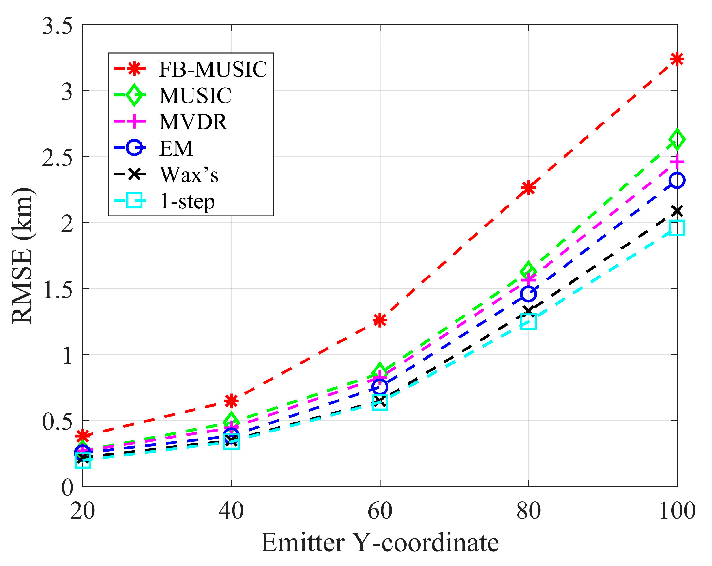
Figure 15 shows the RMSE vs. the distance between station and emitter for different locations and calibration algorithms. SNR is set as 0 dB, SNAP is set as 900. For a clearer comparison, only one emitter is emulated in this subsection, . The frequency of the signal is 3 MHz. The Y-coordinate of the emitter is the variable in this set of experiments, which is set as [20:20:100] km. The X-coordinate of emitter is set as 0 km. The search angle of each station with the 2-step method is still (0~180)°, and the search grid of 1-step and Wax’s direct localization is [−5:0.05:5, 15:0.05:105] km. Complex amplitude–phase errors exist in the simulation experiments in this section, and the generation method is consistent with the generation error method in Section 4.2.
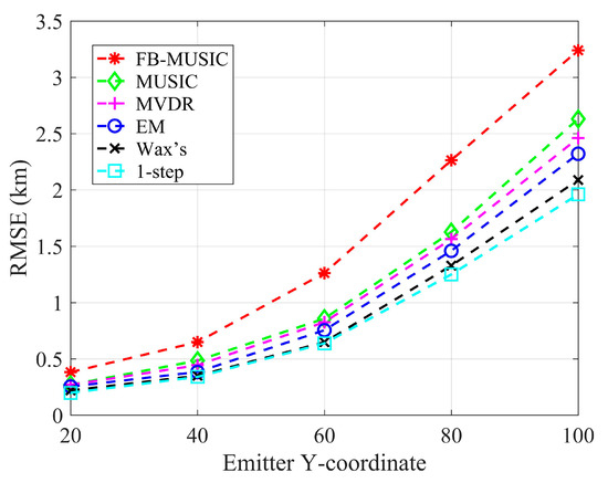
Figure 15.
RMSE with different distances of emitters under different positioning algorithms and calibration algorithms.
Figure 15 shows the impact of increasing emitter distance (Y-coordinate) on RMSE for different localization algorithms. As the emitter distance grows, the localization accuracy of all algorithms decreases, reflected in the rising RMSE trends.
The direct localization algorithms consistently achieve the lower RMSE compared to all 2-step algorithms, highlighting their inherent advantage in localization performance. The proposed error calibration method effectively resolves the challenges posed by complex amplitude–phase errors, enabling the 1-step algorithm to retain its superior accuracy, even under error conditions. Overall, the results demonstrate that the proposed calibration approach preserves the advantages of the 1-step localization algorithm, ensuring accurate localization in challenging error scenarios while outperforming traditional 2-step methods.
5. Conclusions and Discussion
In this paper, we propose a novel approach to correct amplitude–phase errors in direct localization of emitters within distributed multi-station systems. Unlike traditional global calibration methods that require intensive calibration efforts at each search grid position, our approach leverages a localized strategy. Specifically, active calibration is performed at each search angle for individual stations, substantially reducing the number of required calibration sources and increasing the practicality of the calibration process.
Our method integrates seamlessly with various direct localization algorithms that are based on direction-of-arrival (DOA) estimation, effectively addressing error calibration challenges in scenarios with complex amplitude–phase distortions. The simulation results demonstrate that our proposed algorithm consistently outperforms traditional 2-step methods like 2-step FB-MUSIC, 2-step MUSIC, 2-step MVDR, and 2-step EM, providing more accurate localization even under severe error conditions. Both Wax’s algorithm and our proposed 1-step method, using the new calibration strategy, deliver robust performance, with the 1-step approach showing particular effectiveness across varying signal-to-noise ratios (SNR), snapshot counts (SNAP), and emitter distances.
However, there are limitations that we need to address in future research. Specifically, our method cannot be applied if the underlying DOA algorithm imposes restrictions on array configurations, such as requiring all stations to be uniform linear arrays (ULAs). This restriction arises because the corrected array manifold matrix produced by our method cannot fulfill ULA-specific constraints. Exploring solutions to extend our approach to arrays with more flexible configurations is a critical area for future investigation.
Additionally, in this study, we focus on the theoretical and simulation-based validation of the proposed MAPEC algorithm, demonstrating its robustness and precision under various error conditions. While these results confirm the effectiveness of our approach, its application to real-world data remains an important future direction. At present, due to limitations in experimental resources, we have not yet conducted practical experiments or collected actual data to validate the algorithm. However, in future work, we aim to establish a distributed multi-station receiver platform to gather real-world data for testing and further refinement of the proposed method. Practical experiments will provide critical insights into the algorithm’s performance under realistic environmental and hardware conditions, ensuring its applicability in operational systems.
Author Contributions
Conceptualization, H.M.; Data curation, H.M.; Formal analysis, H.M.; Funding acquisition, X.M.; Methodology, H.M. and X.M.; Project administration, X.M.; Software, H.M.; Supervision, X.M.; Validation, H.M.; Visualization, H.M.; Writing—original draft, H.M. and X.M.; Writing—review and editing, H.M., X.M., Y.Q. and Y.G. All authors have read and agreed to the published version of the manuscript.
Funding
This research was supported by the Key Project of National Natural Science Foundation of China (No. 61831009), National Natural Science Foundation of China (No. 62371479), and the Aeronautical Science Foundation of China (No. 2024Z073077002).
Data Availability Statement
The original contributions presented in the study are included in the article, further inquiries can be directed to the corresponding author.
Conflicts of Interest
The authors declare no conflicts of interest.
References
- Chuang, L.Z.-H.; Chen, Y.-R.; Chung, Y.-J. Applying an Adaptive Signal Identification Method to Improve Vessel Echo Detection and Tracking for SeaSonde HF Radar. Remote Sens. 2021, 13, 2453. [Google Scholar] [CrossRef]
- Zhou, Q.; Bai, Y.; Zhu, X.; Wu, X.; Hong, H.; Ding, C.; Zhao, H. Spreading Sea Clutter Suppression for High-Frequency Hybrid Sky-Surface Wave Radar Using Orthogonal Projection in Spatial–Temporal-domain. Remote Sens. 2024, 16, 2470. [Google Scholar] [CrossRef]
- Corgnati, L.; Berta, M.; Kokkini, Z.; Mantovani, C.; Magaldi, M.G.; Molcard, A.; Griffa, A. Assessment of OMA Gap-Filling Performances for Multiple and Single Coastal HF Radar Systems: Validation with Drifter Data in the Ligurian Sea. Remote Sens. 2024, 16, 2458. [Google Scholar] [CrossRef]
- Wyatt, L.R.; Green, J.J. Developments in Scope and Availability of HF Radar Wave Measurements and Robust Evaluation of Their Accuracy. Remote Sens. 2023, 15, 5536. [Google Scholar] [CrossRef]
- Golubović, D.; Erić, M.; Vukmirović, N.; Orlić, V. High-Resolution Sea Surface Target Detection Using Bi-Frequency High-Frequency Surface Wave Radar. Remote Sens. 2024, 16, 3476. [Google Scholar] [CrossRef]
- Inoue, Y.; Mori, K.; Arai, H. DOA estimation in consideration of the array element pattern. In Proceedings of the Vehicular Technology Conference. IEEE 55th Vehicular Technology Conference. VTC Spring 2002 (Cat. No.02CH37367), Birmingham, AL, USA, 6–9 May 2002; Volume 2, pp. 745–748. [Google Scholar]
- Wang, D.; Zhang, F.; Chen, L.; Li, Z.; Yang, L. The Calibration Method of Multi-Channel Spatially Varying Amplitude-Phase Inconsistency Errors in Airborne Array TomoSAR. Remote Sens. 2023, 15, 3032. [Google Scholar] [CrossRef]
- Zhen, J.; Guo, B. DOA estimation for far-field sources in mixed signals with mutual coupling and gain-phase error array. J Wirel. Com Netw. 2018, 2018, 295. [Google Scholar] [CrossRef]
- Li, Z.; Huang, Z. Sparse Bayesian Learning Based DOA Estimation and Array Gain-Phase Error Self-Calibration. Prog. Electromagn. Res. M 2022, 108, 65–77. [Google Scholar] [CrossRef]
- Zhao, Z.; Tian, W.; Deng, Y.; Hu, C.; Zeng, T. Calibration Method of Array Errors for Wideband MIMO Imaging Radar Based on Multiple Prominent Targets. Remote Sens. 2021, 13, 2997. [Google Scholar] [CrossRef]
- Tian, Y.; Wang, X.; Ding, L.; Wang, X.; Feng, Q.; Zhang, Q. A New Sparse Bayesian Learning-Based Direction of Arrival Estimation Method with Array Position Errors. Mathematics 2024, 12, 545. [Google Scholar] [CrossRef]
- Yan, H.; Wang, Y.; Wang, L. Padded Sparse Array for DoA Estimation of Noncircular Signals in the Presence of Unknown Mutual Coupling. In Proceedings of the 2021 IEEE USNC-URSI Radio Science Meeting (Joint with AP-S Symposium), Singapore, 4–10 December 2021; pp. 114–115. [Google Scholar]
- Sebastian, J.; Dayal, P.; Song, K.-B.; AliAhmad, W. Explicit Calibration of mmWave Phased Arrays with Phase Dependent Errors. arXiv 2021, arXiv:2107.09561. [Google Scholar]
- Fu, W.; Liu, H.; Chen, Z.; Yang, S.; Hu, Y.; Wen, F. Improved Amplitude-Phase Calibration Method of Nonlinear Array for Wide-Beam High-Frequency Surface Wave Radar. Remote Sens. 2023, 15, 4405. [Google Scholar] [CrossRef]
- Lu, Z.; Jiang, H.; Gao, Y.; Shi, Y. Amplitude and phase errors self-correcting algorithm based on the uniform circular array. In Proceedings of the 2012 2nd International Conference on Computer Science and Network Technology, Changchun, China, 29–31 December 2012; pp. 136–140. [Google Scholar]
- Wang, C.; Tian, Y.; Yang, J.; Zhou, H.; Wen, B.; Hou, Y. A Practical Calibration Method of Linear UHF Yagi Arrays for Ship Target Detection Application. IEEE Access 2020, 8, 46472–46479. [Google Scholar] [CrossRef]
- Liu, S.; Zhang, Z.; Guo, Y. 2-D DOA Estimation With Imperfect L-Shaped Array Using Active Calibration. IEEE Commun. Lett. 2021, 25, 1178–1182. [Google Scholar] [CrossRef]
- Pan, C.; Ba, X.; Tang, Y.; Zhang, F.; Zhang, Y.; Wang, Z.; Fan, W. Phased Array Antenna Calibration Method Experimental Validation and Comparison. Electronics 2023, 12, 489. [Google Scholar] [CrossRef]
- Sarabandi, K.; Kashanianfard, M.; Nashashibi, A.Y.; Pierce, L.E.; Hampton, R. A Polarimetric Active Transponder With Extremely Large RCS for Absolute Radiometric Calibration of SMAP Radar. IEEE Trans. Geosci. Remote. Sens. 2018, 56, 1269–1277. [Google Scholar] [CrossRef]
- Reimann, J.; Büchner, A.M.; Raab, S.; Weidenhaupt, K.; Jirousek, M.; Schwerdt, M. Highly Accurate Radar Cross-Section and Transfer Function Measurement of a Digital Calibration Transponder without Known Reference—Part I: Measurement and Results. Remote Sens. 2023, 15, 1153. [Google Scholar] [CrossRef]
- Reimann, J.; Büchner, A.M.; Raab, S.; Weidenhaupt, K.; Jirousek, M.; Schwerdt, M. Highly Accurate Radar Cross-Section and Transfer Function Measurement of a Digital Calibration Transponder without Known Reference—Part II: Uncertainty Estimation and Validation. Remote Sens. 2023, 15, 2148. [Google Scholar] [CrossRef]
- Zhang, F.; Sun, Y.; Wan, Q. Calibrating the error from sensor position uncertainty in TDOA-AOA localization. Signal Process. 2020, 166, 107213, ISSN 0165-1684. [Google Scholar] [CrossRef]
- Kang, X.; Wang, D.; Shao, Y.; Ma, M.; Zhang, T. An Efficient Hybrid Multi-Station TDOA and Single-Station AOA Localization Method. IEEE Trans. Wirel. Commun. 2023, 22, 5657–5670. [Google Scholar] [CrossRef]
- Nyantakyi, I.O.; Wan, Q.; Ni, L.; Mensah, E.O.; Bamisile, O. ACGA: Adaptive Conjugate Gradient Algorithm for non-line-of-sight hybrid TDOA-AOA localization. Measurement 2024, 224, 113820, ISSN 0263-2241. [Google Scholar] [CrossRef]
- Schmidt, R. Multiple emitter location and signal parameter estimation. IEEE Trans. Antennas Propag. 1986, 34, 276–280. [Google Scholar] [CrossRef]
- Miller, M.I.; Fuhrmann, D.R. Maximum-likelihood narrow-band direction finding and the em algorithm. IEEE Trans. Acoust., Speech Signal Process. 1990, 38, 1560–1577. [Google Scholar] [CrossRef]
- Fan, W.; Liu, S.; Li, C.; Huang, Y. Fast Direct Localization for Millimeter Wave MIMO Systems via Deep ADMM Unfolding. IEEE Wirel. Commun. Lett. 2023, 12, 748–752. [Google Scholar] [CrossRef]
- Akbari, S.; Valaee, S. A Geometric Approach for Cooperative Direct Localization. In Proceedings of the 2023 IEEE 34th Annual International Symposium on Personal, Indoor and Mobile Radio Communications (PIMRC), Toronto, ON, Canada, 5–8 September 2023; pp. 1–6. [Google Scholar]
- Chen, M.; Mao, X.; Zhao, C. Direct localization of emitters based on expectation-maximization technique. In Proceedings of the 2018 IEEE Radar Conference (RadarConf18), Oklahoma City, OK, USA, 23–27 April 2018; pp. 0754–0758. [Google Scholar]
- Wax, M.; Kailath, T. Decentralized processing in sensor arrays. IEEE Trans. Acoust. Speech Signal Process. 1985, 33, 1123–1129. [Google Scholar] [CrossRef]
- Sandwell, D.T. Biharmonic spline interpolation of GEOS-3 and SEASAT altimeter data. Geophys. Res. Lett. 1987, 14, 139–142. [Google Scholar] [CrossRef]
- You, W.; Ding, Y.; Yao, Y. Static Explosion Field Reconstruction Based on the Improved Biharmonic Spline Interpolation. IEEE Sens. J. 2020, 20, 7235–7240. [Google Scholar]
- Torrieri, D.J. Statistical Theory of Passive Location Systems. IEEE Trans. Aerosp. Electron. Syst. 1984, 20, 183–197. [Google Scholar] [CrossRef]
- Yang, Z.; Stoica, P.; Tang, J. Source Resolvability of Spatial-Smoothing-Based Subspace Methods: A Hadamard Product Perspective. IEEE Trans. Signal Process. 2019, 67, 2543–2553. [Google Scholar]
- Capon, J. High-resolution frequency-wavenumber spectrum analysis. Proc. IEEE 1969, 57, 1408–1418. [Google Scholar] [CrossRef]


Disclaimer/Publisher’s Note: The statements, opinions and data contained in all publications are solely those of the individual author(s) and contributor(s) and not of MDPI and/or the editor(s). MDPI and/or the editor(s) disclaim responsibility for any injury to people or property resulting from any ideas, methods, instructions or products referred to in the content. |
© 2025 by the authors. Licensee MDPI, Basel, Switzerland. This article is an open access article distributed under the terms and conditions of the Creative Commons Attribution (CC BY) license (https://creativecommons.org/licenses/by/4.0/).