A Deep Learning-Based Method for Detection of Multiple Maneuvering Targets and Parameter Estimation

Abstract

With the rapid development of drone technology, target detection and estimation of radar parameters for maneuvering targets have become crucial. Drones, with their small radar cross-sections and high maneuverability, cause range migration (RM) and Doppler frequency migration (DFM), which complicate the use of traditional radar methods and reduce detection accuracy. Furthermore, the detection of multiple targets exacerbates the issue, as target interference complicates detection and impedes parameter estimation. To address this issue, this paper presents a method for high-resolution multi-drone target detection and parameter estimation based on the adjacent cross-correlation function (ACCF), fractional Fourier transform (FrFT), and deep learning techniques. The ACCF operation is first utilized to eliminate RM and reduce the higher-order components of DFM. Subsequently, the FrFT is applied to achieve coherent integration and enhance energy concentration. Additionally, a convolutional neural network (CNN) is employed to address issues of spectral overlap in multi-target FrFT processing, further improving resolution and detection performance. Experimental results demonstrate that the proposed method significantly outperforms existing approaches in probability of detection and accuracy of parameter estimation for multiple maneuvering targets, underscoring its strong potential for practical applications.

1. Introduction

With the rapid advancement of drone technology, radar detection and parameter estimation for drone targets has emerged as a critical research area in radar-signal processing. Drones are characterized by a low radar cross-section (RCS) and high maneuverability. Specifically, in complex environments and under low signal-to-noise ratio (SNR) conditions, accurately detecting and estimating the motion parameters of targets has become one of the primary challenges in contemporary radar technology [1,2,3,4,5,6,7,8].

In the context of effectively addressing the detection challenges associated with highly maneuverable drone targets, long-time coherent integration (LTCI) has proven to be an effective method for enhancing SNR. However, as the maneuverability of drone targets has increased, their motion characteristics have induced increasingly complex effects, such as Doppler frequency migration (DFM) and range migration (RM). In particular, under the influence of high-order motion parameters, such as jerk, traditional signal-processing methods struggle to accurately identify targets in low-SNR environments, further increasing the difficulty and complexity of signal processing [9,10,11].

To address these challenges, methods for time-frequency analysis such as Wigner–Ville Distribution (WVD) [12], Radon–Ambiguity Function (RAF) [13,14], and Radon–Fourier Transform (RFT) [15,16,17] have been widely applied in target detection. One of these, WVD, significantly enhances detection capabilities in low-SNR environments by providing high time-frequency resolution. However, in multi-target scenarios, WVD is prone to cross-term interference, which undermines detection accuracy. In contrast, RAF and RFT enhance target signals under low-SNR conditions through signal transformation but remain limited by RM effects and the characteristics of the motion of highly maneuverable targets, showing poor adaptability in dynamic scenarios. To overcome these limitations, the Generalized Radon–Fourier Transform (GRFT) [18,19,20] was proposed based on RFT; it effectively addresses RM and DFM. However, GRFT requires searching in a multi-dimensional motion-parameter space, resulting in high computational complexity. Furthermore, GRFT is susceptible to blind-speed sidelobes, which can lead to false detections and performance degradation. Recent advancements that aim to mitigate these issues include the Full-Dimensional Partial-Search Generalized Radon–Fourier Transform (FSGRFT) [11], which reduces computational cost by employing a pretrained residual network for coarse estimation of range cells and motion-parameter subspaces. Additionally, for bistatic PRI agile radar systems, the NU-SCGRFT method [21] was developed to handle the challenges of RM, DFM, and scale effect, thereby improving integration and parameter-estimation performance for high-speed maneuvering targets. Despite these improvements, there remains a significant need for methods that can effectively balance integration performance with computational efficiency, especially when dealing with high-order motion parameters.

A signal-representation method based on the Lv distribution was proposed by [22]; it accurately characterizes linear frequency modulation (LFM) signals through central frequency and frequency-modulation rate. This method offers higher resolution and avoids cross-term interference. However, it has certain limitations in detecting frequency range and chirp rate. Several additional effective methods have also been proposed. The KT transform [23,24], for instance, achieves RM correction by resampling along the time axis, making it suitable for high-speed target detection. However, it lacks adequate compensation for DFM caused by acceleration. Another notable approach is the Time Reversal Transform (TRT) [25], which can correct higher-order RM effects without requiring parameter searches. Nevertheless, these methods often result in a loss of SNR, thereby limiting their ability to detect weak targets under low-SNR conditions.

The Fractional Fourier Transform (FrFT), as a specialized linear time-frequency analysis method, has demonstrated significant advantages in detecting linear frequency modulation (LFM) signals and has garnered considerable attention in recent years [26,27,28,29,30,31,32,33,34,35]. To the traditional Fourier transform, FrFT introduces a free parameter, the rotation angle, enabling superior time-frequency concentration while avoiding cross-term interference. When the optimal transformation angle is selected, the signal energy is highly concentrated and the FrFT spectrum exhibits an ideal impulse-like characteristic, significantly enhancing the accuracy of signal processing.

However, FrFT exhibits notable limitations in handling high-order motion parameters, such as jerk. Additionally, in detection scenarios involving multiple targets, it often struggles to distinguish different targets accurately due to spectrum overlapping, leading to false detections or missed detections.

To address these issues, this paper proposes a novel method that integrates the Adjacent Cross Correlation Function (ACCF), the Fractional Fourier Transform (FrFT), and a Convolutional Neural Network (CNN) to tackle the coherent integration challenges in the detection of multiple maneuvering targets and parameter estimation, with a particular focus on effectively estimating high-order motion parameters such as jerk. ACCF effectively eliminates RM and, by computing the higher-order autocorrelation characteristics of the target signal, reduces the order of the Doppler frequency [36,37]. This transforms complex high-order frequency migrations into low-order signals that are easier to process, thereby enabling FrFT to accurately detect and estimate high-order motion parameters like jerk with greater precision. Moreover, in multi-target scenarios, ACCF effectively reduces cross-term interference, providing a clearer and more reliable signal foundation for FrFT. Despite the improved detection performance of the ACCF–FrFT combination, spectrum overlap in FrFT under multi-target conditions can still reduce target resolution. To further address this challenge, this paper integrates a Convolutional Neural Network (CNN) into the ACCF–FrFT framework. The core advantage of a CNN lies in its ability to automatically learn hierarchical feature representations from data. This makes CNN particularly effective in tasks such as signal-parameter estimation, in which capturing complex patterns and local correlations is crucial. By learning signal features, CNN effectively mitigates the interference caused by spectrum overlap. The ACCF–FrFT method, enhanced with CNN, significantly improves the accuracy and robustness of the detection of multiple targets. Our contributions are threefold:

(1)

We utilized the ACCF method to process the DFM and RM of multi-target signals. This method effectively eliminates RM, reduces the order of DFM, and mitigates interference caused by cross-terms in multi-target scenarios.

(2)

By integrating ACCF with FrFT, the proposed method first reduces higher-order DFM induced by complex motion characteristics using ACCF. Subsequently, FrFT is applied to achieve long-duration energy accumulation, enhancing the method’s capacity for the detection of weak targets and enabling the estimation of higher-order parameters such as jerk.

(3)

To further address the spectral superposition problem in the FrFT domain for multiple targets, we designed a CNN, which enhances the framework by learning intricate signal features to ensure accurate estimation of high-order parameters, significantly improving detection rates and accuracy.

2. Methodology

Assume that the radar transmits signals using an LFM waveform. The echoed signals reflected from M targets can be modeled as follows:

$$x\left(t\right)=\sum _{i=1}^M{A}_{i}exp\left[j2\pi \left(f_c(t-{\tau }_i)+{\displaystyle \frac{K}{2}}{(t-{\tau }_i)}^2\right)\right].$$

(1)

where $A_i$ represents the reflection coefficient of the i-th target, K denotes the chirp rate, and $\tau$ indicates the propagation delay. The instantaneous distance of the target can be expressed as follows:

$$R_i\left(t\right)=R_{i0}+v_{i}t+{\displaystyle \frac{1}{2}}{a}_i{t}^2+{\displaystyle \frac{1}{6}}{j}_i{t}^3.$$

(2)

where $R_i$, $v_i$, $a_i$, and $j_i$ represent the distance, velocity, acceleration, and jerk of the i-th target, respectively. When the expression for the instantaneous distance $R_i\left(t\right)$ is substituted into the echo-signal model, the received signal in the slow-time domain can be expressed as follows:

$$\begin{array}{cc}\hfill x(t,t_m)& =\sum _{i=1}^M{A}_{i}exp\left(-j{\displaystyle \frac{4\pi R_i\left(t_m\right)}{\lambda }}\right)·exp\left(j2\pi {\displaystyle \frac{K}{2}}{\left(t-{\displaystyle \frac{2R_i\left(t_m\right)}{c}}\right)}^2\right)\hfill \end{array}$$

(3)

Here, $\lambda$ represents the carrier wavelength. Through matched filtering, the pulse-compressed signal is obtained and expressed as follows:

$$\begin{array}{cc}\hfill x_c(t,t_m)& =\sum _{i=1}^M{A}_{i}sinc\left[B\left(t-{\displaystyle \frac{2R_i\left(t_m\right)}{c}}\right)\right]·exp\left(-j{\displaystyle \frac{4\pi R_i\left(t_m\right)}{\lambda }}\right).\hfill \end{array}$$

(4)

Here, B represents the signal bandwidth. The ACCF of the signal can be expressed as follows:

$$\Phi (t,\tau )=x\left(t\right)·x^{\ast }(t+\tau ).$$

(5)

where $x\left(t\right)$ represents the echo signal at the current moment and $x^{\ast }(t+\tau )$ denotes the conjugate of the signal delayed by $\tau$. Through integration over all time t, the time-delay-dependent correlation function can be obtained as follows:

$$\Phi (t,\tau )=\int x\left(t\right)·x^{\ast }(t+\tau )dt.$$

(6)

By substitution of the expression of the pulse-compressed signal into the ACCF, the ACCF of the signal in the slow-time domain can be expressed as follows:

$$\begin{array}{cc}\hfill \Phi (t,\tau ,t_m)& =\sum _{i=1}^M\sum _{j=1}^M{A}_i{A}_j^{\ast }\int sinc\left[B\left(t-{\displaystyle \frac{2R_i\left(t_m\right)}{c}}\right)\right]\hfill \\ \hfill & ·sinc\left[B\left(t-\tau -{\displaystyle \frac{2R_j(t_m+1)}{c}}\right)\right]\hfill \\ \hfill & ·exp\left(-j{\displaystyle \frac{4\pi \Delta R_{ij}\left(t_m\right)}{\lambda }}\right)dt.\hfill \end{array}$$

(7)

where $\Delta R_{ij}\left(t_m\right)=R_i\left(t_m\right)-R_j(t_m+1)$. The autocorrelation term of the ACCF, for $i=j$, can be expressed as follows:

$$\begin{array}{cc}\hfill {\Phi }_{\mathrm{self}}(t,\tau ,t_m)& =\sum _{i=1}^M{\left|A_i\right|}^2\int sinc\left[B\left(t-{\displaystyle \frac{2R_i\left(t_m\right)}{c}}\right)\right]\hfill \\ \hfill & ·sinc\left[B\left(t-\tau -{\displaystyle \frac{2R_i(t_m+1)}{c}}\right)\right]\hfill \\ \hfill & ·exp\left(-j{\displaystyle \frac{4\pi \Delta R_i\left(t_m\right)}{\lambda }}\right)dt.\hfill \end{array}$$

(8)

where the range difference $\Delta R_i\left(t_m\right)$ is given by

$$\Delta R_i\left(t_m\right)=R_i(t_m+1)-R_i\left(t_m\right)=v_i{T}_r+a_i{T}_r^2+{\displaystyle \frac{j_i}{2}}{T}_r^3.$$

(9)

where $T_r$ represents the pulse-repetition interval. The cross-correlation term of the ACCF, for $i\ne j$, can be expressed as follows:

$$\begin{array}{cc}\hfill {\Phi }_{\mathrm{cross}}(t,\tau ,t_m)& =\sum _{i=1}^M\sum _{\begin{array}{c}j=1\\ j\ne i\end{array}}^M{A}_i{A}_j^{\ast }\int sinc\left[B\left(t-{\displaystyle \frac{2R_i\left(t_m\right)}{c}}\right)\right]\hfill \\ \hfill & ·sinc\left[B\left(t-\tau -{\displaystyle \frac{2R_j(t_m+1)}{c}}\right)\right]\hfill \\ \hfill & ·exp\left(-j{\displaystyle \frac{4\pi \Delta R_{ij}\left(t_m\right)}{\lambda }}\right)dt.\hfill \end{array}$$

(10)

To more efficiently extract the autocorrelation terms and suppress cross-correlation terms, the averaged calculation of the ACCF over all pulses is performed, and the point of maximum energy ${\tau }_{\mathrm{opt}}$ is determined. This enables the effective extraction of the autocorrelation terms, which can be expressed as follows:

$$\begin{array}{c}\overline{{\Phi }_x}\left(\tau \right)={\displaystyle \frac{1}{T}}{\int }_0^T{R}_x(t,\tau )dt,\\ {\tau }_{\mathrm{opt}}=arg\underset{\tau }{max}\overline{{\Phi }_x}\left(\tau \right).\end{array}$$

(11)

The autocorrelation terms obtained from the ACCF can be further processed using the FrFT, which can be expressed as follows:

$$F_p\left(u\right)={\mathcal{F}}^p\left\{{\Phi }_{\mathrm{self}}\left(t\right)\right\}\left(u\right)={\int }_{-\infty }^{\infty }{\Phi }_{\mathrm{self}}\left(t\right)K_p(u,t)dt.$$

(12)

The operator ${\mathcal{F}}^p$ is defined as the transformation operator for the FrFT, which maps the signal ${\Phi }_{\mathrm{self}}\left(t\right)$ into its fractional Fourier domain representation $F_p\left(u\right)$. The order of transformation, p, is related to $\alpha$ via the relation $\alpha =\pi p/2$. The kernel of the transform, $K_p(u,t)$, can be described as follows:

$$K_p(u,t)=\left\{\begin{array}{c}{A}_{\alpha }exp\left[j\pi \left(cot\left(\alpha \right)t^2\right.\right.\hfill \\ \left.\left.-2csc\left(\alpha \right)ut+cot\left(\alpha \right)u^2\right)\right],\hfill & \mathrm{for}\alpha \ne n\pi ,\hfill \\ \delta (t-u),\hfill & \mathrm{for}\alpha =2n\pi ,\hfill \\ \delta (t+u),\hfill & \mathrm{for}\alpha =(2n+1)\pi .\hfill \end{array}\right.$$

(13)

where $A_{\alpha }=\sqrt{1-jcot\left(\alpha \right)}$ and n represents any integer. When $\alpha =\pi /2$, it corresponds to the standard Fourier Transform, whereas at $\alpha =-\pi /2$, it denotes the Inverse Fourier Transform. At other angles, the frequency-domain Fourier transform can be viewed as a rotation of the signal’s time-frequency axis. In this case, the FrFT transforms the signal into another domain, namely the u-domain.

Since the FrFT is an energy-conserving function, at the optimal transformation angle, the energy of LFM signals is maximally concentrated within a narrow bandwidth. The amplitude reaches its maximum at the optimal transformation angle ${\alpha }_{\mathrm{opt}}$, which is related to the chirp rate k via the following equation:

$${\alpha }_{\mathrm{opt}}=\arctan \left(k\right)+{\displaystyle \frac{\pi }{2}}+n\pi .$$

(14)

The position of the peak in u can be expressed as follows:

$$u_{\mathrm{opt}}=f_0/csc\left({\alpha }_{\mathrm{opt}}\right).$$

(15)

As depicted in Figure 1, the t-f plane represents the time-frequency plane, while the u-v plane represents FrFT plane. The slope in the t-f plane is associated with the chirp rate of the LFM signal, and the u-v plane at the optimal transformation angle is parallel to this chirp rate. When the FrFT is performed on broadband LFM signals, through rotation of the time-frequency plane, the broadband LFM signals in the time domain are transformed into narrowband signals within the fractional Fourier domain, ensuring that no information from the LFM signal is lost.

Leveraging this characteristic, by analysis of LFM signals in the FrFT domain, the optimal values of the transformation orders u and $\alpha$ can be determined through a two-dimensional search, expressed as follows:

$$({\widehat{u}}_{\mathrm{opt}},{\widehat{\alpha }}_{\mathrm{opt}})=arg\underset{u,\alpha }{max}\left\{{\left|{\mathcal{F}}^{\alpha }\left\{{\widehat{\Phi }}_{\mathrm{self}}\left(t\right)\right\}\left(u\right)\right|}^2\right\}.$$

(16)

where ${\widehat{u}}_{opt}$ and ${\widehat{\alpha }}_{opt}$ represent time delay estimation and the optimal FrFT angle, respectively. Thus, the estimation of the chirp rate and the initial frequency can be conducted using the following equations:

$$\begin{array}{c}{\widehat{k}}_{est}=-cot\left({\widehat{\alpha }}_{\mathrm{opt}}\right),\\ {\widehat{f}}_{0est}={\widehat{u}}_{\mathrm{opt}}csc\left({\widehat{\alpha }}_{\mathrm{opt}}\right).\end{array}$$

(17)

where ${\widehat{k}}_{est}$ and ${\widehat{f}}_{0est}$, respectively, denote the estimated values of the chirp rate and the initial frequency.

In practical applications, it is necessary to employ discrete FrFT (DFrFT) algorithms, with the fast FrFT algorithm based on FFT, as proposed by Ozaktas et al. [38], being widely used. Before this algorithm can be applied, the signal needs to undergo dimensional normalization. Assuming the signal’s time width and bandwidth are $T_d$ and $f_s$, respectively, time and frequency domains are transformed into dimensionless domains through the introduction of a dimensional normalization factor $s={(T_d/f_s)}^{1/2}$. In the new coordinate system, after normalization, most of the energy is concentrated within the interval $[-\Delta x/2,\Delta x/2]$, where $\Delta x=\sqrt{T_d{f}_s}$. The signal can be sampled at $N=\Delta x^2$ points. The relationship between the estimated parameter values of the LFM signal and their normalized values is as follows:

$$\begin{array}{c}{k}_{norm}={\widehat{k}}_{est}{s}^2,\\ f_{0norm}={\widehat{f}}_{0est}s.\end{array}$$

(18)

The relationship between the coordinates of the maximum value point $(u_{\mathrm{opt}},{\alpha }_{\mathrm{opt}})$ of the FrFT spectrum and the true parameters $k_r$ and $f_{0r}$, according to Equations (17) and (18), is as follows:

$$\begin{array}{c}{\alpha }_{\mathrm{opt}}=arccot(-k_r{s}^2),\\ u_{\mathrm{opt}}=f_{0r}ssin\left({\widehat{\alpha }}_{\mathrm{opt}}\right).\end{array}$$

(19)

For multi-component LFM signals, spectrum overlap causes the spectral peaks to shift away from their “optimal” fractional rotation angle in the FrFT domain [39], which impacts the accuracy of parameter estimation.

Assuming the time-frequency distribution line of the LFM signal has a length denoted as L, as illustrated in Figure 1, L can be expressed as follows:

$$L={\displaystyle \frac{T_d}{\left|cos\beta \right|}}.$$

(20)

When the rotation angle of the FrFT is $\alpha$, the spectral effective support of the signal can be obtained through coordinate translation as follows:

$${\rho }_{\alpha }=\left|{\displaystyle \frac{T_{d}cos\Delta \beta }{cos\beta }}\right|.$$

(21)

where $\Delta \beta =\left|\beta -\alpha \right|$. After dimensional normalization, the effective support and the center point of effective support can be expressed respectively as follows:

$$\begin{array}{c}{\rho }_{\alpha }\prime =\left|{\displaystyle \frac{\Delta xcos\Delta \beta }{cos\beta }}\right|=\left|\Delta x(cos\alpha +\mu s^{2}sin\alpha )\right|,\end{array}$$

(22)

$$\begin{array}{c}{u}_{\mathrm{m}}^{\prime }=f_{0}ssin\left(\alpha \right).\end{array}$$

(23)

To streamline the derivation, let us assume $f_0=0$. The FrFT representation of a mono-component LFM signal can be written as follows:

$$\begin{array}{cc}\hfill F_a\left(u\right)& ={\mathcal{F}}^p\left\{{\Phi }_{0\mathrm{self}}\left(t\right)\right\}\left(u\right)\hfill \\ & =\left\{\begin{array}{cc}A{A}_{a}exp\left(j\pi u^{2}cot\alpha \right)·\delta (ucsc\alpha ),\hfill & \mathrm{for}\alpha ={\alpha }_{\mathrm{opt}},\hfill \\ A{A}_{a}exp\left(j\pi u^{2}cot\alpha \right)·T_{d}sinc\left(\pi T_{d}csc\left(\alpha \right)u\right),\hfill & \mathrm{for}\alpha \ne {\alpha }_{\mathrm{opt}}.\hfill \end{array}\right.\hfill \end{array}$$

(24)

Here, $\delta (·)$ denotes the impulse function. Setting $u=0$, after dimensional normalization and sampling, the maximum value of the FrFT domain spectrum can be represented as follows:

$$\left|F_{{\alpha }_{\mathrm{opt}}}\left(0\right)\right|={\displaystyle \frac{\left|A\right|(2N+1)}{2\sqrt{N}{\left|sin{\alpha }_{\mathrm{opt}}\right|}^{1/2}}}\approx {\displaystyle \frac{\left|A\right|\Delta x}{{\left|sin{\alpha }_{\mathrm{opt}}\right|}^{1/2}}}.$$

(25)

Here, A denotes the amplitude, and N represents the number of sampling points. After signal dimensional normalization, which alters the maximum value of the spectral amplitude, the maximum value of the energy spectrum is as follows:

$${\left|F_{{\alpha }_{\mathrm{opt}}}\left(0\right)\right|}^2={\displaystyle \frac{{\left|A\right|}^{2}N}{\left|sin{\alpha }_{\mathrm{opt}}\right|}}.$$

(26)

Equation (22) defines the effective support in the fractional domain after signal normalization, with a sampling interval of $1/\Delta x$. The total number of sampling points within this support region is given by the following equation:

$$N_{{\rho }_{\alpha }}=⌈{\displaystyle \frac{{\rho }_{\alpha }^{\prime }}{\Delta x}}⌉+1=⌈\left|N(cos\alpha +\mu T_d/f_{s}sin\alpha )\right|⌉+1,$$

(27)

where $⌈·⌉$ represents the rounding operation. According to Equation (24), it is known that the energy of the optimal fractional order is mainly concentrated at one point. From the Parseval theorem of the DFrFT, it can be derived that

$$E=\sum _{m=1}^N{\left|F_p\left(m\right)\right|}^2=\sum _{m=1}^N{\left|F_q\left(m\right)\right|}^2,p\ne q.$$

(28)

Since the spectral effective support region of the LFM signal in each fractional-order domain is approximately rectangular and the spectral amplitudes at each point are approximately equal, the energy of the LFM signal within the spectral effective support interval can be approximately described as follows:

$$\begin{array}{cc}\hfill {\left|F_{\alpha }\left(m\right)\right|}^2& ={\displaystyle \frac{{\left|A\right|}^{2}N}{N_{{\rho }_{\alpha }}\left|sin{\alpha }_0\right|}}\hfill \\ \hfill & ={\displaystyle \frac{{\left|A\right|}^{2}N}{\left[⌈\left|N(cos\alpha +\mu T_d/f_{s}sin\alpha )\right|⌉+1\right]\left|sin{\alpha }_0\right|}}.\hfill \end{array}$$

(29)

Beyond the effective support interval, the energy spectrum is nearly negligible. According to Equations (26) and (29), assuming the presence of a strong component $x_h$ and a weak component $x_w$, the peak of the weak component’s spectrum will be masked by the suboptimal transformation spectral energy of the strong component if the following condition is satisfied:

$${\displaystyle \frac{{\left|A_{x_h}\right|}^{2}N}{N_{{\rho }_a}\left|sin{\alpha }_{0h}\right|}}>{\displaystyle \frac{{\left|A_{x_w}\right|}^{2}N}{\left|sin{\alpha }_{0w}\right|}}.$$

(30)

Consider the two-component LFM signals $x_p$ and $x_q$, with their respective optimal fractional-order rotation angles denoted as ${\alpha }_p$ and ${\alpha }_q$. The offset coefficient of $x_p$ relative to $x_q$ is defined as follows:

$$\Delta {\gamma }_{pq}={\left|F_{p\alpha }+F_{q\alpha }\right|}^2-{\left|F_{p{\alpha }_q}+F_{q{\alpha }_q}\right|}^2.$$

(31)

Here, $F_{p\alpha }$ and $F_{q\alpha }$ represent the spectra of the two signals $x_p$ and $x_q$ at angle $\alpha$, while $F_{p{\alpha }_q}$ and $F_{q{\alpha }_q}$ represent the spectra of the two signals at angle ${\alpha }_q$. If there exists an $\alpha$ such that $\Delta {\gamma }_{pq}\ge 0$, it indicates a deviation of the peak from its optimal fractional-order rotation angle. At this point, the spectral effective support interval of $x_p$ overlaps with that of $x_q$ and the amplitude of the overlaid energy spectrum is greater than or equal to the peak height of $x_p$. As can be seen from Equations (27) and (29), the spectrum amplitude is significantly reduced when the spectral effective support interval contains more than two sampling points. Consequently, if the peak separation between $x_p$ and $x_q$ does not exceed four sampling intervals, $4/T_d{f}_s$, the condition can be expressed as follows:

$$\left\{\begin{array}{c}{\alpha }_q-arcsin\left({\displaystyle \frac{2}{T_d{f}_s\sqrt{1+{\mu }_q^2}}}\right)\le \alpha <{\alpha }_q,\hfill \\ \left|sin\left({\widehat{\alpha }}_{0p}\right)f_{0p}-sin\left({\widehat{\alpha }}_{0q}\right)f_{0q}\right|\le {\displaystyle \frac{4}{T_d{f}_s}}.\hfill \end{array}\right.$$

(32)

When the peak position of $x_p$ shifts, its $\alpha$ coordinate falls within the range $[{\alpha }_q-arcsin(2/T_d{f}_s\sqrt{1+{\mu }_q^2}),{\alpha }_q]$. In low-SNR multi-target scenarios, the magnitude of peak shifts becomes larger, resulting in significant errors in parameter estimation.

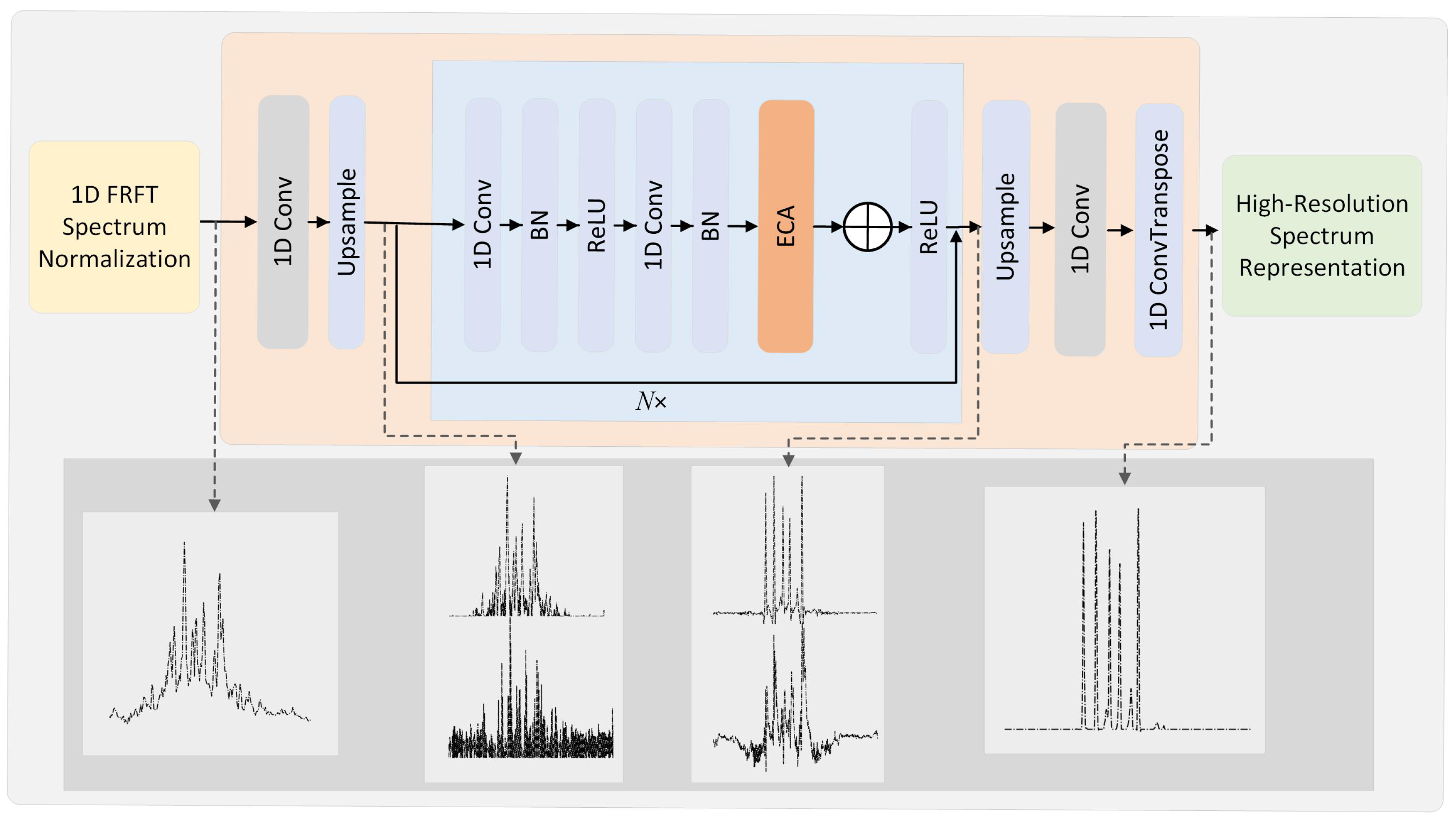
3. Network Structure for High-Resolution Parameter Estimation

This section presents the overall framework of the neural network, which performs high-resolution signal parameter estimation through a deep neural network. As shown in Figure 2, the network framework consists of an input layer, upsampling modules, and high-resolution modules. The specific network design and implementation will be elaborated in detail in the subsequent sections.

3.1. Input Layer

The autocorrelation terms of the signal’s ACCF are first processed using the FrFT to generate the spectrum. One-dimensional slices are then extracted from the spectrum in the $\alpha$-domain. Following this, multiple convolutional kernels are applied to perform convolution operations on the spectrum. This process is fundamentally equivalent to utilizing multiple filters for targeted feature extraction. Specifically, we utilize eight convolutional kernels, each with a kernel size of one × three, to perform feature extraction on the $\alpha$-domain spectrum within different receptive fields and feature patterns. The input to the network can be expressed as follows:

$$X\left(\alpha \right)=X\left(\widehat{\alpha }\right)+w$$

(33)

where $X\left(\widehat{\alpha }\right)$ represents the signal after spectrum superposition and w represents Gaussian white noise. It is particularly noteworthy that before the data are fed into the network for training, normalization of the data is indispensable. This step is critical in the model-training process, as it effectively eliminates dimensional discrepancies in input data across various application scenarios. Without proper normalization, the dimensional effects of the input data could significantly degrade the model’s performance, thereby limiting its applicability across a wider range of scenarios.

3.2. Upsampling Module

The upsampling module is designed to restore low-resolution feature sequences to high-resolution ones, thereby enhancing the accuracy of parameter estimation. This module consists of an upsampling layer and a one-dimensional convolutional module. Considering the computational complexity of FrFT, the sequence length of the input spectrum is typically constrained by the computational burden. The upsampling layer addresses this limitation by further improving the precision of parameter estimation. The convolutional module is responsible for extracting finer spatial information from the high-resolution features, thereby enhancing the model’s ability to represent critical features. This process can be described mathematically as follows:

$$\begin{array}{c}{Y}_{\mathrm{conv}}\left(\alpha \right)=\sum _{k}X(\alpha -k)·W_{\mathrm{conv}}\left(k\right),\\ Y_{\mathrm{up}}\left(\alpha \right)=\sum _k{Y}_{\mathrm{conv}}(f\left(\alpha \right)-m)·W_{\mathrm{up}}\left(m\right).\end{array}$$

(34)

Here, $W_{\mathrm{conv}}$ represents the convolution kernel, $Y_{\mathrm{conv}}$ denotes the output feature map after convolution, f represents the mapping relationship of the upsampling process, $W_{\mathrm{up}}$ corresponds to the weights of the upsampling operation, and $Y_{\mathrm{up}}$ refers to the high-resolution signal obtained after upsampling.

3.3. High-Resolution Module

In the high-resolution module, a one-dimensional convolutional network is utilized to extract features from the upsampled FrFT angle-domain spectrum. To further analyze the characteristics of spectral peaks, residual blocks are stacked to enable deeper feature extraction. The stacking design of residual blocks has been widely proven effective in capturing complex features and significantly enhances the model’s feature extraction capability. As a result, $N=32$ residual blocks are incorporated into the high-resolution module to reinforce the deep-level extraction of time-frequency features. This operation can be formally expressed as follows:

$$Y_{\mathrm{res},i}\left(\alpha \right)=Y_{\mathrm{up}}\left(\alpha \right)+\sum _{i=1}^N\mathrm{Conv}\left(Y_{\mathrm{res},i-1}\left(\alpha \right),W_{\mathrm{res},i}\right)$$

(35)

Considering that traditional one-dimensional composite convolutional modules are limited by their receptive fields, which integrate spatial information only within a fixed range and fail to fully capture interchannel correlations, we introduced a lightweight Efficient Channel Attention (ECA) module into each residual block. The network diagram of the ECA module is shown in Figure 3. It is important to note that “channels” here refer to the multi-channel output features extracted by multiple filters in the input layer. Through local cross-channel interactions via one-dimensional convolution, the ECA module refines coarse features extracted by the convolutional layers, effectively capturing both the spatial correlations of frequency points in the FrFT domain and the dependencies between channels.

The specific computation process of the ECA module is described in the section below. First, global average pooling is applied to the input to compute the mean value across each channel, thereby generating aggregated features. This process can be formally expressed as follows:

$$\begin{array}{c}{Y}_i(\alpha ,c)=\mathrm{Conv}\left(Y_{\mathrm{res},i-1}(\alpha ,c),W_{\mathrm{res},i}\right),\\ z_c={\displaystyle \frac{1}{L}}\sum _{i=1}^L{Y}_i(\alpha ,c),c\in \{1,2,\dots ,C\}.\end{array}$$

(36)

where $z_c$ represents the weight of channel c and L denotes the sequence length. A one-dimensional convolution is then applied to model interaction relationships between channels, generating channel weights. Through the use of a small convolutional kernel k, local relationships between each channel and its neighbors are effectively captured. The specific computation process is expressed as follows:

$${\omega }_c=\sigma \left({\mathrm{Conv}1\mathrm{D}}_k\left(z\right)\right)$$

(37)

Here, ${\mathrm{Conv}1\mathrm{D}}_k$ represents a one-dimensional convolution with a kernel size k and $\sigma$ denotes the activation function. The kernel size k is dynamically adjusted based on the number of channels c. The computation process is defined as follows:

$$k=\psi \left(C\right)={⌈{log}_2\left(C\right)+b⌉}_{\mathrm{odd}}$$

(38)

where $\psi \left(C\right)$ ensures that k is an odd number and b, the bias term, is set to 1. The computational operations conducted after the ECA module has been embedded into the residual block are expressed as follows:

$$Y\prime (\alpha ,c)=Y(\alpha ,c)·{\omega }_c$$

(39)

The output layer of the network consists of a transposed convolutional layer with a kernel size of five, reducing the feature maps from eight channels to a single channel. Then, a sigmoid activation function generates the final frequency representation.

3.4. Optimization Function

The optimization function is a key factor in enhancing network-training performance. The ground-truth coordinates in the FrFT transformation-angle domain are computed using Equation (19) to generate the ground-truth labels for the network. With reference to the approach in [40,41], the optimization function is formulated as a weighted sum of L Gaussian functions, as follows:

$$Tr\left(\alpha \right)=\sum _{l=1}^{L}exp\left(-{\displaystyle \frac{{(\alpha -{\alpha }_l)}^2}{2{\sigma }_{\alpha }^2}}\right)$$

(40)

Here, ${\alpha }_l$ and ${\sigma }_{\alpha }^2$ represent the coordinates of the l-th ground truth and the variance of the corresponding Gaussian function, respectively. ${\sigma }_{\alpha }^2$ denotes the main lobe width of the ground-truth frequency, directly influencing both resolution and detection rate. A smaller ${\sigma }_{\alpha }^2$ improves resolution but, if the value is too small, may inadequately represent the ground-truth frequency, reducing the detection rate. Thus, when designing the loss function, it is crucial to balance resolution and detection rate. The loss function is defined as follows:

$$\mathrm{loss}=\sum {(Y\left(\alpha \right)-Tr\left(\alpha \right))}^2$$

(41)

where $Y\left(\alpha \right)$ represents the network’s output. The network is trained by minimizing the loss function, effectively reducing the gap between the predicted output and the ground truth. Through this process, the network achieves optimized signal processing. We believe that this process enables the network to suppress noise interference and filter out spectral energy associated with suboptimal transformation angles, thus highlighting the main lobe of the optimal transformation angle.

Additionally, the network is capable of correcting spectral peak shifts, aligning the predicted values precisely with the ground truth, and significantly improving spectral resolution. This method not only enhances the network’s capacity to represent target features but also provides more accurate and reliable spectral information for subsequent tasks.

3.5. Computational Complexity

In general, training a neural network requires a significant amount of time due to the iterative weight updates performed by gradient descent. Once training is complete, the input-to-output mapping reduces to a forward pass with comparatively low computational demands. The algorithmic complexity of our neural network’s forward pass is detailed in

Table 1. Time-complexity analysis of computational models across layers.

Model	Layer Number	Time Complexity
1D Convolution Layer	1, 36	$O(L\times K_1\times F)+O(4L\times K_1\times F)$
Upsampling Layer	2, 35	$O(L\times 2\times F^2)+O(2L\times 2\times F^2)$
High Frequency Module	3–34	$O(2L\times K_1\times F^2\times N\times 2)$
1D Convolution Transpose	37	$O(4L\times K_2\times F)$

. The notations in the table are defined as follows: L represents the length of the input sequence; F denotes the number of filters, which is set to eight; $K_1$ and $K_2$ represent the respective kernel sizes of the convolutional layers, set to three and five; and N corresponds to the number of residual blocks, which is set to thirty-two.

4. Simulation Results

In this section, we validate the effectiveness of the proposed method in detecting maneuvering multiple targets with jerk characteristics through numerical simulations. Specifically, we first provide a detailed explanation of the training-parameter settings for the neural-network component. Subsequently, two multi-target scenarios are simulated to conduct a comparative analysis of the proposed method’s performance in different settings. The evaluation focuses on its integration capabilities, detection performance, and parameter-estimation accuracy for multiple maneuvering targets in complex scenarios.

4.1. Network Parameter Setting

During the training process of the neural network, the batch size was set to 64 and the initial learning rate was set to 0.005. The Adam optimizer was employed to minimize the mean squared error (MSE) loss with sum reduction. The network was trained for 200 epochs to ensure convergence. The length of the noisy LFM signals used in the simulation was 256, with the number of signal components randomly set between one and six, enabling the network to handle signals with up to six components. To simplify the training process, the signal amplitude was uniformly set to one, while the noise was modeled as Gaussian white noise with a SNR randomly generated within the range [−10, 20] dB. Considering that primary signal processing is conducted in the transformation-angle domain and that the optimal transformation angle of the FrFT is solely related to the signal’s chirp rate, the normalized chirp rate of the signals was randomly generated within the range [−0.5, 0.5]. For the DFrFT, the transformation-angle range was similarly set to [−0.5, 0.5], with a transformation step size of 0.005. To support network training, a total of 50,000 training samples and 5000 test samples were generated. All samples contained randomly generated noisy signals to ensure data diversity and comprehensive coverage.

4.2. Capacity for the Coherent Integration of Multiple Targets

To evaluate the capacity of the proposed algorithm for integration, we conducted simulation experiments and compared its performance with those of existing methods, with the results demonstrating its superiority. The simulations involved maneuvering targets in varying quantities, with radar parameters set as follows: a carrier frequency of 10 GHz, a sampling frequency of 10 MHz, and a pulse-repetition frequency of 512. We designed two experimental scenarios with varying numbers of targets to test the algorithm’s robustness under different conditions. The motion parameters of the targets are detailed in

Table 2. Target scenarios with corresponding parameters.

Scenario	Target	Distance (km)	Speed (m/s)	Acceleration (m/s2)	Jerk (m/s3)
Scenario 1	Target 1	18.0	200	0	6.0
	Target 2	18.0	200	0	8.0
	Target 3	18.0	200	0	9.5
Scenario 2	Target 1	17.5	−150	0	−7.5
	Target 2	17.8	−150	0	−5.0
	Target 3	17.8	−150	0	−3.0
	Target 4	18.0	−150	0	−1.5
	Target 5	18.1	−150	0	0.5
	Target 6	18.2	−150	0	2.0

. It is worth noting that the parameter settings of the two scenarios were designed such that the targets were indistinguishable in the range, velocity, or acceleration domains, but separable in the jerk domain. This setup can be regarded as an implementation of a resolution method for multiple closely maneuvering targets.

In this experiment, we assigned different SNR values based on the number of targets. Specifically, in Scenario 1 the SNR was 0 dB, while in Scenario 2, the SNR was 15 dB. As shown in Figure 4 and Figure 5, after pulse compression, the target signals exhibit evident RM and DFM effects, which prevent the effective concentration of target energy. As observed in Figure 4b and Figure 5b, through ACCF processing to extract autocorrelation terms, the RM effect is effectively mitigated. To reduce computational complexity, the signal length of the autocorrelation terms processed by ACCF was downsampled to 256, aligning with the input length of the neural network. Furthermore, as shown in Figure 4c and Figure 5c, subsequent FrFT processing addresses the DFM effect, further enhancing energy concentration. However, for detection of multiple targets, the degree of energy concentration remains constrained.

We then compared the integration capabilities of DFrFT [38], FRAC [35], and the proposed method in the transformed angular domain. As observed in Figure 4d–f and Figure 5d–f, where the red line represents the true frequency position of the target, due to the spectral-peak superposition effect, FrFT and FRAC exhibit noticeable peak shifts, resulting in ineffective target focusing and increased risks of false alarms and misjudgments in the number of targets. In contrast, the proposed method demonstrates superior capacity for the detection of multiple targets. It effectively addresses higher-order DFM while avoiding adverse effects caused by spectral peak superposition, thereby providing robust target detection and performance in motion-parameter estimation. Despite the significant improvement in overall estimation performance, it should be noted that in some cases, residual errors may exist, leading to slight frequency shifts.

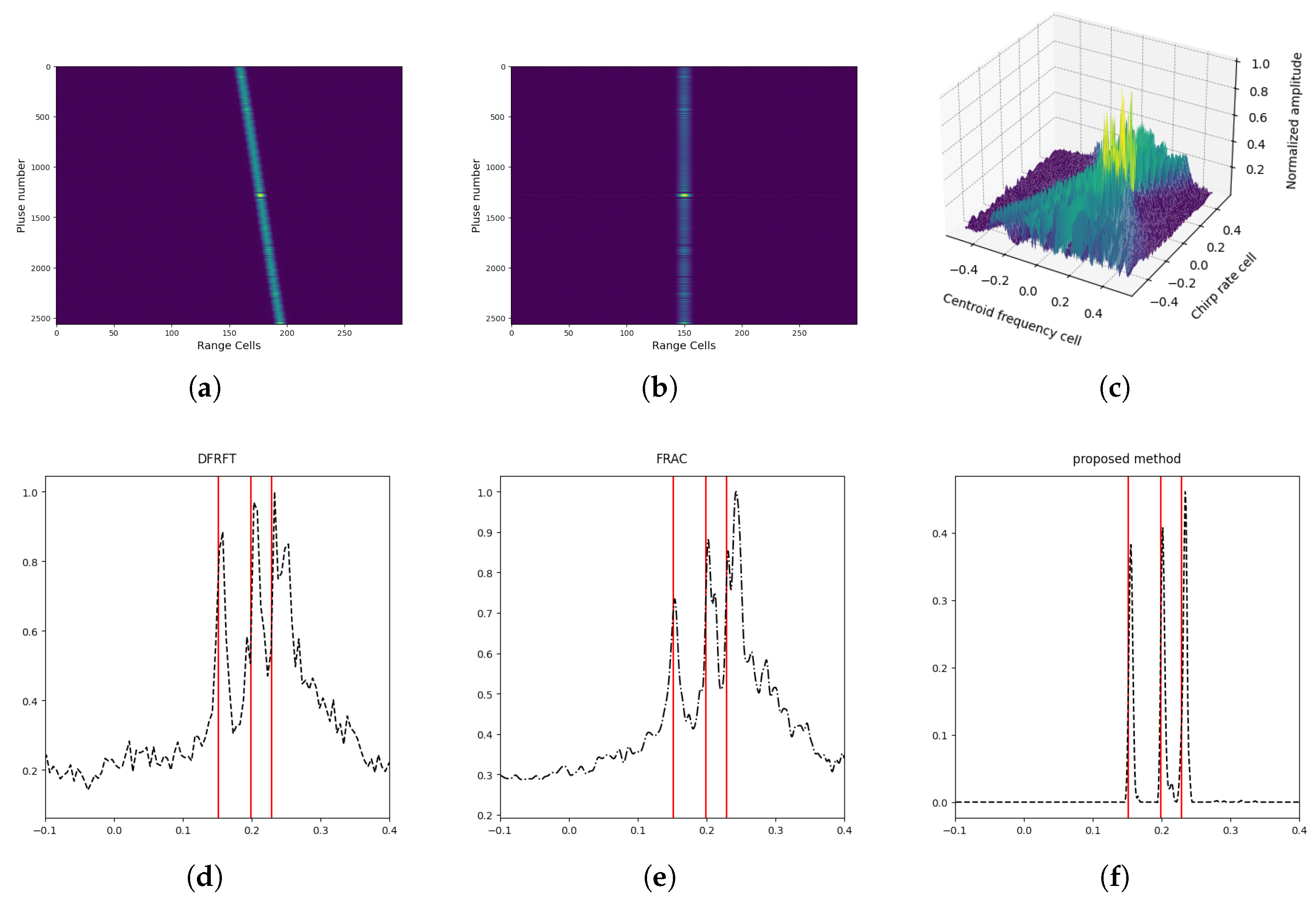
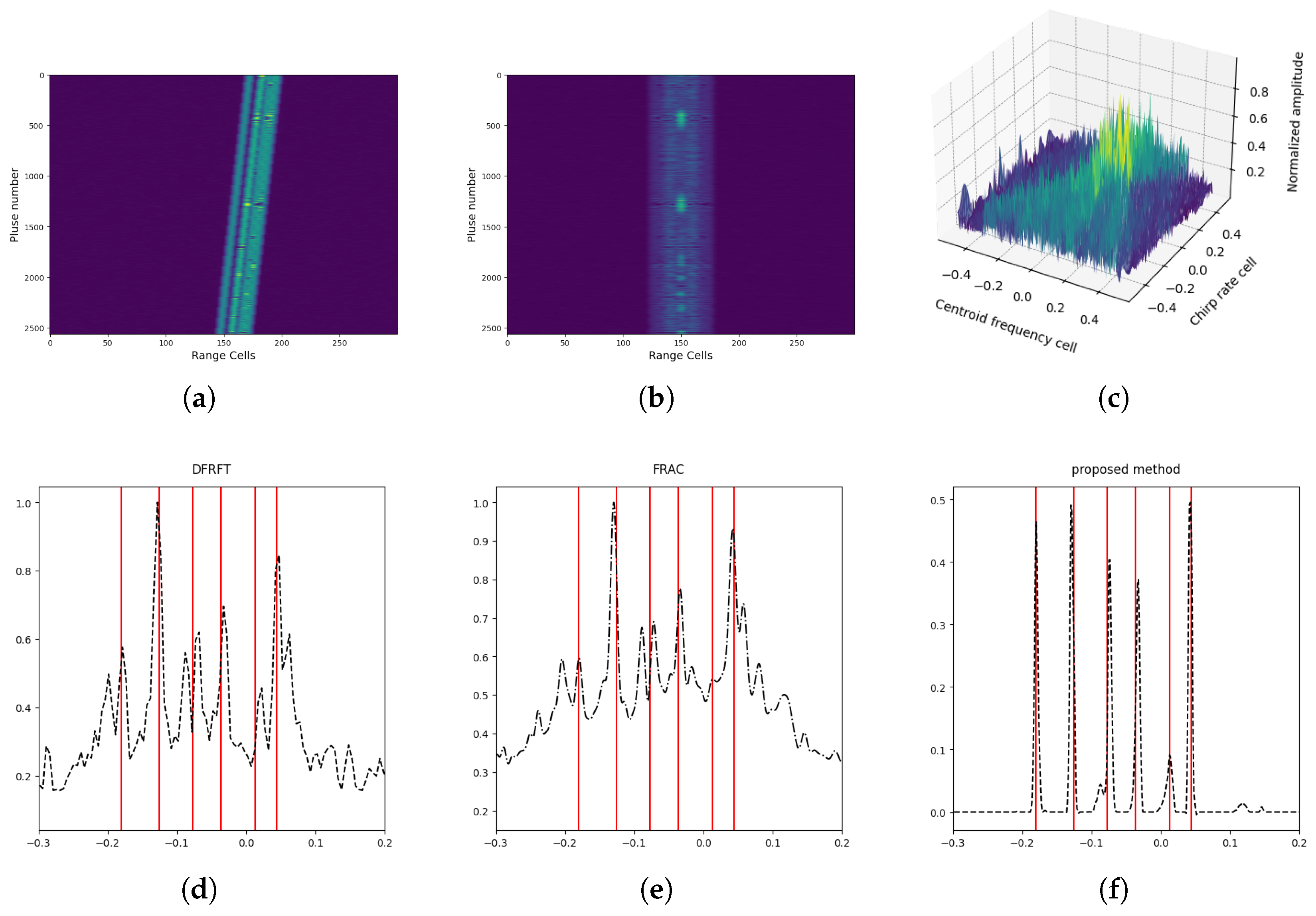
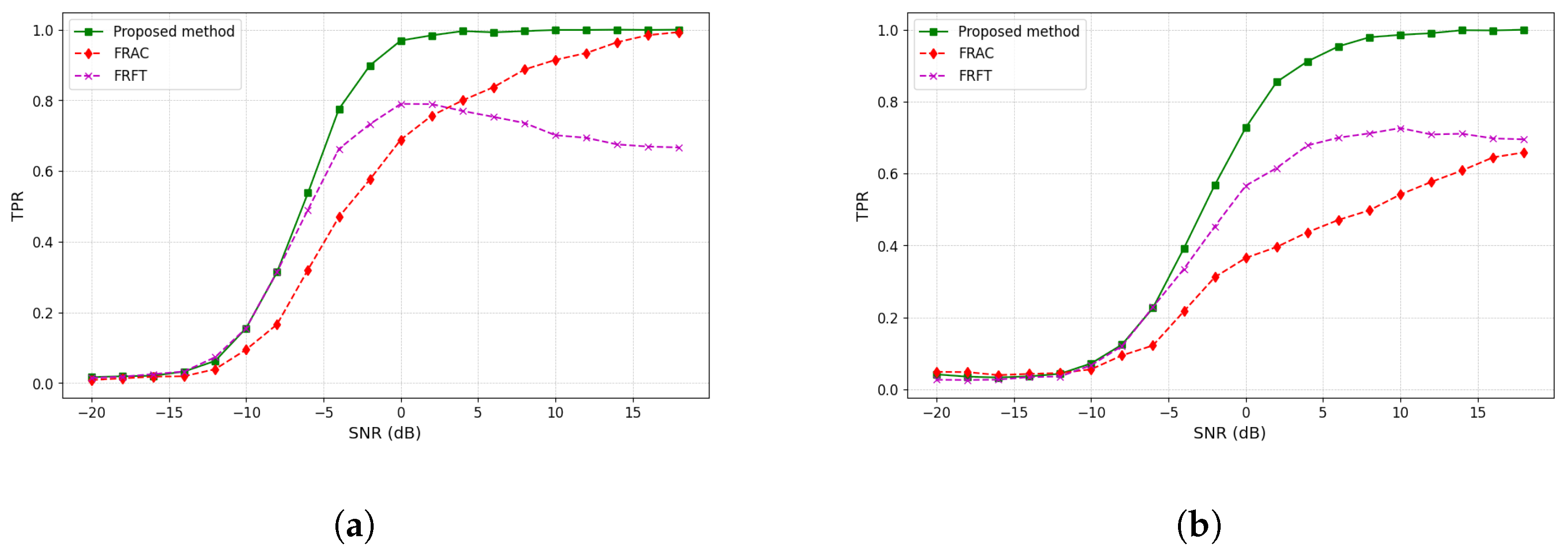
4.3. Capacity for the Detection of Multiple Targets

In this simulation experiment, we used the true positive rate (TPR) to evaluate the detection probability yielded by different algorithms for multiple maneuvering targets. Gaussian white noise was added to the target echoes, with the SNR set in the range of [−20, 20] dB. For each SNR level, 500 Monte Carlo simulations were performed to statistically analyze the detection probability. The target parameters were consistent with those given in Table 2.

The experimental results, as shown in Figure 6, demonstrate that, under varying SNR levels, the proposed algorithm achieves a higher probability of detection of multiple targets compared to FrFT and FRAC. In Scenario 1, the proposed method successfully detects three targets correctly at 0 dB, whereas FRAC achieves full detection accuracy only at 15 dB. On the other hand, FrFT shows a decline in performance as the SNR increases, which we attribute to spectral overlap causing false detections and subsequently affecting the detection rate. In Scenario 2, the proposed method achieves correct detection at 10 dB, while the detection rates of the other two methods ultimately stabilize between 0.6 and 0.7, indicating partial detection of four targets. These results highlight that, in scenarios with varying target counts, the proposed method consistently achieves accurate detection under high-SNR conditions, whereas the use of the other two methods results in a number of missed detections. This further confirms the effectiveness and robustness of the proposed algorithm in detecting multiple maneuvering targets.

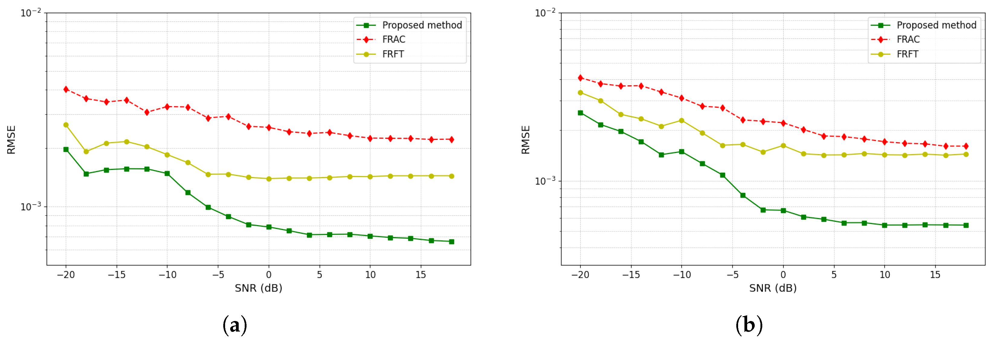
4.4. Parameter Estimation for Multiple Targets

In this experiment, we evaluated the performance of each of multiple methods by calculating the root mean square error (RMSE) for parameter estimation. The target parameters were consistent with those in the previous experiments, with the simulated SNRs in the range [−20, 20] dB. For each SNR level, 500 Monte Carlo simulations were conducted.

The simulation results shown in Figure 7 indicate that the proposed method significantly outperforms other approaches in terms of jerk parameter estimation for multiple targets, achieving a lower RMSE. It is worth noting that, for a fair comparison, we considered only correctly detected targets, as including incorrectly detected targets in the RMSE calculation would lead to significant errors. These findings further indicate that the proposed method performs better in both detection capability and parameter-estimation accuracy, showcasing its strong potential for practical applications.

4.5. Comparison of Computational Efficiency

We compared the computational efficiency of the proposed method with those of other techniques by testing 2000 noisy signals and calculating the average execution time, as shown in

Table 3. Comparison of execution times of different methods.

Methods	Time (ms)
FRFT	47
FRAC	52
Proposed method	66

. Since all three methods perform searches in a one-dimensional space, the computation times for FRFT and FRAC are similar. However, the proposed method, which integrates CNN into the FRFT framework, involves higher computational complexity. Despite this, it demonstrates superior detection performance, particularly when handling multi-component signals.

5. Discussion

The rapid growth of drone technology has introduced significant challenges for traditional radar signal processing methods, particularly in detecting high-maneuverability small targets with low radar cross-sections and complex motion parameters, such as jerk-induced high-order motion. These challenges are exacerbated by issues like RM and DFM, which limit the ability of conventional methods to provide high-precision detection and parameter estimation, especially in low-SNR environments. To address these challenges, the proposed ACCF-FrFT-CNN three-stage processing architecture incorporates the ACCF in the preprocessing stage to eliminate RM and reduce high-order DFM components, setting a solid foundation for subsequent transformations. The FrFT then performs coherent energy integration via optimal rotation angles, improving the multi-target detection capability. Finally, a CNN is employed to mitigate multi-target spectral overlap by learning spectral features, overcoming the core bottlenecks of traditional methods in complex motion scenarios.

Experimental results show that the proposed approach significantly improves spectral energy concentration, multi-target detection rate, and motion parameter estimation accuracy compared to conventional FrFT and FRAC methods. Specifically, target energy in spectral maps is more concentrated, effectively mitigating peak shifts due to spectral overlap. The method demonstrates superior multi-target detection performance in low-SNR environments and achieves lower RMSE in parameter estimation, validating its adaptability to complex maneuvering targets. However, the integration of deep learning modules increases computational complexity. Future research will focus on exploring lightweight network designs and algorithm acceleration strategies to balance performance and real-time requirements, thus facilitating practical engineering applications.

6. Conclusions

To address the challenges of insufficient detection and parameter-estimation accuracy for multiple maneuvering drone targets, this paper proposes a method for the high-resolution detection of multiple targets and parameter estimation that integrates the ACCF, FrFT, and CNN. The method aims to resolve issues caused by RM and DFM due to the higher-order motion parameters of maneuvering targets, overcoming the limitations of traditional methods in achieving coherent integration. Specifically, the proposed method utilizes ACCF to effectively eliminate RM and reduce the impact of higher-order Doppler-frequency modulation. FrFT is then applied to achieve coherent signal integration, while CNN is incorporated to alleviate issues associated with spectral overlap encountered during FrFT processing of multiple targets. This significantly improves detection accuracy and the capacity for parameter estimation. Experimental results demonstrate that the proposed method outperforms existing approaches in terms of detection probability and accuracy of parameter estimation and particularly excels in complex multi-target scenarios, showcasing its strong potential for practical applications.

References

1. Zhu, S.; Liao, G.L.; Yang, D.; Tao, H. A new method for radar high-speed maneuvering weak target detection and imaging. IEEE Geosci. Remote Sens. Lett. 2014, 11, 1175–1179. [Google Scholar] [CrossRef]
2. Hassanien, A.; Vorobyov, S.A.; Gershman, A.B. Moving target parameters estimation in noncoherent MIMO radar systems. IEEE Trans. Signal Process. 2012, 60, 2354–2361. [Google Scholar] [CrossRef]
3. Li, X.; Kong, L.; Cui, G.; Yi, W. A fast detection method for maneuvering target in coherent radar. IEEE Sens. J. 2015, 15, 6722–6729. [Google Scholar] [CrossRef]
4. Bai, X.; Tao, R.; Wang, Z.; Wang, Y. ISAR imaging of a ship target based on parameter estimation of multicomponent quadratic frequency-modulated signals. IEEE Trans. Geosci. Remote Sens. 2014, 52, 1418–1429. [Google Scholar] [CrossRef]
5. Zheng, J.; Su, T.; Zhang, L.; Zhu, W.; Liu, Q.H. ISAR imaging of targets with complex motion based on the chirp rate-quadratic chirp rate distribution. IEEE Trans. Geosci. Remote Sens. 2014, 52, 7276–7289. [Google Scholar] [CrossRef]
6. Zhang, H.; Liu, W.; Zhang, Q.; Liu, B. Joint customer assignment, power allocation, and subchannel allocation in a UAV-based joint radar and communication network. IEEE Internet Things J. 2024, 11, 29643–29660. [Google Scholar] [CrossRef]
7. Geng, L.; Li, Y.; Cheng, W.; Dong, L.; Tan, Y. Joint DOA-range estimation based on bidirectional extension frequency diverse coprime array. In Proceedings of the IGARSS 2023-2023 IEEE International Geoscience and Remote Sensing Symposium, Pasadena, CA, USA, 16–21 July 2023; pp. 4820–4823. [Google Scholar] [CrossRef]
8. Yu, L.; Zhao, Y.; Zhang, Q.; He, F.; Zhang, Y.; Su, Y. Weak and High Maneuvering UAV Detection via Long-Time Coherent Integration Based on KT-BCS-LSM Method. IEEE Trans. Veh. Technol. 2025, 74, 494–509. [Google Scholar] [CrossRef]
9. Wu, W.; Wang, G.H.; Sun, J.P. Polynomial radon-polynomial Fourier transform for near space hypersonic maneuvering target detection. IEEE Trans. Aerosp. Electron. Syst. 2018, 54, 1306–1322. [Google Scholar] [CrossRef]
10. Chen, X.; Huang, Y.; Liu, N.; Guan, J.; He, Y. Radon-fractional ambiguity function-based detection method of low-observable maneuvering target. IEEE Trans. Aerosp. Electron. Syst. 2015, 51, 815–833. [Google Scholar] [CrossRef]
11. Jiang, W.; Liu, H.; Jiu, B.; Zhao, Y.; Li, K.; Zhang, Y. Full-dimensional partial-search generalized Radon–Fourier transform for high-speed maneuvering target detection. IEEE Trans. Aerosp. Electron. Syst. 2024, 60, 5445–5457. [Google Scholar] [CrossRef]
12. Al-Sa’d, M.; Boashash, B.; Gabbouj, M. Design of an optimal piece-wise spline Wigner-Ville distribution for TFD performance evaluation and comparison. IEEE Trans. Signal Process. 2021, 69, 3963–3976. [Google Scholar] [CrossRef]
13. Wang, M.; Chan, A.K.; Chui, C.K. Linear frequency-modulated signal detection using Radon-ambiguity transform. IEEE Trans. Signal Process. 1998, 46, 571–586. [Google Scholar] [CrossRef]
14. Jennison, B.K. Detection of polyphase pulse compression waveforms using the Radon-ambiguity transform. IEEE Trans. Aerosp. Electron. Syst. 2003, 39, 335–343. [Google Scholar] [CrossRef]
15. Xu, J.; Yu, J.; Peng, Y.N.; Xia, X.G. Radon-Fourier transform for radar target detection (II): Blind speed sidelobe suppression. IEEE Trans. Aerosp. Electron. Syst. 2011, 47, 2473–2489. [Google Scholar] [CrossRef]
16. Yu, J.; Xu, J.; Peng, Y.N.; Xia, X.G. Radon-Fourier transform for radar target detection (III): Optimality and fast implementations. IEEE Trans. Aerosp. Electron. Syst. 2012, 48, 991–1004. [Google Scholar] [CrossRef]
17. Niu, Z.; Zheng, J.; Su, T.; Li, W.; Zhang, L. Radar high-speed target detection based on improved minimalized windowed RFT. IEEE J. Sel. Top. Appl. Earth Obs. Remote Sens. 2021, 14, 870–886. [Google Scholar] [CrossRef]
18. Xu, J.; Xia, X.G.; Peng, S.B.; Yu, J.; Peng, Y.N.; Qian, L.C. Radar maneuvering target motion estimation based on generalized Radon-Fourier transform. IEEE Trans. Signal Process. 2012, 60, 6190–6201. [Google Scholar] [CrossRef]
19. Wang, J.; Wu, Y.; Deng, X.; Zhang, L. A GRFT-like method for highly maneuvering target detection via neural network. IEEE Geosci. Remote Sens. Lett. 2024, 21, 1–5. [Google Scholar] [CrossRef]
20. Liu, Q.; Guo, J.; Liang, Z.; Long, T. Motion parameter estimation and HRRP construction for high-speed weak targets based on modified GRFT for synthetic-wideband radar with PRF jittering. IEEE Sens. J. 2021, 21, 23234–23244. [Google Scholar] [CrossRef]
21. Li, X.; Zhao, K.; Wang, M.; Cui, G.; Yeo, T.S. NU-SCGRFT-Based Coherent Integration Method for High-Speed Maneuvering Target Detection and Estimation in Bistatic PRI-Agile Radar. IEEE Trans. Aerosp. Electron. Syst. 2024, 60, 2153–2168. [Google Scholar] [CrossRef]
22. Lv, X.; Bi, G.; Wan, C.; Xing, M. Lv’s distribution: Principle, implementation, properties, and performance. IEEE Trans. Signal Process. 2011, 59, 3576–3591. [Google Scholar] [CrossRef]
23. Kong, L.; Li, X.; Cui, G.; Yi, W.; Yichuan, Y. Coherent integration algorithm for a maneuvering target with high-order range migration. IEEE Trans. Signal Process. 2015, 63, 4474–4486. [Google Scholar] [CrossRef]
24. Zhu, D.; Li, Y.; Zhu, Z. A keystone transform without interpolation for SAR ground moving-target imaging. IEEE Geosci. Remote Sens. Lett. 2007, 4, 18–22. [Google Scholar] [CrossRef]
25. Li, X.; Sun, Z.; Yi, W.; Cui, G.; Kong, L. Fast coherent integration for maneuvering target with high-order range migration via TRT-SKT-LVD. IEEE Trans. Aerosp. Electron. Syst. 2016, 52, 2803–2814. [Google Scholar] [CrossRef]
26. Capus, C.; Brown, K.E. Fractional Fourier transform of the Gaussian and fractional domain signal support. IEE Proc.-Image Signal Process. 2003, 150, 99–106. [Google Scholar] [CrossRef]
27. Capus, C.; Rzhanov, Y.; Linnett, L. The analysis of multiple linear chirp signals. In Proceedings of the IEE Seminar on Time-Scale and Time-Frequency Analysis and Applications, London, UK, 29 February 2000. 4/1–4/7. [Google Scholar] [CrossRef]
28. Serbes, A.; Durak, L. Optimum signal and image recovery by the method of alternating projections in fractional Fourier domains. Commun. Nonlinear Sci. Numer. Simul. 2010, 15, 675–689. [Google Scholar] [CrossRef]
29. Zheng, L.; Shi, D. Maximum amplitude method for estimating compact fractional Fourier domain. IEEE Signal Process. Lett. 2010, 17, 293–296. [Google Scholar] [CrossRef]
30. Serbes, A. On the estimation of LFM signal parameters: Analytical formulation. IEEE Trans. Aerosp. Electron. Syst. 2018, 54, 848–860. [Google Scholar] [CrossRef]
31. Shao, Z.; He, J.; Feng, S. Separation of multicomponent chirp signals using morphological component analysis and fractional Fourier transform. IEEE Geosci. Remote Sens. Lett. 2020, 17, 1343–1347. [Google Scholar] [CrossRef]
32. Aldimashki, O.; Serbes, A. Performance of chirp parameter estimation in the fractional Fourier domains and an algorithm for fast chirp-rate estimation. IEEE Trans. Aerosp. Electron. Syst. 2020, 56, 3685–3700. [Google Scholar] [CrossRef]
33. Yan, B.; Li, Y.; Cheng, W.; Dong, L.; Kou, Q. High-resolution multicomponent LFM parameter estimation based on deep learning. Signal Process. 2025, 227, 109714. [Google Scholar] [CrossRef]
34. Chen, X.; Guan, J.; Liu, N.; He, Y. Maneuvering target detection via Radon-fractional Fourier transform-based long-time coherent integration. IEEE Trans. Signal Process. 2014, 62, 939–953. [Google Scholar] [CrossRef]
35. Moghadasian, S.S. A fast and accurate method for parameter estimation of multi-component LFM signals. IEEE Signal Process. Lett. 2022, 29, 1719–1723. [Google Scholar] [CrossRef]
36. Li, X.; Cui, G.; Kong, L.; Yi, W. Fast non-searching method for maneuvering target detection and motion parameters estimation. IEEE Trans. Signal Process. 2016, 64, 2232–2244. [Google Scholar] [CrossRef]
37. Li, X.; Sun, Z.; Yi, W.; Cui, G.; Kong, L. Detection of maneuvering target with complex motions based on ACCF and FRFT. In Proceedings of the 2017 IEEE Radar Conference (RadarConf), Seattle, WA, USA, 8–12 May 2017; pp. 0017–0020. [Google Scholar] [CrossRef]
38. Ozaktas, H.M.; Arikan, O.; Kutay, M.A.; Bozdagt, G. Digital computation of the fractional Fourier transform. IEEE Trans. Signal Process. 1996, 44, 2141–2150. [Google Scholar] [CrossRef]
39. Xu, H.-F.; Liu, F. Spectrum characteristic analysis of linear frequency-modulated signals in the fractional Fourier domain. J. Signal Process. 2010, 26, 1896–1901. [Google Scholar]
40. Pan, P.; Zhang, Y.; Deng, Z.; Wu, G. Complex-valued frequency estimation network and its applications to superresolution of radar range profiles. IEEE Trans. Geosci. Remote Sens. 2022, 60, 1–12. [Google Scholar] [CrossRef]
41. Pan, P.; Zhang, Y.; Deng, Z.; Qi, W. Deep learning-based 2-D frequency estimation of multiple sinusoidals. IEEE Trans. Neural Netw. Learn. Syst. 2022, 33, 5429–5440. [Google Scholar] [CrossRef]
Figure 1. Diagram of LFM Signal Transformation Using FrFT.
Remotesensing 17 02574 g001
Figure 2. Neural-network architecture for high-resolution parameter estimation.
Remotesensing 17 02574 g002
Figure 3. Diagram of the ECA module.
Remotesensing 17 02574 g003
Figure 4. Coherent integration of multiple maneuvering targets in Scenario 1. (a) Result after pulse compression. (b) Result after ACCF. (c) Integration results of FrFT. (d) 1D p-domain slice of FrFT integration results. (e) Integration results of FRAC. (f) Integration results of the proposed method.
Remotesensing 17 02574 g004
Figure 5. Coherent integration of multiple maneuvering targets in Scenario 2. (a) Result after pulse compression. (b) Result after ACCF. (c) Integration results of FrFT. (d) 1D p-domain slice of FrFT integration results. (e) Integration results of FRAC. (f) Integration results of the proposed method.
Remotesensing 17 02574 g005
Figure 6. Comparison of detection probabilities. (a) Scenario 1. (b) Scenario 2.
Remotesensing 17 02574 g006
Figure 7. Performance in parameter dstimation. (a) Scenario 1. (b) Scenario 2.
Remotesensing 17 02574 g007