Article

Estimation of Leaf, Spike, Stem and Total Biomass of Winter Wheat Under Water-Deficit Conditions Using UAV Multimodal Data and Machine Learning

1
Institute of Environment and Sustainable Development in Agriculture, Chinese Academy of Agricultural Sciences, Beijing 100081, China
2
Dryland Farming Institute, Hebei Academy of Agriculture and Forestry Sciences, Hengshui 053000, China
3
Key Laboratory of Crop Drought Tolerance Research of Hebei Province, Hengshui 053000, China
4
College of Water Resources and Civil Engineering, China Agricultural University, Beijing 100083, China
*
Author to whom correspondence should be addressed.
These authors contributed equally to this work.
Remote Sens. 2025, 17(15), 2562; https://doi.org/10.3390/rs17152562
Submission received: 30 May 2025 / Revised: 15 July 2025 / Accepted: 21 July 2025 / Published: 23 July 2025
(This article belongs to the Section Remote Sensing in Agriculture and Vegetation)

Abstract

Accurate estimation aboveground biomass (AGB) in winter wheat is crucial for yield assessment but remains challenging to achieve non-destructively. Unmanned aerial vehicle (UAV)-based remote sensing offers a promising solution at the plot level. Traditional field sampling methods, such as random plant selection or full-quadrat harvesting, are labor intensive and may introduce substantial errors compared to the canopy-level estimates obtained from UAV imagery. This study proposes a novel method using Fractional Vegetation Coverage (FVC) to adjust field-sampled AGB to per-plant biomass, enhancing the accuracy of AGB estimation using UAV imagery. Correlation analysis and Variance Inflation Factor (VIF) were employed for feature selection, and estimation models for leaf, spike, stem, and total AGB were constructed using Random Forest (RF), Support Vector Machine (SVM), and Neural Network (NN) models. The aim was to evaluate the performance of multimodal data in estimating winter wheat leaves, spikes, stems, and total AGB. Results demonstrated that (1) FVC-adjusted per-plant biomass significantly improved correlations with most indicators, particularly during the filling stage, when the correlation between leaf biomass and NDVI increased by 56.1%; (2) RF and NN models outperformed SVM, with the optimal accuracies being R2 = 0.709, RMSE = 0.114 g for RF, R2 = 0.66, RMSE = 0.08 g for NN, and R2 = 0.557, RMSE = 0.117 g for SVM. Notably, the RF model achieved the highest prediction accuracy for leaf biomass during the flowering stage (R2 = 0.709, RMSE = 0.114); (3) among different water treatments, the R2 values of water and drought treatments were higher 0.723 and 0.742, respectively, indicating strong adaptability. This study provides an economically effective method for monitoring winter wheat growth in the field, contributing to improved agricultural productivity and fertilization management.

1. Introduction

Winter wheat is one of the major food crops in China and plays a pivotal role in grain production and food security. The Huang-Huai-Hai region is the core cultivation area of winter wheat, accounting for over 70% of the national planting area and yield [1]. However, water deficit is the primary limiting factor for winter wheat production in this region [2]. Winter wheat has a high water demand during the growing season, and abnormal weather variations severely affect its growth [3]. The crop aboveground biomass (AGB) is critically important for monitoring crop growth [4], which aids in the formulation of rational irrigation plans, improves water resource use efficiency, and allows timely adjustments in fertilization and pest control measures based on growth conditions, thereby promoting healthy growth and maintaining high yield in winter wheat.
Traditional destructive AGB estimation methods are labor intensive and unsuitable for real-time field monitoring. In recent years, unmanned aerial vehicles (UAVs) have advanced rapidly due to the advantages of flexibility, low cost and wide coverage. By equipping UAVs with sensors such as visible light, multispectral, thermal infrared, hyperspectral, and LiDAR, crop information can be obtained, demonstrating high accuracy in estimating crop phenotypic parameters. For example, UAVs equipped with multispectral and hyperspectral sensors can capture canopy spectral information to estimate leaf chlorophyll content [5], nitrogen content [6], aboveground biomass [7] and yield [8]. Multispectral sensors are widely used in agricultural applications due to their advantages such as high cost-effectiveness and simple operation. In a study on estimating the aboveground biomass (AGB) of winter rapeseed based on UAV multispectral data, Liu et al. [7] used partial least squares regression (PLSR) and Random Forest regression (RF) models for estimation, and the obtained estimation accuracy range was R2 = 0.53–0.71. Among them, the Random Forest model had the highest estimation accuracy, with R2 reaching 0.71 and RMSE being 274.18 kg/ha, while the partial least squares regression model had lower estimation accuracy, with RMSE being 284.09 kg/ha. Hyperspectral and LiDAR sensors have advantages such as hyperspectral resolution [9] and accurate acquisition of target height information [10]. Zhang et al. [9] established an optimal quantitative prediction model of AGB of sugar beet by using hyperspectral data. The best coefficient of determination (R2), root mean square error (RMSE) and residual prediction deviation (RPD) ranged, respectively, from 0.74 to 0.80, 46.17 to 65.68 g/m2 and 1.42 to 1.97 for the rapid growth stage of leaf cluster, 0.78 to 0.80, 30.16 to 37.03 g/m2 and 1.69 to 2.03 for the sugar growth stage, and 0.69 to 0.74, 40.17 to 104.08 g/m2 and 1.61 to 1.95 for the sugar accumulation stage. Zolkos et al. [10] used lidar remote sensing to analyze terrestrial aboveground biomass and found that airborne lidar-derived aboveground biomass models are significantly more accurate than those using radar or passive optical data, while models developed from multisensor metrics are more variable and do not consistently improve biomass estimates. However, these two sensors suffered from high cost and complex operation, which are limited in large-scale applications [11]. Optical sensors mounted on UAV platforms typically capture crop canopy spectral information to form vegetation indices (VIs), which are used to calculate crop growth indicators. In crop phenotyping studies, the information obtained from a single sensor is often inefficient, and estimating crop AGB using only vegetation indices (VIs) can be unstable, especially under conditions of high nitrogen levels and high AGB. VIs tend to lose sensitivity to dense plant canopies, particularly in the later growth stages, when VIs no longer increase with the accumulation of AGB [12]. The combination of UAV sensors has been successfully used to evaluate various crop traits, and the fusion of multimodal data can achieve higher accuracy of phenotypic assessment than any single modality [8,13] since the spectral, texture, thermal and structural information of the canopy are complementary. For example, combining VIs and textural features can reduce the influence of the background and noise, thus mitigating the saturation issue associated with high levels of aboveground biomass [14] and improving the performance of estimation models. Regression methods for analyzing the multimodal data extracted by UAVs include multiple linear regression, partial least squares regression [7], Random Forest [7], and Support Vector Machine (SVM) [15]. Maimaitijiang et al. [8] adopted UAV-based multimodal data fusion, integrating RGB, multispectral and thermal images, and successfully predicted soybean yield. The research results showed that fusing spectral, structural, thermal and texture information obtained by UAVs could significantly improve the prediction accuracy of soybean yield, which was better than that of single-modal data. Specifically, the study compared the prediction results of different sensor combinations and various modeling methods. The result found that multimodal data fusion could provide more comprehensive crop growth information, thereby improving the prediction accuracy of the model. For example, when only a single sensor was used, the spectral information of the multispectral sensor had the highest prediction accuracy, with R2 being 0.515 and RMSE being 20.9%. After fusing RGB, multispectral and thermal infrared information, the prediction accuracy was significantly improved, with R2 reaching 0.72 and RMSE% dropping to 15.9%. In addition, the study also pointed out that multimodal data fusion could enhance the model’s adaptability to spatial changes, reduce the spatial aggregation of prediction errors, and thus improve the stability and robustness of the model. Based on the attention to Multimodal imagery fusion, Ma et al. [13] proposed a novel model termed MultimodalNet for field-scaled yield prediction of winter wheat, which achieved good results at the flowering stage, with a coefficient of determination of 0.741 and a mean absolute percentage error of 6.05%. In recent years, deep learning models have flourished, in the case of large amounts of data, the accuracy of deep learning can be further improved, which becomes possible with advances in hardware, technology, data optimization and collection. However, in actual production scenarios, it is difficult to obtain a large amount of labeled data [16]. Machine learning algorithms have shown advantages in crop phenotyping studies, including efficient training processes and relatively low hardware requirements. Therefore, this article selects machine learning methods such as Random Forest, Support Vector Machine and Neural Network to predict the biomass of winter wheat.
In order to build a biomass estimation model based on UAV data, it is essential to measure biomass by conducting plant sampling. Currently, there are two approaches to plant sampling. One approach involves randomly selecting a certain number of plants within a plot, with the specific number depending on the total number of plants in the plot. Typically, 4–5 plants are sampled [7,17], which may also increase to 20 [18]. The other approach samples all plants within a square meter in the plot [15,19]. In the following step, the measured biomass is matched with the UAV imagery by the position matching method, which uses a handheld GPS to record the spatial range and boundary coordinates of the sampled plants. Then the coordinates are located on the UAV imagery [20,21]. However, when the number of samples is large, this method is undoubtedly time-consuming and labor intensive, limiting its use in previous studies. Similarly, the measured biomass can be matched with UAV imagery by the plot matching method. Some researchers average the AGB of the sampled plants and use the mean value to represent the whole plot [19,22,23]. However, using a small number of the plants to represent the whole plot can result in significant matching errors with the average condition of the community calculated by the UAV imagery. To address this, some researchers [7,24,25] estimate the plot-level AGB by multiplying the dry weight of the sampled plants by the total number of plants in the plot. This method improves the spatial matching accuracy between the sampled plants and the UAV imagery. However, the total number of plants must be obtained through manual counting, which is also time-consuming and labor intensive [26]. Although the plant density is determined before sowing according to the planting area, plant spacing and row spacing [24], the number of plants may change under different water stress conditions at different wheat growth stages, leading to variations in planting density. Given these challenges, there is an urgent need for a rapid and efficient biomass matching method that can improve the representativeness of sampled plants.
When measuring the aboveground biomass, leaves, spikes and stems are separated, dried and weighed separately, which are then summed to obtain the total AGB of the corresponding plant. However, after the jointing stage of winter wheat, the stems are often obscured by the canopy leaves and spikes, making them inaccessible to UAV imagery. Consequently, estimating the total AGB using UAV canopy imagery may be biased. To address this issue, previous studies have introduced plant height (PH) as a robust indicator of the total aboveground biomass [27]. With the development of UAV imaging technology, the difference between the digital surface model (DSM) and the digital elevation model (DEM) is often used to calculate the PH [28]. This DSM–DEM method is limited by bare ground interpolation and image matching errors, and its accuracy is easily affected. Lidar directly generates dense 3D point clouds and penetrates the tree canopy to obtain the true ground elevation [29]. However, the high cost and complex data processing process make it challenging for LiDAR technology in large-scale applications. In addition, since the PH of winter wheat does not increase during flowering stage, it is unclear whether adding PH information can improve the estimation accuracy of the AGB of winter wheat at this time. More studies are still needed to explore the estimation of leaves, spikes, stems, and the total biomass of winter wheat after heading based on UAV images.
Fractional Vegetation Coverage (FVC) represents the ratio of the vertical projection area of the crop canopy to the ground area, serving as an important indicator for characterizing crop growth [30]. Estimating FVC using UAV RGB imagery primarily requires image segmentation, followed by calculating the proportion of crops across the entire field [31], which is used to rectify AGB estimates. To the best of our knowledge, this study was the first to use FVC to rectify the sampled biomass to represent the average individual plant biomass in the plot, and the modified leaves, spikes, stems, and the total AGB were used as estimation objects, respectively. Using UAV RGB, multispectral and thermal images of winter wheat at heading, flowering, and filling stages, the correlation between spectral, texture, temperature, and structural characteristics of winter wheat canopy and the biomass was analyzed, and the accuracy of the Random Forest [32], Support Vector Machine [33] and Neural Network [34] in biomass estimation was explored. The objectives of this study were: (1) to evaluate whether the modified biomass of a single plant could enhance the representativeness of the sampled plants; (2) to compare the performance of the three machine learning models on estimating leaves, spikes, stems and the total AGB of winter wheat., i.e., the Random Forest, Neural Network, and Support Vector Machine.

2. Materials and Methods

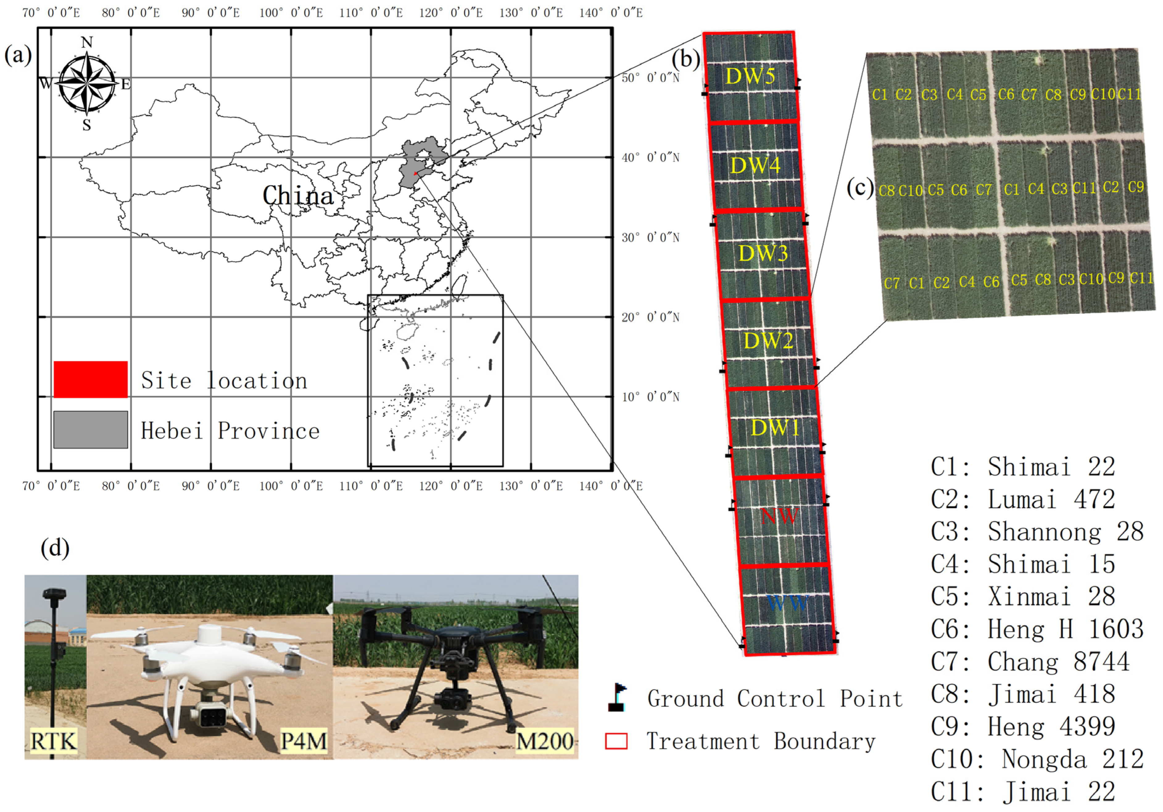
2.1. Experimental Design

The experimental field is located in the experimental station of the Dry Farming Institute of Hebei Academy of Agriculture and Forestry Sciences (37°54′N, 115°42′E). The experimental field is a typical wheat area of Haihe Plain, with an average altitude of 20 m. The annual average precipitation is approximately 497.1 mm, 70% concentrated in July to August, and the annual average temperature is 13.3 °C. The annual effective accumulated temperature (≥10 °C) is 4603.7 °C.
The experiment employed a split-plot design, with each plot covering an area of 9 m2 (1.5 m × 6 m). A total of 231 plots were adopted, including 7 water treatments and 11 wheat cultivars. For each irrigation, the amount of water was 750 m3/ha. The seven treatments included treatment 1 (T1) involving two supplemental irrigations on 3 April 2021 (jointing stage) and 3 May 2021 (flowering stage), treatment 2 involving no supplemental irrigations during the growing season, and treatments 3 to 7 involving one supplemental irrigation at different growth stages, 29 November 2020 (wintering), 10 March 2021 (green-up), 3 April 2021 (jointing), 10 April 2021 (7 days after jointing), and 18 April 2021 (14 days after jointing), respectively. Each treatment was replicated three times (Table 1). Among all treatments, T1 and T2 served as the controls, representing normal growth and complete water stress conditions, respectively. Protective zones were established at the northern and southern ends of the experimental field to minimize the impact of external water sources. Isolation strips, 0.4 m in width, were set between different treatments to reduce mutual influence between water treatments (Figure 1).

2.2. Data Acquisition

This experiment used a DJI Phantom 4 quadcopter (DJI Technology Co., Ltd., Shenzhen, China) equipped with a multispectral imaging system, and a RTK module was used to capture the multispectral images. The multispectral camera integrates five multispectral sensors with central wavelengths at 450 nm, 560 nm, 650 nm, 730 nm, and 840 nm, respectively. Additionally, a DJI M200 quadcopter (DJI Technology Co., Ltd., Shenzhen, China) equipped with a Zenmuse XT2 (DJI Technology Co., Ltd., Shenzhen, China) radiometric dual-lens camera was used to simultaneously capture thermal and RGB images. The thermal imaging sensor is an uncooled thermal infrared camera with a spectral range of 7.5 to 13 µm, and temperature data for each thermal pixel was recorded in degrees Celsius.
The UAV flights were conducted at the key growth stages of the winter wheat, i.e., the heading stage (28 April 2021), the flowering stage (12 May 2021), and the filling stage (21 May 2021). The heading stage refers to the period when the wheat ear begins to emerge from the leaf sheath, which is the starting point for yield formation; the flowering stage is the stage of pollen propagation and pollination, which has a crucial impact on the number of seeds and the potential for grain filling; the filling stage is the peak stage of grain filling and dry matter accumulation. All flights were conducted under clear weather conditions between 10:00 AM and 2:00 PM to capture the UAV images of the wheat canopy. The flying altitude was 50 m, resulting in the spatial resolutions of the multispectral and thermal infrared images of 2.6 cm and 4.6 cm, respectively. The side overlap of all UAV images was 80%, and the forward overlap was 70%. During the flight, a gray target with a reflectance of 50% was placed in the experimental field for radiometric correction of multispectral images. Furthermore, to provide geographic references and improve spatial positioning accuracy for the UAV images, 12 ground control points were established in the experimental field, with geographic coordinates recorded by the handheld GPS.
The field measurement of the AGB was conducted immediately after UAV image acquisition. Five representative plants were selected for destructive sampling in each plot and at each growth stage. The selected samples are uniformly distributed within the plot, with plant height and leaf area index close to the plot’s average levels, avoiding edges and plants affected by pests or diseases, and ensuring that the sample can reflect the overall growth condition of the plot. The plants were washed with clean water to remove surface dust, and the leaves, spikes, and stems were separated. The samples were then oven-dried till a constant mass was achieved. The dry weights of the leaves, spikes, stems, and the entire plant were measured separately.
In summary, a model for estimating the total biomass of wheat leaves, spikes, stems and plants was constructed based on the multimodal characteristics of spectrum, texture, temperature and structure obtained by the UAV remote sensing platform. During the three key growth periods, the correlation between the multimodal data and wheat biomass was analyzed through correlation analysis, and the collinearity between the input indicators was removed through multiple linear regression. Finally, machine learning algorithms such as Random Forest (RF), Support Vector Machine (SVM) and Neural Network (NN) were used to construct regression prediction models for AGB. In order to compare machine learning methods fairly and uniformly, 80% of input features and biomass data were randomly selected as training samples, and the remaining 20% were used as unseen samples to test the performance of the prediction algorithm.

2.3. Image Processing

In this study, the Pix4DMapper software (version 4.5.6, Pix4D SA, Lausanne, Switzerland) was used to process the UAV images of each flight. Radiometric calibration of the multispectral images was performed using the gray reflectance image, and the GCPs were utilized for geometric correction. Subsequently, the RGB, multispectral, and thermal orthomosaic maps were generated. Given the impact of soil and shadows by winter wheat canopies, this study used the method proposed by Wu et al. [35] to remove the pixels of the soil and shadows from the UAV images, obtaining the spectral reflectance of winter wheat canopies.

2.4. Calculation of the Leaf, Spike, Stem, and Total Biomass

Based on the UAV multispectral images, the total number of pixels and the number of winter wheat canopy pixels were calculated for each plot. The FVC was obtained by dividing the canopy pixel count by the total pixel count after radiometric correction, geometric alignment, and vegetation-background separation through threshold segmentation. This method followed the approach proposed by Wu et al. [35], and has been proven to be both reliable and broadly applicable. The theoretical basis for using FVC in biomass correction is consistent with traditional approaches to plot-scale biomass estimation. In previous studies, Liu et al. [7] and Yu et al. [26] calculated aboveground biomass by multiplying the biomass of individual plants by the total number of plants in the plot. In this study, FVC serves as a spatially equivalent scaling factor, effectively replacing manual plant counts. For each plot, five representative winter wheat plants were destructively sampled, and their average dry weights of leaves, spikes, stems, and total biomass were calculated. However, due to the limited number of sampled plants and the spatial heterogeneity in plant density, especially under water-deficit conditions, there may be inconsistencies between the sampled plants and the actual canopy structure of the entire plot. To address this mismatch, FVC was introduced as a correction factor to scale the average individual plant biomass to the plot level, analogous to how plant counts are used in traditional methods. This approach aims to enhance the accuracy and representativeness of biomass estimation by leveraging FVC’s ability to capture spatial variations in canopy coverage that cannot be adequately reflected by plant count alone.
B i o m a s s = M e a s u r e d   d r y   w e i g h t N u m b e r   o f   p l a n t s × F V C
F V C = N u m b e r   o f   p l a n t   p i x e l s N u m b e r   o f   a l l   p i x e l s

2.5. Canopy Feature Extraction and Selection

Although the UAV flights were conducted under clear weather conditions, light changes caused by cloud scattering were inevitable. At the same time, the change in illumination over time might also affect the canopy spectral reflectance. Therefore, it was necessary to standardize the canopy reflectance before extracting the feature extraction [36]. After the image standardization, this study extracted multimodal features for the UAV images, including spectral, texture, thermal, and structure features. Based on previous research findings [13,35], this study adopted 17 VIs that could characterize the aboveground biomass of winter wheat for model construction. The specific names and mathematical expressions of these VIs were provided in Table 2.
The texture is determined by measuring the frequency of grayscale variations or the spatial correlation of colors to establish pixel relationships. Texture features can enhance the accuracy of crop biomass and yield estimation [8]. The gray-level co-occurrence matrix (GLCM) is one of the most widely used texture extraction methods, initially proposed by Haralick in 1973 [50]. This study also adopted GLCM to extract eight texture features in four directions (0°, 45°, 90°, and 135°) for each of the five multispectral bands [8], including Mean, Variance (Var), Homogeneity (Hom), Contrast (Con), Difference (Dis), Entropy (Ent), Second angular moment (Sec) and Correlation (Cor). Furthermore, this study randomly combined the texture features of the five multispectral bands using the simple difference (SD), ratio (SR), and normalization (ND) forms to calculate the texture indices. Next, the texture indices with the highest correlation to the AGB were selected as the canopy texture features. For each of the winter wheat leave, spike, stem, and total plant biomass, the texture indices with the highest correlation to biomass were chosen.
D T I m = T m i T m j
R T I m = T m i T m j
N D T I m = ( T m i T m j ) ( T m i + T m j )
where D T I m , R T I m , and N D T I m represent the difference texture index, the ratio texture index, and the normalized difference texture index of the m-th texture metric. T m i and T m j are the m-th texture metric values of the i-th and j-th multispectral bands, respectively.
The normalized relative canopy temperature (NRCT) [8] and the crop stress index (CSI) [51] are two indicators related to the canopy temperature, which are obtained by UAV thermal infrared images and used to estimate canopy temperature information. NRCT is calculated using canopy temperature, minimum temperature ( T m i n ), and maximum temperature ( T m a x ) throughout the field experiment. CSI is calculated by atmospheric temperature and saturated water vapor pressure difference [35].
N R C T = T c T m i n T c m a x T c m i n
V P D = V P s a t V P a i r
V P s a t = 610.7 × 10 ( 7.5   ×   T c 237.3   +   T c ) 1000
V P a i r = 610.7 × 10 ( 7.5   ×     T   a i r 237.3   + T a i r ) 1000 × R H
where T c is the canopy temperature, T c m a x and T c m i n represent the maximum and minimum values of the canopy temperature in the whole test site, respectively. VPD is the vapor pressure deficit, V P s a t is the saturated vapor pressure of canopy (kPa), and V P a i r is the vapor pressure in the air (kPa). T a i r and RH are the corresponding ambient air temperature (°C) and relative humidity (%), respectively.
In order to obtain accurate PH, the digital elevation model (DEM) of the bare soil in the experimental field was obtained before sowing. During the generation of orthomosaic maps, the digital surface model (DSM) was also obtained. Then, this study calculated the pixel difference between DSM and DEM to obtain the PH. The mean plant height of a plot was used as the PH feature.
In order to gradually optimize the selection of effective regression variables, improve the stability and predictive ability of the model, we used the linear regression in the IBM SPSS Statistics 27 (version 24, IBM Corp., Armonk, NY, USA), the features significantly related to the leaf, spike, stem and total AGB were selected as the input variables of the regression models, and the leaf, spike, stem and total AGB of winter wheat are the target variables. When measuring the severity of multicollinearity between the input variables in a multiple linear regression model, the Variance Inflation Factor (VIF) is widely used, representing the correlation between explanatory variables [52]. Generally speaking, when 0 ≤ VIF < 10, there is no multicollinearity in the regression model. When 10 ≤ VIF ≤ 20, the regression model has a certain multicollinearity. When VIF > 20, the regression model has severe multicollinearity. By gradually eliminating the features with high collinearity, the retained input variables are the features significantly related to the AGB with low collinearity.

2.6. Modeling and Evaluation

This study employed three primary machine learning algorithms: Random Forest (RF), Support Vector Machine (SVM), and Neural Network (NN). Random Forest, based on the decision tree algorithm, estimates by constructing multiple decision trees and synthesizing their results. It offers fast training and is resistant to overfitting [32]. Support Vector Machine, initially designed for classification problems, can also be applied to regression, particularly for high-dimensional data, and is widely used due to its strong generalization ability and robustness to noise [33]. Neural Network, inspired by the behavior of animal neural systems, processes information through interconnected layers of neurons via backpropagation, making it suitable for function estimation or approximation [34]. The performance of the model was evaluated by the coefficient of determination (R2), root mean square error (RMSE) and mean absolute error (MAE). The formula is shown below:
R M S E = 1 n i = 1 n ( y i y i ) 2
M A E = 1 n i = 1 n y i y i
where y i and y i are the measured and estimated values of biomass for sample i, respectively; n is the number of samples. The higher the R2 value, the better the model performance and data fit. The lower the RMSE and MAE values, the higher the estimation accuracy.

3. Results

3.1. Measured Biomass of Winter Wheat

Table 3 showed the statistics of biomass of winter wheat at the heading, flowering and filling stages, including leaf, spike, stem, and total AGB. It could be observed that, especially during the flowering and filling stages, the mean value and coefficient of variation of total AGB were higher, indicating that AGB at these two stages significantly changed. In particular, the coefficient variation of the biomass at the flowering stage reached 32.05%, indicating that the biomass at this stage was significantly different, and the mean AGB at the filling stage was the highest, reaching 22.763 g.

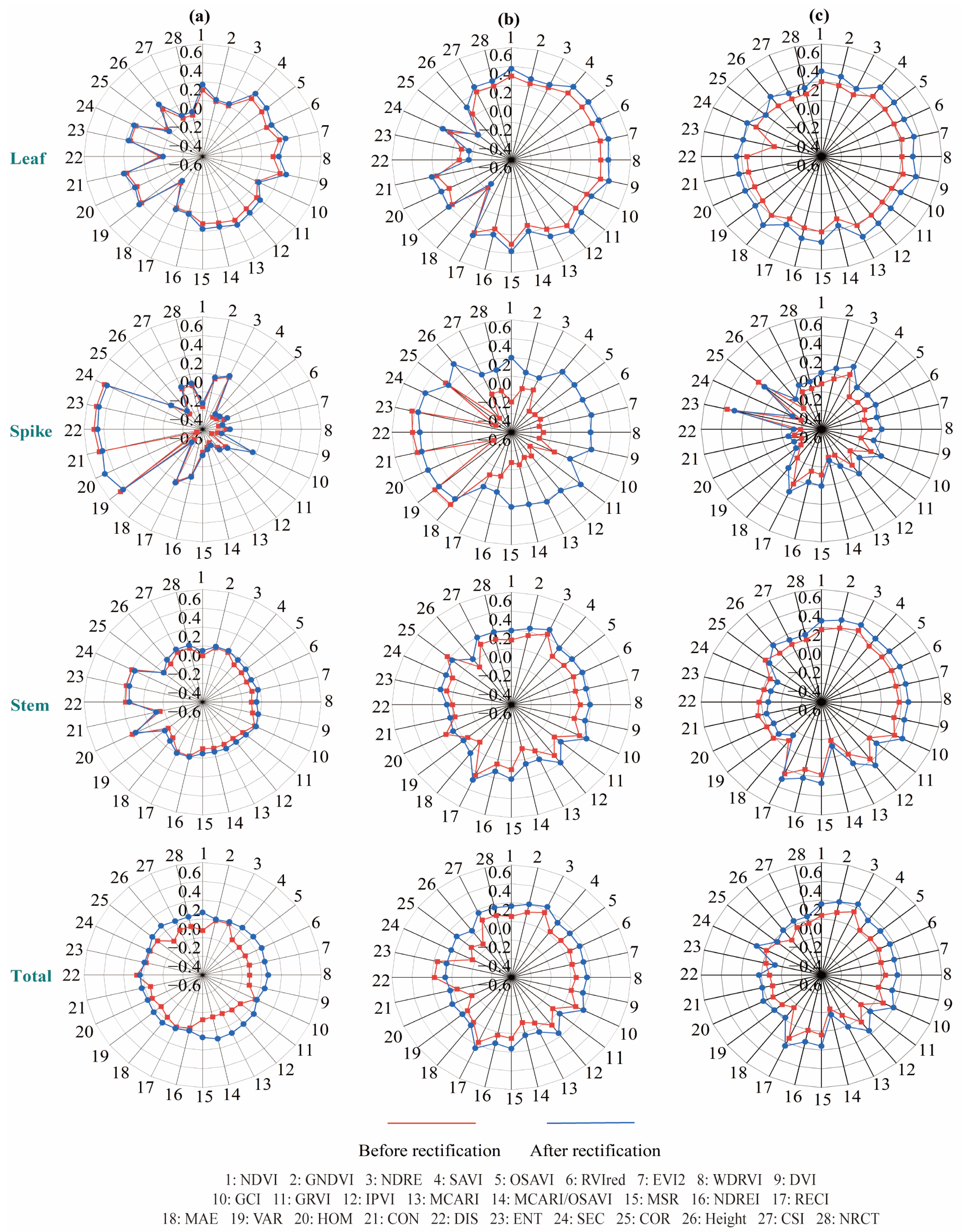
3.2. Correlation Between Biomass Before and After Rectification and Indices

This study extracted 28 features from the UAV multispectral and thermal infrared images, including 17 VIs, eight texture indices, two temperature indices and one structure feature. Correlation analysis was conducted between the features and the leaf, spike, stem, and total AGB, respectively. The results are shown in Figure 2. At the heading stage, the correlation between SAVI, OSAVI, R V I r e d , EVI2, WDRVI, DVI, MCARI, MSR, and the leaf and spike biomass reached a very significant level (p < 0.01), and the correlation coefficient between DVI and the leaf biomass reached 0.268. There was no significant correlation between GNDVI, NDRE, GCI, NDREI, RECI, and the AGB (p > 0.05). At the flowering stage, NDVI, SAVI, OSAVI, R V I r e d , EVI2, WDRVI, IPVI, and MSR were significantly correlated with the leaf, spike, and stem biomass (p < 0.01), and the correlation coefficient between DVI and leaf biomass was 0.406. However, GNDVI, NDRE, GCI, NDREI, and RECI had no significant correlation with the biomass of spike (p > 0.05), GRVI, MCARI, and MCARI/OSAVI were not sensitive to the stem biomass. At the filling stage, NDVI, GNDVI, NDRE, SAVI, OSAVI, R V I r e d , EVI2, WDRVI, DVI, GCI, IPVI, MSR, NDREI, and RECI were significantly correlated with the leaf and the stem biomass (p < 0.01). The correlation coefficient between DVI and the leaf biomass reached 0.365. However, only MCARI/OSAVI reached a very significant level (p < 0.01), NDRE, MCARI and RECI reached a significant level (p < 0.05), and other VIs had no significant correlation (p > 0.05). In summary, with the developmental progress of the winter wheat, the sensitivity of various VIs to the stem biomass showed an overall trend of increasing, and the spike biomass was stable and slightly increased. In contrast, the leaf biomass showed a decreasing trend and the total AGB was stable. Compared with the correlation to the leaf, spike, and stem biomass, the correlation to the total AGB was always low.
All eight texture indices were significantly correlated with the leaf and spike biomass (p < 0.05), some of which were extremely significant (p < 0.01), and the maximum correlation coefficient was 0.497. However, most of the texture indices were not significantly correlated to the stem biomass (p > 0.05), with a few reaching a significant level (p < 0.05). In addition, the texture indices at the three growth stages showed a relatively stable trend. No significant correlation was found between the temperature indices and the total AGB at the heading stage (p > 0.05). However, the biomass of leaf and stem was extremely significant at the flowering stage (p < 0.01) and was significant at the filling stage (p < 0.05). There was a significant correlation between the PH and the spike biomass (p < 0.01), while no significant correlation was found between the leaf, stem, and the total biomass at the heading and the flowering stages (p > 0.05). However, during the filling stage, the correlation between PH and leaves, stems, and the total AGB reached a highly significant level.
In addition, the correlation between the 28 features and the leaf, spike, stem, and total biomass obviously improved after the rectification by using the FVC at the three growth stages (Figure 2), especially the correlation of the leaf biomass, which indicated that multiplying the AGB of a single plant by the FVC as the average level of individual plants in the plot was feasible.

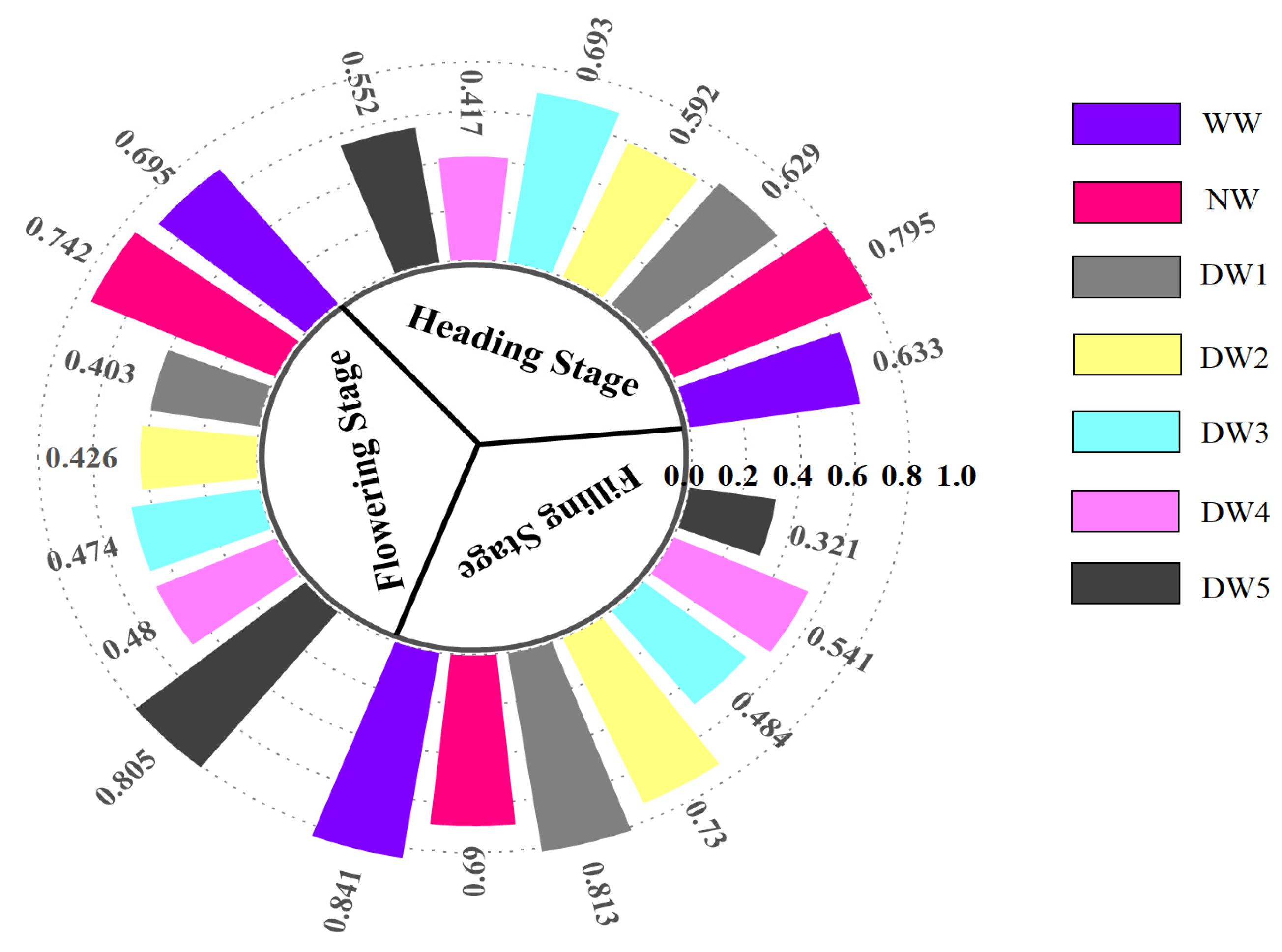
3.3. Evaluation of Leaf, Spike, Stem, and Total Biomass

After the correlation analysis and the collinearity screening by Variance Inflation Factor, the remaining features were the optimal input variables for the estimating models (Table 4). As shown in Table 4, most stages and sectors retained 5 to 7 key features, with commonly retained features including NDVI, GRVI, MCARI/OSAVI, MAE, VAR, and SEM, which reflect biomass variations across different growth stages. Features related to total biomass were primarily retained during the flowering and filling stages, while none were retained at the heading stage. Additionally, leaves retained the highest number of features, followed by spikes and stems. The retained features were mainly composed of vegetation indices and texture metrics, with a lower PH and temperature index.
The results of the AGB using three machine learning models, i.e., RF, SVM, and NN, are shown in Table 5. From the results at the three growth stages, the estimating accuracy of the leaf, spikes, and stem biomass, regardless of the training or the test sets, was much higher than that of the total AGB. Specifically, the accuracy of the leaf biomass estimation was the best at the three stages, followed by the spike and stem biomass. The accuracy of the total AGB was the lowest. The accuracy of the leaf biomass estimation at the flowering stage was the best, the R 2 values of the training and the test sets were 0.653 and 0.709, respectively, the RMSE values were 0.106 g and 0.114 g, respectively, and the MAE values were 0.076 g and 0.091 g, respectively. The best results for the spike, stem and total biomass were also at the flowering stage, with the R2 values of 0.578 and 0.666, respectively, the RMSE values of 0.137 g and 0.154 g, respectively, and the MAE values of 0.107 g and 0.117 g for the spike biomass. The R 2 values for the stem biomass were 0.615 and 0.616, respectively, the RMSE values were 0.336 g and 0.302 g, respectively, and the MAE values were 0.258 g and 0.242 g, respectively. The R 2 , RMSE and MAE of the training and test sets of total AGB were 0.442 and 0.445, respectively, 0.604 g and 0.676 g, respectively, and 0.463 g and 0.516 g, respectively. According to the above results, the estimating accuracy for the total AGB was significantly lower than that for the leaf, spike and stem biomass. In addition, the RF-based and the NN-based models were more accurate than the SVM-based model. As the growth circle progressed, the estimating accuracy decreased, with the highest accuracy at the flowering stage compared with the heading and filling stages.
Figure 3 demonstrated the test results of the optimal model for each growth stage, i.e., NN for the heading stage, RF for the flowering stage and NN for the filling stage. Among the three growth stages, the model constructed by the RF at the flowering stage had the highest accuracy, with an R2 an 0.709, a RMSE value of 0.114 g and a MAE value of 0.091 g. From the heading stage to the filling stage, the R2 first increased and then decreased, reaching its maximum value at the flowering stage.

3.4. Evaluation of Leaf Biomass Under Different Treatments

The results of the optimal model for each growth stage using the seven water treatments are shown in Figure 4. Significant differences among the results of the different water treatments could be observed. The R2 value of WW treatment at the filling stage was the best, which is 0.841, while the R2 value of DW5 at the filling stage was the worst, which was 0.321. In all treatments, the estimated AGB was significantly correlated with the measured AGB. NW had the most significant correlation, and the average R2 of the filling stage reached 0.742, indicating that AGB was the most accurate estimate, followed by WW and DW1, with an R2 of 0.723 and 0.615, respectively.

4. Discussion

4.1. The Rectified Biomass Improved the Representation of the Plot

This study indicated that after converting sampled biomass into rectified individual plant biomass based on the FVC, the correlation between leaf, spike, stem, and total AGB with most multimodal features significantly improved during the heading, flowering, and filling stages. For example, the correlation coefficient between the leaf biomass and EVI2 at the flowering stage increased from 0.314 to 0.4, with an increase of 27.4%. Similarly, the correlation with DVI improved from 0.318 to 0.406, with an increase of 27.7%. At the filling stage, the correlation between the leaf biomass and NDVI increased from 0.198 to 0.309, with an increase of 56.1%, while the correlation with DVI increased from 0.233 to 0.365, with an increase of 56.7%. Considering the potential differences in plant growth under varying drought stress treatments, this study calculated the rectified individual plant biomass using the FVC derived from UAV images and a small number of field-sampled plants, representing the average level of biomass of individual plants in the plot. The results demonstrated that the rectified biomass significantly enhanced the representativeness of the plot biomass. The core mechanism of FVC to improve estimation accuracy may be as follows: first, it strengthens scale matching, bridging the gap between individual plant sampling and remote sensing observations, making sample biomass more consistent with overall canopy characteristics; second, it compensates for spatial heterogeneity. Under water stress, which causes uneven canopy distribution, FVC captures differences between sparse and dense areas, reducing biases from insufficient representativeness of sampling points. Liu et al. and Lu et al. [7,26] argued that relying solely on a small number of sampled plants cannot accurately reflect the growth of the entire plot. Therefore, they incorporated plant density by manually counting the number of plants per unit area in the experimental field, which was then included in the calculation of the AGB. This method aims to account for the overall growth of the plot comprehensively, avoiding significant biomass estimation errors due to a limited number of sampled plants. The AGB was calculated by multiplying the dry weight of each sampled plant by the number of plants in the area. Ultimately, UAV multispectral and RGB images accurately estimated the AGB for winter canola and wheat. Liu et al. [7] combined VIs and texture features for biomass estimation, achieving a RMSE value of 0.27 t/ha, while Lu et al. [26] combined VIs and the PH, which obtained the R2 and RMSE values of 0.78 and 1.34 t/ha, respectively. Although the methods in the two studies mentioned above addressed the challenge of using a small number of sampled plants to represent the entire plot, they still had limitations. Manually counting the number of plants was time-consuming and labor intensive, making it impractical for a large number of experimental plots and large-scale situations. In contrast, the FVC-based method proposed in this study effectively avoided manual plant counting. Moreover, researchers such as Liu et al. [24] and Wang et al. [53] have also focused on improving the representativeness of sampled plants. They proposed a method of calculating AGB based on planting density and sample dry weight, thus achieving precise biomass estimations for potatoes and rice using RGB and hyperspectral images. Liu et al. [24] used the RF model to estimate the potato aboveground biomass, where the R2 and RMSE values were 0.7 and 253.46 kg/ha, respectively. Wang et al. [53] used a quadratic regression model to estimate rice aboveground biomass, achieving an R 2 of 0.777 and an RMSE of 0.223 kg/m2. Both Liu et al. [24] and Wang et al. [53] used the planting density method to account for the varying growth of different plots, reducing the errors from using only a few sampled plants without exhausting labor and time. However, planting density was usually determined before sowing based on the planting area, row spacing, and plant spacing. If a fixed planting density was used throughout the growth circle under different water stress conditions, it might lead to significant errors. The method proposed in this study improved the representativeness of the sampled plants and supported the precise estimation of AGB for winter wheat.

4.2. Comparison of Leaf, Spike, Stem and Total Biomass Results

This study used UAV multimodal images to estimate the leaf, spike, stem, and total biomass of winter wheat. The results showed that the estimating accuracy for each individual organ was significantly higher than for the total AGB, and the estimating accuracy of the leaf biomass was the best. At the flowering stage, the R2 and RMSE of the leaf biomass over the test set were 0.709 and 0.114 g, respectively. For the spike and stem biomass, the R2 values were 0.666 and 0.616, respectively, and the RMSE values were 0.145 g and 0.302 g, respectively, all of which outperformed the total AGB estimations (R2 = 0.445, RMSE = 0.676 g). This finding indicated that the distinct spectral, texture, and structure characteristics exhibited by different organs during winter wheat growth make it more accurate to estimate the biomass of each organ separately. Specifically, the importance of leaves in photosynthesis made them particularly sensitive to spectral signals, especially during the heading, flowering and filling stages when their spectral features were more obvious, resulting in the highest estimation accuracy. The spikes represented nutrient accumulation, while the stems were more related to the structural strength of the plant, to which optical sensors were less sensitive. This aligned with the process in winter wheat, when photosynthetic products gradually shifted to spikes and stems during different growth stages [18]. Specifically, at the flowering and filling stages, the spectral information of the canopy was primarily dominated by leaves and spikes, making the biomass stored in the stems more difficult to be accurately captured. Additionally, direct estimation of the total AGB faced challenges due to the complex nonlinear relationships between the remote sensing features and the biomass. Estimating the total AGB might also introduce redundant information or noise, reducing the estimating accuracy. In contrast, predicting the leaf, spike, and stem biomass separately helped simplify the model, allowing it to better handle the relationships between the biomass and the remote sensing features for each organ, and improving estimating accuracy. There were significant differences in biomass accumulation at various growth stages in winter wheat and separately estimating the biomass of each organ allowed a better understanding of these dynamic changes. Direct estimation of the total AGB might struggle to fully account for these differences. The results of this study agreed with Derraz et al. [54], who estimated the biomass of the rice leaf, spike, and stem biomass using a RF model, achieving R2 values of 0.91, 0.79 and 0.91, respectively, which were all superior to the total AGB (R2 = 0.78). Derraz et al. [54] found that the estimating accuracy for the rice leaf and stem biomass was higher, while the accuracy for the spike biomass was slightly lower, possibly due to the differences in the canopy structure between rice and winter wheat. Moreover, this study focused on biomass estimation at the heading, flowering, and filling stages, while Derraz et al. [54] estimated biomass across the tillering, booting and filling stages as a whole. As one of the most important indicators for estimating AGB, PH should be mainly considered in the application of crop types and growth stages. In this study, the PH of winter wheat will no longer increase during the flowering stage. Thus, including PH information did not improve the accuracy of stem biomass estimation. However, in Zhang et al. [55], the PH played a significant role in AGB estimation at the V6 stage of maize. The estimating accuracy for dry AGB at this stage achieved an R2 of 0.81 and an RMSE of 0.27 t/ha. In conclusion, this study demonstrated that estimating the biomass of the leaf, spike, and stem biomass separately was more effective in capturing the significant differences in the spectral, textural, and structural characteristics of different organs, leading to improved biomass estimation accuracy. Future research will continue to explore the underlying causes of these differences and further enhance the estimating performance by incorporating more remote sensing data and cutting-edge algorithms.

4.3. Comparison of Different Machine Learning Models

To obtain the optimal model for estimating winter wheat AGB, this study employed three machine learning models, i.e., RF, NN, and SVM, which have been widely used in many agricultural research studies. Specifically, the RF model was renowned for its ability to deal with high-dimensional data and its high stability; the NN model could simulate complex nonlinear relationships, and the SVM model exhibited good generalization ability in small sample sizes and high-dimensional spaces. The performance comparison of the models revealed that the RF and NN models generally outperformed the SVM model. The optimal model accuracy R2 and RMSE for the three machine learning methods, RF, SVM, and NN, were 0.709 and 0.114, 0.66 and 0.08, and 0.575 and 0.079, respectively. These results agreed with the study by Wang et al. [56], where the RF model demonstrated higher R 2 and lower RMSE values across various growth stages, indicating that the RF model provided higher accuracy and reliability in winter wheat AGB estimation. RF model utilizes the ensemble method of decision trees to handle high-dimensional features and exhibits stability and accuracy on large datasets, while NN model processes complex data through its nonlinear structure and has high stability and accuracy. Consequently, RF and NN models were suitable for complex agricultural applications such as biomass estimation [57,58]. Although the SVM model has performed well in crop traits estimation studies [59], it still had limitations when facing complex high-dimensional information, making it less effective than the RF and NN models in estimating winter wheat biomass. Furthermore, the dataset in this study covered multiple growth stages, trying to cover more variability in field conditions in the model training and testing. However, the RF and NN models suffered from computational cost at large scales in spite of the superior performance. Future research will explore other cutting-edge models, such as lightweight deep learning models, to further improve the estimating accuracy and reduce the computational costs. In conclusion, the RF and NN models proposed in this study could support the accurate estimation of winter wheat AGB, offering valuable direction and reference for future research and practical applications.
In this study, the contribution of different data sources to the model was not considered. Therefore, future studies will explore how to adaptively determine the feature weights to further improve the estimating accuracy. In addition, this study constructed the estimating models using the AGB data of one growing season of winter wheat. Further analysis using multi-year and multisite data will be conducted to develop a more applicable model to estimate AGB for winter wheat.

5. Conclusions

Based on the FVC extracted from the UAV multimodal images, this study effectively improved the representativeness of field sampling. The UAV-based images of winter wheat at the heading, flowering and filling stages were used to estimate the leaf, spike, stem and total biomass of winter wheat. The results showed that the method of rectifying the AGB by FVC was effective and reliable. Notably, the correlation between leaf biomass and NDVI increased by 56.1% after FVC adjustment during the filling stage, indicating improved spatial consistency between sampled biomass and canopy-level features. Modified biomass significantly improved the representation of individual plants in the plot and supported accurate estimation of the AGB of winter wheat. Among the machine learning models, the RF and NN models outperformed the SVM model, with the RF model achieving the highest estimation accuracy for leaf biomass during the flowering stage (R2 = 0.709, RMSE = 0.114 g). The NN model also performed well (R2 = 0.66), while SVM showed relatively lower performance (R2 = 0.557). The RF and NN models were better than the SVM model in the overall estimating accuracy across the heading, flowering, and filling stages. In addition, the proposed method showed strong adaptability across irrigation conditions, with R2 values reaching 0.742 and 0.723 under drought and well-watered treatments, respectively. As the growth circle progressed, the estimating results at the flowering stage were better than those at the filling and heading stages. Overall, this study provides a robust and non-destructive approach for estimating organ-level and total AGB of winter wheat using UAV-based imagery. The proposed method enhances spatial representation, improves estimation accuracy, and offers valuable potential for high-throughput phenotyping, drought stress assessment, precision field management, and remote sensing-assisted crop breeding. Notably, beyond accurate estimation of total AGB, organ-specific biomass estimation offers unique agronomic insights and application potential. Specifically, leaf biomass, closely associated with photosynthetic activity, serves as a critical indicator for nitrogen diagnosis and guides precision fertilization strategies. Spike biomass, as a key determinant of yield formation, enables early yield forecasting and supports high-yield variety screening. Stem biomass, which is linked to lodging resistance, provides important reference data for stress-resilient breeding and optimization of mechanical harvesting. These findings highlight the broader significance of organ-level biomass estimation in bridging remote sensing technologies with crop physiology and agricultural management.

Author Contributions

Conceptualization, J.L.; methodology, J.L., Y.W. and J.M.; software, J.L. and Y.W.; writing—original draft, J.L.; writing—review and editing, J.L., Y.W. and J.M.; funding acquisition, Y.W., J.M. and B.L.; data curation, B.L., W.Z. and Y.Z.; resources, B.L., W.Z. and Y.Z.; Validation, W.Z. and Y.Z.; Y.W. and J.M. and B.L. contributed equally to this work and should be considered corresponding authors. All authors have read and agreed to the published version of the manuscript.

Funding

This research was funded by the National Natural Science Foundation of China (grant number 32371998), HAAFS Science and Technology Innovation Special Project (grant number 2022KJCXZX-HZS-3), and the Key Research and Development Program of Hebei province (grant number 20326406D).

Data Availability Statement

The data that support the findings of this study are available from the corresponding author upon reasonable request.

Acknowledgments

We would like to express our gratitude to the teachers from the Hebei Academy of Agricultural and Forestry Sciences’ Dryland Water saving Agriculture Experimental Station for their assistance in field data collection.

Conflicts of Interest

The authors declare no conflicts of interest.

References

  1. Zhao, Y.; Han, S.; Zheng, J.; Xue, H.; Li, Z.; Meng, Y.; Li, X.; Yang, X.; Li, Z.; Cai, S.; et al. ChinaWheatYield30m: A 30 m annual winter wheat yield dataset from 2016 to 2021 in China. Earth Syst. Sci. Data 2023, 15, 4047–4063. [Google Scholar] [CrossRef]
  2. Fang, Q.; Zhang, X.; Shao, L.; Chen, S.; Sun, H. Assessing the performance of different irrigation systems on winter wheat under limited water supply. Agric. Water Manag. 2018, 196, 133–143. [Google Scholar] [CrossRef]
  3. Becker, E.; Schmidhalter, U. Evaluation of Yield and Drought Using Active and Passive Spectral Sensing Systems at the Reproductive Stage in Wheat. Front. Plant Sci. 2017, 8, 379. [Google Scholar] [CrossRef] [PubMed]
  4. Han, L.; Yang, G.; Dai, H.; Xu, B.; Yang, H.; Feng, H.; Li, Z.; Yang, X. Modeling maize above-ground biomass based on machine learning approaches using UAV remote-sensing data. Plant Methods 2019, 15, 10. [Google Scholar] [CrossRef] [PubMed]
  5. Uto, K.; Seki, H.; Saito, G.; Kosugi, Y. Characterization of Rice Paddies by a UAV-Mounted Miniature Hyperspectral Sensor System. IEEE J. Sel. Top. Appl. Earth Obs. Remote Sens. 2013, 6, 851–860. [Google Scholar] [CrossRef]
  6. Hu, X.; Caturegli, L.; Corniglia, M.; Gaetani, M.; Grossi, N.; Magni, S.; Migliazzi, M.; Angelini, L.; Mazzoncini, M.; Silvestri, N.; et al. Unmanned Aerial Vehicle to Estimate Nitrogen Status of Turfgrasses. PLoS ONE 2016, 11, e0158268. [Google Scholar] [CrossRef]
  7. Liu, Y.; Liu, S.; Li, J.; Guo, X.; Wang, S.; Lu, J. Estimating biomass of winter oilseed rape using vegetation indices and texture metrics derived from UAV multispectral images. Comput. Electron. Agric. 2019, 166, 105026. [Google Scholar] [CrossRef]
  8. Maimaitijiang, M.; Sagan, V.; Sidike, P.; Hartling, S.; Esposito, F.; Fritschi, F.B. Soybean yield prediction from UAV using multimodal data fusion and deep learning. Remote Sens. Environ. 2020, 237, 111599. [Google Scholar] [CrossRef]
  9. Zhang, J.; Tian, H.; Wang, D.; Li, H.; Mouazen, A.M. A Novel Approach for Estimation of Above-Ground Biomass of Sugar Beet Based on Wavelength Selection and Optimized Support Vector Machine. Remote Sens. 2020, 12, 620. [Google Scholar] [CrossRef]
  10. Zolkos, S.G.; Goetz, S.J.; Dubayah, R. A meta-analysis of terrestrial aboveground biomass estimation using lidar remote sensing. Remote Sens. Environ. 2013, 128, 289–298. [Google Scholar] [CrossRef]
  11. Maimaitijiang, M.; Sagan, V.; Sidike, P.; Maimaitiyiming, M.; Hartling, S.; Peterson, K.T.; Maw, M.J.W.; Shakoor, N.; Mockler, T.; Fritschi, F.B. Vegetation Index Weighted Canopy Volume Model (CVMVI) for soybean biomass estimation from Unmanned Aerial System-based RGB imagery. ISPRS J. Photogramm. Remote Sens. 2019, 151, 27–41. [Google Scholar] [CrossRef]
  12. Liu, Y.; Fan, Y.; Feng, H.; Chen, R.; Bian, M.; Ma, Y.; Yue, J.; Yang, G. Estimating potato above-ground biomass based on vegetation indices and texture features constructed from sensitive bands of UAV hyperspectral imagery. Comput. Electron. Agric. 2024, 220, 108918. [Google Scholar] [CrossRef]
  13. Ma, J.; Liu, B.; Ji, L.; Zhu, Z.; Wu, Y.; Jiao, W. Field-scale yield prediction of winter wheat under different irrigation regimes based on dynamic fusion of multimodal UAV imagery. Int. J. Appl. Earth Obs. Geoinf. 2023, 118, 103293. [Google Scholar] [CrossRef]
  14. Zheng, H.; Cheng, T.; Zhou, M.; Li, D.; Yao, X.; Tian, Y.; Cao, W.; Zhu, Y. Improved estimation of rice aboveground biomass combining textural and spectral analysis of UAV imagery. Precis. Agric. 2018, 20, 611–629. [Google Scholar] [CrossRef]
  15. Atkinson Amorim, J.G.; Schreiber, L.V.; de Souza, M.R.Q.; Negreiros, M.; Susin, A.; Bredemeier, C.; Trentin, C.; Vian, A.L.; de Oliveira Andrades-Filho, C.; Doering, D.; et al. Biomass estimation of spring wheat with machine learning methods using UAV-based multispectral imaging. Int. J. Remote Sens. 2022, 43, 4758–4773. [Google Scholar] [CrossRef]
  16. Yu, D.; Zha, Y.; Sun, Z.; Li, J.; Jin, X.; Zhu, W.; Bian, J.; Ma, L.; Zeng, Y.; Su, Z. Deep convolutional neural networks for estimating maize above-ground biomass using multi-source UAV images: A comparison with traditional machine learning algorithms. Precis. Agric. 2022, 24, 92–113. [Google Scholar] [CrossRef]
  17. Zhu, W.; Sun, Z.; Peng, J.; Huang, Y.; Li, J.; Zhang, J.; Yang, B.; Liao, X. Estimating Maize Above-Ground Biomass Using 3D Point Clouds of Multi-Source Unmanned Aerial Vehicle Data at Multi-Spatial Scales. Remote Sens. 2019, 11, 2678. [Google Scholar] [CrossRef]
  18. Yue, J.; Yang, H.; Yang, G.; Fu, Y.; Wang, H.; Zhou, C. Estimating vertically growing crop above-ground biomass based on UAV remote sensing. Comput. Electron. Agric. 2023, 205, 107627. [Google Scholar] [CrossRef]
  19. Vahidi, M.; Shafian, S.; Thomas, S.; Maguire, R. Pasture Biomass Estimation Using Ultra-High-Resolution RGB UAVs Images and Deep Learning. Remote Sens. 2023, 15, 5714. [Google Scholar] [CrossRef]
  20. Maimaitijiang, M.; Sagan, V.; Sidike, P.; Daloye, A.M.; Erkbol, H.; Fritschi, F.B. Crop Monitoring Using Satellite/UAV Data Fusion and Machine Learning. Remote Sens. 2020, 12, 1357. [Google Scholar] [CrossRef]
  21. De Rosa, D.; Basso, B.; Fasiolo, M.; Friedl, J.; Fulkerson, B.; Grace, P.R.; Rowlings, D.W. Predicting pasture biomass using a statistical model and machine learning algorithm implemented with remotely sensed imagery. Comput. Electron. Agric. 2021, 180, 105880. [Google Scholar] [CrossRef]
  22. Liu, Y.; Feng, H.; Yue, J.; Fan, Y.; Jin, X.; Song, X.; Yang, H.; Yang, G. Estimation of Potato Above-Ground Biomass Based on Vegetation Indices and Green-Edge Parameters Obtained from UAVs. Remote Sens. 2022, 14, 5323. [Google Scholar] [CrossRef]
  23. Wei, L.; Yang, H.; Niu, Y.; Zhang, Y.; Xu, L.; Chai, X. Wheat biomass, yield, and straw-grain ratio estimation from multi-temporal UAV-based RGB and multispectral images. Biosyst. Eng. 2023, 234, 187–205. [Google Scholar] [CrossRef]
  24. Liu, Y.; Feng, H.; Yue, J.; Jin, X.; Fan, Y.; Chen, R.; Bian, M.; Ma, Y.; Song, X.; Yang, G. Improved potato AGB estimates based on UAV RGB and hyperspectral images. Comput. Electron. Agric. 2023, 214, 108260. [Google Scholar] [CrossRef]
  25. Liu, Y.; Feng, H.; Yue, J.; Li, Z.; Yang, G.; Song, X.; Yang, X.; Zhao, Y. Remote-sensing estimation of potato above-ground biomass based on spectral and spatial features extracted from high-definition digital camera images. Comput. Electron. Agric. 2022, 198, 107089. [Google Scholar] [CrossRef]
  26. Lu, N.; Zhou, J.; Han, Z.; Li, D.; Cao, Q.; Yao, X.; Tian, Y.; Zhu, Y.; Cao, W.; Cheng, T. Improved estimation of aboveground biomass in wheat from RGB imagery and point cloud data acquired with a low-cost unmanned aerial vehicle system. Plant Methods 2019, 15, 17. [Google Scholar] [CrossRef] [PubMed]
  27. Næsset, E.; McRoberts, R.E.; Pekkarinen, A.; Saatchi, S.; Santoro, M.; Trier, Ø.D.; Zahabu, E.; Gobakken, T. Use of local and global maps of forest canopy height and aboveground biomass to enhance local estimates of biomass in miombo woodlands in Tanzania. Int. J. Appl. Earth Obs. Geoinf. 2020, 93, 102138. [Google Scholar] [CrossRef]
  28. Yue, J.; Yang, G.; Li, C.; Li, Z.; Wang, Y.; Feng, H.; Xu, B. Estimation of Winter Wheat Above-Ground Biomass Using Unmanned Aerial Vehicle-Based Snapshot Hyperspectral Sensor and Crop Height Improved Models. Remote Sens. 2017, 9, 708. [Google Scholar] [CrossRef]
  29. Li, B.; Xu, X.; Zhang, L.; Han, J.; Bian, C.; Li, G.; Liu, J.; Jin, L. Above-ground biomass estimation and yield prediction in potato by using UAV-based RGB and hyperspectral imaging. ISPRS J. Photogramm. Remote Sens. 2020, 162, 161–172. [Google Scholar] [CrossRef]
  30. Wan, L.; Zhu, J.; Du, X.; Zhang, J.; Han, X.; Zhou, W.; Li, X.; Liu, J.; Liang, F.; He, Y.; et al. A model for phenotyping crop fractional vegetation cover using imagery from unmanned aerial vehicles. J. Exp. Bot. 2021, 72, 4691–4707. [Google Scholar] [CrossRef] [PubMed]
  31. Yan, G.; Li, L.; Coy, A.; Mu, X.; Chen, S.; Xie, D.; Zhang, W.; Shen, Q.; Zhou, H. Improving the estimation of fractional vegetation cover from UAV RGB imagery by colour unmixing. ISPRS J. Photogramm. Remote Sens. 2019, 158, 23–34. [Google Scholar] [CrossRef]
  32. Breiman, L. Random forests. Mach. Learn. 2001, 45, 5–32. [Google Scholar] [CrossRef]
  33. Saunders, C.; Stitson Mo, W.J.; Bottou, L.S.B.; Smola, A. Support Vector Machine—Reference Manual; Department of Computer Science, Royal Holloway, University of London: Amsterdam, The Netherlands, 1998. [Google Scholar]
  34. Ding, S.F.; Jia, W.K.; Su, C.Y.; Zhang, L.W.; Shi, Z.Z. Neural Network Research Progress and Applications in Forecast. In Proceedings of the 5th International Symposium on Neural Networks, Beijing, China, 24–28 September 2008; pp. 783–793. [Google Scholar]
  35. Wu, Y.; Ma, J.; Zhang, W.; Sun, L.; Liu, Y.; Liu, B.; Wang, B.; Chen, Z. Rapid evaluation of drought tolerance of winter wheat cultivars under water-deficit conditions using multi-criteria comprehensive evaluation based on UAV multispectral and thermal images and automatic noise removal. Comput. Electron. Agric. 2024, 218, 108679. [Google Scholar] [CrossRef]
  36. Jiang, J.; Zheng, H.; Ji, X.; Cheng, T.; Tian, Y.; Zhu, Y.; Cao, W.; Ehsani, R.; Yao, X. Analysis and Evaluation of the Image Preprocessing Process of a Six-Band Multispectral Camera Mounted on an Unmanned Aerial Vehicle for Winter Wheat Monitoring. Sensors 2019, 19, 747. [Google Scholar] [CrossRef] [PubMed]
  37. Rouse, J.W.; Haas, R.H.; Schell, J.A.; Deering, D.W. Monitoring Vegetation Systems in the Great Plains with ERTS, Section A. In Proceedings of the NASA Goddard Space Flight Center 3d ERTS-1 Symposyum, Greenbelt, MD, USA, 1 January 1974; Volume 1. [Google Scholar]
  38. Gitelson, A.A.; Gritz, Y.; Merzlyak, M.N. Relationships between leaf chlorophyll content and spectral reflectance and algorithms for non-destructive chlorophyll assessment in higher plant leaves. J. Plant Physiol. 2003, 160, 271–282. [Google Scholar] [CrossRef] [PubMed]
  39. Huete, A.R. A soil-adjusted vegetation index (SAVI). Remote Sens. Environ. 1988, 25, 295–309. [Google Scholar] [CrossRef]
  40. Rondeaux, G.; Steven, M.; Baret, F. Optimization of soil-adjusted vegetation indices. Remote Sens. Environ. 1996, 55, 95–107. [Google Scholar] [CrossRef]
  41. Tucker, C.J. Red and photographic infrared linear combinations for monitoring vegetation. Remote Sens. Environ. 1979, 8, 127–150. [Google Scholar] [CrossRef]
  42. Jiang, Z.; Huete, A.R.; Didan, K.; Miura, T. Development of a two-band enhanced vegetation index without a blue band. Remote Sens. Environ. 2008, 112, 3833–3845. [Google Scholar] [CrossRef]
  43. Gitelson, A.A. Wide dynamic range vegetation index for remote quantification of biophysical characteristics of vegetation. J. Plant Physiol. 2004, 161, 165–173. [Google Scholar] [CrossRef] [PubMed]
  44. Gitelson, A.A.; Viña, A.; Ciganda, V.; Rundquist, D.C.; Arkebauer, T.J. Remote estimation of canopy chlorophyll content in crops. Geophys. Res. Lett. 2005, 32, 8. [Google Scholar] [CrossRef]
  45. Gitelson, A.A.; Merzlyak, M.N. Remote estimation of chlorophyll content in higher plant leaves. Int. J. Remote Sens. 1997, 18, 2691–2697. [Google Scholar] [CrossRef]
  46. Hassan, M.A.; Yang, M.; Rasheed, A.; Jin, X.; Xia, X.; Xiao, Y.; He, Z. Time-Series Multispectral Indices from Unmanned Aerial Vehicle Imagery Reveal Senescence Rate in Bread Wheat. Remote Sens. 2018, 10, 809. [Google Scholar] [CrossRef]
  47. Daughtry, C.S.T.; Walthall, C.L.; Kim, M.S.; de Colstoun, E.B.; McMurtrey, J.E. Estimating corn leaf chlorophyll concentration from leaf and canopy reflectance. Remote Sens. Environ. 2000, 74, 229–239. [Google Scholar] [CrossRef]
  48. Crippen, R.E. Calculating the vegetation index faster. Remote Sens. Environ. 1990, 34, 71–73. [Google Scholar] [CrossRef]
  49. Chen, J.M. Evaluation of Vegetation Indices and a Modified Simple Ratio for Boreal Applications. Can. J. Remote Sens. 2014, 22, 229–242. [Google Scholar] [CrossRef]
  50. Su, H.; Sheng, Y.; Du, P.; Chen, C.; Liu, K. Hyperspectral image classification based on volumetric texture and dimensionality reduction. Front. Earth Sci. 2015, 9, 225–236. [Google Scholar] [CrossRef]
  51. Das, S.; Christopher, J.; Apan, A.; Choudhury, M.R.; Chapman, S.; Menzies, N.W.; Dang, Y.P. Evaluation of water status of wheat genotypes to aid prediction of yield on sodic soils using UAV-thermal imaging and machine learning. Agric. For. Meteorol. 2021, 307, 108477. [Google Scholar] [CrossRef]
  52. Salmeron, R.; Garcia, C.B.; Garcia, J. Variance Inflation Factor and Condition Number in multiple linear regression. J. Stat. Comput. Simul. 2018, 88, 2365–2384. [Google Scholar] [CrossRef]
  53. Wang, Z.; Ma, Y.; Chen, P.; Yang, Y.; Fu, H.; Yang, F.; Raza, M.A.; Guo, C.; Shu, C.; Sun, Y.; et al. Estimation of Rice Aboveground Biomass by Combining Canopy Spectral Reflectance and Unmanned Aerial Vehicle-Based Red Green Blue Imagery Data. Front. Plant Sci. 2022, 13, 903643. [Google Scholar] [CrossRef] [PubMed]
  54. Derraz, R.; Melissa Muharam, F.; Nurulhuda, K.; Ahmad Jaafar, N.; Keng Yap, N. Ensemble and single algorithm models to handle multicollinearity of UAV vegetation indices for predicting rice biomass. Comput. Electron. Agric. 2023, 205, 107621. [Google Scholar] [CrossRef]
  55. Zhang, Y.; Xia, C.; Zhang, X.; Cheng, X.; Feng, G.; Wang, Y.; Gao, Q. Estimating the maize biomass by crop height and narrowband vegetation indices derived from UAV-based hyperspectral images. Ecol. Indic. 2021, 129, 107985. [Google Scholar] [CrossRef]
  56. Wang, L.a.; Zhou, X.; Zhu, X.; Dong, Z.; Guo, W. Estimation of biomass in wheat using random forest regression algorithm and remote sensing data. Crop J. 2016, 4, 212–219. [Google Scholar] [CrossRef]
  57. Fei, S.; Hassan, M.A.; Xiao, Y.; Su, X.; Chen, Z.; Cheng, Q.; Duan, F.; Chen, R.; Ma, Y. UAV-based multi-sensor data fusion and machine learning algorithm for yield prediction in wheat. Precis. Agric. 2022, 24, 187–212. [Google Scholar] [CrossRef] [PubMed]
  58. Aghighi, H.; Azadbakht, M.; Ashourloo, D.; Shahrabi, H.S.; Radiom, S. Machine Learning Regression Techniques for the Silage Maize Yield Prediction Using Time-Series Images of Landsat 8 OLI. IEEE J. Sel. Top. Appl. Earth Obs. Remote Sens. 2018, 11, 4563–4577. [Google Scholar] [CrossRef]
  59. Yuan, H.; Yang, G.; Li, C.; Wang, Y.; Liu, J.; Yu, H.; Feng, H.; Xu, B.; Zhao, X.; Yang, X. Retrieving Soybean Leaf Area Index from Unmanned Aerial Vehicle Hyperspectral Remote Sensing: Analysis of RF, ANN, and SVM Regression Models. Remote Sens. 2017, 9, 309. [Google Scholar] [CrossRef]
Figure 1. Field experimental design included: a location map (a) and an orthomosaic map (b) created from DJI M200 XT2 images, marking the experimental field (red rectangle) and GCPs (black flags). The distribution of the winter wheat cultivar in the deficit-water treatment (c) was identical across the seven treatments. Multispectral images were captured using a Phantom 4-Multispectral UAV, while thermal and RGB images were captured simultaneously using a DJI Matrice 200 with Zenmuse XT2 dual camera (d).
Remotesensing 17 02562 g001
Figure 2. The correlation between biomass and all indices before and after multiplying vegetation coverage ((a) the heading stage, (b) the flowering stage, and (c) the filling stage).
Remotesensing 17 02562 g002
Figure 3. Testing scatter plot of the optimal model at the three stages: (a) the heading stage, (b) the flowering stage, and (c) the filling stage.
Remotesensing 17 02562 g003
Figure 4. Evaluation accuracy of leaf biomass using different treatments in three stages.
Remotesensing 17 02562 g004
Table 1. Different water management schemes for different treatments.
TreatmentSupplemental Irrigation ScheduleGrowth Stage IrrigatedReplicates
T13 April 2021 + 3 May 2021Jointing + flowering3
T2NoneNo irrigation3
T329 November 2020Wintering3
T410 March 2021Green-up3
T53 April 2021Jointing3
T610 April 20217 days after jointing3
T718 April 202114 days after jointing3
Table 2. Vegetation indices (VIs) used in this study.
Vegetation
Index
NameFormulaReferences
NDVINormalized difference vegetation index( R N I R R R )/( R N I R + R R )[37]
GNDVIGreen normalized difference vegetation index( R N I R R G )/( R N I R +   R G )[38]
SAVISoil adjusted vegetation index1.5 × ( R N I R R R )/( R N I R + R R + 0.5)[39]
OSAVIOptimized soil adjusted vegetation index( R N I R R R )/( R N I R R R + 0.16)[40]
R V I r e d Ratio vegetation index R N I R / R R [41]
EVI2Two-band enhanced vegetation index2.5 × ( R N I R R R )/( R N I R + 2.4 × R R + 1)[42]
WDRVIWide dynamic range vegetation index(0.12 × R N I R   R G )/(0.12 × R N I R +   R G )[43]
DVIDifference vegetation index R N I R R R [41]
GCIGreen chlorophyll index R N I R / R G − 1[44]
RECIRed-edge chlorophyll index R N I R / R R E − 1[44]
GRVIGreen–red vegetation index( R G R R )/( R G + R R )[41]
NDRENormalized difference red-edge( R N I R R R E )/( R N I R + R R E )[45]
NDREINormalized difference red-edge index( R R E R G )/( R R E + R G )[46]
MCARIModified chlorophyll absorption in reflectance index(( R R E R R ) − 0.2 × ( R R E R G )) × ( R R E / R R )[47]
MCARI/OSAVI MCARI/OSAVI[47]
IPVIInfrared percentage vegetation index R N I R /( R N I R + R R )[48]
MSRModified simple ratio( R N I R / R R − 1)/( R N I R / R R + 1)[49]
Table 3. Descriptive statistics of measured winter wheat biomass (g).
Acquisition DateSectorNumber of SamplesMinimumMaximumMeanStandard DeviationCoefficient of Variation (%)
Heading StageLeaf2311.9555.4173.4040.71420.97%
Spike0.9215.6842.6040.83331.98%
Stem3.61314.798.6112.09724.35%
Total7.97624.66214.6193.26822.35%
Flowering StageLeaf2311.8246.6993.7260.93625.13%
Spike1.5478.013.7611.20532.05%
Stem5.11521.20910.4912.77326.43%
Total9.16134.5918.0074.52225.11%
Filling StageLeaf2311.7844.9633.1410.63620.26%
Spike4.67517.7410.2242.69226.33%
Stem4.34514.8869.3992.15722.95%
Total11.59935.59422.7634.92321.63%
Table 4. Input variables for the estimating models, (MAE( D T I R , B ) refers to the new texture index obtained by subtracting the reflectance of the red and blue bands generated by MAEN texture, VAR( R T I B , N I R ) refers to the new texture index obtained by the reflectance ratio of the blue and near-infrared bands generated by the Variance texture, and COR( N D T I R E , B ) refers to the new texture index obtained by normalizing the reflectance of the red and blue bands generated by the Correlation texture.
StageSectorIndicators
HeadingLeaf R V I r e d , GRVI, MCARI/OSAVI, MAE( D T I R , B ),
VAR( R T I B , N I R ), CON( R T I B , N I R ), COR( D T I N I R , G ), HOM( R T I N I R , B )
SpikeNDVI, GRVI, MCARI/OSAVI, MAE( D T I N I R , R ),
VAR( R T I N I R , R E ), HOM( D T I N I R , R E ), COR( R T I N I R , B ), Height
StemMAE( R T I R E , B ), VAR( R T I R E , B ), DIS( R T I B , G ), SEM( D T I G , B ), COR( R T I N I R , G )
Total/
FloweringLeafGRVI, NDREI, RECI, MAE( D T I R , B ), VAR( D T I R E , R ),
DIS( D T I N I R , R E ), SEM( R T I N I R , R E ), COR( D T I N I R , R E ), CSI
SpikeNDVI, MCARI/OSAVI, MAE( R T I R , G ), VAR( D T I N I R , G ),
SEM( D T I N I R , R E ), COR( D T I R E , R ), Height, NRCT
StemDVI, GCI, RECI, COR( D T I R E , R ), CSI
TotalDVI, GCI, RECI, CSI
FillingLeafDVI, GRVI, MCARI/OSAVI, VAR( D T I R E , R ),
HOM( R T I R , R E ), ENT( D T I R , G ), COR( N D T I R E , B ), Height, CSI
SpikeMCARI/OSAVI, RECI, CON( R T I G , B ), ENT( D T I N I R , R E ), Height
StemDVI, MCARI/OSAVI, MAE( D T I R , B ), SEM( R T I R E , B ), Height, CSI
TotalIPVI, MCARI/OSAVI, NDREI
Table 5. The accuracy of the RF, SVM and NN models in predicting biomass of leaf, spike and stem. (A slash indicates that no model input parameters are selected).
Flight DateModelsSectorTrain DatasetTest Dataset
R2RMSEMAER2RMSEMAE
April 28RFLeaf0.5520.0970.0730.6050.090.068
Spike0.4930.1060.080.4930.1060.081
Stem0.3810.3070.2260.3270.3770.271
Total//////
SVMLeaf0.4190.1090.080.5750.0790.062
Spike0.560.090.0710.5720.0910.069
Stem0.1160.370.2770.1140.40.302
Total//////
NNLeaf0.550.0940.0720.660.080.055
Spike0.5480.0980.0690.6540.0980.072
Stem0.3030.3330.2690.2760.3390.278
Total//////
May 12RFLeaf0.6530.1060.0760.7090.1140.091
Spike0.5780.1370.1070.6660.1540.117
Stem0.6150.3360.2580.6160.3020.242
Total0.4420.6040.4630.4450.6760.516
SVMLeaf0.5260.1290.1050.5570.1170.099
Spike0.3710.1670.1280.4580.1540.125
Stem0.1490.4520.3430.130.520.39
Total0.1440.7330.5430.0760.8540.681
NNLeaf0.6590.1020.0730.650.1160.072
Spike0.5570.140.1020.5720.1390.109
Stem0.4680.3550.290.5510.4010.328
Total0.210.740.590.1790.6650.54
May 21RFLeaf0.570.0870.0640.5880.0710.066
Spike0.4540.3430.2660.4490.3730.296
Stem0.4360.3040.2330.4730.3320.288
Total0.3310.7420.5910.2580.7250.563
SVMLeaf0.5070.0860.0760.4660.0940.08
Spike0.2450.4030.3020.2370.4410.356
Stem0.3780.3060.2460.4190.3520.282
Total0.0940.8490.6980.1020.8560.707
NNLeaf0.6210.0780.0530.6480.0650.046
Spike0.4580.3480.2690.4580.340.243
Stem0.4540.30.2490.4320.3010.249
Total0.1930.7870.6530.2130.8730.77
Disclaimer/Publisher’s Note: The statements, opinions and data contained in all publications are solely those of the individual author(s) and contributor(s) and not of MDPI and/or the editor(s). MDPI and/or the editor(s) disclaim responsibility for any injury to people or property resulting from any ideas, methods, instructions or products referred to in the content.

