Modeling Multivariable Associations and Inter-Eddy Interactions: A Dual-Graph Learning Framework for Mesoscale Eddy Trajectory Forecasting

Abstract

The precise forecasting of mesoscale eddy trajectories holds significant importance for understanding their mechanisms in driving global oceanic mass and heat transport. However, mesoscale eddies are influenced by numerous stochastic and uncertain factors, leading to substantial fluctuations in their attribute variables. Additionally, the trajectories of eddies are related to historical trends and interact with surrounding eddies. These render the accurate forecasting of mesoscale eddy trajectories a formidable challenge. This study proposes a novel dynamic forecasting framework for eddies’ trajectories, termed EddyGnet, a dual graph neural network framework that synergistically models the complex multivariable association and the spatiotemporal eddy association. In this framework, the dynamic association among eddy attribute variables is first explored by a multivariable association graph (MAG) learning module. Subsequently, the spatial and temporal association among eddies are concurrently analyzed using a spatiotemporal eddy association graph (STEAG) learning module. Finally, a decayed volatility loss function is designed to properly handle the complex and variable data features and improve the forecasting performance. The experimental results on the eddy dataset verify the effectiveness of our proposed EddyGnet, demonstrating superior predictive accuracy and stability compared with existing classical methods. The findings advance the mechanistic understanding of eddy dynamics and provide a transferable paradigm for geoscientific spatiotemporal modeling.

1. Introduction

Mesoscale eddies are integral to the energy cascade within multi-scale oceanic processes [1], facilitating the exchange of heat [2] and carbon dioxide between the ocean and atmosphere, as well as the redistribution of nutrients and resources [3]. These processes are vital for the regulation and transformation of the global climate system [4,5]. Recent research suggests that mesoscale eddies are experiencing unprecedented alterations on a global scale, contributing to accelerated sea-level rise, increased sea surface temperatures [6,7], coastal erosion [8], ocean acidification, and the expansion of deoxygenated “dead zones” [5,9]. Nevertheless, the mechanisms driving these alterations in mesoscale eddy processes and their effects on climate patterns are not yet fully comprehended. Therefore, the accurate forecasting of mesoscale eddy trajectories remains a critical challenge that urgently needs to be addressed in the scientific field.

Mesoscale eddy forecasting has traditionally relied on physical models. For instance, Chelton et al. [10] used the Okubo–Weiss parameterization method to reveal key characteristics such as the westward propagation of mesoscale eddies, emphasizing the nonlinear nature of vortices. Shriver et al. [11] employed a 1/32° Naval Research laboratory Layered Ocean Model (NLOM), demonstrating that increasing model resolution has a greater impact on the depiction of vortices than increasing the number of altimeters. This results in richer and more accurate forecasting information in critical areas such as the Gulf Stream and Kuroshio, as well as at the global ocean average level. Masina and Pinardi [12] developed a quasi-geostrophic numerical model for the initial field in the Adriatic Sea region and conducted a 30-day dynamic forecasting of eddies. They found that changes in topography significantly affect the model’s predictive capabilities. However, these methods are computationally inefficient, and numerous assumptions and simplifications also reduce the accuracy of forecastings.

Data-driven deep learning methods have made significant progress in many fields, including mesoscale eddy forecasting, in recent years. These methods achieve “end-to-end” forecasting, possess strong capabilities for handling nonlinear relationships, and can reveal underlying information to improve forecasting accuracy. For example, in 2019, Ma et al. [13] conducted a 7-day short-term forecasting experiment of eddies in the South China Sea using an improved Convolutional Long Short-Term Memory (Conv-LSTM) network. This method achieved a first-day match rate of 95% for eddies with a diameter greater than 100 km and an average of about 60% over 7 days, effectively validating the feasibility and advantages of deep learning methods in short-term eddy forecasting. In 2020, Wang et al. [14] combined Long Short-Term Memory (LSTM) networks with an improved decision tree algorithm to predict eddy propagation over a 1–4 week period, concluding that eddy attribute forecasting relies more on historical time series, thereby further improving forecasting performance. In 2021, Wang et al. [15] proposed a deep learning framework called MesoGRU. They obtained mesoscale eddy (ME) trajectory and sea level anomaly data from Satellite Oceanographic Data (AVISO) and Copernicus Marine Environment Monitoring Service (CMEMS), processed and analyzed the features to construct a composite dataset, and designed a two-layer GRU network with a new loss function, achieving higher accuracy than single datasets. However, these LSTM- and GRU-based methods still lack long-term memory capabilities. Nian et al. [16] proposed an enhanced Memory-in-Memory (MIM) model with a spatial attention module, which was experimentally validated in the western Pacific region and outperformed methods such as ConvLSTM, significantly promoting ME forecasting and related oceanographic research and observational platform deployment. However, these recurrent networks overly rely on the previous time step. In 2022, Wang et al. [17] constructed a TA-GRU network with a temporal attention layer to predict mesoscale eddies, improving performance by 57%, 44%, and 42% compared with traditional RNN, GRU, and LSTM, respectively, providing a new strategy for accurate mesoscale eddy forecasting. In 2023, Ge et al. [18] argued that relying solely on historical data for mesoscale eddy forecasting is insufficient, leading them to design ETPNet. By enhancing dynamic interaction and representation capabilities with Trace-LSTM, they incorporated ocean current data into the LSTM gate units as a “physical constraint.” When predicting the characteristics of anticyclonic eddies in the North Pacific region from 15°N to 40°N over the next 7 days, their model outperformed other deep learning models. In 2024, Zhang et al. [19] proposed a knowledge fusion neural network method called EddyTPNet, which inputs global eddy movement direction statistics into the decoder as “prior knowledge,” providing insights for solving ocean phenomenon forecasting problems with knowledge fusion neural networks. Tang et al. [20] proposed an ES-ConvGRU network that integrates historical prior statistical information, incorporating interannual variations and seasonal characteristics as prior knowledge into the training process. The 7-day forecasting key indicators were excellent, confirming the advantages of integrating prior information. However, these methods still lack the following important considerations:

Mesoscale eddy processes are influenced by numerous random and uncertain factors. As shown in Figure 1, as mesoscale eddies move, the environmental factors (zonal component (Ugos) and meridian component (Vgos) of absolute geostrophic velocity of the sea surface) change, which in turn cause rapid variations in key variables like the eddy’s radius, displacement, and velocity, and then lead the associations among the variables to become extremely complex. On the other hand, mesoscale eddies exhibit complex driving and response relationships [21]. The motion of one eddy is often influenced by nearby eddies, leading to changes in their trajectories and morphologies. Figure 1 intuitively illustrates the twofold complexity in mesoscale eddy forecasting: the complex multivariable associations and the spatiotemporal interactions among eddies. These complexities present a significant challenge for the accurate forecasting of mesoscale eddy trajectories. They underscore the need to consider both variable associations and inter-eddy interactions in an effective forecasting approach.

To achieve accurate forecasts of mesoscale eddy trajectories, we propose EddyGnet, a framework that integrates graph-based learning for dynamic multivariable and spatiotemporal eddy associations. First, it constructs dynamic association graphs to model the associations between mesoscale eddy variables over time. Second, it incorporates a spatiotemporal learning module using self-attention to capture interactions between eddy trajectories. Finally, a decayed volatility loss function is introduced to handle complex data features and enhance forecasting performance. Experimental results show that EddyGnet outperforms existing time-series forecasting models.

The main contributions of this study can be summarized as follows:

1.

We propose EddyGnet, a framework for mesoscale eddy trajectory forecasting that combines dynamic multivariable and spatiotemporal associations.

2.

We designed a dynamic multivariable association graph (MAG) module that captures associations between mesoscale eddy variables by storing and propagating historical information.

3.

We developed a spatiotemporal eddy association graph (STEAG) module to model the interactions and temporal dependencies of mesoscale eddy trajectories.

2. Data and Methods

2.1. Data

We employ Mean Eddy Trajectory (MET) and Sea Level Anomaly (SLA) data sourced from the Archiving, Validation, and Interpretation of Satellite Oceanographic Data (AVISO) and the Copernicus Marine Environment Monitoring Service (CMEMS). The MET and SLA datasets have a temporal resolution of 1 day. The SLA is a gridded dataset with a spatial resolution of $0.{25}^{\circ }$, while the MET is a time-series data obtained from altimeter satellite data through specific eddy tracking methods.

Specifically, MET data record the evolving locations of eddy centers (longitude and latitude) as they propagate, along with associated dynamic properties such as amplitude, radius, and eddy speed, all derived from SLA-based eddy detection. This eddy-centered trajectory information serves as the primary forecasting target in our model.

In addition to trajectory coordinates, we incorporate auxiliary physical oceanographic variables obtained from CMEMS products, including the following:

• Absolute Dynamic Topography (ADT): the sea surface height above the geoid, reflecting the ocean’s dynamic state;
• Absolute Geostrophic Velocity at the Sea Surface: including both the zonal (Ugos) and meridional (Vgos) components.

These variables are physically linked to eddy dynamics and energy, and are sampled at each trajectory point along the MET to provide oceanographic context during learning. Integrating such variables strengthens the model’s ability to infer latent patterns of eddy propagation by providing insights into the surrounding current structure and flow momentum.

All datasets cover the South China Sea region (0°–25°N, 100°–122°E) from 1 January 1993 to 9 February 2022, spanning nearly 30 years of observations. The long temporal coverage allows the model to learn eddy behavior across seasons, interannual variability, and different oceanographic regimes, improving generalization. The daily granularity further ensures that detailed temporal dynamics are captured.

These satellite-derived datasets are crucial in mesoscale eddy forecasting due to their global coverage, high resolution, and reliable calibration, especially in regions where in situ measurements are sparse or unavailable. By combining trajectory evolution with SLA-derived environmental variables, the model can better capture the complex spatiotemporal interactions influencing eddy movement.

To further integrate these datasets, we filter and match them to extract the properties of the corresponding mesoscale eddy trajectories: longitude, latitude, amplitude, radius, average speed of the eddies’ contours, and average velocity of the eddies’ centers, as well as the marine environmental characteristics of the trajectory points: absolute dynamic topography, zonal component of the absolute geostrophic velocity at the sea surface, and meridional component of the absolute geostrophic velocity at the sea surface.

2.2. Methods

2.2.1. Overall Framework

This section introduces the overall framework of the model, as illustrated in Figure 2. The goal of mesoscale eddy trajectory forecasting is to forecast the future positional coordinates of mesoscale eddies. Given a series of observed historical eddy trajectories’ feature at the time steps $t\in \{1,2,\dots ,T\}$, the spatial coordinates of all eddy trajectories at any given time step are represented as ${\left\{(lo{n}_t^n,la{t}_t^n)\right\}}_{n=1}^N$. Based on the historical trajectories, our objective is to predict the eddy coordinates for future time steps $t\in \{T+1,T+2,\dots ,T+L_{pred}\}$. In our experiments, we set $L_{pred}=7$.

The initial eddy data we input are defined as $X\in {\mathbb{R}}^{N\times T\times F_{in}}$. Here, N denotes the number of eddies. T denotes the length of the observation period. $F_{in}=10$ denotes seven attribute variables of the eddy and three ocean environmental variables: longitude, latitude, amplitude, radius, average speed of eddies’ contour, average velocity of the eddies’ center, angular difference, the absolute dynamic topography, the zonal component of the absolute geostrophic velocity at the sea surface, and the meridian component of the absolute geostrophic velocity at the sea surface.

We independently perform dimensionality expansion on each variable through an embedding module (Section 2.2.2) and then concatenate them, obtaining a new variable dimension $F_e$. Specifically, we extract high-dimensional features from the original data $X\in {\mathbb{R}}^{N\times T\times F_{in}}$ to obtain $Z\in {\mathbb{R}}^{N\times T\times F_e}$.

Next, the MAG learning module captures the evolution characteristics of the associations between variables to obtain improved feature representations, denoted as $Z_C\in {\mathbb{R}}^{N\times T\times F_e}$. Subsequently, the STEAG learning module is employed to model the interactions and motion trends between eddies spatially and temporally through eddy graph learning (EGL) and temporal graph learning (TGL), respectively. It outputs $Z^{STG}$.

Finally, $Z^{STG}$ is used as the initial state input for forecasting. An LSTM model [22] is employed to predict the eddy coordinates for the next seven time steps. The model is optimized using a decayed volatility loss function.

2.2.2. Embedding

Due to the significant fluctuations in the attribute data of eddies, this section employs an unsupervised pretraining of an encoder through time-series representation learning. The encoder is then used to obtain intrinsic features by producing high-dimensional representations of the raw data.

In this section, an encoder based on Dilated Temporal Convolutional Networks (TCNs) is employed. Extensive experiments have demonstrated that TCN exhibits excellent performance and generalization capabilities in time-series data modeling and forecasting tasks, effectively capturing complex temporal patterns and dependencies [23]. Compared with Recurrent Neural Networks (RNNs) and Long Short-Term Memory (LSTM) models, TCN offers higher training efficiency and inference speed. By employing dilated convolutions, TCN significantly expands its receptive field, addressing the issue of insufficient window size in traditional convolutional networks. The formula for TCN is as follows:

$$Z_L^t=\sum _i{X}_L^{(t-r_L·i)}·w_L^i$$

(1)

where $X_L$ represents the input to the L-th layer, $r_L$ is the dilation factor of the L-th layer, and $w_L^i$ denotes the weight matrix of the convolutional kernel at position i in the L-th layer. The final output at time T for the L-th layer is denoted as $Z_L$.

To achieve unsupervised training for the encoder, we employ a triplet contrastive loss. The primary objective is to ensure that, in the embedding space, samples from the same class are closer to each other, while samples from different classes are farther apart. We use the target data as anchor samples and subsequences of the target data as positive samples, and randomly select several data points from other samples as negative samples. These samples are encoded through the TCN and then input into the triplet loss function, which is formulated as follows:

$$TriLoss=max\left(d\right(Z,P)-d(Z,N)+frontier,0)$$

(2)

where Z, P, and N represent the encoded anchor sample, positive sample, and negative sample, respectively. $d(Z,P)$ and $d(Z,N)$ denote the similarity distances between the anchor sample and the positive sample and between the anchor sample and the negative sample, respectively, in the embedding space. $frontier$ is a predefined threshold used to control the difference between positive and negative samples. Ideally, we aim for the similarity distance between the anchor and the negative sample to be at least greater than that between the anchor and the positive sample by a margin determined by the threshold.

After pretraining, we input the historical data at each time step from the original dataset X into the pretrained encoder. We encode each variable independently and then splice them together. The encoder abstracts higher-dimensional features $Z\in {\mathbb{R}}^{N\times T\times F_e}$ from the historical data at each time step.

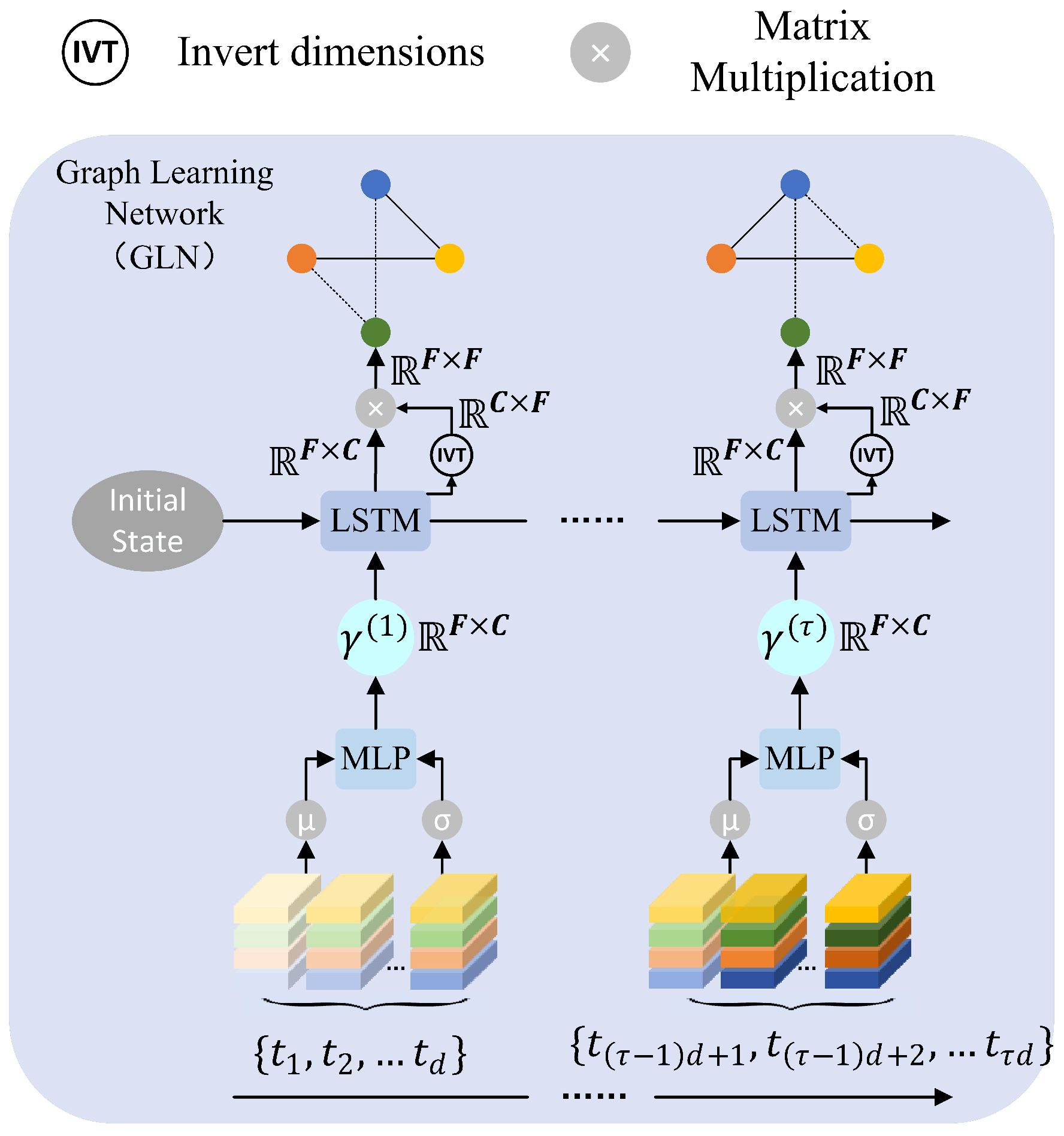
2.2.3. Dynamic Multivariable Association Graph Learning

To intuitively understand the importance of MAG learning in capturing the characteristics of eddy variations, Figure 3 illustrates the changes in displacement, velocity, amplitude, and effective radius during eddy motion, along with the evolution of multivariable association graphs constructed over four time periods based on these variables. In these graphs, the nodes represent individual variables, and the edges depict the correlations between them, with solid lines indicating positive correlations and dashed lines representing negative correlations. As shown in the figure, the structure of the eddy multivariable association graph undergoes significant changes over time.

The MAG learning module is designed to learn the graph structure for each time period, thereby effectively characterizing the evolution of the graph structure over time. Specifically, the adjacency matrix $A=\left\{a_{(m,n)}\right|m,n=1,\dots ,F_e\}$ is defined to represent the associations between each pair of variables.

It is important to note that, during the process of learning the multivariable association graph structure, the channels of different variables should remain independent to avoid interference caused by the premature fusion of variables. To achieve this, we expand the data shape to $Z\in {\mathbb{R}}^{N\times T\times F_e\times C}$, where C represents the augmented dimension for each variable. Z is then fed into the multivariable association graph learning module. The corresponding formula is as follows:

$$\begin{array}{cc}\hfill A_{tseg}^{\tau }& ={\Gamma }_a(Z_{tseg}^{\tau },state)\hfill \end{array}$$

(3)

$$\begin{array}{cc}\hfill Z_{(tseq,\tau )}^{out}& ={\Gamma }_g(A_{tseg}^{\tau },Z_{tseg}^{\tau })\hfill \end{array}$$

(4)

$$\begin{array}{cc}\hfill Z^{out}& =\mathrm{concat}\{Z_{(tseg,1)}^{out},Z_{(tseg,2)}^{out},\dots \}\hfill \end{array}$$

(5)

where $Z_{tseg}^{\tau }$ represents the input of the network for the $\tau$-th time segment, where each time segment has a length of d, and the $\tau \in [1,T/d]$ state represents the dynamically updated state, while ${\Gamma }_a$ denotes the Graph Learning Network (GLN), and $A_{tseg}^{\tau }$ is the graph structure obtained for the $\tau$-th time segment, with the vertex set representing the variable features $F_e$ and the edge set representing the similarity distance between variables ${\left(a_{(m,n)}\right)}_{F_e\times F_e}$. ${\Gamma }_g$ represents the graph convolution operation, and $Z_{(tseg,\tau )}^{out}$ is the output of the graph convolution for the $\tau$-th time segment. Finally, $Z^{out}\in {\mathbb{R}}^{N\times T\times F_e\times C}$ is the final output obtained by concatenating the results from multiple time segments.

The Graph Learning Network (GLN) aims to learn dynamic multivariable correlations based on graphs, with its model structure illustrated in Figure 4. Z is divided into multiple data segments of equal time intervals d, denoted as $Z_{tseg}\in {\mathbb{R}}^{d\times N\times F_e\times C}$. To assess the similarity of different variables within a single time interval, the mean and variance serve as effective indicators. We compute the mean and variance of the data over d time steps and fuse them using an MLP (Multi-Layer Perceptron). The detailed process is as follows:

$${\gamma }_{tseg}^{\tau }=\mathrm{MLP}\left(\mathrm{concat}(\mu \left(Z_{tseg}^{\tau }\right),\sigma \left(Z_{tseg}^{\tau }\right))\right)$$

(6)

where $\mu$ represents the calculation of the mean, $\sigma$ represents the calculation of the variance, and concat refers to the concatenation of channel layers. The MLP is then applied to produce the output ${\gamma }_{tseg}^{\tau }\in {\mathbb{R}}^{N\times F_e\times C}$.

The multivariable associations learned within each time segment are passed along sequentially using an LSTM. The LSTM, a simple yet powerful variant of recurrent neural networks, is employed in this study to model the temporal propagation of the graph. The sequence $[{\gamma }_{tseg}^1,{\gamma }_{tseg}^2,\dots {\gamma }_{tseg}^{\tau }\dots {\gamma }_{tseg}^{T/d}]$ is fed into the LSTM, producing $Y_{tseg}^{\tau }$ as the output for the $\tau$-th time segment.

Next, $Y_{tseg}^{\tau }\in {\mathbb{R}}^{N\times F_e\times C}$ is multiplied by its transpose to obtain the matrix $A_{tseg}^{\tau }\in {\mathbb{R}}^{N\times F_e\times F_e}$. The values of this matrix reflect the similarities between variables, which are used as the edge weights of the graph structure.

The graph convolution operation integrates the C-dimensional feature of the original data $Z_{tseg}^{\tau }\in {\mathbb{R}}^{d\times N\times F_e\times C}$ using the graph structure matrix $A_{tseg}^{\tau }\in {\mathbb{R}}^{N\times F_e\times F_e}$, resulting in the eddy feature $Z^d\in {\mathbb{R}}^{d\times N\times F_e\times C}$. The outputs from all time segments are concatenated, yielding $Z^{out}\in {\mathbb{R}}^{N\times T\times F_e\times C}$.

To reduce model complexity and facilitate learning in subsequent modules, the F-dimensional and C-dimensional channels are flattened. Then, a linear layer is applied to reduce the dimensionality to $F_e$, resulting in $Z^C\in {\mathbb{R}}^{N\times T\times F_e}$. The process is as follows:

$$Z^C=\mathrm{Linear}(Z^{out}.\mathrm{view}(N,T,-1),W_C)$$

(7)

where $\mathrm{view}(N,T,-1)$ denotes the merging of the remaining dimensions, transforming $Z^{out}$ into $N\times T\times (F_e\times C)$, $W_C\in {\mathbb{R}}^{((F\times C)\times F_e)}$.

2.2.4. Spatiotemporal Eddy Association Graph Learning

Mesoscale eddies usually do not exist in isolation. For example, there are dipole eddies in which warm and cold eddies appear in pairs, as well as gear-like eddies [21]. During the processes of eddies coupling and decoupling, the motion trajectories of the eddies will be altered. The past motion state of an eddy also has a direct influence on its future motion. Observations made between eddies and across adjacent time steps are not independent but are dynamically interrelated. This STEAG learning module focuses on jointly learning temporal dependencies (i.e., the correlation between the eddy’s states at different times) and eddy-to-eddy interactions to enable effective spatiotemporal forecastings.

Using $Z^C\in {\mathbb{R}}^{N\times T\times F_e}$ as input, two graph structures are learned to represent temporal dependencies of each eddy and eddy–eddy interaction, as shown in Figure 5. The TGL branch generates a temporal weighted graph $G_T=\left\{G_{(T,n)}\right|n=1,\dots ,N\}\in {\mathbb{R}}^{N\times T\times T}$, which encodes the association scores across T time steps. Simultaneously, the EGL branch constructs an eddy weighted graph $G_E=\left\{G_{(E,t)}\right|t=1,\dots ,T\}\in {\mathbb{R}}^{T\times N\times N}$, representing the interaction scores among N eddies.

Finally, $G_T$ and $G_E$ are integrated into the eddy features to output the spatiotemporal eddy association features $Z^{STG}$.

Temporal Dependency Learning

The primary task in generating a temporal graph is to obtain the node features $V_n=\left\{v_n^t\right|t=1,\dots ,T\}$, which represent the features of the n-th node at all time steps. Graph convolution operates on the nodes at all time points in parallel, which will cause the loss of the temporal information of the nodes. To incorporate temporal information, positional encoding is embedded into the input $Z^C$. The design of the positional encoding follows the classical Transformer architecture, as follows:

$$\begin{array}{cc}\hfill P{E}_{(t,2a)}& =sin\left({\displaystyle \frac{t}{10,{000}^{\frac{2a}{F_e}}}}\right)\hfill \end{array}$$

(8)

$$\begin{array}{cc}\hfill P{E}_{(t,2a+1)}& =cos\left({\displaystyle \frac{t}{10,{000}^{\frac{2a}{F_e}}}}\right)\hfill \end{array}$$

(9)

where a represents the serial number of the feature dimension. Each dimension of the positional encoding corresponds to a sine wave, with wavelengths forming a geometric progression ranging from $2\pi$ to 10,000 $·2\pi$.

Compared with the self-attention mechanism, our graph-based attention network allows for a predefined graph structure. On the one hand, future features should not influence past features, making the application of a mask necessary. On the other hand, the closer the timestamps are, the stronger the potential mutual influence and vice versa. Therefore, the predefined graph structure is represented as an upper triangular matrix, where values closer to the main diagonal are larger, and those farther away are smaller. The specific formula is as follows:

$$T{G}_{(pre,i,j)}^n=\left\{\begin{array}{cc}{e}^{-\alpha |i-j|}\hfill & \mathrm{for}i\le j\hfill \\ 0\hfill & \mathrm{for}i>j\hfill \end{array}\right.$$

(10)

where $T{G}_{(pre,i,j)}^n$ represents the value in the i-th row and j-th column of the interaction score matrix for the n-th eddy. $\alpha$ is a constant used to adjust the rate of decay, and $|i-j|$ denotes the distance between indices i and j. Exponential decay ensures that elements corresponding to closer distances have larger weights.

Finally, the values in the upper triangular matrices are normalized. By concatenating N eddies, the resulting matrix $T{G}_{pre}\in {\mathbb{R}}^{N\times T\times T}$ is obtained.

To accurately capture the temporal dependencies between historical moments of each eddy, a self-attention mechanism is employed to compute the attention score matrix $TG\in {\mathbb{R}}^{T\times T}$. The specific process is as follows:

$$\begin{array}{cc}\hfill Z_n^{Emb}& =\mathrm{Linear}(Z_n^C,W_{Emb})\hfill \end{array}$$

(11)

$$\begin{array}{cc}\hfill Q& =\mathrm{Linear}(Z_n^{Emb},W_Q)\hfill \end{array}$$

(12)

$$\begin{array}{cc}\hfill K& =\mathrm{Linear}(Z_n^{Emb},W_K)\hfill \end{array}$$

(13)

$$\begin{array}{cc}\hfill TG& =\mathrm{Softmax}\left({\displaystyle \frac{Q{K}^T}{\sqrt{d_s}}}\right)\hfill \end{array}$$

(14)

where $Z_n^C$ represents the input features of the n-th eddy, while $Z_n^{Emb}\in {\mathbb{R}}^{T\times d_e}$ denotes the features after data embedding. In the self-attention mechanism, $Q\in {\mathbb{R}}^{T\times d_Q}$ and $K\in {\mathbb{R}}^{T\times d_Q}$ are the query and key matrices, respectively. The projection matrices of the linear transformations are $W_E\in {\mathbb{R}}^{F_e\times d_e}$, $W_Q\in {\mathbb{R}}^{d_e\times d_Q}$, and $W_K\in {\mathbb{R}}^{d_e\times d_Q}$. To ensure numerical stability, the scaling factor $\sqrt{d_s}=\sqrt{d_Q}$ is applied.

$TG$ is calculated independently for each eddy. We then aggregate the time dependencies of each eddy to obtain $T{G}_{learn}\in {\mathbb{R}}^{N\times T\times T}$.

$$T{G}_{update}=T{G}_{pre}\odot T{G}_{learn}$$

(15)

where $T{G}_{update}$ represents the updated graph structure, and ⊙ denotes the Hadamard product.

The resulting graph structure is still insufficient to fully represent the complex historical dependencies of eddies. Therefore, further reconstruction of the resulting graph structure matrix is required. We map the obtained attention weights to a higher-dimensional space and compute the average as the mask matrix. The corresponding formula is as follows:

$$T{G}_m=\mathrm{mean}\left(\mathrm{Linear}(T{G}_{update},W_G)\right)$$

(16)

where $W_G\in {\mathbb{R}}^{1\times d_G}$ represents the projection matrix of the linear transformation, which maps the attention weights to a space with a dimensionality of $d_G$. The results are then averaged to obtain $T{G}_m\in {\mathbb{R}}^{N\times T\times T}$.

A hyperparameter threshold $\zeta \in [0,1]$ is defined. When $\sigma \left(T{G}_m[i,j]\right)\le \zeta$, the value is set to 0; otherwise, it retains its original value. The formula is as follows:

$$T{G}_m[i,j]=\left\{\begin{array}{cc}\sigma \left(T{G}_m[i,j]\right)\hfill & \mathrm{for}\sigma \left(T{G}_m[i,j]\right)>\zeta \hfill \\ 0\hfill & \mathrm{for}\sigma \left(T{G}_m[i,j]\right)\le \zeta \hfill \end{array}\right.$$

(17)

where $\sigma$ represents the sigmoid activation function. To ensure that the nodes are self-connected, the identity matrix I is added to the mask matrix. Finally, the temporal graph structure $G_T\in {\mathbb{R}}^{N\times T\times T}$ is obtained through the Hadamard product.

$$G_T=(T{G}_m+I)\odot T{G}_{update}$$

(18)

where ⊙ denotes the Hadamard product.

Eddy–Eddy Interaction Learning

The primary step in generating an eddy–eddy interaction graph is to obtain the node features $V^t=\left\{v_n^t\right|n=1,\dots ,N\}$, which represent the characteristics of different eddies at time t. Similar to the process of constructing a temporal dependency graph, an effective eddy–eddy interaction graph can also be derived. There are only two key differences in the method.

• Since each eddy exists independently, it does not need to embed positional encoding for each eddy.
• The predefined graph structure is a complete square matrix rather than an upper triangular matrix. Moreover, the predefined interaction scores are independent of the eddy numbering and are instead potentially related to the proximity of their geographical locations. On the Earth’s surface, spherical trigonometry can be employed to calculate the distance between two coordinates defined by latitude and longitude. The most commonly used method is the Haversine formula, which calculates the great-circle distance on a sphere, representing the shortest arc length between two points.

The Haversine formula is expressed as follows:

$$\begin{array}{cc}\hfill {\alpha }_{ij}& ={sin}^2\left({\displaystyle \frac{|la{t}_i-la{t}_j|}{2}}\right),\hfill \end{array}$$

(19)

$$\begin{array}{cc}\hfill {\beta }_{ij}& =cos\left(la{t}_i\right)·cos\left(la{t}_j\right)·{sin}^2\left({\displaystyle \frac{|lo{n}_i-lo{n}_j|}{2}}\right),\hfill \end{array}$$

(20)

$$\begin{array}{cc}\hfill d_{i,j}^t& =2r·arcsin\left(\sqrt{{\alpha }_{ij}+{\beta }_{ij}}\right)\hfill \end{array}$$

(21)

where $d_{(i,j)}^t$ represents the shortest arc length between eddy i and eddy j at time t. ${\alpha }_{ij}$ and ${\beta }_{ij}$ denote intermediate variables. The variable r denotes the Earth’s radius, which is typically taken as an average radius of approximately 6371 km. $la{t}_i$ and $la{t}_j$ represent the latitudes of the two points, expressed in radians. $|la{t}_i-la{t}_j|$ denotes the difference in latitude between the two points, and $|lo{n}_i-lo{n}_j|$ represents the difference in longitude.

The method for constructing the predefined graph structure between eddies is as follows:

$$E{G}_{pre,i,j}^t=\sigma \left(d_{i,j}^t\right)$$

(22)

where the distance $d_{(i,j)}^t$ between eddies is scaled to the range $[0,1]$ using a sigmoid activation function to facilitate processing. $E{G}_{(pre,i,j)}^t$ represents the predefined interaction score matrix between eddies at time t. By concatenating over T time steps, the resulting matrix $E{G}_{pre}\in {\mathbb{R}}^{T\times N\times N}$.

Subsequently, we obtain $E{G}_{learn}\in {\mathbb{R}}^{T\times N\times N}$ using the same method. From this, we derive $E{G}_{update}$, $E{G}_m$ and $G_E\in {\mathbb{R}}^{T\times N\times N}$.

Spatiotemporal Fusion

Finally, the temporal dependencies of each eddy, represented by $G_T$, and the eddy–eddy interaction, represented by $G_E$, are integrated into the eddy features using graph convolution operations. This process generates the output $Z^{STG}\in {\mathbb{R}}^{N\times T\times F_e}$. The specific formulation is as follows:

$$\begin{array}{cc}\hfill H& =\delta (G_T·Z^C·W_{tmp}),\hfill \end{array}$$

(23)

$$\begin{array}{cc}\hfill Z^{STG}& ={\left[\delta (G_E·H^T·W_{spa})\right]}^T\hfill \end{array}$$

(24)

where $W_{tmp}$ and $W_{spa}$ represent the projection matrices of graph convolution operations, and $\delta$ denotes the ReLU activation function. H denotes an intermediate variable.

2.2.5. Forecasting and Loss Function

The final forecasting phase is composed of two inputs: the raw input data X and the learned high-dimensional features $Z^{STG}$. After flattening both data, they are concatenated into a one-dimensional vector, which is then fed into the LSTM model. This setup enables the efficient iteration and forecasting of eddy coordinates for the next seven time steps.

Eddy trajectories often exhibit recirculating motion within a specific region. Currently, traditional loss functions incur relatively large errors during early forecastings. These errors gradually accumulate, leading to more severe errors in subsequent time steps. Moreover, they lack effective processing for fluctuating data. To address this issue, this paper proposes a novel decayed volatility loss function.

First, the weighted loss (WMSE) is calculated for different time steps in the multi-step forecasting process, as outlined below.

$$\begin{array}{cc}\hfill WMSE& ={\displaystyle \frac{1}{n}}·{\displaystyle \frac{{\sum }_{i=1}^{L_{pred}}{\omega }_i{(pre{d}_i-tru{e}_i)}^2}{{\sum }_{i=1}^{L_{pred}}{\omega }_i}},\hfill \end{array}$$

(25)

$$\begin{array}{cc}\hfill {\omega }_i& =e^{-i}\hfill \end{array}$$

(26)

where $pre{d}_i$ and $tru{e}_i$ represent the predicted and true values at the i-th time step, respectively. $L_{pred}$ denotes the forecasting time step length, and ${\omega }_i$ represents the weight assigned to each time step, calculated using a negative exponential function. This ensures that the weight decays as time increases, thereby emphasizing the model’s focus on early forecastings.

To better capture data fluctuations, this paper also calculates the variance difference between the multi-step forecasting results and the actual data. These are combined with WMSE to formulate the decayed volatility loss function ($DVLoss$), as follows:

$$DVLoss=WMSE+\lambda \left|\mathrm{Var}\right(pred)-\mathrm{Var}(true\left)\right|$$

(27)

where $\lambda$ denotes the self-defined weights.

2.3. Experimental Setup

2.3.1. Evaluation Metrics

We utilized four evaluation metrics to quantitatively analyze the experimental results: Mean Absolute Error (MAE), Mean Squared Error (MSE), Average Displacement Error (ADE) [24], and Final Displacement Error (FDE) [25].

• MAE and MSE: MAE and MSE are traditional evaluation metrics in regression tasks within machine learning, commonly used to quantitatively analyze the errors between forecastings and ground truth.
• ADE and FDE: ADE measures the average $L_2$ distance between all predicted trajectory points and their corresponding ground truth future trajectory points, while FDE measures the $L_2$ distance between the final predicted destination and the final ground truth destination.

2.3.2. Experiment Configuration

The model was implemented using PyTorch 2.0.0, and all experiments were conducted on a Windows 10 machine equipped with an NVIDIA RTX 4060 Ti GPU with 16 GB of GDDR6 memory. Each experiment was repeated 10 times, and the average values of the evaluation metrics were reported. The model was trained for 200 epochs using the Adam optimizer with a gradient clipping threshold of 5. The initial learning rate was set to 0.001 and updated throughout the training process. The observation and forecasting periods were set to 14 and 7 days, respectively. A dropout rate of 0.3 was applied after each convolutional module, and layer normalization was applied after each graph convolutional module. ReLU was used as the non-linear activation function. During the training process, the convergence processes of Training and Validation Loss are shown in Figure 6.

The proposed model is configured as follows: In the embedding module, the TCN encoder uses a convolutional kernel size of 3, with an output channel dimension of $F_e=190$. Before embedding, the TCN is pretrained in an unsupervised manner using a triplet loss function, with the $frontier$ parameter set to 0.3. In the MAG learning module, the state channel dimension is set to 40, the time interval d is set to 3, and the variable augmentation dimension C is set to 3. The LSTM hidden layer and output channel dimensions are set to 32 and 64, respectively. In the STEAG learning module, the self-attention embedding dimension and graph embedding dimension are both set to 64, with one self-attention layer. The threshold $\zeta$ is empirically set to 0.5. In the DVLoss function, $\lambda$ is set to 0.5.

A comprehensive parameter sensitivity analysis is provided in Section 4.2.

3. Results

To validate the superiority of the proposed EddyGnet, comparisons were conducted with LSTM [22], Transformer [26], STGCN [27], ASTGNN [28], SGCN [29], EGRU [15], and ETPNet [18].

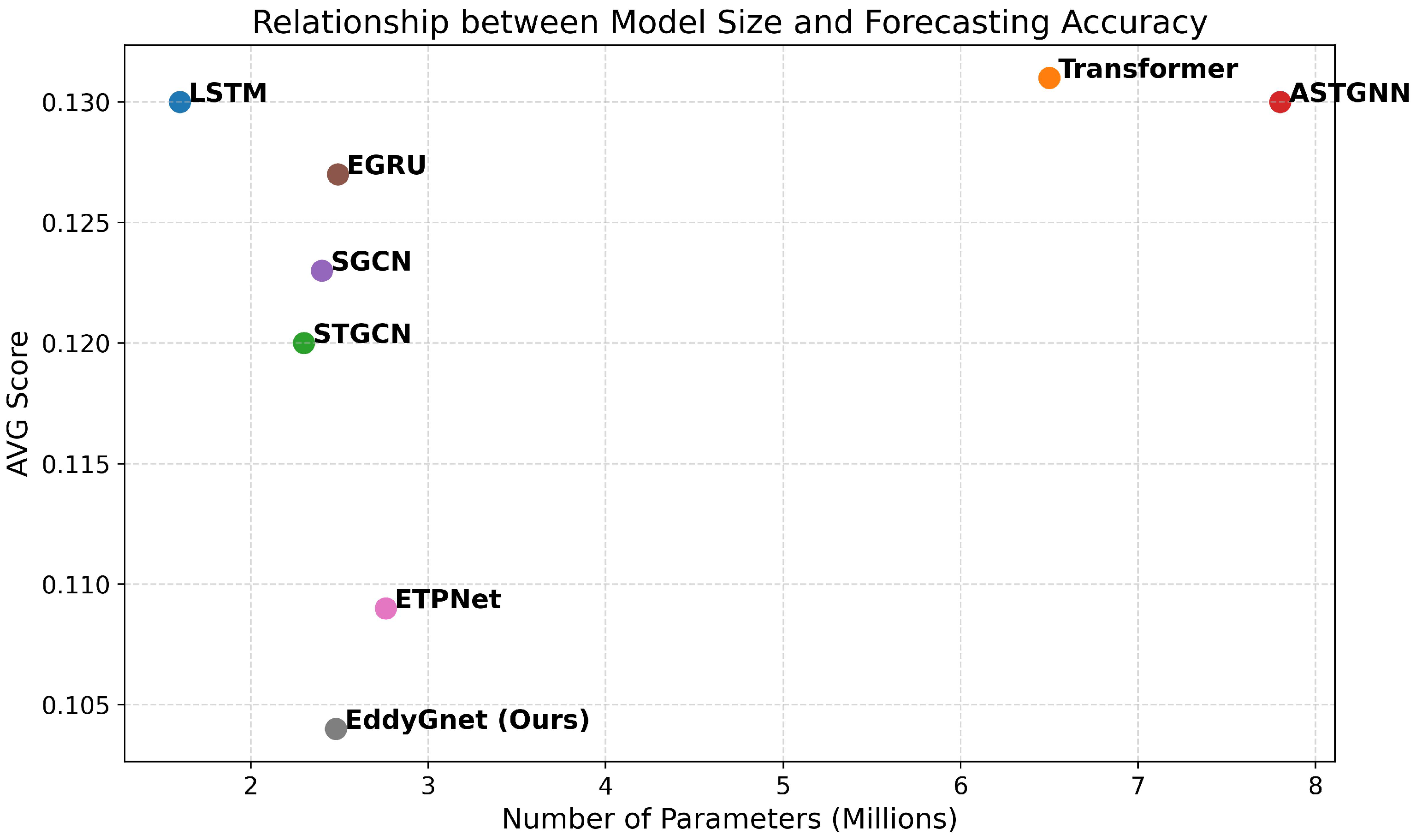
• LSTM and Transformer are classic methods for time-series forecasting. LSTM enhances long-term memory ability through the gating mechanism. Transformer, which is based on the attention mechanism, can directly model dependencies and allows for greater parallelization.
• STGCN, ASTGNN, and SGCN are advanced spatiotemporal forecasting methods that integrate both spatial and temporal information. STGCN employs a 1D CNN for temporal modeling and a GCN for spatial modeling, with a fixed graph structure. ASTGNN utilizes a Transformer for temporal modeling and a graph attention convolutional network (GAN) for spatial modeling, dynamically constructing the graph structure based on node information. SGCN leverages GANs for both spatial and temporal modeling, capturing sparse and directional interactions between nodes.
• EGRU and ETPNet are designed for mesoscale eddy trajectory forecasting. EGRU utilizes the GRU framework from MesoGRU [15], with data processing aligned to the approach presented in this study, and is referred to as EGRU. ETPNet incorporates ocean current data into the LSTM gating units as the “physical constraint”. In the experiment, the dataset described in Section 2.1 is uniformly used.

The results are presented in

Table 1. Comparison of our method with previous approaches on the eddy dataset using data from the past 15 days to predict the next 7 days. The evaluation metrics include MAE, MSE, ADE, and FDE, with lower values indicating better performance.

Model	MAE	MSE	ADE	FDE	AVG
LSTM [22]	0.120	0.058	0.150	0.192	0.130
Transformer [26]	0.124	0.047	0.149	0.204	0.131
STGCN [27]	0.121	0.044	0.139	0.177	0.120
ASTGNN [28]	0.123	0.047	0.147	0.203	0.130
SGCN [29]	0.113	0.038	0.145	0.196	0.123
EGRU [15]	0.119	0.049	0.147	0.191	0.127
ETPNet [18]	0.095	0.039	0.125	0.179	0.109
EddyGnet (Ours)	0.093	0.021	0.124	0.179	0.104

Bold and underlined values indicate the best and second-best performance, respectively.

, evaluated using MAE, MSE, ADE, and FDE metrics. For the 7-day trajectory forecasting, our method outperforms the classic methods in terms of MAE, MSE, and ADE, although it slightly lags behind STGCN in FDE. Overall, our method demonstrates a significant improvement over existing classic methods. On the eddy dataset, our approach offers an average advantage of 4.8% over the second-best method, ETPNet. Figure 7 visualizes the forecasting results of different methods, where we selected trajectories with the same longitude range (${115}^{\circ }$–${117}^{\circ }\mathrm{E}$) but different latitude ranges A and B, as well as trajectories with the same latitude range (${14}^{\circ }$–${15}^{\circ }\mathrm{N}$) but different longitude ranges C and D. These four samples are extracted from randomly shuffled time windows covering a 20-year span, ensuring temporal diversity and validating the model’s generalization performance across varying oceanic conditions.

4. Discussion

4.1. Performance Analysis

As shown in

Table 2. Comparison of forecasting days for different models with a specified accuracy in kilometers.

Model	8 km	9 km	10 km	11 km	12 km	13 km	14 km	15 km
LSTM	0	1	2	3	3	3	3	4
Transformer	0	0	1	1	2	3	3	3
STGCN	0	0	1	2	2	5	6	7
ASTGNN	0	0	2	3	3	3	3	4
SGCN	0	0	2	3	4	4	4	4
EGRU	1	1	2	3	3	3	4	4
ETPNet	0	1	2	3	4	4	5	6
EddyGnet	1	1	2	3	4	4	6	7

Bold values indicate the best performance.

, both EddyGnet and ETPNet maintain a high number of forecast days across all error thresholds, demonstrating superior overall performance. The forecast days of STGCN increase steadily as the error threshold expands, with a notable performance of 7 days at 15 km, indicating strong long-term forecasting ability. However, it performs slightly worse than the first two models in the middle and lower error ranges, suggesting that its forecast error distribution is more balanced. SGCN, EGRU, and LSTM show similar overall performance, with forecast days concentrated in the middle error ranges, indicating limited precision but reasonable stability. In contrast, ASTGNN and Transformer perform significantly worse, with fewer effective forecast days maintained at most error thresholds, especially at 14 km and above, reflecting their difficulty in adapting to long-term forecasting tasks.

EddyGnet outperforms other models in several key aspects, particularly in maintaining effective forecast days in larger error ranges. Unlike models such as LSTM and Transformer, which struggle with long-term stability, EddyGnet consistently maintains effective forecasts up to 7 days in the 15 km error ranges. This strong performance is attributed to its ability to model both dynamic multivariable associations and spatiotemporal interactions between mesoscale eddies, enabling it to better handle the complexities of real-world applications. Compared with other models like STGCN, which performs well in certain error ranges but lacks long-term stability and maintains fewer forecast days at larger error ranges, EddyGnet offers a more reliable solution for long-term trajectory forecasting, providing better adaptability to changing environmental conditions over time.

From Figure 7, it can be observed that methods such as LSTM, Transformer, and EGRU, which consider only the temporal dimension, capture general movement trends but fail to account for the influence of surrounding eddies, leading to suboptimal results. In comparison, SGCN and STGCN with spatiotemporal joint modeling perform relatively well. However, their performance may slightly lag behind because they might fail to accurately capture the complex dynamic associations among the multivariables of mesoscale eddies. ETPNet takes into account the physical constraints of ocean circulation and generally shows good performance. Nevertheless, due to the complex sea conditions caused by the dense eddies in the South China Sea, the physical constraints of ocean circulation may deviate, resulting in its forecasting performance slightly inferior to the method proposed in this paper. Furthermore, we found that traditional recurrent neural network-based methods, such as LSTM and EGRU, exhibit overly small displacements at each time step, resulting in a slower eddy movement process. While these methods retain certain movement trends, they are unable to predict scenarios involving rapid eddy movements.

Notably, the STGCN outperforms our proposed method in terms of the FDE metric. We believe this is due to our adoption of iterated multi-step (IMS) forecasting strategies, where errors accumulate progressively over multiple forecasting steps, leading to suboptimal FDE performance. In contrast, the STGCN employs direct multi-step (DMS) forecasting strategies, which prevent error accumulation at the final time step. However, the DMS approach does not improve overall performance, as the distribution of errors across multiple time steps results in a significantly worse performance in the ADE metric compared with our method.

Additionally, we plotted the uncertainty density of the trajectory forecastings, as shown in Figure 8. The size of each density corresponds to the positional uncertainty of a predicted location. Without correction using the true values, the predicted uncertainty ranges largely encompass the true values. Notably, the location on the 7th day, which experiences the greatest error accumulation, also yields reasonably accurate results, with the overall trend being quite accurate. We successfully estimated an uncertainty density that closely aligns with the true values.

Figure 9 illustrates the forecasting performance of eight models over extended time horizons (7, 14, 21, and 28 days). All models exhibit increasing prediction errors with longer lead times, reflecting the inherent complexity and uncertainty of mesoscale eddy dynamics. EddyGnet consistently outperforms all baseline models at every time step across the 28-day period. This result highlights its superior ability to preserve accuracy over longer forecast spans. Notably, while models like LSTM, STGCN, and EGRU suffer from sharp performance degradation, models such as ETPNet and SGCN show more resilience to extended forecasts, gradually closing the gap with EddyGnet at longer horizons.

These findings confirm the importance of designing trajectory prediction models that are not only accurate in the short term but also robust and generalizable for long-term prediction. EddyGnet’s stable performance suggests that it effectively captures the temporal continuity and spatial evolution patterns necessary for reliable mesoscale eddy forecasting.

To assess the computational efficiency of the proposed method, we measured the model’s training and inference time on an NVIDIA RTX 4060 Ti GPU.

Table 3. Comparison of model complexity, efficiency, performance, and training cost performance.

Model	Params (M)	Train Time (s/Epoch)	Inference Time (ms/Sample)	AVG Score	Train Time × AVG
LSTM	1.6	28	84	0.13	3.64
Transformer	6.5	61	87	0.131	7.99
STGCN	2.3	35	32	0.12	4.2
ASTGNN	7.8	72	89	0.13	9.36
SGCN	2.4	62	41	0.123	7.63
EGRU	2.49	85	79	0.127	10.8
ETPNet	2.76	82	91	0.109	8.94
EddyGnet (Ours)	2.48	68	85	0.104	7.07

Bold and underlined values indicate the best and second-best performance, respectively.

presents a comparison of multiple baseline models, including our proposed EddyGnet.

Although our framework integrates multiple graph learning and attention mechanisms, its computational complexity is well controlled. Specifically, the graph learning module employs sparse adjacency matrices, significantly reducing the computational overhead from matrix multiplications. Additionally, the temporal attention mechanism utilizes a moderate embedding size (64), which keeps the quadratic cost of self-attention within manageable limits. Both the encoder and decoder consist of only one layer, further improving computational efficiency without compromising model expressiveness.

As seen from Table 3, EddyGnet achieves competitive training time (68 s/epoch) and maintains a moderate inference speed (85 ms/sample), even under an iterative multi-step (IMS) prediction strategy. To further compare training efficiency and model performance, we compute the product of training time and prediction error (AVG), which jointly reflects cost-effectiveness. In this metric, EddyGnet ranks third best overall. However, its prediction performance (AVG = 0.104) significantly surpasses that of the two models with better computational efficiency, indicating that our design provides an effective balance between accuracy and efficiency. Although models like LSTM exhibit faster training speed, they yield considerably worse forecasting accuracy. On the other hand, Transformer-based models such as ASTGNN incur larger training costs without gaining accuracy. The training time overhead of EGRU and ETPNet models mainly focuses on complex data fusion. Therefore, EddyGnet offers a strong trade-off, especially in scenarios where moderate computational cost is acceptable in exchange for enhanced forecasting performance.

Figure 10 illustrates the relationship between model size (in millions of parameters) and forecasting accuracy (measured by AVG score) across all baseline methods. Overall, there is no clear linear correlation between model size and accuracy. While larger models such as Transformer and ASTGNN have high parameter counts (over 6 M), their accuracy does not outperform smaller models. For example, STGCN achieves better performance than both with only 2.3 M parameters. Our proposed EddyGnet achieves the best AVG score (0.104) with a moderate parameter size of 2.48 M, demonstrating that an efficient architectural design can outperform brute-force scaling. Models like LSTM and EGRU have small model sizes but fail to deliver competitive forecasting results. This figure highlights the importance of architectural innovation over simply increasing model complexity.

We also note that the use of iterative forecasting (IMS) slightly increases inference latency. In our subsequent ablation studies, we replaced IMS with a direct multi-step (DMS) prediction strategy and conducted a further comparison of performance and computational efficiency.

Beyond computational efficiency, we also evaluate the scalability of the proposed model from multiple perspectives. First, in terms of temporal scalability, the model is trained on nearly 30 years of trajectory data, covering various seasons and interannual variations, which equips it with the ability to handle long-term sequence learning. Second, regarding spatial resolution, since SLA and other physical variables are embedded into node features as trajectory point attributes rather than directly affecting the graph structure, the model can flexibly adapt to higher-resolution input data (e.g., from $0.{25}^{\circ }$ to $0.1^{\circ }$) without structural modification. Third, the model exhibits a modular architecture, including components such as variable embedding, graph convolution, and spatiotemporal attention modules, all of which can be easily replaced or extended—for example, by incorporating additional external variables or enriching feature dimensions—to enhance representation capacity. Lastly, the model design does not rely on region-specific heuristics or prior knowledge, ensuring strong geographic generalization capability and adaptability to a broader range of real-world applications.

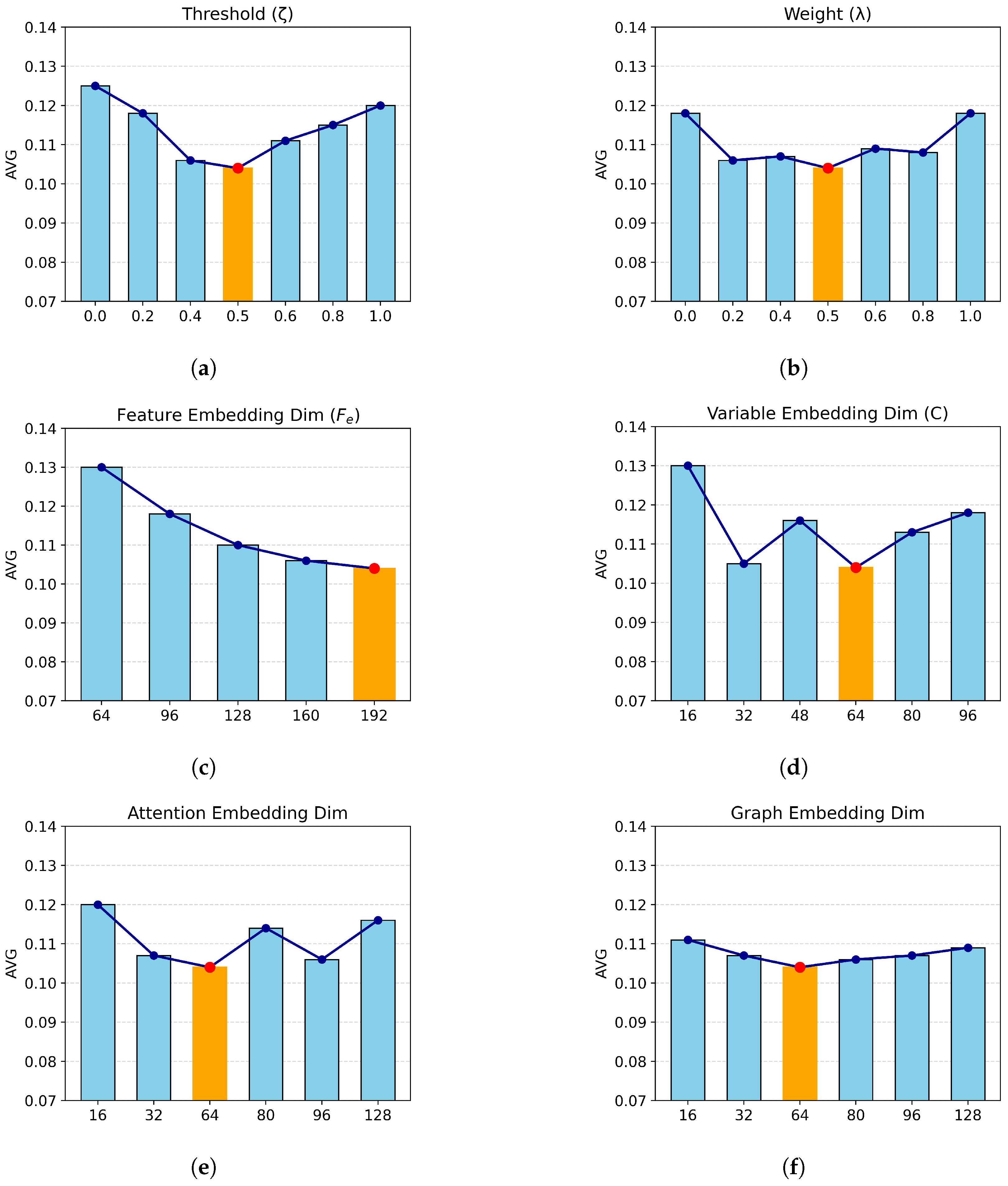
4.2. Parameter Sensitivity Analysis

To evaluate the influence of key hyperparameters on the model’s predictive ability, we conducted sensitivity experiments on six representative hyperparameters, as shown in Figure 11. The evaluation metric is AVG, which represents the average of multiple performance indicators (MSE, MAE, ADE, and FDE), offering a comprehensive assessment of trajectory prediction accuracy.

The threshold $\zeta$ is used to determine whether the interaction between eddies is considered significant. When the metric value between two eddies falls below $\zeta$, their interaction is deemed negligible. Results show that $\zeta =0.5$ yields the best performance. Smaller values (e.g., 0.0 or 0.2) tend to introduce low-relevance connections, increasing noise, whereas larger thresholds (e.g., 0.8 or 1.0) may omit important eddy–eddy relations. The weight $\lambda$ is a coefficient in the loss function that balances the difference in variance between the predicted and true trajectories over the forecasting period. It helps constrain the over-smoothing of predicted trajectories. We observe that setting $\lambda =0.5$ achieves optimal performance, as it maintains the dominance of the main loss while enhancing temporal fluctuation awareness. Very small values overlook variability, while overly large values lead to instability in optimization. The feature embedding dimension $F_e$ determines the latent vector size used to encode individual eddy characteristics. Increasing $F_e$ from 64 to 192 improves performance, with 192 being the upper bound under current GPU constraints. Larger dimensions may further enhance accuracy but at a significant computational cost. The variable embedding dimension C maps each physical variable—including both intrinsic eddy attributes and external environmental factors such as radius, ADT, Ugos, and Vgos—into high-dimensional representations in the multivariate association module. Experimental results indicate that $C=64$ achieves the best trade-off. Smaller values may fail to extract meaningful dependencies, while larger dimensions risk overfitting or redundancy. The attention embedding dimension controls the feature size before the temporal–spatial attention module. Results show noticeable fluctuations across settings, with the optimal performance at 64 dimensions. This implies that the appropriate embedding size is crucial for capturing high-order temporal interactions. Lastly, the graph embedding dimension affects the representation of nodes in the inter-eddy graph. The best performance is also achieved at 64 dimensions, and the results show moderate stability across the tested range, suggesting that while this component contributes to the overall architecture, it is relatively robust to dimensional variations.

In summary, the model exhibits consistent sensitivity to certain hyperparameters—especially threshold, weight, and embedding dimensions. The default values adopted in our experiments (indicated in orange in the figure) are either optimal or close to optimal, validating the rationality and robustness of our parameter selection strategy.

4.3. Ablation Study

To verify the effectiveness of the key components, we conducted an ablation study on the eddy dataset to isolate the contributions of each component to the overall performance, as shown in

Table 4. Ablation study of each component.

Variants	MAE	MSE	ADE	FDE	AVG
wo/MAG Learning	0.110	0.034	0.139	0.189	0.118
wo/Embedding	0.094	0.025	0.126	0.184	0.107
wo/TGL	0.100	0.025	0.130	0.182	0.109
wo/EGL	0.095	0.022	0.125	0.179	0.105
w/L2	0.099	0.030	0.131	0.189	0.112
EddyGnet (Ours)	0.093	0.021	0.124	0.179	0.104

Bold and underlined values indicate the best and second-best performance, respectively.

.

We created five variants of the model as controls by removing the MAG learning module, embedding module, TGL module, and EGL module and by replacing the decayed volatility loss function. From these experiments, we concluded that all components contribute to achieving the best performance to varying degrees. Notably, the results of EddyGnet–MAG Learning, where the MAG learning module was removed, showed a $13\%$ decrease in performance, confirming the importance of learning the evolution of multivariable association graphs in eddy trajectory forecasting. Furthermore, we replaced our loss function, DVLoss, with the traditional $L_2$ loss function. Experimental results showed that the performance decreased by $7.7\%$. This indicates that choosing an appropriate loss function also has a significant impact on the forecasting accuracy of eddy trajectories.

We further explore the impact of downstream predictors on the experimental results. The LSTM predictor adopted in this paper employs an iterative multi-step (IMS) forecasting strategy. We select two direct multi-step (DMS) forecasting strategies as controls, namely, the relatively traditional TCN method and the more advanced Informer decoder which utilizes the attention mechanism. As shown in

Table 5. Comparison study of predictors.

Variants	MAE	MSE	ADE	FDE	AVG	Train Time (s/Epoch)	Inference Time (ms)
w/TCN	0.096	0.025	0.125	0.180	0.107	55	32
w/Informer	0.115	0.042	0.139	0.182	0.120	61	47
w/LSTM + TCN	0.094	0.024	0.124	0.180	0.106	64	58
EddyGnet (Ours)	0.093	0.021	0.124	0.179	0.104	68	85

Bold and underlined values indicate the best and second-best performance, respectively.

, the LSTM predictor employed in this study achieved the best performance. Interestingly, using the more advanced Informer decoder as a predictor led to a $15\%$ decline in performance, which may be attributed to the fact that the Informer has difficulty in processing non-stationary data [30]. The traditional TCN predictor also demonstrated strong forecasting performance, indicating that the upstream model had successfully learned effective feature representations.

To further optimize model performance, we tested a hybrid forecasting approach combining both the LSTM model’s IMS strategy and the TCN model’s DMS strategy. Specifically, the first 3 days are predicted using the LSTM, and the subsequent 7 days are predicted using the TCN. Finally, we select the last 4 days of the TCN prediction as the final result. The hybrid strategy is described by the following formulas:

$$\begin{array}{cc}\hfill Y_{LSTM}& =\mathrm{LSTM}\left(X\right)=[y_1,y_2,y_3]\hfill \end{array}$$

(28)

where $Y_{LSTM}=[y_1,y_2,y_3]$ are the results predicted by LSTM for the first 3 days.

$$\begin{array}{cc}\hfill Y_{TCN}& =\mathrm{TCN}\left(X\right)=[y_1,y_2,y_3,y_4,y_5,y_6,y_7]\hfill \end{array}$$

(29)

where TCN predicts 7 future steps based on the input data X.

$$\begin{array}{cc}\hfill Y_{LSTM+TCN}& =[y_1,y_2,y_3,y_4,y_5,y_6,y_7]\hfill \end{array}$$

(30)

where $Y_{LSTM+TCN}$ is the final prediction, combining the first 3 days from LSTM and the last 4 days from TCN.

In Table 5, we compared the results of the hybrid strategy with those of the pure **LSTM model’s IMS strategy** and **TCN model’s DMS strategy**. The experimental results showed that the hybrid strategy did not significantly improve forecasting performance, and the final performance was similar to that of using the **LSTM model’s IMS strategy** alone. This suggests that while LSTM performed well in the short-term forecast, combining it with the **TCN model’s DMS strategy** did not bring the expected improvement.

In addition to prediction accuracy, we further analyzed the inference and training efficiency of each downstream predictor. As shown in Table 5, direct multi-step predictors like TCN and Informer reduce inference latency significantly (to 32 ms and 47 ms, respectively), compared with LSTM’s 85 ms. However, this comes with a noticeable decline in forecasting accuracy, especially in the case of Informer. The proposed hybrid predictor (LSTM + TCN) achieves a good balance between efficiency and accuracy, reducing inference time to 58 ms while maintaining competitive performance (AVG = 0.106). The training time is also moderate (64 s/epoch), which demonstrates its practical value for scenarios requiring lower latency without sacrificing too much accuracy. These results indicate that the selection of a forecasting strategy can be adjusted based on specific application requirements: IMS (LSTM) for high-accuracy tasks, DMS (TCN) for faster inference, and hybrid strategies for balanced performance.

To better forecast mesoscale eddy trajectories, it is essential to incorporate not only coordinate sequences but also relevant physical variables that reflect the oceanic environment and the characteristics of the eddies themselves. In this section, we analyze the rationality and effectiveness of the auxiliary variables used in our model.

Our variable selection is grounded in well-established principles of physical oceanography. Specifically, we include two categories of variables: (1) eddy-intrinsic attributes such as amplitude, radius, average speed of the eddies’ contours, and average velocity of the eddies’ centers and (2) surrounding environmental conditions, including absolute dynamic topography (ADT), and both the zonal (u) and meridional (v) components of the absolute geostrophic velocity at the sea surface. The eddy attributes originate from the same AVISO MET dataset as the eddy trajectory coordinates, ensuring consistency and accuracy in spatiotemporal resolution. Prior studies [31,32] have demonstrated that amplitude and radius represent the eddy’s geometric strength and scale, while the average speed of the eddies’ contours and average velocity of the eddies’ centers directly influence its drifting behavior. These factors are closely linked to trajectory evolution and have been widely used in eddy tracking and analysis. The environmental variables, obtained from the Copernicus Marine Environment Monitoring Service (CMEMS), provide the broader ocean background that influences eddy movement. ADT reflects the sea surface height above the geoid and indicates the baroclinic pressure gradients that steer mesoscale eddies. The absolute geostrophic velocity components represent large-scale ocean circulation, contributing to the advective motion of eddies [33].

To evaluate the contribution of environmental variables, we conducted a set of ablation experiments. As shown in

Table 6. Ablation study on the physical oceanographic variables.

Variant	MAE	MSE	ADE	FDE	AVG
w/o ADT	0.096	0.025	0.129	0.184	0.109
w/o GeoVel (u/v)	0.097	0.026	0.130	0.185	0.110
w/o All Physics	0.099	0.028	0.132	0.189	0.112
EddyGnet (Ours)	0.093	0.021	0.124	0.179	0.104

Bold and underlined values indicate the best and second-best performance, respectively.

, removing individual environmental variables led to noticeable performance degradation. Specifically, removing ADT increased the average error (AVG) from 0.104 to 0.109, while removing the geostrophic velocity components raised the AVG to 0.110. When all environmental variables were removed, the AVG error further increased to 0.112. These results validate that the environmental variables significantly enhance the forecasting ability of our model.

Collectively, the inclusion of both eddy-intrinsic and environmental variables is physically grounded and empirically effective, reinforcing the importance of physically informed learning in ocean prediction tasks.

To investigate the relative contribution of each input variable to coordinate forecasting, we applied SHAP (SHapley Additive exPlanations) [34] analysis and computed the feature importance scores based on the trained EddyGnet model. As illustrated in Figure 12, the current longitude and latitude of the eddy centers exhibit the highest contributions (0.31 and 0.30, respectively), which aligns with the intuitive understanding that spatial continuity plays a crucial role in predicting future positions. In addition, the average velocities of the eddy center (0.11) and angular difference (0.08) show considerable influence, highlighting the importance of dynamic properties in capturing the propagation behavior of eddies.

Among the physical oceanic variables, absolute dynamic topography (ADT) and the zonal and meridional components of geostrophic surface velocity contribute 6.5%, 4.6%, and 4.8%, respectively. These values confirm the physical relevance of these variables.

5. Summary

We propose a framework that integrates MAG learning and STEAG learning, contributing to mesoscale eddy trajectory forecasting. Our approach represents the complex inter-relations among multiple variables of eddies, such as position coordinates, effective radius, velocity, and amplitude, using graph nodes and edges. Specifically, we divide the data into multiple time segments and extract statistical information, such as the mean and variance of each variable within a segment, to represent graph nodes. The inter-variable associations are modeled as graph edges. By transferring information across historical time segments, the framework captures the temporal evolution of the multivariable association graph, enabling dynamic and accurate modeling of multivariable associations. Furthermore, we design a STEAG learning module for mesoscale eddy forecasting. It constructs a spatiotemporal graph to represent complex spatiotemporal associations. It models the temporal dependencies of mesoscale eddy trajectories using a directed temporal graph and the interactions between eddies using a directed spatial graph. Specifically, we employ an attention mechanism to learn the interaction weights among trajectory points, further pruning redundant interaction information. Finally, to mitigate error accumulation caused by high initial forecasting errors and handle the fluctuations of the data, we design a decayed volatility loss function. Using the AVISO dataset, we select the South China Sea, a region characterized by complex and dense eddies, for the experiment. Extensive experiments and various evaluation methods demonstrate that the proposed eddy trajectory forecasting framework outperforms existing classic methods, achieving an average forecasting error of less than 14 km over a 7-day forecast period.

It is important to acknowledge that it comes with certain drawbacks. The main limitation of this study is that our model lacks oceanic physical mechanisms to consider the direct impacts of ocean environmental factors on eddy trajectories, which leads to insufficient interpretability of the model. In future work, we plan to rationally incorporate physical mechanisms and prior knowledge into the training process of the model so as to further enhance the predictive performance and interpretability of the model.

References

1. Morrow, R.; Church, J.; Coleman, R.; Chelton, D.; White, N. Eddy momentum flux and its contribution to the Southern Ocean momentum balance. Nature 1992, 357, 482–484. [Google Scholar] [CrossRef]
2. Lin, Y.; Wang, G. The effects of eddy size on the sea surface heat flux. Geophys. Res. Lett. 2021, 48, e2021GL095687. [Google Scholar] [CrossRef]
3. Zhang, Z.; Wang, W.; Qiu, B. Oceanic mass transport by mesoscale eddies. Science 2014, 345, 322–324. [Google Scholar] [CrossRef] [PubMed]
4. Chen, G.; Han, G. Contrasting short-lived with long-lived mesoscale eddies in the global ocean. J. Geophys. Res. Oceans 2019, 124, 3149–3167. [Google Scholar] [CrossRef]
5. Martínez-Moreno, J.; Hogg, A.M.; England, M.H.; Constantinou, N.C.; Kiss, A.E.; Morrison, A.K. Global changes in oceanic mesoscale currents over the satellite altimetry record. Nat. Clim. Change 2021, 11, 397–403. [Google Scholar] [CrossRef]
6. van Westen, R.M.; Dijkstra, H.A. Ocean eddies strongly affect global mean sea-level projections. Sci. Adv. 2021, 7, eabf1674. [Google Scholar] [CrossRef] [PubMed]
7. Beech, N.; Rackow, T.; Semmler, T.; Danilov, S.; Wang, Q.; Jung, T. Long-term evolution of ocean eddy activity in a warming world. Nat. Clim. Change 2022, 12, 910–917. [Google Scholar] [CrossRef]
8. Horvat, C.; Tziperman, E.; Campin, J.M. Interaction of sea ice floe size, ocean eddies, and sea ice melting. Geophys. Res. Lett. 2016, 43, 8083–8090. [Google Scholar] [CrossRef]
9. Goldstein, E.D.; Pirtle, J.L.; Duffy-Anderson, J.T.; Stockhausen, W.T.; Zimmermann, M.; Wilson, M.T.; Mordy, C.W. Eddy retention and seafloor terrain facilitate cross-shelf transport and delivery of fish larvae to suitable nursery habitats. Limnol. Oceanogr. 2020, 65, 2800–2818. [Google Scholar] [CrossRef]
10. Chelton, D.B.; Schlax, M.G.; Samelson, R.M.; de Szoeke, R.A. Global observations of large oceanic eddies. Geophys. Res. Lett. 2007, 34, L15606. [Google Scholar] [CrossRef]
11. Shriver, J.; Hurlburt, H.E.; Smedstad, O.M.; Wallcraft, A.J.; Rhodes, R.C. 1/32 real-time global ocean prediction and value-added over 1/16 resolution. J. Mar. Syst. 2007, 65, 3–26. [Google Scholar] [CrossRef]
12. Masina, S.; Pinardi, N. Mesoscale data assimilation studies in the Middle Adriatic Sea. Cont. Shelf Res. 1994, 14, 1293–1310. [Google Scholar] [CrossRef]
13. Ma, C.; Li, S.; Wang, A.; Yang, J.; Chen, G. Altimeter observation-based eddy nowcasting using an improved Conv-LSTM network. Remote Sens. 2019, 11, 783. [Google Scholar] [CrossRef]
14. Wang, X.; Wang, H.; Liu, D.; Wang, W. The prediction of oceanic mesoscale eddy properties and propagation trajectories based on machine learning. Water 2020, 12, 2521. [Google Scholar] [CrossRef]
15. Wang, X.; Wang, X.; Yu, M.; Li, C.; Song, D.; Ren, P.; Wu, J. MesoGRU: Deep learning framework for mesoscale eddy trajectory prediction. IEEE Geosci. Remote Sens. Lett. 2021, 19, 1–5. [Google Scholar] [CrossRef]
16. Nian, R.; Cai, Y.; Zhang, Z.; He, H.; Wu, J.; Yuan, Q.; Geng, X.; Qian, Y.; Yang, H.; He, B. The identification and prediction of mesoscale eddy variation via memory in memory with scheduled sampling for sea level anomaly. Front. Mar. Sci. 2021, 8, 753942. [Google Scholar] [CrossRef]
17. Wang, X.; Li, C.; Wang, X.; Tan, L.; Wu, J. Spatio–temporal attention-based deep learning framework for mesoscale eddy trajectory prediction. IEEE J. Sel. Top. Appl. Earth Obs. Remote Sens. 2022, 15, 3853–3867. [Google Scholar] [CrossRef]
18. Ge, L.; Huang, B.; Chen, X.; Chen, G. Medium-range trajectory prediction network compliant to physical constraint for oceanic eddy. IEEE Trans. Geosci. Remote Sens. 2023, 61, 4206514. [Google Scholar] [CrossRef]
19. Zhang, X.; Huang, B.; Chen, G.; Ge, L.; Radenkovic, M.; Hou, G. Global oceanic mesoscale eddies trajectories prediction with knowledge-fused neural network. IEEE Trans. Geosci. Remote Sens. 2024, 62, 4205214. [Google Scholar] [CrossRef]
20. Tang, H.; Lin, J.; Ma, D. Direct prediction for oceanic mesoscale eddy geospatial distribution through prior statistical deep learning. Expert Syst. Appl. 2024, 249, 123737. [Google Scholar] [CrossRef]
21. Long, S.; Tian, F.; Ma, Y.; Cao, C.; Chen, G. “Gear-like” process between asymmetric dipole eddies from satellite altimetry. Remote Sens. Environ. 2024, 314, 114372. [Google Scholar] [CrossRef]
22. Graves, A.; Graves, A. Long short-term memory. In Supervised Sequence Labelling with Recurrent Neural Networks; Springer: Berlin/Heidelberg, Germany, 2012; pp. 37–45. [Google Scholar]
23. Bai, S.; Kolter, J.Z.; Koltun, V. An empirical evaluation of generic convolutional and recurrent networks for sequence modeling. arXiv 2018, arXiv:1803.01271. [Google Scholar] [CrossRef]
24. Raksincharoensak, P.; Hasegawa, T.; Nagai, M. Motion planning and control of autonomous driving intelligence system based on risk potential optimization framework. Int. J. Automot. Eng. 2016, 7, 53–60. [Google Scholar] [CrossRef] [PubMed]
25. Alahi, A.; Goel, K.; Ramanathan, V.; Robicquet, A.; Fei-Fei, L.; Savarese, S. Social lstm: Human trajectory prediction in crowded spaces. In Proceedings of the IEEE Conference on Computer Vision and Pattern Recognition, Las Vegas, NV, USA, 27–30 June 2016; pp. 961–971. [Google Scholar]
26. Vaswani, A. Attention is all you need. In Advances in Neural Information Processing Systems; The MIT Press: Cambridge, MA, USA, 2017. [Google Scholar]
27. Yu, B.; Yin, H.; Zhu, Z. Spatio-temporal graph convolutional networks: A deep learning framework for traffic forecasting. arXiv 2017, arXiv:1709.04875. [Google Scholar]
28. Guo, S.; Lin, Y.; Wan, H.; Li, X.; Cong, G. Learning dynamics and heterogeneity of spatial-temporal graph data for traffic forecasting. IEEE Trans. Knowl. Data Eng. 2021, 34, 5415–5428. [Google Scholar] [CrossRef]
29. Shi, L.; Wang, L.; Long, C.; Zhou, S.; Zhou, M.; Niu, Z.; Hua, G. SGCN: Sparse graph convolution network for pedestrian trajectory prediction. In Proceedings of the IEEE/CVF Conference on Computer Vision and Pattern Recognition, Nashville, TN, USA, 20–25 June 2021; pp. 8994–9003. [Google Scholar]
30. Shen, L.; Wei, Y.; Wang, Y. GBT: Two-stage transformer framework for non-stationary time series forecasting. Neural Netw. 2023, 165, 953–970. [Google Scholar] [CrossRef] [PubMed]
31. Chlorophyll, O. The Influence of Nonlinear Mesoscale Eddies on Near-Surface. Science 2011, 1208897, 334. [Google Scholar]
32. Faghmous, J.H.; Frenger, I.; Yao, Y.; Warmka, R.; Lindell, A.; Kumar, V. A daily global mesoscale ocean eddy dataset from satellite altimetry. Sci. Data 2015, 2, 150028. [Google Scholar] [CrossRef] [PubMed]
33. Liu, T.; Abernathey, R. A global Lagrangian eddy dataset based on satellite altimetry. Earth Syst. Sci. Data Discuss. 2023, 15, 1765–1778. [Google Scholar] [CrossRef]
34. Lundberg, S.M.; Lee, S.I. A unified approach to interpreting model predictions. In Advances in Neural Information Processing Systems; The MIT Press: Cambridge, MA, USA, 2017; Volume 30, pp. 4768–4777. [Google Scholar]
Figure 1. Illustration of mesoscale eddy evolution and multivariable variations over time (T1–T4: time step 1 to time step 4). Radius: the radius of the fit circle corresponding to the contour; amplitude: the height difference between the eddies’ center and contour; velocity: the moving average velocity of the eddies’center; Ugos: absolute geostrophic velocity of sea surface: zonal component; and Vgos: absolute geostrophic velocity of sea surface: meridian component.
Remotesensing 17 02524 g001
Figure 2. Overall framework of the model.
Remotesensing 17 02524 g002
Figure 3. Eddy multivariable association graph. In the ξ 1 time segment, velocity is positively correlated with amplitude, while displacement is negatively correlated with effective radius. However, in the ξ 2 time segment, the correlation between velocity and amplitude becomes negative, and the correlation between displacement and effective radius weakens.
Remotesensing 17 02524 g003
Figure 4. Graph Learning Network (GLN).
Remotesensing 17 02524 g004
Figure 5. Temporal and eddy graph learning modules.
Remotesensing 17 02524 g005
Figure 6. Training and Validation Loss. Training Loss represents the value calculated using the DVLoss function for the real values and the predicted values on the training set. Validation Loss refers to the average value computed with four evaluation metrics, namely, MAE (Mean Absolute Error), MSE (Mean Squared Error), ADE (Average Displacement Error), and FDE (Final Displacement Error), for the real values and the predicted values on the validation set.
Remotesensing 17 02524 g006
Figure 7. Visualization of forecasting results from different models. Each group contains a main trajectory map with SLA background (top) and four subplots (bottom) showing the predicted positions at specific forecast steps. The subplots correspond to T1, T3, T5, and T7—representing the 1st, 3rd, 5th, and 7th predicted time steps, respectively. Groups (a,b) depict trajectories within the same longitude range (115°–117°E) but varying latitude ranges. Groups (c,d) depict trajectories within the same latitude range (14°–15°N) but different longitude ranges.
Remotesensing 17 02524 g007
Figure 8. Temporal estimated densities by our method. T1, T3, T5, and T7 denote the forecast time steps.
Remotesensing 17 02524 g008
Figure 9. Comparison of prediction accuracies (AVG scores) over increasing forecast horizons (7, 14, 21, and 28 days). EddyGnet demonstrates the most stable performance across all time lengths, highlighting its robustness in long-term eddy trajectory forecasting.
Remotesensing 17 02524 g009
Figure 10. Relationship between model size and forecasting accuracy (AVG score).A lower AVG score indicates better performance.
Remotesensing 17 02524 g010
Figure 11. Parameter sensitivity analysis under different hyperparameter configurations, evaluated using the average performance (AVG). (a) Threshold ζ controls the influence threshold of eddy interactions, where lower correlation values are filtered out; (b) weight λ is the coefficient for balancing trajectory variance loss, used to penalize over-smoothed predictions; (c) feature embedding dimension F e determines the hidden size of the trajectory encoder–decoder structure; (d) variable embedding dimension C governs how many neurons each auxiliary variable is projected to before interaction; (e) attention embedding dimension affects the representation capacity before attention-based spatiotemporal fusion; and (f) graph embedding dimension controls the representation scale in the graph-based convolutional module. Each curve shows how performance fluctuates when one hyperparameter is changed while others are fixed. The orange bar and red marker indicate the configuration used in our final model.
Remotesensing 17 02524 g011
Figure 12. Estimated SHAP values.
Remotesensing 17 02524 g012