Article

Estimation of Tree Diameter at Breast Height (DBH) and Biomass from Allometric Models Using LiDAR Data: A Case of the Lake Broadwater Forest in Southeast Queensland, Australia

1
School of Surveying and Built Environment, University of Southern Queensland, Toowoomba, QLD 4350, Australia
2
School of Surveying and Built Environment, University of Southern Queensland, Springfield, QLD 4300, Australia
*
Author to whom correspondence should be addressed.
Remote Sens. 2025, 17(14), 2523; https://doi.org/10.3390/rs17142523 (registering DOI)
Submission received: 1 June 2025 / Revised: 16 July 2025 / Accepted: 17 July 2025 / Published: 20 July 2025

Abstract

Light Detection and Ranging (LiDAR) provides three-dimensional information that can be used to extract tree parameter measurements such as height (H), canopy volume (CV), canopy diameter (CD), canopy area (CA), and tree stand density. LiDAR data does not directly give diameter at breast height (DBH), an important input into allometric equations to estimate biomass. The main objective of this study is to estimate tree DBH using existing allometric models. Specifically, it compares three global DBH pantropical models to calculate DBH and to estimate the aboveground biomass (AGB) of the Lake Broadwater Forest located in Southeast (SE) Queensland, Australia. LiDAR data collected in mid-2022 was used to test these models, with field validation data collected at the beginning of 2024. The three DBH estimation models—the Jucker model, Gonzalez-Benecke model 1, and Gonzalez-Benecke model 2—all used tree H, and the Jucker and Gonzalez-Benecke model 2 additionally used CD and CA, respectively. Model performance was assessed using five statistical metrics: root mean squared error (RMSE), mean absolute error (MAE), mean absolute percentage error (MAPE), percentage bias (MBias), and the coefficient of determination (R2). The Jucker model was the best-performing model, followed by Gonzalez-Benecke model 2 and Gonzalez-Benecke model 1. The Jucker model had an RMSE of 8.7 cm, an MAE of −13.54 cm, an MAPE of 7%, an MBias of 13.73 cm, and an R2 of 0.9005. The Chave AGB model was used to estimate the AGB at the tree, plot, and per hectare levels using the Jucker model-calculated DBH and the field-measured DBH. AGB was used to estimate total biomass, dry weight, carbon (C), and carbon dioxide (CO2) sequestered per hectare. The Lake Broadwater Forest was estimated to have an AGB of 161.5 Mg/ha in 2022, a Total C of 65.6 Mg/ha, and a CO2 sequestered of 240.7 Mg/ha in 2022. These findings highlight the substantial carbon storage potential of the Lake Broadwater Forest, reinforcing the opportunity for landholders to participate in the carbon credit systems, which offer financial benefits and enable contributions to carbon mitigation programs, thereby helping to meet national and global carbon reduction targets.

1. Introduction

Accurate biomass estimation plays a crucial role in forestry management, serving as the foundation of the timber industry [1,2]. It is essential for ecological studies and supports multiple disciplines, including forest productivity, energy dynamics, carbon and nitrogen cycles, nutrient flow, and forest ecosystem analysis [1,3,4]. Forests act as the largest terrestrial carbon reserves, containing over 80% of aboveground carbon (AGC) and more than 70% of soil organic carbon (SOC) [4,5]. They contribute significantly to carbon sequestration, capturing atmospheric carbon and storing it in biomass and soil, a vital process for regulating the global carbon cycle [6]. Traditionally, biomass studies focused on timber quality and production; however, with increasing concerns about climate change and greenhouse gas emissions, carbon sequestration has gained significant attention [7]. Consequently, precise and timely biomass monitoring is essential for understanding climate change impacts on carbon sinks and developing policies to mitigate environmental changes [1].
Direct and indirect methods are the two main approaches commonly used under the Intergovernmental Panel on Climate Change (IPCC), Tier 2 and Tier 3, to estimate biomass [8,9]. Direct or destructive methods require felling individual trees to measure the weight of stems, branches, and leaves, followed by drying to determine their final dry weight [10,11]. The direct method is highly time-consuming and labor-intensive, posing potential risks to flora and fauna, particularly where large trees or tree roots are sampled [12]. However, the destructive sampling approach is the most accurate method. Direct sampling also provides reliable input data to construct robust allometric equations [13]. In contrast, indirect methods rely on inventory data without damaging trees [11]. The commonly collected data includes tree diameter at breast height (DBH) (1.3 m) and tree height (H) within sample plots, with biomass subsequently estimated using allometric equations [14]. Allometric equations are mathematical formulas that relate biomass to tree attributes such as tree height (H), diameter at breast height (DBH), wood density (ρ), canopy diameter (CD), canopy area (CA), canopy height (CH), and canopy volume (CV) [15,16]. Developing new or improved species-specific allometric equations is always preferable to indirect methods (described as Tier 2 above) [17].
Remote sensing techniques, such as Light Detection and Ranging (LiDAR), offer an alternative or complementary approach to traditional field methods by providing comprehensive forest structure data across both vertical and horizontal dimensions at a landscape scale [18,19]. LiDAR as a remote sensing technique is well suited for characterizing various tree attributes, such as H, CA, CD, CV, CH, leaf area, and aboveground biomass [20,21,22,23,24]. Recently, there has been a shift toward utilizing remote sensing as the primary method for monitoring forest carbon [25,26,27,28]. Remote sensing techniques are more efficient and less labor-intensive than traditional field methods, offering the advantage of estimating forest characteristics across broader spatial and temporal scales [29]. Although LiDAR is effective in estimating various individual tree parameters with high accuracy, it does not directly measure tree DBH [30,31]. Therefore, to estimate aboveground biomass (AGB) using LiDAR, it is essential to apply equations that derive tree DBH from other measured tree and stand variables, as most individual tree biomass equations rely on DBH as a key input [32,33,34]. Numerous diameter–height equations have been documented in forestry literature concerning LiDAR applications [35,36]. Some of these equations estimate diameter solely from LiDAR-derived tree height, while others incorporate additional predictor variables such as crown diameter or tree age [37]. Typically, these equations are linear or can be converted into linear forms using power or exponential functions, and when their inverses exist, diameter becomes the dependent variable, while tree height serves as the predictor variable in the transformed equations [37].
This study aimed to assess the performance of three selected pantropical global DBH models by utilizing airborne LiDAR data in forest environments, with Lake Broadwater Forest in SE Queensland, Australia, as the case study. This research study evaluated two diameter calculation models listed in Gonzalez-Benecke, Fernández [38] and one in Jucker, Caspersen [39] to estimate the DBH of the Lake Broadwater Forest. The models were developed to be applicable across different environments, tree species, and a wide range of tree sizes. Gonzalez-Benecke, Fernández [38] used two models: the first model, where H is known, and the second model, where H and CA are known. These models were selected for this project because they were developed using tree species, specifically Pinus radiata, which closely resemble the predominant species found in the study area (white cypress pine). Jucker, Caspersen [39], the third model used in this study, employed a simple metric combining two allometric dimensions, H and CD, to derive a universal equation for estimating stem diameter, which proved robust across a wide range of tree sizes, forest types, and species. The specific objectives of this study were (1) to evaluate the accuracy of published allometric models in estimating DBH for individual trees using LiDAR-derived measurements, including tree height, crown diameter, and crown area; (2) to assess the performance of these DBH models using statistical metrics; and (3) to identify the best-performing DBH model and estimate the biomass of the study area. The methodological contribution and practical implementation of this study will be particularly useful for landowners (including farmers) and mining companies in the region to use this methodology to estimate total biomass and subsequently estimate carbon and CO2 sequestered by their forests. This will enable them to benefit financially from the Australian Carbon Credit Units market. Landowners must engage in climate change mitigation efforts to help the nation achieve its climate change targets. Landowners, including farmers, can also use this method to estimate the individual tree thickness or diameter and identify merchantable trees in their forests using freely available LiDAR data from various repositories.

2. Materials and Methods

2.1. Study Area

The study area covers Lake Broadwater Forest, which is situated approximately 25 km southwest of Dalby town in Western Downs Regional Council, in Queensland, Australia. The geographical coordinates are 27°21′16.3″S 151°06′18.0″E. It falls under the GDA 2020/MGA Zone 56 projected coordinate system, with approximate coordinates ranging from (310,865 m E/6,970,898 m N; 316,062 m E/6,976,070 m N) (Figure 1) according to the Australian Geospatial Reference System. Lake Broadwater forest mainly comprises white cypress pine (Callitris glaucophylla) on higher ground, brigalow (Acacia harpophylla) along the main Lake Broadwater highway, and narrow-leaved ironbark (Eucalyptus crebra) scattered throughout the whole forest. River red gum (Eucalyptus camaldulensis) occurs along the riparian wetlands and along the lake shoreline. Lake Broadwater, encompassing a 1212-hectare conservation park, is situated within one of Queensland’s most extensively farmed agricultural regions to attract visitors. It is included in the Directory of Important Wetlands in Australia and serves as an outstanding example of a semi-permanent freshwater lake, a rare characteristic in this region. The lake fills only following heavy rainfall events and, when completely inundated, attains a depth of 3 to 4 m. It undergoes periodic drying, which can sometimes persist for extended durations [40].
According to the Department of Environment, Science and Innovation (DETSI) [40], the park conserves valuable remnants of the vegetation types that historically dominated the Western Downs prior to European settlement, many of which have become rare due to agricultural development. The park is home to over 450 recorded plant species. The open-water and lake-edge communities are regarded as the most ecologically significant among the four identified wetland communities surrounding the lake.
Various species dominate the open-water zone, including shiny nardoo (Marsilea mutica), swamp lily (Ottelia ovalifolia), native water hyacinth (Monochoria cyanea), and ribbon weed (Vallisneria gigantea) [40]. The lake edge zone is primarily dominated by river red gum (Eucalyptus camaldulensis), which forms a canopy over an understory of grasses and sedges, including Leptochloa, Cyperus, and Polygonum spp. Figure 2 shows some of the trees in the study area.
Eucalypt forests and woodlands containing blue gum (Eucalyptus tereticornis), narrow-leaved red ironbark (Eucalyptus crebra), poplar box (Eucalyptus populnea), and narrow-leaved grey box (Eucalyptus woollsiana) grow on the flat plains and low ridges in the vicinity of the lake. Dense patches of white cypress pine (Callitris glaucophylla) and brigalow (Acacia harpophylla) are in areas with appropriate soils, while wilga trees (Geijera parviflora) are frequently present. It has to be noted that the trees in the Australian forests are not deciduous trees that shed leaves in winter but are semi-evergreen and dry sclerophylls, which rarely shed their leaves except during severe dry periods [41,42].

2.2. LiDAR Data Collection

The 2022 LiDAR data used in this research were collected by Arrow Energy, a coal seam gas company in Queensland, Australia, and accessed in the standard LAS file format. The LiDAR data collection was part of the Arrow Surat-wide survey that covered an area of approximately 4643 km2 to monitor potential subsidence over the Surat Gas project. The LiDAR survey was conducted in winter from 13 June to 7 August 2022. Aerial imagery capture was carried out by Aerometric, Aero Photogrammetry, and Mapping (AAM, SA, Sydney, Australia, a subsidiary of Woolpert Company), a geophysics company. The LiDAR survey was conducted using the Optech Galaxy 473 sensor (Teledyne Optec, Toronto, ON, Canada) with a scan angle of 29 degrees. The laser scan rate was 450 kHz with a pulse repetition frequency of 40 Hz. The LiDAR data had a horizontal spatial accuracy of +/−0.10 m and vertical spatial accuracy of +/−0.05 m @ 68% confidence interval (CI). The point density was 4 ppsm. The data had a horizontal datum of GDA2020 and a vertical datum of Australian Height Datum (AHD) with Ausgeoid2020 geoid model. The aerial LiDAR survey was planned to achieve +/−5 cm vertical accuracy with an emitted density of 10 ppsm or better to attain a ground return of +4 ppsm with classification to ICSM level 2. Red-Green-Blue (RGB) Imagery products with a ground sampling distance (GSD) of 10 cm were generated from simultaneously captured imagery with a planned accuracy of better than 2 Px (RMS). High-precision GNSS and inertial measurement unit (IMU) systems were used to georeference the data, and the ground control points were established using a high-precision GNSS observation procedure from 5 September to 24 September 2022 for calibration and validation.

2.3. Field Measurements

Forest circular plots, each approximately 1256 m2 in size with a radius of 20 m, were selected from different parts of the Lake Broadwater Forest based on tree density, tree species, and accessibility. Field surveys were conducted in March 2024 over a three-day period to collect validation data. A Garmin GPS Map 67 i handheld GNSS receiver (Sijhih City, Taiwan) was used to locate the center of the selected plots and to confirm the location of certain selected trees that were used for detailed validation of parameters derived from the LiDAR data, such as tree height, DBH, and canopy measurements (canopy width E-W, N-S direction, and canopy area). The X, Y, and Z coordinates of a few selected trees, primarily located on Plot 6, were recorded with positional accuracy ranging from 2 m to 3 m, depending on the tree canopy cover, which blocked the satellite signals. A smartphone compass and tape measure were used to resolve GNSS satellite connectivity issues. Tree species identification was recorded, and DBH measurements were obtained using a tree caliper at 1.3 m above the tree stem. An attempt to measure representative tree heights and crown diameters in the field was unsuccessful; therefore, no field height measurements and canopy dimensions were used in the data validation process. Instead, individual trees were located and delineated from LiDAR-derived canopy height models (CHMs), and crown-level metrics (e.g., crown volume and projected area) were computed from the LiDAR 3-D point cloud.
Google Maps Satellite imagery was also used to identify the locations of the trees. Using the 2022 LiDAR dataset and satellite imagery, twenty-one plots were initially identified in the office as potential validation sites, and seven were finally selected for data collection (Table 1). The table shows an average of 61 trees per plot, 481 trees per hectare, a tree height average of 18 m, a crown diameter (CD) average of 4 m, crown diameter north_south (CD N_S) average of 3.8 m, crown diameter east_west (CD E_W) average of 3.8 m, a crown area (CA) average of 13 m2, and a crown volume (CV) average of 28 m3. A field reconnaissance survey was conducted on most of the 21 initially selected plots, resulting in the final selection of 8 plots deemed most suitable for data collection, based on accessibility and tree species distribution. Field measurements were collected from a total of 408 trees across seven plots.

2.4. Data Analysis

The 2022 LiDAR point cloud data were processed using ArcGIS 2.3.0 Pro and LiDAR 360 v8.0 software to generate individual tree parameters, digital elevation models (DEMs), and digital surface models (DSMs). Canopy height models (CHMs) were generated by subtracting the DEM from the DSM raster image datasets, following the methodology suggested by [43,44]. Field validation data were collected for model evaluation, and various statistical models were generated to estimate DBH. Three DBH estimation models were compared against field-measured data to determine the most accurate predictive model. Figure 3 shows a simplified data processing workflow in ArcGIS and LiDAR360, where a digital CHM [45] was the final product from which tree parameters were derived. This image is called the Height Above Ground Level (HAGL) and can be used to calculate biomass using allometric equations [46]. The LiDAR data were imported into both ArcGIS Pro and LiDAR 360 software, where they were processed with different filtering algorithms and classified to produce the DCM and DSM raster images. Filtering LiDAR point cloud data is a crucial step in deriving accurate raster images. ArcGIS Pro includes tools within the 3D Analyst and LAS Dataset toolsets to perform these filtering operations but doesn’t explicitly expose algorithm names; however, it provides automated tools that apply internal algorithms [47]. LiDAR360 point cloud filtering algorithms are more transparent and advanced than in ArcGIS Pro. Three filtering algorithms for ground point classification were applied in LiDAR360 software during the point cloud data processing. A simple morphological filter (SMRF) used for DEM generation, the cloth simulation filter (CSF), simulates a virtual cloth draping over the terrain to distinguish ground from non-ground and progressive TIN densification (PTD). While ArcGIS Pro and LiDAR360 have similar data processing workflows, the complexity and specific algorithms applied vary between the two platforms. All the tree parameters derived from the CHM were from LiDAR360 and included tree H (m), CD E-W (m), CD N-S (m), CA (m2), and CV (m3). These parameters were combined with the field-measured DBH in various allometric equations to estimate DBH and, ultimately, the biomass of individual trees and forests. The segmentation logic in LiDAR 360 was based on a local maxima watershed algorithm, which was applied to a smoothed canopy height model (CHM). To improve segmentation accuracy, the CHM was smoothed using a Gaussian filter to reduce noise and minor surface irregularities. The algorithm then identifies local maxima within the CHM, which correspond to potential treetops, by scanning within a user-defined moving window.

2.5. DBH Models

The three DBH calculation equations evaluated in this study project were proposed by Gonzalez-Benecke et al. [38] and Jucker et al. [39]. The equations relied on the available data and utilized individual tree parameters in various combinations. Gonzalez-Benecke, Fernández [38] proposed two equations that use height (HT) and crown area (CA) to estimate DBH, which are shown as Equations (1) and (2).
Set I, when height (H) is available:
DBH = a1 × (H − 1.3)a2 + εi
where a1 and a2 are estimated parameters from the curve fit, and εi is the error, with εi~N(0, σi2).
Set II, when H and CA are available:
DBH = b1 × (H − 1.3)b2 × (CAb3) + εi
where b1 to b3 are curve fit parameter estimates, and εi is the error term, with εi~N(0, σi2).
Jucker, Caspersen [39] developed three linear log-log models, which were applied to the binned data using least-squares regression (as implemented in the R statistical software v3.02; R Core Development Team, 2013) and listed below.
In(D) = α + βIn(H) + ε
In(D) = α + βIn(CD) + ε
In(D) = α + βIn(H × CD) + ε
where α and β are parameters estimated from the data, and ε represents an error term with a mean of zero and a standard deviation of σ, N(0, σ2), assumed to follow a normal distribution [39].
Models (3)–(5) can be regarded as global allometric equations, as they assume that the scaling relationships between D, H, and CD remain consistent across different forest types, biogeographic regions, and tree functional groups [39]. Two additional equations utilizing mixed-effects models were developed to assess how regional or group-specific allometries enhance the accuracy of D estimates compared to a global model [39]. The allometric models described above can be used to estimate D for any tree with a known H and CD. Based on Model (3), the predicted D (Dpred) can be calculated using Equation (6), as shown below.
Dpred = exp[α + βln(H × CD) + ε].
Assuming that ɛ follows a normal distribution (i.e., N(0, σ2)), the mean of exp(ε) can be approximated as exp(σ2/2), where σ2 represents the mean squared error of the regression [48]. Thus, an unbiased estimate of D can be determined using Equation (7).
Dpred = exp[α + βln(H × CD)] × exp[σ2/2]
which was calculated to be
Dpred = 0.557 × (H × CD)0·809 × exp[0.0562/2]
Equation (8), which uses H × CD, proved to be a more accurate predictor of D than the previous models that used H and CA separately.

2.6. Aboveground Biomass (AGB) Models

The above diameter estimation models aim to estimate D from H and C attributes, with the idea that D estimates can be used in existing biomass equations. Basic geometric reasoning suggests that a tree’s total AGB, in kg, should be proportional to the product of wood specific gravity (ρ, defined as oven-dry wood mass over green volume), trunk basal area (BA = πD2/4), and total tree height (H) [49]. Biomass regression models can incorporate trunk D, in cm, total tree H, in m, and wood specific gravity (ρ) in g/cm3. The allometric model relies on a power-law function, using DBH, total tree height, and wood density (ρ) as predictors of biomass [49]. Hence, the following relationship proposed by Dawkins [50] should hold across forests (Equation (9)):
AGB = F × ρ × (πD2/4) × H
The best predictive model selected in this study to estimate AGB is from Chave equations, which use DBH, ρ, and H and cover dry and moist forests (Equations (10)–(12)).
Dry forest stands:
(AGB)est = exp(−2.187 + 0.916 × ln(ρD2H))
= 0.112 × (ρD2H)0·916
Moist forest stands:
(ABG)est = exp(−2.977 + ln(ρD2H)) = 0.0509 × (ρD2H)
When tree AGB (kg) was regressed against the product ρ × D2 × H, the best-fit pantropical model was expressed as in Equation (13) [51].
(AGB)est = 0.0673 × (ρD2H)0·976
where AGB: aboveground biomass in megagrams (Mg or tonnes), ρ: wood density (g/cm3) of the species, D: DBH in cm, H: tree height in meters (optional but improves accuracy). Wood density (ρ) is species-specific and represents the oven-dry mass per unit green volume.
From the above equation, the biomass of Lake Broadwater was first estimated as AGB, followed by the estimation of BGB, C, and CO2 sequestered. BGB was estimated as 20% of AGB, following guidelines [52]. Tree dry weight was assumed to constitute 72.5% of the total biomass [53,54], and C was considered to comprise 50% of the total dry weight [55]. The ratio of CO2 to C determines the weight of CO2 in trees, which is 44/12 = 3.67 [56,57]. Therefore, the total weight of CO2 sequestered by a tree was calculated by multiplying the weight of carbon in the tree by 3.67 [58].

2.7. Data Validation (Statistical Analysis)

The selection of an appropriate equation form is critical for an adequate description of the nonlinear relationship and for obtaining desirable estimation properties in nonlinear regression modeling [59]. Field measurements from Plot 6 and predicted by the 3-diameter (D) estimation models were used for model validation. The 3-diameter estimation models were compared using five statistical accuracy measures, such as mean absolute error (MAE), mean absolute percentage error (MAPE), root mean square error (RMSE), mean bias error (Bias), and coefficient of determination (R2), to evaluate the goodness-of-fit between observed and predicted (simulated) values.

3. Results

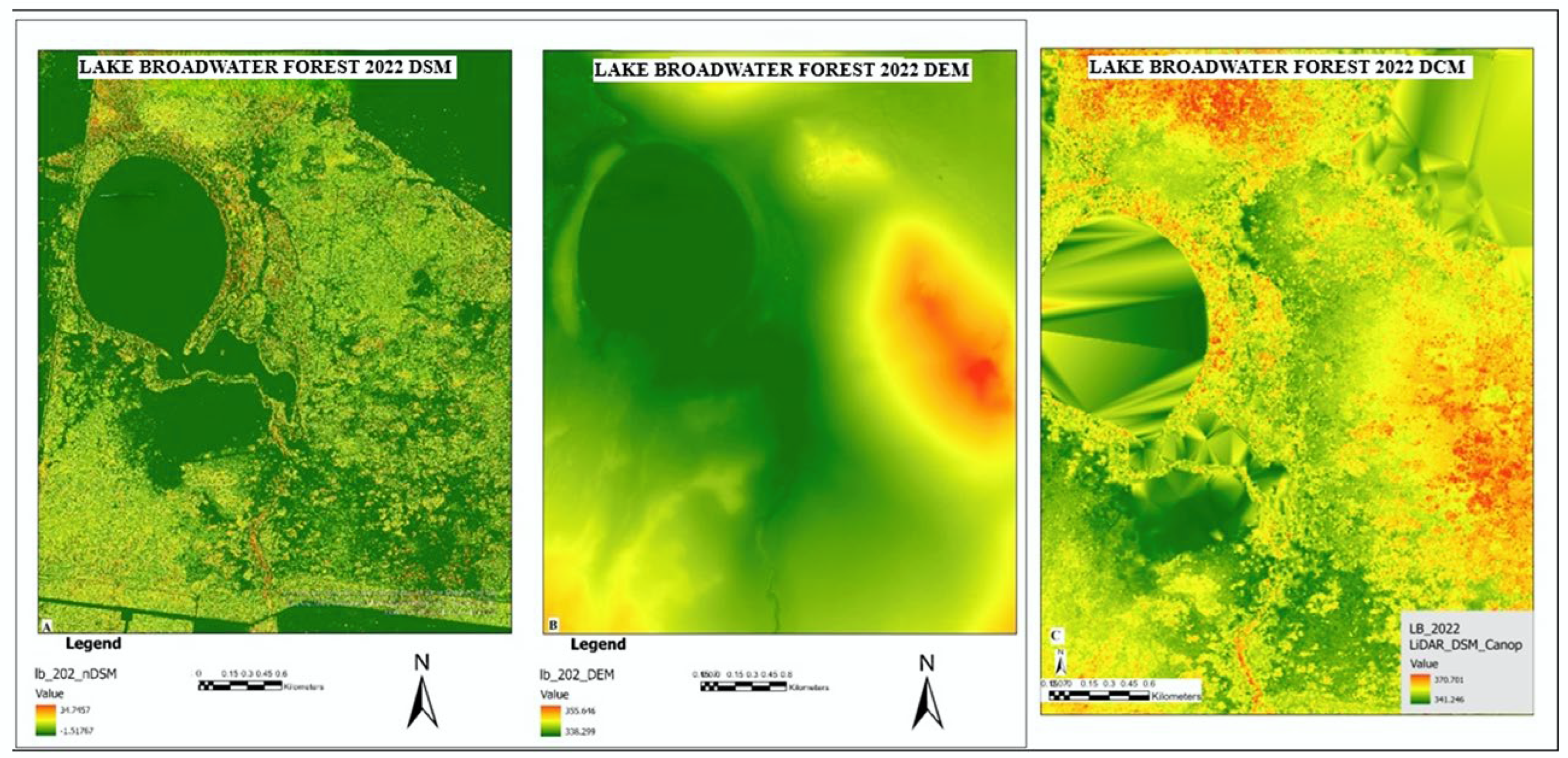
3.1. LiDAR Data Outputs

This section describes 2022 LiDAR forest and tree parameters and the LiDAR data analysis.

3.1.1. LiDAR Data Analysis

The field-visited plots of point-cloud LiDAR data were superimposed over the satellite imagery of the study area, as shown in Figure 4. It can be noted from the relationship between the point cloud data and the satellite imagery that not all trees were detected due to the dense interlocking tree canopy. Point cloud gaps over satellite imagery tree canopies are evident in Plots 7 and 22, which have dense forest canopies. The number of trees that LiDAR data picked up, shown as green triangles in Figure 4, is less than the number of trees on the ground in the visited plots. During the field data collection visit on the ground, there were instances where two or three trees occurred as a cluster with coalesced canopies. However, these were picked up by LiDAR as one tree, which is an underestimation of the tree count by the LiDAR processing algorithm.
The 2012 LiDAR data, which had a very low resolution due to the data collection spacing, underestimated tree height and other tree parameters, caused by incomplete pulse coverage of the scanned area, flaws in the algorithms used to generate the CSM and DTM, and issues related to the pulse’s ability to penetrate the canopy. In the field, the unstable GPS satellite connections and the dense tree canopy cover made it difficult to obtain accurate GNSS readings for locating specific trees within the plots. These issues were resolved by using a compass and tape measure to measure direction and distance from the plot center or another reference point with high positional certainty. Although GNSS survey provides reliable positional information irrespective of weather at all times and anywhere on Earth, it requires an unobstructed line of sight to at least four GNSS satellites for better accuracy. In dense forest, canopy obstruction can significantly degrade signal quality and positional accuracy.
The 2022 LiDAR point cloud was processed in ArcGIS 2.3.0 Pro to generate DEM (Figure 5A) and DSM (Figure 5B) raster images, which were subtracted from each other to develop a DCM (Figure 5C). The DEM shows a high-elevation NW-SE trending ridge with an elevation of 356 m east of the lake. The lowest elevations are the riparian areas of the north-flowing stream and the southeast-flowing stream, which feed into the lake. The lowest elevation is the lake, which has an elevation of 338 m.

3.1.2. 2022 LiDAR Forest and Tree Parameters

The average number of trees per plot is 65, and per hectare is 517. Plots dominated by white cypress pine have more trees than those dominated by brigalow and eucalyptus. This is because white pine trees have apical canopies, and they invest more in height and less in canopy width and volume, resulting in higher stand density. Brigalow and eucalyptus species tend to prioritize canopy development, resulting in fewer trees per plot due to competition for light and other resources. Brigalow and eucalyptus have slightly taller trees than white cypress pine. The average canopy measurements, CD, CA, and CV, are higher in brigalow and eucalyptus trees than in white cypress pine trees with apical canopies. Tree H (m) and measured DBH (cm) were cut off at 5 m and 5 cm, respectively. Canopy diameter, area, and volume had no cut-off, and some values as low as 0.1 m were modeled. The LiDAR-calculated 2022 DBH average underestimated DBH by between 4 and 10 cm, with values ranging from a minimum of 1.2 cm to a maximum of 61.5 cm. The tree plots had average standard deviations of 10 cm and less for 2024-measured DBH and LiDAR 2022 calculated DBH.

3.2. DBH Calculation Models

The average results of the three DBH models (Jucker, Gonzalez-Benecke model 1, and Gonzalez-Benecke 2) were compared against their respective field validation data and are shown in Table 2. All three models underestimated the DBH for all the validation plots. For the 2022 LiDAR data, the Jucker model had the best performance, followed by the Gonzalez-Benecke model 2 and Gonzalez-Benecke model 1 models. The average DBH of the visited plots in the 2022 LiDAR data was 22 cm, while the Jucker, Gonzalez-Benecke model 1, and Gonzalez-Benecke model 2 models had DBHs of 16, 13, and 15 cm, respectively.
Also shown in Table 2, the residuals are the model-calculated values subtracted from the field-measured or observed measurements. On average, the Jucker model had smaller residuals than the Gonzalez-Benecke model 1 and 2, except for Plots 4 and 15, which were dominated by white cypress species, and 24, which brigalow dominated. The other plots are predominantly mixed with white cypress, eucalyptus, and brigalow, and the Jucker model estimated DBH values to be close to the measured values. The rest of the plots have lower single-figure residuals for the Jucker model, followed by Gonzalez-Benecke model 2 with slightly higher figures, and the highest residuals are from Gonzalez-Benecke model 1. Plots 4, 5, and 22 had the highest, and Plots 7, 11, and 15 had the most minor residuals for the Jucker model. Gonzalez-Benecke model 1 and Gonzalez-Benecke model 2 had Plots 5, 6, and 22 with the highest residuals and Plots 7, 11, and 15 with the most minor residuals for the 2022 LiDAR data. In summary, the Jucker model with the 2022 LiDAR data had a better estimate of the DBH than the Gonzalez-Benecke models. The Jucker model uses H and CD, the Gonzalez-Benecke model 1 uses H only, and the Gonzalez-Benecke model 2 uses H and CA.

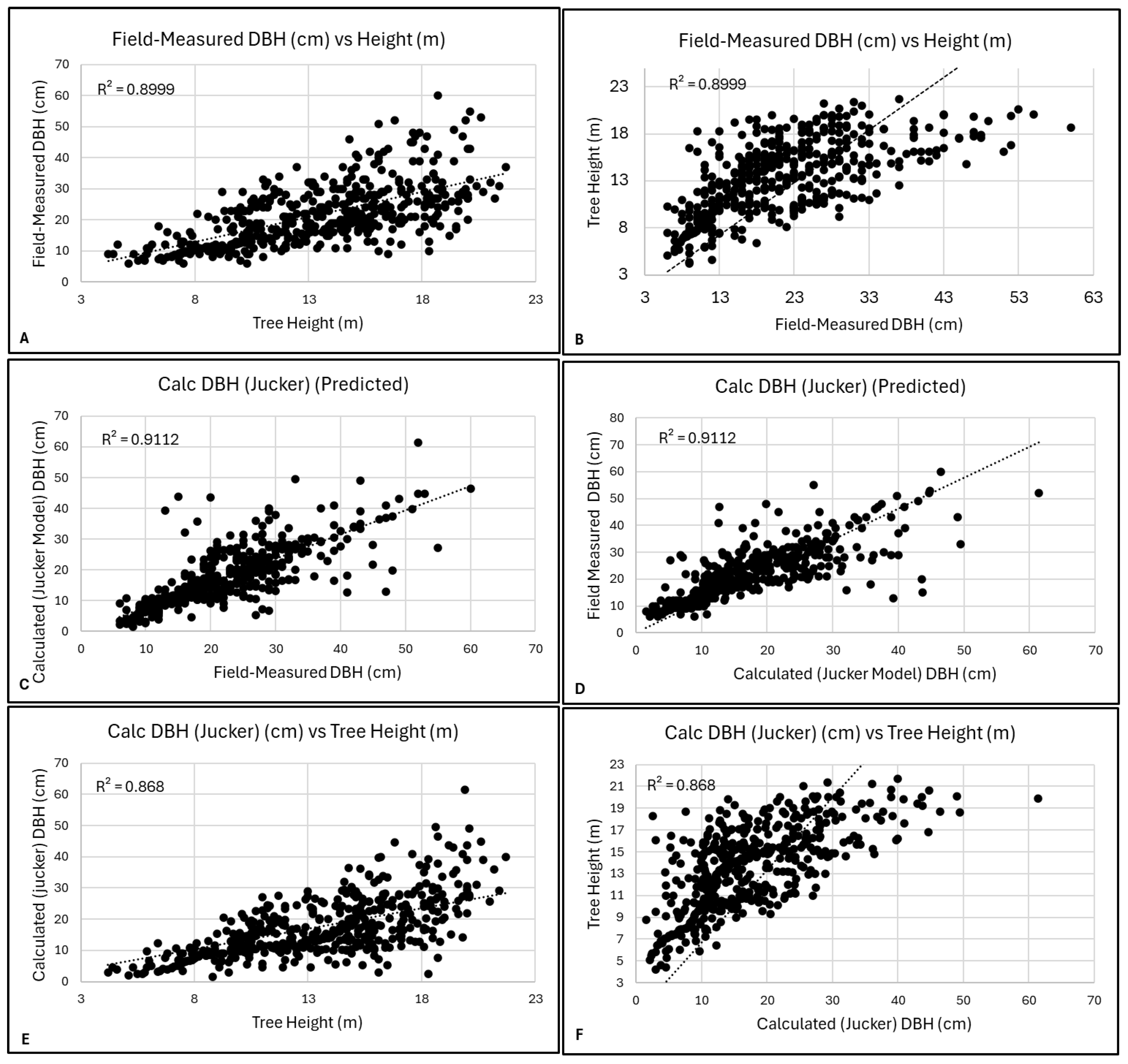
3.2.1. Jucker Model for DBH Calculation

The Jucker model estimates diameter (D) based on height (H) and crown diameter (CD). Figure 6 shows the graphs plotted for different parameters derived from the 2022 LiDAR data and the Jucker Model estimation for DBH. Figure 6A,B show field-measured DBH plotted against tree H, and vice versa, tree H plotted against the field-measured DBH, with an R2 value of 0.9005. Figure 6A shows heteroscedasticity when the field-measured DBH is plotted as a dependent variable against tree H as an independent variable. Figure 6C–E also show the same heteroscedasticity. Figure 6C shows field-measured DBH (cm) plotted as an independent variable versus the Jucker model calculated DBH, and 6D shows the reverse, where the Jucker model DBH is plotted as the independent variable of the field-measured DBH. Heteroscedasticity refers to a condition in statistical models, especially in regression analysis, where the variability of the errors (residuals) changes at different levels of the independent variables, rather than remaining constant. Figure 6C,D show an R2 of 0.8929, and 6E and 6F have an R2 value of 0.8618. Figure 6B,F show that tree height reached an asymptote when plotted against field-measured DBH and Jucker model calculated diameter, respectively. The trees reach maximum height in both graphs but continue growing in diameter and possibly other tree parameters, such as CD, CA, and CV.
Plot 6 is the data validation plot, where individual tree DBH was measured and plotted against its calculated DBH. Despite a few data points, the individual graphs are similar to Figure 6 but with higher R2 values depicting more accurate values. Where tree H is plotted against field-measured DBH, the data shows a high R2 value of 0.9356, higher than the All Plots R2 value of 0.9005. R2 values also increased to 0.8943 from 0.8929 for All Plots. Similarly, the R2 value increased to 0.8696 compared to a value of 0.8618, where tree H was plotted against the calculated Jucker model DBH as a dependent variable and vice versa as an independent variable.

3.2.2. Gonzalez-Benecke Equation (1) Model for DBH Calculation

The Gonzalez-Benecke model 1 estimates diameter using tree H. Figure 7 shows linear graphs with model-calculated DBH, field-measured DBH, and tree H plotted against each other. Figure 7A,C,E,F show heteroskedasticity. Figure 7A,C have tree height plotted as an independent variable against field-measured DBH (cm) and Gonzalez-Benecke model 1 DBH (cm), respectively. Figure 7E,F have field-measured DBH (cm) and the Gonzalez-Benecke model 1 calculated DBH (cm) plotted against each other as dependent and independent variables. Figure 7B,D show an asymptote where field-measured DBH (cm) and Gonzalez-Benecke model 1 DBH (cm) are plotted as independent variables with height as a dependent variable. The graphs also show R2 values for the linear equation, which will be discussed below. The validation plot from Plot 6, which shows specific DBH (cm) plotted against its specific H, and the Gonzalez-Benecke model 1 calculated DBH (cm) show homoscedastic behavior, which differs from the All Plots data in Figure 7. Heteroscedastic behavior is evident where the tree height and field-measured DBH (cm) are plotted against the field-measured DBH and calculated Gonzalez-Benecke model 1 DBH (cm), respectively. Asymptotic behavior is shown where tree H is plotted against field-measured DBH (cm) as its independent variable.

3.2.3. Gonzalez-Benecke Equation (2) Model for DBH Calculation

Like the linear models of the Jucker model graphs in Figure 6 and the Gonzalez-Benecke model 1 in Figure 8, the Gonzalez-Benecke model 2 graphs have the same trends and behavior. Heteroskedasticity is evident, where tree H is plotted as an independent variable to the Gonzalez-Benecke model 2 calculated DBH and the field-measured DBH. Heteroskedasticity is also observed, where the Gonzalez-Benecke model 2 calculated DBH (cm) is plotted against the field-measured DBH (cm) as independent and dependent variables. Asymptotic behavior is seen where tree H is the dependent variable for the field-measured DBH (cm) and the Gonzalez-Benecke model 2 calculated DBH (cm) independent variables. Due to the low data counts, the trends and behavior of the graphs in the validation plot, Plot 6, are unclear, but subtle trends can be deduced. The Gonzalez-Benecke model 2 calculated DBH plotted against tree H shows a high R2 value of 0.9691. The R2 values for graphs where tree height is plotted against field-measured DBH (cm) and where Gonzalez-Benecke model 2 calculated DBH (cm) and field-measured DBH (cm) are plotted against each other are 0.9356 and 0.9433, respectively.

3.3. Model Validation and Performance

Table 3 presents the statistical parameters used to evaluate and compare the goodness of fit for the three DBH models employed in predicting tree DBH within the study area. RMSE, PBias, MAE, MAPE, and R2 were calculated for the validation data from Plot 6 and all 6 plots, including Plot 6, for the three DBH models. The Jucker model statistical parameters for ‘All Plots’ are higher than or equal to the values for Plot 6. The opposite is true for both Gonzalez-Benecke models 1 and 2, where all statistical parameters for Plot 6 are higher than for ‘All Plots’. The Jucker model shows the same RMSE and MAE for Plot 6 and ‘All Plots’ of 8.6 and 6, respectively. The PBias of Plot 6 was lower at 13.54% than the ‘All Plots’ at 21.94%. The MAPE for ‘All Plots’ was 22.05%, higher than that for Plot 6 at 13.63%.
The RMSE, PBias, MAE, and MAPE values for both Gonzalez-Benecke models 1 and 2 are all higher for the validation plot, Plot 6, than for All Plots. The Gonzalez-Benecke model 1 RMSE for Plot 6 is 13.24, and for All Plots, it is 9.29. It has a PBias of 40.35% for Plot 6 and 26.05% for All Plots. The MAE is 12 for Plot 6 and 6 for All Plots. Finally, the Gonzalez-Benecke model 1 has an MAPE value for Plot 6 of 35.13 and 24.56 for All Plots. The Gonzalez-Benecke model 2 RMSE for Plot 6 is 12.36 and 8.93 for All Plots. The PBias is 33.18% and 24.92% for Plot 6 and All Plots, respectively. A Plot 6 MAE value of 8 and an All Plots value of 6 were calculated. The MAPE for All Plots for Gonzalez-Benecke model 2 is almost like Gonzalez-Benecke model 1, with values of 24.26 and 30.99 for Plot 6.

R2 Values for the Jucker and the Gonzalez-Benecke DBH Models

The R2 values for the three DBH models were calculated automatically from the linear model’s graphs. The linear models were for three parameters derived from the 2022 LiDAR data and field-measured DBH plotted as independent and dependent variables of each other. The linear graphs plotted tree height against field-measured DBH and model-calculated DBH for the Jucker model, Gonzalez-Benecke model 1, and Gonzalez-Benecke model 2. The third linear graph plotted field-measured DBH against calculated DBH for the three models. The Jucker model, which exhibits an R2 value like the Gonzalez-Benecke model 1 model, with a value of 0.9005, and the Gonzalez-Benecke model 2 model, with a lower value of 0.8942, when tree height is plotted against the field-measured DBH. Tree height plotted against the model-calculated DBH shows that the Gonzalez-Benecke model 2 has a higher value of 0.8658 compared to the Jucker model, which has the lowest value of 0.8618, and the Gonzalez-Benecke model 1, which has a middle value of 0.8645. The field-measured DBH plotted against the calculated DBH yields the Jucker model, which provides a higher R2 value of 0.8929, followed by the Gonzalez-Benecke model 2, with a value of 0.8813, and the lowest value of 0.8612 for the Gonzalez-Benecke model 1. Based on the R2 value for tree height plotted against the model-calculated DBH, the Gonzalez-Benecke model 2 performed better than the Jucker model and the Gonzalez-Benecke model 1.

3.4. Aboveground Biomass (AGB)

Table 4 summarizes the tree, plot, and hectare total AGB, total biomass, total C, and total CO2 for the 2022 LiDAR-derived Jucker model DBH used in the Chave AGB model. Despite having lower tree counts per plot, Acacia harpophylla and Eucalyptus tree species had more biomass and CO2 sequestered from the atmosphere than the white cypress pine species. Table 4 shows the 2022 LiDAR data-derived biomass average of 180.9 tons/ha against the 2024 total biomass of 249 tons/ha. A total biomass of 249 tons/ha is reasonable and in line with the published literature of the Brigalow region. The Lake Broadwater Forest sequestered an average of 240.7 tons/ha of CO2 in 2022 and 331.3 tons/ha.
The average total biomass and CO2 sequestered by the forest in 2024 are higher than the 2022 LiDAR-derived biomass and CO2. The 2022 LiDAR-derived estimations are lower than the 2024 field-measured estimations because the DBH estimation model underestimated the values, and more biomass could have been added in the one and a half years from 2022 to 2024. However, this difference could also be due to error propagation from LiDAR-based canopy metrics or species-specific misrepresentation in the allometric models.

4. Discussion

4.1. LiDAR Data and Technology

Advancements in LiDAR sensor technology and computational methods now allow for the accurate identification and measurement of individual tree crown dimensions for the first time, representing a significant transformation in forest census methods [60,61]. LiDAR data is now widely available for free from various repositories, and processing is becoming easier and more accessible, although some software remains quite expensive to acquire. Data resolution has also greatly improved to a millimeter scale, with more tree attributes and measured dimensions [22]. The technology changes span hardware design, software capabilities, applications, and integration into various industries. LiDAR data gives tree parameters such as height and canopy dimensions such as diameter, area, and volume. However, they cannot give trunk DBH, an essential parameter in the equations for calculating aboveground biomass (AGB). The DBH calculated from the DBH models can be used in ABG equations where the remotely sensed LiDAR data is collected and processed to give tree height (H) and canopy dimensions. Allometric equations calculate DBH with the tree parameters derived from LiDAR data. The best-performing equation from the 2022 LiDAR data was the Jucker model based on the validation statistics. All three equations underestimated the DBH. The Jucker model gave values close to the field-measured values for the 2022 LiDAR data. The DBH derived from the 2022 LiDAR was compared to the 2024 field-measured DBH, a difference of two years, which could have contributed to the cause of the difference. The field measuring errors with a tape measure and graduated angle ruler, and the subsequent 2-year growth in the tree trunks, could account for the differences in the DBH measurements between the 2022 LiDAR-derived DBH and the 2024 measured DBH. The error could have been reduced by field-measuring the DBH in the same year as the LiDAR data was collected. The error caused by not measuring DBH the same year as LiDAR data collection is negligible over the one and a half years because the tree species under study have a diameter growth of less than 0.5 cm per year [62].

4.2. DBH Estimation Models’ Statistical Metrics

In choosing the best-performing equation, the three DBH models, Jucker, Gonzalez-Benecke model 1, and Gonzalez-Benecke model 2, had their mean absolute percentage error (MAPE), mean absolute error (MAE), percentage bias (PBIAS), root mean square error (RMSE), and R2 calculated and compared for the validation plot (Plot 6) and All Plots put together. For comparison purposes, all the values for the validation parameters were treated as percentage values except for R2, which was discussed separately, and the results are shown in Figure 8. The Jucker model was the best-performing model, followed by the Gonzalez-Benecke model 2 and then the Gonzalez-Benecke model 1. Although useful, these statistical metrics share a common limitation: since their values range from zero to positive infinity, a single value alone provides limited insight into the regression’s performance relative to the distribution of the ground truth data.
Plot 6 had higher values of the compared metrics than All Plots’ values, which is due to population size. Plot 6 had a smaller population than the combined population of all plots. For model comparison, a bigger population would still have given the same overall results and conclusions on the best model.

4.2.1. RMSE and MAE

Several researchers have recommended using MAE instead of RMSE, arguing that RMSE may not be a reliable indicator of average model performance and can misrepresent the average error. Some authors recommend using a combination of metrics, including both RMSE and MAE, to evaluate model performance. RMSE and MAE are not independent, so it can be difficult to weigh their importance in model evaluation [63]. The logical approach is to weigh them by their likelihood. According to the law of likelihoods, the evidence supporting one hypothesis over another is represented by the ratio of their likelihoods [64].

4.2.2. Mean Percentage Bias (MBias)

The Jucker model has lower MBias values for Plot 6 and All Plots than the Gonzalez-Benecke model 1 and Gonzalez-Benecke model 2 models. All three models have negative MBias values, which shows that they all underestimate DBH, with the two Gonzalez-Benecke models underestimating DBH to a greater extent than the Jucker model. Like other metrics used for model performance validation, the Jucker model, which has lower MBIAS, is better. Though the Jucker model has lower values for Plot 6 and All Plots of 13.54% and 21.94%, the values also show that the model is not so good at estimating the DBH. The difference in the observed and the model calculated values could have been caused by errors in measuring the observed values in the field and the 1.5-year difference in the 2022 LiDAR data collection and the measuring of the field observed values in 2024.

4.2.3. Mean Absolute Percentage Error (MAPE)

MAPE is a commonly used metric in regression analysis to assess the accuracy of forecasts or predictions. It expresses the error as a percentage, making interpreting across different datasets or models easier [65,66]. It ignores whether predictions are too high or too low, focusing only on the error size [67]. Thus, MAPE should be applied cautiously when actual values approach zero or in datasets with many outliers [68]. In this research project, the Jucker model again outperformed the Gonzalez-Benecke model 1 and Gonzalez-Benecke model 2 models, especially in the Plot 6 results, where the Jucker model was less than half the value of the Gonzalez-Benecke models, with a value of 13.63, and the Gonzalez-Benecke model had values of 35.13 and 30.99, respectively. The Plot 6 Jucker model values are closer to observed values or have a smaller absolute error, followed by Gonzalez-Benecke model 2 and Gonzalez-Benecke model 1 as the least performers.

4.2.4. Coefficient of Determination (R2)

The coefficient of determination (R2) suggests the model’s goodness of fit, meaning how well the regression model’s predicted values match the actual data. Tree H was plotted against field-measured DBH, and the calculated DBH for Plot 6 had the Gonzalez-Benecke model 2 with the highest values, followed by Gonzalez-Benecke model 1 and the Jucker model with the smallest values. Therefore, the Gonzalez-Benecke model 2 is a better model, as indicated by the coefficient of determination. The All Plots results were the reverse of Plot 6, where tree H was plotted against field-measured values using the Jucker model and Gonzalez-Benecke model 1, with higher values of 0.9005 compared to Gonzalez-Benecke model 2, which had a value of 0.8942. All Plots tree H plotted against calculated DBH had the lowest R2 values of 0.8618, 0.8645, and 0.8658 for Jucker, Gonzalez-Benecke model 1, and Gonzalez-Benecke model 2 models, respectively. A high R-squared value does not always indicate that the model is reliable or well fitted. It only measures the degree of variability the model explains, not the accuracy of individual predictions [66]. The drawback of R2 is that it does not indicate the accuracy of predictions but only reflects the proportion of explained variance and does not account for model complexity or the significance of predictors [69,70]. Another limitation is that R2 increases with the addition of more predictors, even if those predictors are not statistically significant. R2 will increase when more variables are added to the model [71]. Adjusted R-squared is often used to penalize models for including unnecessary predictors that do not enhance the model’s fit.

4.2.5. DBH Models’ Performance

From the above statistical metrics, the Jucker model has come out as the best performance model to estimate DBH, though it also underestimated DBH. The Jucker model used a compound variable of the effect of H and CD (as opposed to separately including the two predictors in the model) to avoid issues with collinearity resulting from the non-independence of H and CD [72]. Combined H and CD proved to be a better predictor of D than a model with H and CD as separate explanatory variables [39]. The Gonzalez-Benecke model 1 included H only, and the Gonzalez-Benecke model 2 included H and CA, which is why the Gonzalez-Benecke model 2 performed better than the Gonzalez-Benecke model 1. Other research studies have found that estimating stem diameter requires considering both H and crown size, with crown size being crucial for distinguishing between trees of similar height but significantly different trunk diameters [73,74]. Lake Broadwater Forest is a mixed tree species forest with trees of various sizes in height and canopy dimensions. This implies that an allometric equation excluding height and canopy dimensions would likely underestimate D and AGB. Trees with smaller diameters dominate most forests; therefore, any regression analysis signal will be biased, as observed in this research project. The best way to address this issue is by using binned data instead of raw data [75]. This project did not implement the data binning method because it reduces tree-level variation in allometric attributes to a mean value [76]. However, a major drawback of this approach is that it inevitably underestimates the true uncertainty of the model. Allometric relationships between D, H, CD, and CA are strongly influenced by climate, geographic regions, species type, and soil conditions [77,78].
Lake Broadwater Forest comprises different tree species with different tree growth habits, soil type requirements, and moisture needs. These requirements give the variation in the forest trees that is seen in the Brigalow Belt of Queensland and northern New South Wales, which covers the Lake Broadwater Forest. The study plots were selected based on the vegetation type, density, soil type (geology), and elevation. Many vegetation communities within the Brigalow Belt are defined by the presence of brigalow (Acacia harpophylla), a leguminous tree typically reaching heights of 12–15 m and commonly occurring in open forests and woodlands [79]. The fertile cracking clay soils (vertosols) that support brigalow communities have made them prime targets for extensive clearing to accommodate agricultural and pastoral activities [80,81]. The remaining brigalow forests are now classified as endangered ecological communities under Australia’s Environment Protection and Biodiversity Conservation Act 1999 and as endangered regional ecosystems under the Queensland Vegetation Management Act 1999 [82,83,84].
Within the Lake Broadwater Forest, two main tree functional groups should be considered to improve the accuracy of the predictive models. These include angiosperms (brigalow and eucalyptus) and gymnosperms (white cypress pine), which exhibit different tree heights and canopy growth patterns. The contrasting crown architecture of these two groups—gymnosperms generally exhibit strong apical dominance and invest heavily in height growth, whereas angiosperm trees possess a greater ability to support the structural growth of trees—will determine whether they will invest in height or canopy development [85,86].

4.2.6. Graphical Interpretations (Asymptote and Heteroskedasticity)

The results graphs in Section 4 show asymptotic and heteroskedasticity behaviors. The asymptotic behavior is seen when tree height is plotted against calculated and field-measured DBH. The trees continue to grow in stem thickness or DBH, and their height increases at a diminishing rate, approaching a biological and structural limit. Young trees primarily allocate resources to height growth to escape shaded understories, quickly reaching their maximum height while continuing to increase in diameter throughout their lifespan [73]. This makes estimating the diameter of large trees challenging since trees of similar height can have significantly different diameters. This poses a problem for biomass estimations, leading to underestimating total AGB in forests by 10–30% in forests with large individuals, as large-diameter trees store the majority of the biomass [87,88,89]. In this context, crown size information may be crucial for accurately estimating a tree’s diameter [39]. While height growth in large trees slows quickly, lateral crown expansion continues, necessitating ongoing investment in stem growth to maintain structural stability and hydraulic function [74,90]. Power-law models or their log-transformed linear equivalents allow for continuous scaling across a broad DBH spectrum without imposing artificial upper limits [91].
Heteroscedasticity, characterized by increasing residual variance with increasing predictor magnitude, is a common phenomenon in allometric models used for forest structural assessments [92,93]. In models where biomass or height is predicted from diameter at breast height (DBH), larger trees tend to exhibit greater variability in form, crown shape, and taper, resulting in non-constant error variance as evidenced in Figure 6 and Figure 7. While ordinary least squares (OLS) regression remains unbiased under heteroscedasticity, it yields inefficient estimates with unreliable standard errors and confidence intervals, particularly at the upper DBH range [75]. To correct for this, the log-transformation of both dependent and independent variables is often employed to stabilize variance across DBH classes. Additionally, weighted least squares (WLS) can assign smaller weights to high-variance observations, thereby improving model efficiency [20], while generalized least squares (GLS) and linear mixed-effects models can explicitly model heteroscedastic variance structures or account for nested sources of variation such as site or species effects [94].

4.3. ABG and Carbon Sequestration

The results of the 2022 Lidar-derived AGB and the 2024 field-measured DBH were in the expected AGB estimation range of the Brigalow region of SE Queensland in Australia. The C and CO2 sequestered by the Lake Broadwater Forest included BGB but excluded dead wood, soil, and undergrowth biomass, which means there was an underestimation of the total biomass and, ultimately, the C and CO2. The role of forest ecosystems in conserving and enhancing carbon (C) sinks has been widely recognized, as they play a crucial part in mitigating climate change by absorbing and storing carbon, thus helping to reduce global warming [95,96,97,98,99,100]. Forests function as mechanisms for capturing additional carbon and serve as carbon reservoirs across various carbon pools, including aboveground, root, and litter [101,102]. Accurate forest biomass estimation is crucial, as it provides valuable data on ecosystem productivity, nutrient flows, and the role of forests in the global carbon cycle [97,103]. Therefore, quantifying terrestrial forest AGB is essential for various global initiatives, such as REDD+, which supports Payment for Ecosystem Services (PES), as well as for accounting, monitoring, and developing strategies for the sustainable management of forests.
Landholders are essential stakeholders in any country’s carbon emissions mitigation programs, as they own vast amounts of forests. They need to be encouraged to participate in carbon farming and be recognized for their efforts in reducing carbon emissions. By participating in a carbon credit system, farmers can earn credits for reducing emissions. These credits can then be sold on a carbon credit market to emitters who need to purchase offsets to comply with their mandated emission limits [104]. In Australia, carbon calculations for carbon credits are part of the Emissions Reduction Fund (ERF), now managed under the Climate Solutions Fund (CSF) [105,106]. This government-led program incentivizes projects that reduce greenhouse gas emissions or sequester carbon through land management, reforestation, agriculture, energy efficiency, and other methods [107,108]. Through enhanced agricultural land-management practices, foresters, ranchers, and farmers can boost the transfer of carbon from the air into the soil. As a result, agricultural carbon credits from increased carbon sequestration are anticipated to play a key role in reaching carbon-neutrality targets [109,110].

5. Conclusions

Further research is needed to derive DBH or stem diameter from LiDAR data, as current technology does not yet support the direct extraction of this important parameter used in AGB allometric equations. Several global pantropical and regional allometric equations and models have been developed to calculate DBH, and a selection must be made regarding which one to use. The models used in this study are the global pantropical models developed by Jucker and Gonzalez-Benecke, which can be applied anywhere in the world. Developing specific allometric equations for the Brigalow region is necessary, as we do not have any models to use. The main issue with the models used in this study was the heteroskedasticity displayed by the regression equations and graphs that used H as an independent variable. This was caused by the fact that when trees reach their maximum H, they will invest in crown dimensions and stem thickness, increasing the dependent variable’s error variation.
The Jucker model proved to be better than the Gonzalez-Benecke model 1 and 2 models in estimating DBH, as proved by the performance or validation metrics used, such as RMSE, MAE, MAPE, PBias, and R2. The five performance metrics used in this study all showed that the Jucker model had better performance, indicating no need to use all available metrics. Two or three metrics will suffice. These metrics are vital in regression analysis, machine learning, and statistical modeling, allowing comparison across models and helping to select the most accurate one. Though the Jucker model had better performance, it underestimated DBH, but it proved that it could be used. The Chave AGB model was used to calculate AGB using the DBH estimated by the Jucker model, and this was compared with AGB estimated using the field-measured DBH. It has been demonstrated that different tree species have different capacities to process carbon into biomass due to their tree species characteristics. A key factor in this study was the difference between angiosperms and gymnosperms, which resulted in significantly different AGB values. The angiosperms, eucalyptus, and brigalow had lower tree stand densities, and the gymnosperms, represented predominantly by white cypress pine, had high tree stand densities but lower values of AGB per hectare. It is important to know which forest type should be promoted in the region for carbon farming and sequestration efficiencies. The research proved that the eucalyptus and brigalow forests should be promoted ahead of white cypress pine forests. The landholders (farmers) and mining companies can develop and manage the eucalyptus and brigalow forests to reduce their carbon footprint, reduce their carbon tax budgets, and direct the resources to their operations. The involvement of landholders is critical in the greenhouse gas reduction programs for the country to meet its climate change targets. It was also evident that as trees mature, their capacity to sequester carbon increases, making older trees more effective at absorbing CO2. This relationship highlights the significance of forest conservation and the critical role mature trees play in mitigating climate change. By understanding and supporting these natural processes, we can enhance the capacity of forests to function as carbon sinks, thereby contributing to global efforts to balance our planet’s carbon cycle and tackle the growing challenges of climate change.

Author Contributions

Conceptualization, Z.M.B., X.L., Z.Z. and D.R.P.; methodology, Z.M.B., X.L., Z.Z. and D.R.P.; software, Z.M.B. and X.L.; writing—original draft, Z.M.B.; writing—review and editing, X.L., Z.Z. and D.R.P.; supervision, X.L., Z.Z. and D.R.P.; project administration, X.L. All authors have read and agreed to the published version of the manuscript.

Funding

This research received no external funding.

Data Availability Statement

The raw data supporting the conclusions of this article will be made available by the authors on request.

Acknowledgments

All data collected in the field and used in this project will be made available on request. LiDAR point cloud data was obtained from: https://elevation.fsdf.org.au/ (accessed on 12 June 2024).

Conflicts of Interest

The authors declare that they have no known competing financial interests or personal relationships that could have appeared to influence the work in this paper.

Abbreviations

AGBAbove-Ground Biomass
AGCAbove-ground Carbon
AHDAustralian Height Datum
ALSAirborne Laser Scanning
AvAverage
BGBBelow Ground Biomass
CCarbon
CACanopy Area
CDCanopy Diameter
CD N_SCanopy Diameter North_South
CD E_WCanopy Diameter East_West
CHCanopy Height
CO2Carbon Dioxide
CVCanopy Volume
DDiameter
DBHDiameter at Breast Height
DCMDigital Canopy Model
DEMDigital Elevation Model
DETSIDepartment of Environment, Tourism, Science and Innovation
DSMDigital Surface Model
nDSMNormalized Digital Surface Model
ELVISEarth Observation and Land-Vectoring Infrastructure System
EuEucalyptus
GDAGeocentric Datum of Australia
GISGeographical Information System
GNSSGlobal Navigation Satellite System
HaHectare
HAGLHeight Above Ground Level
IPCCIntergovernmental Panel on Climate Change
LASLiDAR Aerial Survey
LiDARLight Detection and Ranging
MBiasMean Percentage Bias
MAEMean Absolute Error
MAPEMean Absolute Percentage Error
MgMega Gram
R2Coefficient of Determination
RMSERoot Mean Square Error
SOCSoil Organic Carbon
TPHTrees per Hectare

References

  1. Xu, D.; Wang, H.; Xu, W.; Luan, Z.; Xu, X. LiDAR applications to estimate forest biomass at individual tree scale: Opportunities, challenges and future perspectives. Forests 2021, 12, 550. [Google Scholar] [CrossRef]
  2. Lu, D.; Chen, Q.; Wang, G.; Liu, L.; Li, G.; Moran, E. A survey of remote sensing-based aboveground biomass estimation methods in forest ecosystems. Int. J. Digit. Earth 2016, 9, 63–105. [Google Scholar] [CrossRef]
  3. Riano, D.; Chuvieco, E.; Condés, S.; González-Matesanz, J.; Ustin, S.L. Generation of crown bulk density for Pinus sylvestris L. from lidar. Remote Sens. Environ. 2004, 92, 345–352. [Google Scholar] [CrossRef]
  4. Fauzi, N.; Hambali, K.; Nawawi, S.; Busu, I.; Yew, S. Biomass and carbon stock estimation along different altitudinal gradients in tropical forest of Gunung Basor, Kelantan, Malaysia. Malay. Nat. J. 2017, 69, 57–62. [Google Scholar]
  5. Gubena, A.F.; Soromessa, T. Variations in forest carbon stocks along environmental gradients in egdu forest of oromia region, ethiopia: Implications for sustainable forest management. Am. J. Environ. Prot. 2016, 12, 1–8. [Google Scholar]
  6. Joshi, R.; Singh, H. Carbon sequestration potential of disturbed and non-disturbed forest ecosystem: A tool for mitigating climate change. Afr. J. Environ. Sci. Technol. 2020, 14, 385–393. [Google Scholar] [CrossRef]
  7. Fawzy, S.; Osman, A.I.; Doran, J.; Rooney, D.W. Strategies for mitigation of climate change: A review. Environ. Chem. Lett. 2020, 18, 2069–2094. [Google Scholar] [CrossRef]
  8. McRoberts, R.E.; Næsset, E.; Gobakken, T.; Bollandsås, O.M. Indirect and direct estimation of forest biomass change using forest inventory and airborne laser scanning data. Remote Sens. Environ. 2015, 164, 36–42. [Google Scholar] [CrossRef]
  9. Gonzalez-Benecke, C.; Gezan, S.A.; Samuelson, L.J.; Cropper, W.P.; Leduc, D.J.; Martin, T.A. Estimating Pinus palustris tree diameter and stem volume from tree height, crown area and stand-level parameters. J. For. Res. 2014, 25, 43–52. [Google Scholar] [CrossRef]
  10. West, P. Biomass. In Tree and Forest Measurement; Springer: Berlin/Heidelberg, Germany, 2015; pp. 53–70. [Google Scholar]
  11. Torre-Tojal, L.; Bastarrika, A.; Boyano, A.; Lopez-Guede, J.M.; Grana, M. Above-ground biomass estimation from LiDAR data using random forest algorithms. J. Comput. Sci. 2022, 58, 101517. [Google Scholar] [CrossRef]
  12. Fonseka, C. Extracting dendrometric parameters of urban trees using remotely sensed data for quantifying their ecological services in Valls Hage. Master’s Thesis, University of Gävle, Gävle, Sweden, 2023. [Google Scholar]
  13. Walker, S.M.; Murray, L.; Tepe, T. Allometric Equation Evaluation Guidance Document; Winrock International: Little Rock, AR, USA, 2016. [Google Scholar]
  14. Galán, C.O.; Rodríguez-Pérez, J.R.; Torres, J.M.; Nieto, P.G. Analysis of the influence of forest environments on the accuracy of GPS measurements by using genetic algorithms. Math. Comput. Model. 2011, 54, 1829–1834. [Google Scholar] [CrossRef]
  15. Mukuralinda, A.; Kuyah, S.; Ruzibiza, M.; Ndoli, A.; Nabahungu, N.L.; Muthuri, C. Allometric equations, wood density and partitioning of aboveground biomass in the arboretum of Ruhande, Rwanda. Trees For. People 2021, 3, 100050. [Google Scholar] [CrossRef]
  16. Khan, M.N.I.; Islam, M.R.; Rahman, A.; Azad, M.S.; Mollick, A.S.; Kamruzzaman, M.; Sadath, M.N.; Feroz, S.; Rakkibu, M.G.; Knohl, A. Allometric relationships of stand level carbon stocks to basal area, tree height and wood density of nine tree species in Bangladesh. Glob. Ecol. Conserv. 2020, 22, e01025. [Google Scholar] [CrossRef]
  17. Delcourt, C.J.F.; Veraverbeke, S. Allometric equations and wood density parameters for estimating aboveground and woody debris biomass in Cajander larch (Larix cajanderi) forests of northeast Siberia. Biogeosciences 2022, 19, 4499–4520. [Google Scholar] [CrossRef]
  18. Torgersen, C.E.; Le Pichon, C.; Fullerton, A.H.; Dugdale, S.J.; Duda, J.J.; Giovannini, F.; Tales, É.; Belliard, J.; Branco, P.; Bergeron, N.E.; et al. Riverscape approaches in practice: Perspectives and applications. Biol. Rev. 2022, 97, 481–504. [Google Scholar] [CrossRef] [PubMed]
  19. Ferraz, A.; Saatchi, S.; Mallet, C.; Meyer, V. Lidar detection of individual tree size in tropical forests. Remote Sens. Environ. 2016, 183, 318–333. [Google Scholar] [CrossRef]
  20. Gonzalez de Tanago, J.; Lau, A.; Bartholomeus, H.; Herold, M.; Avitabile, V.; Raumonen, P.; Martius, C.; Goodman, R.C.; Disney, M.; Manuri, S.; et al. Estimation of above-ground biomass of large tropical trees with terrestrial LiDAR. Methods Ecol. Evol. 2018, 9, 223–234. [Google Scholar] [CrossRef]
  21. Caccamo, G.; Iqbal, I.; Osborn, J.; Bi, H.; Arkley, K.; Melville, G.; Aurik, D.; Stone, C. Comparing yield estimates derived from LiDAR and aerial photogrammetric point-cloud data with cut-to-length harvester data in a Pinus radiata plantation in Tasmania. Aust. For. 2018, 81, 131–141. [Google Scholar] [CrossRef]
  22. Pu, R. Mapping tree species using advanced remote sensing technologies: A state-of-the-art review and perspective. J. Remote Sens. 2021, 2021, 9812624. [Google Scholar] [CrossRef]
  23. Yermo, M.; Laso, R.; Lorenzo, O.G.; Pena, T.F.; Cabaleiro, J.C.; Rivera, F.F.; Vilariño, D.L. Powerline detection and characterization in general-purpose airborne LiDAR surveys. IEEE J. Sel. Top. Appl. Earth Obs. Remote Sens. 2024, 17, 10137–10157. [Google Scholar] [CrossRef]
  24. Terryn, L.; Calders, K.; Bartholomeus, H.; Bartolo, R.E.; Brede, B.; D’hont, B.; Disney, M.; Herold, M.; Lau, A.; Shenkin, A.; et al. Quantifying tropical forest structure through terrestrial and UAV laser scanning fusion in Australian rainforests. Remote Sens. Environ. 2022, 271, 112912. [Google Scholar] [CrossRef]
  25. Baccini, A.; Goetz, S.; Walker, W.; Laporte, N.; Sun, M.; Sulla-Menashe, D.; Hackler, J.; Beck, P.; Dubayah, R.; Friedl, M.; et al. Estimated carbon dioxide emissions from tropical deforestation improved by carbon-density maps. Nat. Clim. Change 2012, 2, 182–185. [Google Scholar] [CrossRef]
  26. Avitabile, V.; Herold, M.; Heuvelink, G.B.; Lewis, S.L.; Phillips, O.L.; Asner, G.P.; Armston, J.; Ashton, P.S.; Banin, L.; Bayol, N.; et al. An integrated pan-tropical biomass map using multiple reference datasets. Glob. Change Biol. 2016, 22, 1406–1420. [Google Scholar] [CrossRef] [PubMed]
  27. Xiao, J.; Chevallier, F.; Gomez, C.; Guanter, L.; Hicke, J.A.; Huete, A.R.; Ichii, K.; Ni, W.; Pang, Y.; Rahman, A.F.; et al. Remote sensing of the terrestrial carbon cycle: A review of advances over 50 years. Remote Sens. Environ. 2019, 233, 111383. [Google Scholar] [CrossRef]
  28. Santoro, M.; Cartus, O.; Carvalhais, N.; Rozendaal, D.M.; Avitabile, V.; Araza, A.; De Bruin, S.; Herold, M.; Quegan, S.; Rodríguez-Veiga, P.; et al. The global forest above-ground biomass pool for 2010 estimated from high-resolution satellite observations. Earth Syst. Sci. Data 2021, 13, 3927–3950. [Google Scholar] [CrossRef]
  29. Jurjević, L.; Liang, X.; Gašparović, M.; Balenović, I. Is field-measured tree height as reliable as believed–Part II, A comparison study of tree height estimates from conventional field measurement and low-cost close-range remote sensing in a deciduous forest. ISPRS J. Photogramm. Remote Sens. 2020, 169, 227–241. [Google Scholar] [CrossRef]
  30. Liao, K.; Li, Y.; Zou, B.; Li, D.; Lu, D. Examining the role of UAV Lidar data in improving tree volume calculation accuracy. Remote Sens. 2022, 14, 4410. [Google Scholar] [CrossRef]
  31. Shao, T.; Qu, Y.; Du, J. A low-cost integrated sensor for measuring tree diameter at breast height (DBH). Comput. Electron. Agric. 2022, 199, 107140. [Google Scholar] [CrossRef]
  32. Cao, L.; Gao, S.; Li, P.; Yun, T.; Shen, X.; Ruan, H. Aboveground biomass estimation of individual trees in a coastal planted forest using full-waveform airborne laser scanning data. Remote Sens. 2016, 8, 729. [Google Scholar] [CrossRef]
  33. Cao, A.; Esteban, M.; Onuki, M.; Takagi, H.; Thao, N.D.; Tsuchiya, N. Future of Asian Deltaic Megacities under sea level rise and land subsidence: Current adaptation pathways for Tokyo, Jakarta, Manila, and Ho Chi Minh City. Curr. Opin. Environ. Sustain. 2021, 50, 87–97. [Google Scholar] [CrossRef]
  34. Ahmad, A.; Gilani, H.; Ahmad, S.R. Forest aboveground biomass estimation and mapping through high-resolution optical satellite imagery—A literature review. Forests 2021, 12, 914. [Google Scholar] [CrossRef]
  35. Coops, N.C.; Tompalski, P.; Goodbody, T.R.; Queinnec, M.; Luther, J.E.; Bolton, D.K.; White, J.C.; Wulder, M.A.; van Lier, O.R.; Hermosilla, T. Modelling lidar-derived estimates of forest attributes over space and time: A review of approaches and future trends. Remote Sens. Environ. 2021, 260, 112477. [Google Scholar] [CrossRef]
  36. Willkens, D.S.; Liu, J.; Alathamneh, S. A case study of integrating terrestrial laser scanning (TLS) and building information modeling (BIM) in heritage bridge documentation: The Edmund Pettus Bridge. Buildings 2024, 14, 1940. [Google Scholar] [CrossRef]
  37. Bi, H.; Fox, J.C.; Li, Y.; Lei, Y.; Pang, Y. Evaluation of nonlinear equations for predicting diameter from tree height. Can. J. For. Res. 2012, 42, 789–806. [Google Scholar] [CrossRef]
  38. Gonzalez-Benecke, C.A.; Fernández, M.P.; Gayoso, J.; Pincheira, M.; Wightman, M.G. Using Tree Height, Crown Area and Stand-Level Parameters to Estimate Tree Diameter, Volume, and Biomass of Pinus radiata, Eucalyptus globulus and Eucalyptus nitens. Forests 2022, 13, 2043. [Google Scholar] [CrossRef]
  39. Jucker, T.; Caspersen, J.; Chave, J.; Antin, C.; Barbier, N.; Bongers, F.; Dalponte, M.; van Ewijk, K.Y.; Forrester, D.I.; Haeni, M.; et al. Allometric equations for integrating remote sensing imagery into forest monitoring programmes. Glob. Change Biol. 2017, 23, 177–190. [Google Scholar] [CrossRef] [PubMed]
  40. Department of the Environment, T.; Science and Innovation. Lake Broadwater Tourist Park. 2024. Available online: https://www.desi.qld.gov.au/ (accessed on 26 April 2024).
  41. Howard, M.; Pearl, H.; McDonald, B.; Shimizu, Y.; Srivastava, S.K.; Shapcott, A. The Conservation of Biodiverse and Threatened Dry Rainforest Plant Communities Is Vital in a Changing Climate. Conservation 2024, 4, 657–684. [Google Scholar] [CrossRef]
  42. Collette, J.C.; Emery, N.J. A new project investigating the floral phenology and seed biology of threatened ecological communities in northwest NSW. Australas. Plant Conserv. J. Aust. Netw. Plant Conserv. 2020, 29, 21–25. [Google Scholar] [CrossRef]
  43. Ahmad, F.; Goparaju, L.; Qayum, A. Natural resource mapping using Landsat and LIDAR towards identifying digital elevation, digital surface and canopy height models. Int. J. Environ. Sci. Nat. Res. 2017, 2, 555580. [Google Scholar]
  44. Nam, V.T.; Van Kuijk, M.; Anten, N.P. Allometric equations for aboveground and belowground biomass estimations in an evergreen forest in Vietnam. PLoS ONE 2016, 11, e0156827. [Google Scholar] [CrossRef] [PubMed]
  45. Balenović, I.; Simic Milas, A.; Marjanović, H. A comparison of stand-level volume estimates from image-based canopy height models of different spatial resolutions. Remote Sens. 2017, 9, 205. [Google Scholar] [CrossRef]
  46. Tristan, G. Calculate Vegetation Biomass from LiDAR Data in Python. 2024. Available online: https://www.neonscience.org/resources/learning-hub/tutorials/calc-biomass-py (accessed on 24 July 2024).
  47. Pucha-Cofrep, F.; Fries, A. ArcGIS Pro Manual; Franz Pucha Cofrep: Senftenberg, Germany, 2025; ISBN 9942510400. [Google Scholar]
  48. Baskerville, G. Use of logarithmic regression in the estimation of plant biomass. Can. J. For. Res. 1972, 2, 49–53. [Google Scholar] [CrossRef]
  49. Chave, J.; Andalo, C.; Brown, S.; Cairns, M.A.; Chambers, J.Q.; Eamus, D.; Fölster, H.; Fromard, F.; Higuchi, N.; Kira, T.; et al. Tree allometry and improved estimation of carbon stocks and balance in tropical forests. Oecologia 2005, 145, 87–99. [Google Scholar] [CrossRef] [PubMed]
  50. Dawkins, H. Estimating total volume of some Caribbean trees. Caribb. For. 1961, 22, 62–63. [Google Scholar]
  51. Chave, J.; Réjou-Méchain, M.; Búrquez, A.; Chidumayo, E.; Colgan, M.S.; Delitti, W.B.; Duque, A.; Eid, T.; Fearnside, P.M.; Goodman, R.C.; et al. Improved allometric models to estimate the aboveground biomass of tropical trees. Glob. Change Biol. 2014, 20, 3177–3190. [Google Scholar] [CrossRef] [PubMed]
  52. Ding, L.; Li, Z.; Shen, B.; Wang, X.; Xu, D.; Yan, R.; Yan, Y.; Xin, X.; Xiao, J.; Li, M.; et al. Spatial patterns and driving factors of aboveground and belowground biomass over the eastern Eurasian steppe. Sci. Total Environ. 2022, 803, 149700. [Google Scholar] [CrossRef] [PubMed]
  53. Patel, K.; Shakhela, R.; Jat, J. Growth, biomass production and CO2 sequestration of some important multipurpose trees under rainfed condition. Int. J. Curr. Microbiol. Appl. Sci. 2017, 6, 1943–1950. [Google Scholar] [CrossRef]
  54. Boomiraj, K.; Jagadeeswaran, R.; Karthik, S.; Poornima, R.; Jothimani, S.; Sudhagar, R.J. Assessing the Carbon Sequestration Potential of Coconut Plantation in Vellore District of Tamil Nadu, India. Int. J. Environ. Clim. Change 2020, 10, 618–624. [Google Scholar] [CrossRef]
  55. Khokher, F.K.; Khan, A.U.; Bargali, H.S.; Ahmed, S.; Gobato, R.; Zaman, S.; Mitra, A. Stored carbon in dominant mangrove species in Indian Sundarbans: A situation analysis with two different methods. Parana. J. Sci. Educ. 2023, 9, 1–9. [Google Scholar]
  56. Lawal, A.; Ayeni, O.; Ayanniyi, O. Carbon-dioxide sequestration potential of trees species in Nigerian Tertiary Institutions: A case study of Ondo State, Nigeria. World News Nat. Sci. 2023, 50, 247–257. [Google Scholar]
  57. Dada, A.D.; Matthew, O.J.; Odiwe, A.I. Nexus between carbon stock, biomass, and CO2 emission of woody species composition: Evidence from Ise-Ekiti Forest Reserve, Southwestern Nigeria. Carbon. Res. 2024, 3, 40. [Google Scholar] [CrossRef]
  58. Ahmed, M.; Miah, M.; Abdullah, H.; Hossain, M.; Rubayet, M. Measurement of Sequestered Standing Carbon Stock in Major Agroforestry Tree Species. Can. J. Agric. Crops 2020, 5, 153–159. [Google Scholar]
  59. Konishi, S.; Kitagawa, G. Information Criteria and Statistical Modeling; Springer Science & Business Media: New York, NY, USA, 2008. [Google Scholar]
  60. Li, N.; Ho, C.P.; Xue, J.; Lim, L.W.; Chen, G.; Fu, Y.H.; Lee, L.Y.T. A progress review on solid-state LiDAR and nanophotonics-based LiDAR sensors. Laser Photonics Rev. 2022, 16, 2100511. [Google Scholar] [CrossRef]
  61. Sharma, M.; Garg, R.D.; Badenko, V.; Fedotov, A.; Min, L.; Yao, A. Potential of airborne LiDAR data for terrain parameters extraction. Quat. Int. 2021, 575, 317–327. [Google Scholar] [CrossRef]
  62. West, P. Modelling maximum stem basal area growth rates of individual trees of Eucalyptus pilularis Smith. For. Sci. 2021, 67, 633–636. [Google Scholar] [CrossRef]
  63. Hodson, T.O. Root mean square error (RMSE) or mean absolute error (MAE): When to use them or not. Geosci. Model. Dev. Discuss. 2022, 15, 5481–5487. [Google Scholar] [CrossRef]
  64. Zhang, Z. A law of likelihood for composite hypotheses. arXiv 2009, arXiv:0901.0463. [Google Scholar]
  65. De Myttenaere, A.; Golden, B.; Le Grand, B.; Rossi, F. Mean absolute percentage error for regression models. Neurocomputing 2016, 192, 38–48. [Google Scholar] [CrossRef]
  66. Hyndman, R.; Athanasopoulos, G. Forecasting: Principles and Practice; OTexts: Melbourne, Australia, 2018. [Google Scholar]
  67. Makridakis, S.; Wheelwright, S.C.; Hyndman, R.J. Forecasting Methods and Applications; John Wiley & Sons: Hoboken, NJ, USA, 2008. [Google Scholar]
  68. Tofallis, C. A better measure of relative prediction accuracy for model selection and model estimation. J. Oper. Res. Soc. 2015, 66, 1352–1362. [Google Scholar] [CrossRef]
  69. Burnham, K.P.; Anderson, D.R.; Huyvaert, K.P. AIC model selection and multimodel inference in behavioral ecology: Some background, observations, and comparisons. Behav. Ecol. Sociobiol. 2011, 65, 23–35. [Google Scholar] [CrossRef]
  70. Chatterjee, S.; Simonoff, J.S. Handbook of Regression Analysis with Applications in R.; John Wiley & Sons: Hoboken, NJ, USA, 2020. [Google Scholar]
  71. Montgomery, D.C.; Peck, E.A.; Vining, G.G. Introduction to Linear Regression Analysis; John Wiley & Sons: Hoboken, NJ, USA, 2021. [Google Scholar]
  72. Dormann, C.F.; Elith, J.; Bacher, S.; Buchmann, C.; Carl, G.; Carré, G.; Marquéz, J.R.G.; Gruber, B.; Lafourcade, B.; Leitão, P.J.; et al. Collinearity: A review of methods to deal with it and a simulation study evaluating their performance. Ecography 2013, 36, 27–46. [Google Scholar] [CrossRef]
  73. King, D.A. Linking tree form, allocation and growth with an allometrically explicit model. Ecol. Model. 2005, 185, 77–91. [Google Scholar] [CrossRef]
  74. King, D.A.; Clark, D.A. Allometry of emergent tree species from saplings to above-canopy adults in a Costa Rican rain forest. J. Trop. Ecol. 2011, 27, 573–579. [Google Scholar] [CrossRef]
  75. Duncanson, L.; Rourke, O.; Dubayah, R. Small sample sizes yield biased allometric equations in temperate forests. Sci. Rep. 2015, 5, 17153. [Google Scholar] [CrossRef] [PubMed]
  76. Yang, M.; Zhou, X.; Liu, Z.; Li, P.; Liu, C.; Huang, H.; Tang, J.; Zhang, C.; Zou, Z.; Xie, B.; et al. Dynamic carbon allocation trade-off: A robust approach to model tree biomass allometry. Methods Ecol. Evol. 2024, 15, 886–899. [Google Scholar] [CrossRef]
  77. Demol, M.; Aguilar-Amuchastegui, N.; Bernotaite, G.; Disney, M.; Duncanson, L.; Elmendorp, E.; Espejo, A.; Furey, A.; Hancock, S.; Hansen, J.; et al. Multi-scale lidar measurements suggest miombo woodlands contain substantially more carbon than thought. Commun. Earth Environ. 2024, 5, 366. [Google Scholar] [CrossRef]
  78. Peng, Y.; Fornara, D.A.; Yue, K.; Peng, X.; Peng, C.; Wu, Q.; Ni, X.; Liao, S.; Yang, Y.; Wu, F.; et al. Globally limited individual and combined effects of multiple global change factors on allometric biomass partitioning. Glob. Ecol. Biogeogr. 2022, 31, 454–469. [Google Scholar] [CrossRef]
  79. Thornton, C.; Elledge, A. Heavy grazing of buffel grass pasture in the Brigalow Belt bioregion of Queensland, Australia, more than tripled runoff and exports of total suspended solids compared to conservative grazing. Mar. Pollut. Bull. 2021, 171, 112704. [Google Scholar] [CrossRef] [PubMed]
  80. Dalal, R.; Chan, K.Y.; So, H.B.; Carroll, C.; Rose, C.W.; Greene, R.; Murphy, B. Global Degradation of Soil and Water Resources; Springer: Singapore, 2022. [Google Scholar]
  81. Carroll, C.; Rose, C.W.; Greene, R.; Murphy, B.; Dalal, R.; Chan, K.Y.; So, H.B. Issues and Challenges in the Sustainable Use of Soil and Water Resources in Australian Agricultural Lands. In Global Degradation of Soil and Water Resources: Regional Assessment and Strategies; Springer Nature: Singapore, 2022; pp. 537–564. [Google Scholar]
  82. Muir, K. Submission to the Independent Review of the Environment Protection and Biodiversity Conservation Act; Local Government NSW: Sydney, Australia, 1999. [Google Scholar]
  83. Macintosh, A. Australia’s National Environmental Legislation: A Response to Early. J. Int. Wildl. Law Policy 2009, 12, 166–179. [Google Scholar] [CrossRef]
  84. Ngugi, M.R.; Johnson, R.W.; McDonald, W.J. Restoration of ecosystems for biodiversity and carbon sequestration: Simulating growth dynamics of brigalow vegetation communities in Australia. Ecol. Model. 2011, 222, 785–794. [Google Scholar] [CrossRef]
  85. Yang, S.; Sterck, F.J.; Sass-Klaassen, U.; Cornelissen, J.H.C.; van Logtestijn, R.S.; Hefting, M.; Goudzwaard, L.; Zuo, J.; Poorter, L. Stem trait spectra underpin multiple functions of temperate tree species. Front. Plant Sci. 2022, 13, 769551. [Google Scholar] [CrossRef] [PubMed]
  86. MacFarlane, D.W. Functional relationships between branch and stem wood density for temperate tree species in North America. Front. For. Glob. Change 2020, 3, 63. [Google Scholar] [CrossRef]
  87. Slik, J.F.; Paoli, G.; McGuire, K.; Amaral, I.; Barroso, J.; Bastian, M.; Blanc, L.; Bongers, F.; Boundja, P.; Clark, C.; et al. Large trees drive forest aboveground biomass variation in moist lowland forests across the tropics. Glob. Ecol. Biogeogr. 2013, 22, 1261–1271. [Google Scholar] [CrossRef]
  88. Bastin, J.-F.; Barbier, N.; Réjou-Méchain, M.; Fayolle, A.; Gourlet-Fleury, S.; Maniatis, D.; De Haulleville, T.; Baya, F.; Beeckman, H.; Beina, D.; et al. Seeing Central African forests through their largest trees. Sci. Rep. 2015, 5, 13156. [Google Scholar] [CrossRef] [PubMed]
  89. Feldpausch, T.R.; Banin, L.; Phillips, O.L.; Baker, T.R.; Lewis, S.L.; Quesada, C.A.; Affum-Baffoe, K.; Arets, E.J.; Berry, N.J.; Bird, M.; et al. Height-diameter allometry of tropical forest trees. Biogeosciences 2011, 8, 1081–1106. [Google Scholar] [CrossRef]
  90. Fournier, M.; Stokes, A.; Coutand, C.; Fourcaud, T.; Moulia, B. Tree biomechanics and growth strategies in the context of forest functional ecology. In Ecology and Biomechanics: A Mechanical Approach to the Ecology of Animals and Plants; CRC Press: Boca Raton, FL, USA, 2006; pp. 1–34. [Google Scholar]
  91. Zianis, D.; Mencuccini, M. On simplifying allometric analyses of forest biomass. For. Ecol. Manag. 2004, 187, 311–332. [Google Scholar] [CrossRef]
  92. Ismail, M.J.; Poudel, T.R.; Ali, A.; Dong, L. Incorporating stand parameters in nonlinear height-diameter mixed-effects model for uneven-aged Larix gmelinii forests. Front. For. Glob. Change 2025, 7, 1491648. [Google Scholar] [CrossRef]
  93. Dutcă, I.; McRoberts, R.E.; Næsset, E.; Blujdea, V.N. Accommodating heteroscedasticity in allometric biomass models. For. Ecol. Manag. 2022, 505, 119865. [Google Scholar] [CrossRef]
  94. Pekár, S.; Brabec, M. Marginal models via GLS: A convenient yet neglected tool for the analysis of correlated data in the behavioural sciences. Ethology 2016, 122, 621–631. [Google Scholar] [CrossRef]
  95. Brown, S.; Sathaye, J.; Cannell, M.; Kauppi, P.E. Mitigation of carbon emissions to the atmosphere by forest management. Commonw. For. Rev. 1996, 96, 80–91. [Google Scholar]
  96. Houghton, R.; Davidson, E.; Woodwell, G. Missing sinks, feedbacks, and understanding the role of terrestrial ecosystems in the global carbon balance. Glob. Biogeochem. Cycles 1998, 12, 25–34. [Google Scholar] [CrossRef]
  97. Houghton, R. Aboveground forest biomass and the global carbon balance. Glob. Change Biol. 2005, 11, 945–958. [Google Scholar] [CrossRef]
  98. Canadell, J.G.; Raupach, M.R. Managing forests for climate change mitigation. Science 2008, 320, 1456–1457. [Google Scholar] [CrossRef] [PubMed]
  99. Alemu, B. The role of forest and soil carbon sequestrations on climate change mitigation. Res. J. Agr. Environ. Manage 2014, 3, 492–505. [Google Scholar]
  100. Grassi, G.; House, J.; Dentener, F.; Federici, S.; den Elzen, M.; Penman, J. The key role of forests in meeting climate targets requires science for credible mitigation. Nat. Clim. Change 2017, 7, 220–226. [Google Scholar] [CrossRef]
  101. Sadatshojaei, E.; Wood, D.A.; Rahimpour, M.R. Potential and challenges of carbon sequestration in soils. In Applied Soil Chemistry; Wiley-Scrivener: Hoboken, NJ, USA, 2021; pp. 1–21. [Google Scholar]
  102. Khan, I.A.; Khan, S.M.; Jahangir, S.; Ali, S.; Tulindinova, G.K. Carbon Storage and Dynamics in Different Agroforestry Systems. In Agroforestry; Wiley: Hoboken, NJ, USA, 2024; pp. 345–374. [Google Scholar]
  103. Zhao, J.; Liu, D.; Cao, Y.; Zhang, L.; Peng, H.; Wang, K.; Xie, H.; Wang, C. An integrated remote sensing and model approach for assessing forest carbon fluxes in China. Sci. Total Environ. 2022, 811, 152480. [Google Scholar] [CrossRef] [PubMed]
  104. Lokuge, N.; Anders, S. Carbon-credit systems in agriculture: A review of literature. Sch. Public. Policy Publ. 2022, 15. [Google Scholar] [CrossRef]
  105. Geroe, S. Regulatory Support for Biosequestration Projects in Australia: A Useful Model for Transition to Net-Zero Emissions? Sriwij. Law Rev. 2022, 6, 1–23. [Google Scholar] [CrossRef]
  106. Hemming, P.; Armistead, A.; Venketasubramanian, S. An Environmental Fig Leaf? Restoring Integrity to the Emissions Reduction Fund; The Australia Institute: Griffith, Australia, 2022. [Google Scholar]
  107. Chakraborti, J.; Mondal, S.; Palit, D. Green Approaches to Mitigate Climate Change Issues in Indian Subcontinent. In Ecosystem Management: Climate Change and Sustainability; Wiley: Hoboken, NJ, USA, 2024; pp. 79–114. [Google Scholar]
  108. Figueredo, A. A review of research on farmers’ perspectives and attitudes towards carbon farming as a climate change mitigation strategy. In Urban and Rural Reports; Department of Urban and Rural Development, Swedish University of Agricultural Sciences: Uppsala, Sweden, 2024. [Google Scholar]
  109. Shockley, J.; Snell, W. Carbon Markets 101; Economic and Policy Update (21); University of Kentucky: Lexington, KY, USA, 2021; Volume 21, Available online: https://agecon.ca.uky.edu/sites/agecon.ca.uky.edu/files/Carbon%20Markets%20101.pdf (accessed on 28 January 2025).
  110. Aiken, J.D. Growing Climate Solutions Act of 2021; 2021. Available online: https://digitalcommons.unl.edu/cgi/viewcontent.cgi?article=2114&context=agecon_cornhusker (accessed on 15 June 2025).
Figure 1. Lake Broadwater Forest study area shows the location of the 22 plots (1256 m2) planned to be visited in red dots, and the visited plots are in blue dots.
Remotesensing 17 02523 g001
Figure 2. Examples of trees in the Lake Broadwater Forest. (A) Narrow-leaved red ironbark (Eu crebra); (B) white cypress pine (Callitris glacophylla); (C) river red gum (Eu camadulensis); and (D) brigalow (Acacia harpophylla).
Remotesensing 17 02523 g002
Figure 3. A simplified ArcGIS Pro and LiDAR 360 processing flow diagram (DEM—digital elevation model, DSM—digital surface model, CHM—canopy height model, CD—canopy diameter, CA—canopy area, CV—canopy volume).
Remotesensing 17 02523 g003
Figure 4. Point cloud data examples of the visited plots plotted over satellite imagery, showing tree stem locations (green triangles), plot boundary (big red circle), point cloud returns (red—1st return, yellow—2nd return, blue—3rd return).
Remotesensing 17 02523 g004
Figure 5. (A) (nDSM), (B) (DEM), and (C) (DCM) show Lake Broadwater Forest LiDAR-derived maps.
Remotesensing 17 02523 g005
Figure 6. Jucker model graphs (A,B) Field-measured DBH vs. tree height, (C,D) Calculated DBH vs. Field-measured DBH, (E,F) Calculated DBH vs. tree height DBH, measured DBH, and tree height for All Plots.
Remotesensing 17 02523 g006
Figure 7. Gonzalez-Benecke model (A,B) Field-measured DBH vs. tree height, (C,D) Gonzalez-Benecke model calculate DBH vs. tree height, (E,F) Gonzalez-Benecke model calculate DBH vs. Field-measured DBH.
Remotesensing 17 02523 g007
Figure 8. Validation parameters for Plot 6 and All Plots are expressed as percentage values for the three DBH models (Jucker, Gonzalez-Benecke model 1, and Gonzalez-Benecke model 2).
Remotesensing 17 02523 g008
Table 1. 2022 LiDAR-derived planned plot parameters, with the seven field-visited plots in bold numbers.
Plot
Number
Plot Size (ha) Number of TreesTrees/ha−1Av Tree H (m)CD (m)CD N_S (m)CD E_W (m)CA (m2)CV (m3)
10.133830217.693.714.024.2412.8828.06
20.13655178.053.884.174.4814.1043.71
30.137458913.633.613.454.5712.5237.70
40.135241414.373.483.434.3811.0023.60
50.138970810.543.103.253.899.2522.83
60.134535816.453.613.984.0812.1725.48
70.136551711.943.593.864.2912.4034.39
80.13463669.433.273.363.9610.0222.19
90.136249312.853.493.913.9711.2622.32
100.133931015.293.743.894.6213.4033.28
110.137055710.993.253.333.8910.0222.62
120.135644615.473.984.514.5315.1940.24
130.136854111.283.523.644.2411.123.93
140.135543817.293.834.144.5013.3430.66
150.13745899.853.644.194.1212.7230.05
160.136954914.592.993.223.588.5513.90
170.136047711.293.553.993.9811.6425.37
180.135543820.704.094.424.8416.2845.51
190.137962811.653.453.574.2110.9626.01
220.136652517.163.773.934.5513.8838.20
Average0.136148813.603.603.804.2012.2030.00
Table 2. DBH estimation models, plot average DBH, and residuals (measured DBH minus calculated DBH).
ModelPlot 20242022
Av Field Measured Diameter (cm)Average Calculated Diameter (cm)Residuals (cm)
Jucker Model422139
5241311
626224
719181
1117142
1513103
2229236
24271412
Gonzalez-Benecke Model 1 422148
5241113
6261511
719127
1117116
1513103
22291613
24271710
Gonzalez-Benecke Model 2 422157
5241212
626179
719154
1117125
1513121
22291910
24271512
Table 3. Validation statistics of the 3 DBH models.
Model RMSE (Plot 6)RMSE
(All Plots)
PBias % (Plots 6)PBias % (All Plots)MAE
(Plot 6)
MAE
(All Plots)
MAPE (Plot 6)MAPE
(All Plots)
Jucker DBH 8.608.6−13.54−21.946613.6322.05
Gonzalez-Benecke DBH 1 13.249.29−40.35−26.0512635.1324.56
Gonzalez-Benecke DBH 212.368.93−33.18−24.928630.9924.26
Table 4. 2022 LiDAR-derived total AGB, biomass, C, and CO2 per plot average and per hectare for dominant tree species.
Tree SpeciesPlotsTotal Biomass AGB + BGB (AGB × 1.2)/ha (kg)Total Carbon (TC) 50%BM/ha (kg)Total CO2 (TC × 3.67)/ha (kg)
202220242022202420222024
Eucalyptus 588,716194,62332,15970,551118,025258,921
6295,048211,688106,95576,737392,525281,624
White cypress pine 468,652425,88324,886154,38391,333566,584
7157,302145,30357,02252,672209,271193,308
11109,95092,39239,85733,492146,275122,915
15124,03064,72844,96123,464165,00786,113
Acacia harpophylla22385,781385,781139,846139,846513,233513,233
24217,649471,73078,898171,002289,555627,577
Average 180,891249,01665,57390,268240,653331,284
Disclaimer/Publisher’s Note: The statements, opinions and data contained in all publications are solely those of the individual author(s) and contributor(s) and not of MDPI and/or the editor(s). MDPI and/or the editor(s) disclaim responsibility for any injury to people or property resulting from any ideas, methods, instructions or products referred to in the content.

