


Eye in the Sky for Sub-Tidal Seagrass Mapping: Leveraging Unsupervised Domain Adaptation with SegFormer for Multi-Source and Multi-Resolution Aerial Imagery

 , ,
, ,  , and
, and
Abstract
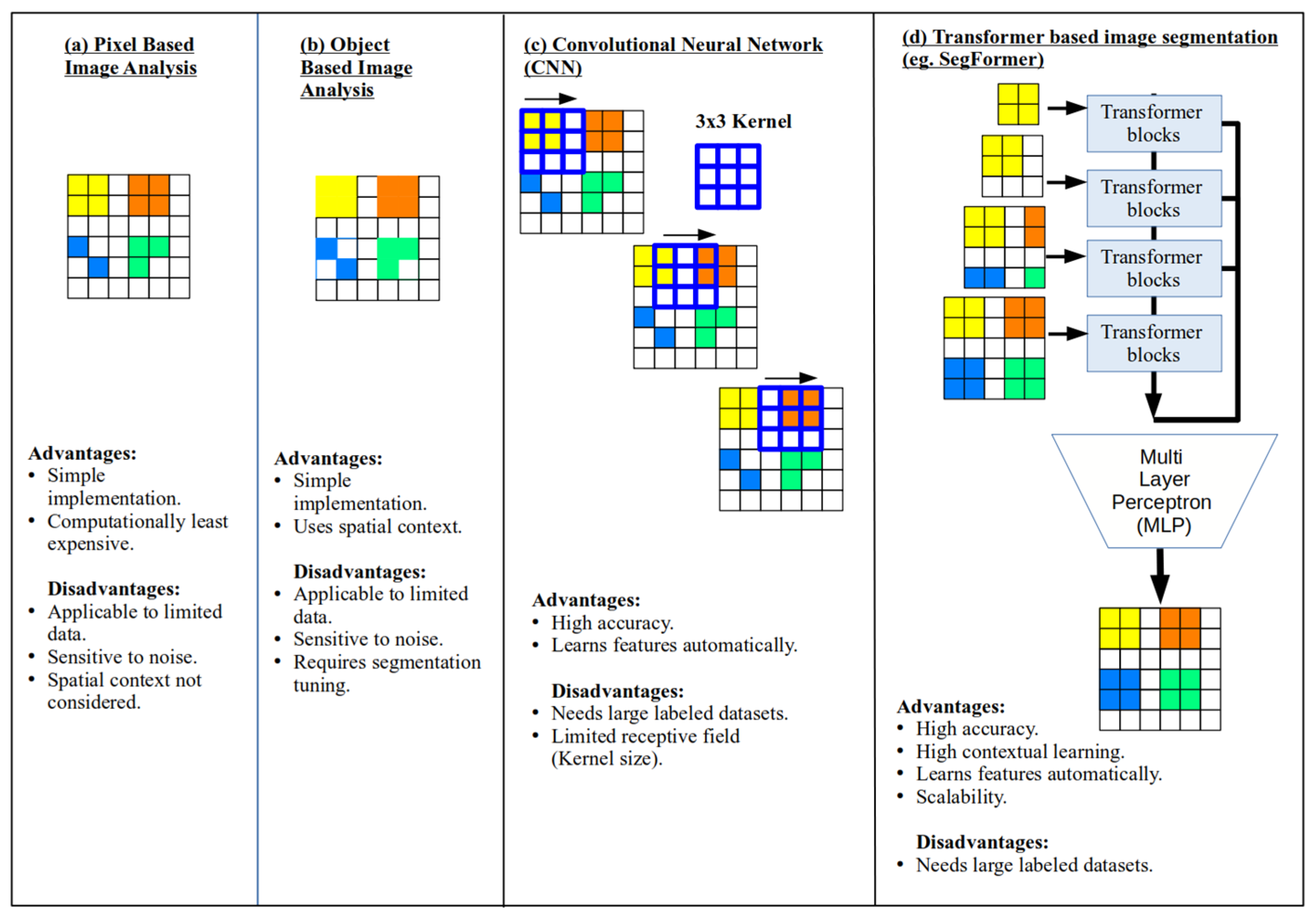
1. Introduction
2. Materials and Methods
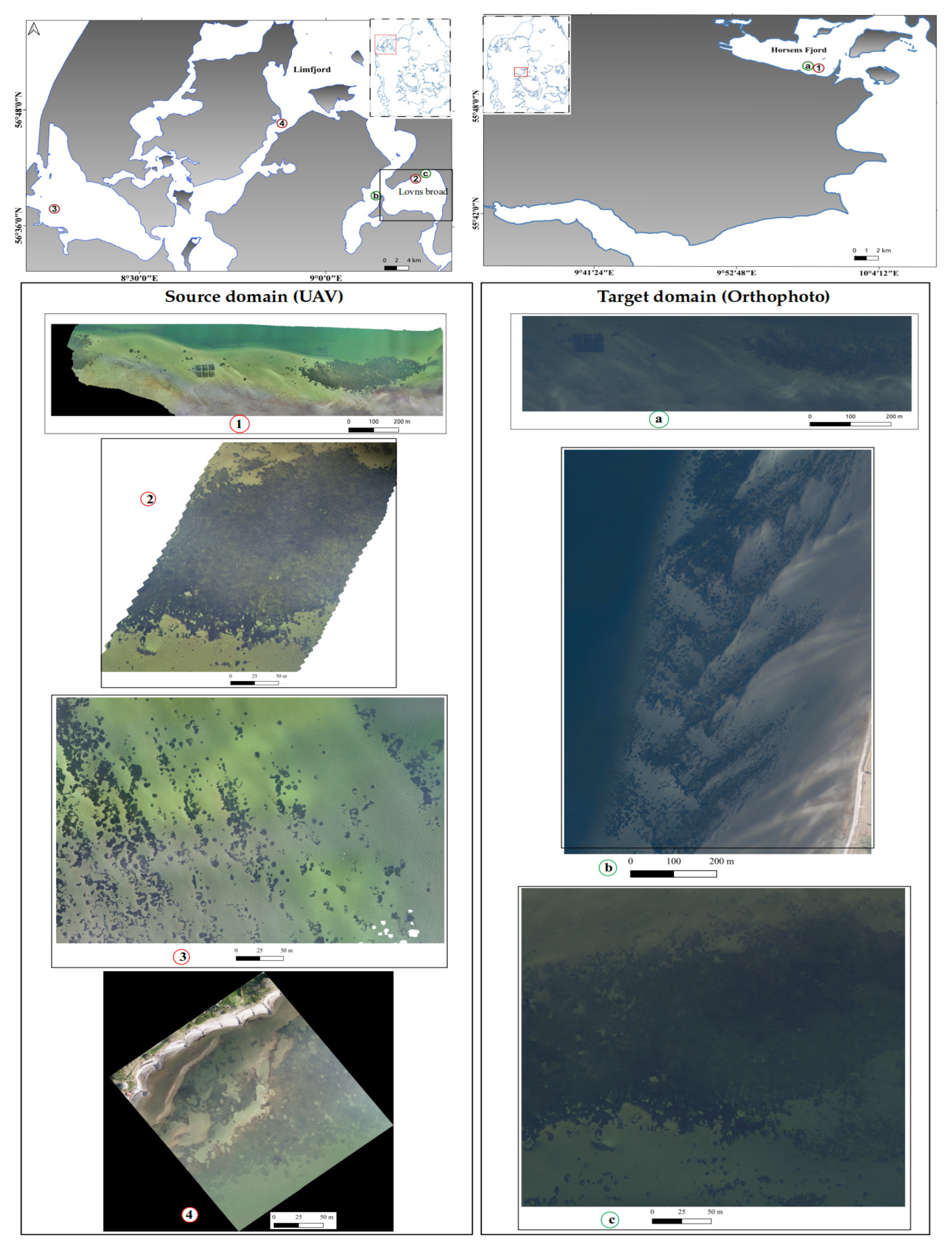
2.1. Source and Target Images
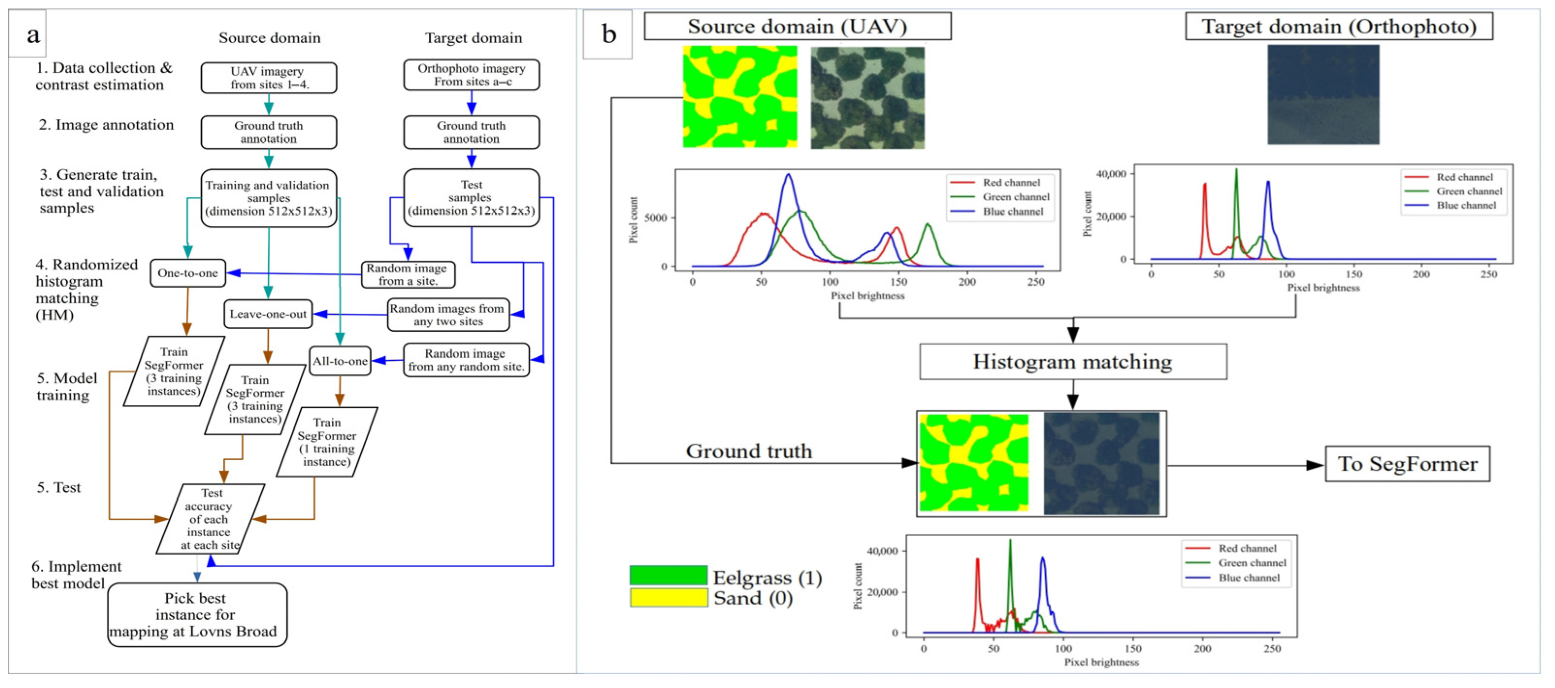
2.2. Training Data Preparation
2.3. Histogram Matching (HM) with SegFormer
2.4. Experimental Setup
- In the one-to-one approach, images from a single site were used for random histogram matching and were tested across all three test sites.
- In the leave-one-out approach, images from two sites were used for histogram matching, while the third site served as the test domain.
- In the all-to-all approach, images from all the sites were used collectively.
2.5. Accuracy Assessment and Domain Alignment Comparison
3. Results
3.1. One-to-One Tests
3.2. Leave-One-Out
3.3. All-to-One
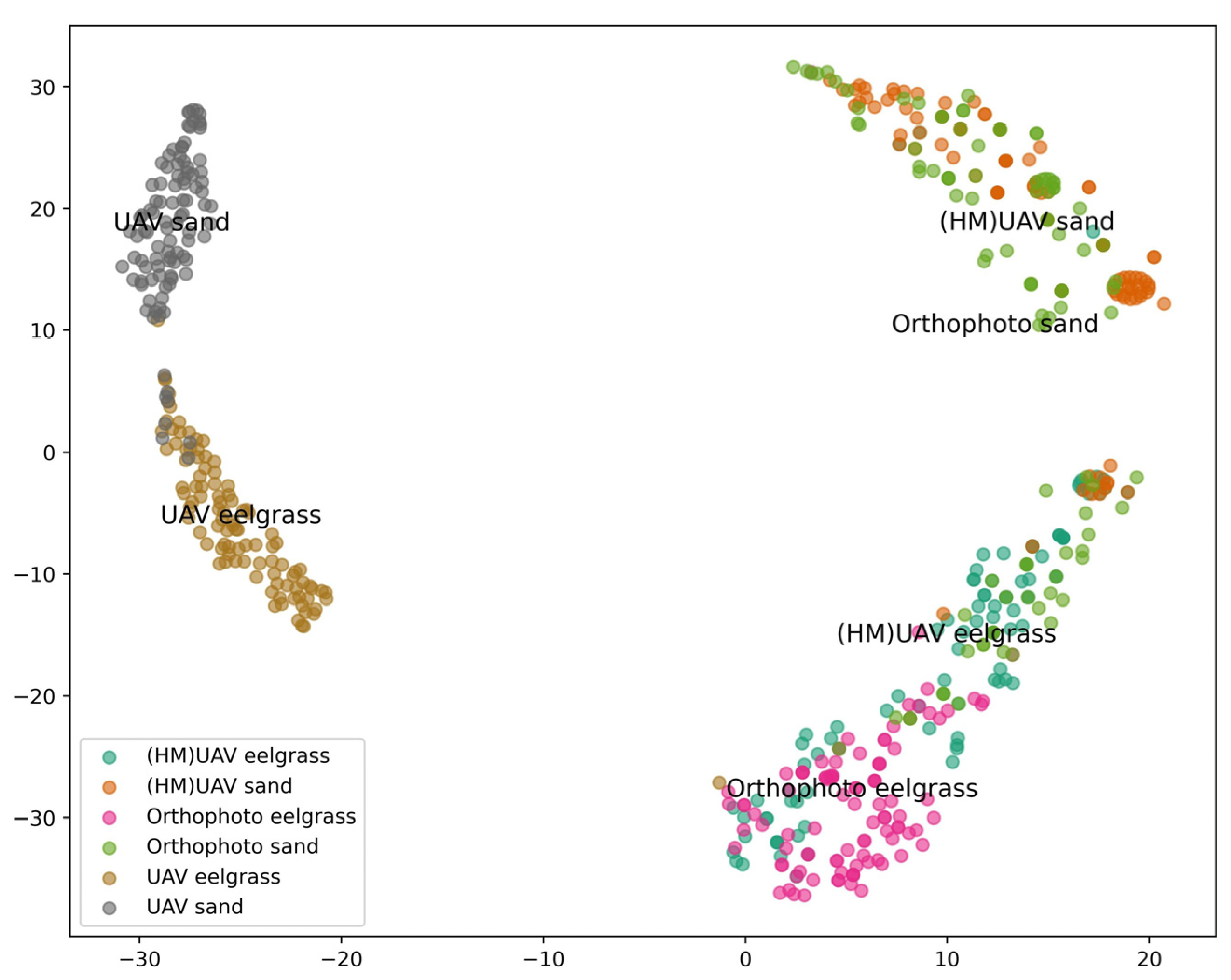
3.4. Domain Alignment Comparison and Limitations
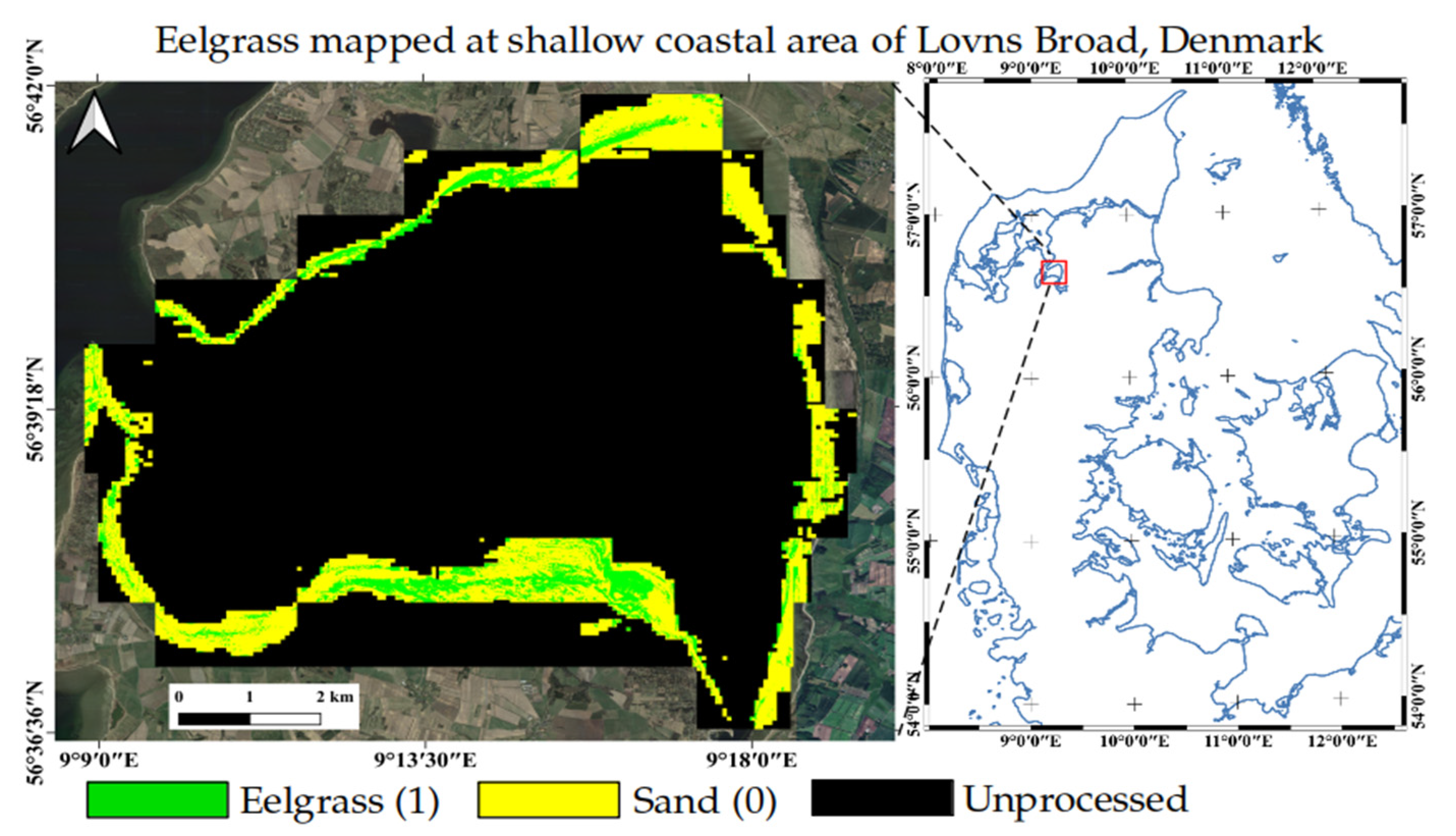
3.5. Model Implementation at Lovns Broad
4. Discussion
4.1. Limitations and Constraints
4.2. Potential for Coastal Habitat Mapping
5. Conclusions
Author Contributions
Funding
Data Availability Statement
Conflicts of Interest
Appendix A. Annotation Protocol for the Segmentation of Shallow Water Eelgrass Habitats
- Image selection:
- 2.
- Reproject to UTM:
- 3.
- Use of in situ observations:
- 4.
- Set the visualization for annotation:
- 5.
- Inclusion/exclusion:
- 6.
- Create vector annotations in the UTM projection:
- 7.
- Check the spatial overlap of the raster:
References
- Barbier, E.B.; Hacker, S.D.; Kennedy, C.; Koch, E.W.; Stier, A.C.; Silliman, B.R. The Value of Estuarine and Coastal Ecosystem Services. Ecol. Monogr. 2011, 81, 169–193. [Google Scholar] [CrossRef]
- Duarte, C.M.; Cebrián, J. The Fate of Marine Autotrophic Production. Limnol. Oceanogr. 1996, 41, 1758–1766. [Google Scholar] [CrossRef]
- Duffy, J.E.; Benedetti-Cecchi, L.; Trinanes, J.; Muller-Karger, F.E.; Ambo-Rappe, R.; Boström, C.; Buschmann, A.H.; Byrnes, J.; Coles, R.G.; Creed, J.; et al. Toward a Coordinated Global Observing System for Seagrasses and Marine Macroalgae. Front. Mar. Sci. 2019, 6, 317. [Google Scholar] [CrossRef]
- Cole, S.G.; Moksnes, P.O. Valuing Multiple Eelgrass Ecosystem Services in Sweden: Fish Production and Uptake of Carbon and Nitrogen. Front. Mar. Sci. 2016, 2, 121. [Google Scholar] [CrossRef]
- Plummer, M.L.; Harvey, C.J.; Anderson, L.E.; Guerry, A.D.; Ruckelshaus, M.H. The Role of Eelgrass in Marine Community Interactions and Ecosystem Services: Results from Ecosystem-Scale Food Web Models. Ecosystems 2013, 16, 237–251. [Google Scholar] [CrossRef]
- Griffiths, L.L.; Connolly, R.M.; Brown, C.J. Critical Gaps in Seagrass Protection Reveal the Need to Address Multiple Pressures and Cumulative Impacts. Ocean Coast. Manag. 2020, 183, 104946. [Google Scholar] [CrossRef]
- Orth, R.J.; Dennison, W.C.; Duarte, C.M.; Fourqurean, J.W.; Heck, K.L.; Hughes, A.R.; Kendrick, G.A.; Kenworthy, W.J.; Short, F.T.; Waycott, M.; et al. A Global Crisis for Seagrass Ecosystems. Bioscience 2006, 56, 987–996. [Google Scholar] [CrossRef]
- Valdemarsen, T.; Canal-Verges, P.; Kristensen, E.; Holmer, M.; Kristiansen, M.D.; Flindt, M.R. Vulnerability of Zostera marina Seedlings to Physical Stress. Mar. Ecol. Prog. Ser. 2010, 418, 119–130. [Google Scholar] [CrossRef]
- Waycott, M.; Duarte, C.M.; Carruthers, T.J.B.; Orth, R.J.; Dennison, W.C.; Olyarnik, S.; Calladine, A.; Fourqurean, J.W.; Heck, K.L.; Hughes, A.R.; et al. Accelerating Loss of Seagrasses across the Globe Threatens Coastal Ecosystems. Proc. Natl. Acad. Sci. USA 2009, 106, 12377–12381. [Google Scholar] [CrossRef] [PubMed]
- Lønborg, C.; Thomasberger, A.; Stæhr, P.A.U.; Stockmarr, A.; Sengupta, S.; Rasmussen, M.L.; Nielsen, L.T.; Hansen, L.B.; Timmermann, K. Submerged Aquatic Vegetation: Overview of Monitoring Techniques Used for the Identification and Determination of Spatial Distribution in European Coastal Waters. Integr. Environ. Assess. Manag. 2021, 18, 892–908. [Google Scholar] [CrossRef] [PubMed]
- Larkum, A.W.D.; Kendrick, G.A.; Ralph, P.J. Seagrasses of Australia: Structure, Ecology and Conservation; Springer: Cham, Switzerland, 2018; ISBN 9783319713540. [Google Scholar]
- Thomasberger, A.; Nielsen, M.M.; Flindt, M.R.; Pawar, S.; Svane, N. Comparative Assessment of Five Machine Learning Algorithms for Supervised Object-Based Classification of Submerged Seagrass Beds Using High-Resolution UAS Imagery. Remote Sens. 2023, 15, 3600. [Google Scholar] [CrossRef]
- Ahmed, S.F.; Bin Alam, M.S.; Hassan, M.; Rozbu, M.R.; Ishtiak, T.; Rafa, N.; Mofijur, M.; Shawkat Ali, A.B.M.; Gandomi, A.H. Deep Learning Modelling Techniques: Current Progress, Applications, Advantages, and Challenges. Artif. Intell. Rev. 2023, 56, 13521–13617. [Google Scholar] [CrossRef]
- Tallam, K.; Nguyen, N.; Ventura, J.; Fricker, A.; Calhoun, S.; O’Leary, J.; Fitzgibbons, M.; Robbins, I.; Walter, R.K. Application of Deep Learning for Classification of Intertidal Eelgrass from Drone-Acquired Imagery. Remote Sens. 2023, 15, 2321. [Google Scholar] [CrossRef]
- Bhatnagar, S.; Gill, L.; Ghosh, B. Drone Image Segmentation Using Machine and Deep Learning for Mapping Raised Bog Vegetation Communities. Remote Sens. 2020, 12, 2602. [Google Scholar] [CrossRef]
- Lowe, S.C.; Misiuk, B.; Xu, I.; Abdulazizov, S.; Baroi, A.R.; Bastos, A.C.; Best, M.; Ferrini, V.; Friedman, A.; Hart, D.; et al. BenthicNet: A Global Compilation of Seafloor Images for Deep Learning Applications. Sci. Data 2025, 12, 230. [Google Scholar] [CrossRef] [PubMed]
- Xie, E.; Wang, W.; Yu, Z.; Anandkumar, A.; Alvarez, J.M.; Luo, P. SegFormer: Simple and Efficient Design for Semantic Segmentation with Transformers. Adv. Neural Inf. Process. Syst. 2021, 15, 12077–12090. [Google Scholar]
- Hoffman, J.; Tzeng, E.; Park, T.; Zhu, J.Y.; Isola, P.; Saenko, K.; Efros, A.A.; Darrell, T. CyCADA: Cycle-Consistent Adversarial Domain Adaptation. In Proceedings of the 35th International Conference on Machine Learning, ICML 2018, Stockholm, Sweden, 10–15 July 2018; Volume 5, pp. 3162–3174. [Google Scholar]
- Islam, K.A.; Hill, V.; Schaeffer, B.; Zimmerman, R.; Li, J. Semi-Supervised Adversarial Domain Adaptation for Seagrass Detection Using Multispectral Images in Coastal Areas. Data Sci. Eng. 2020, 5, 111–125. [Google Scholar] [CrossRef] [PubMed]
- Tasar, O.; Happy, S.L.; Tarabalka, Y.; Alliez, P. ColorMapGAN: Unsupervised Domain Adaptation for Semantic Segmentation Using Color Mapping Generative Adversarial Networks. IEEE Trans. Geosci. Remote Sens. 2020, 58, 7178–7193. [Google Scholar] [CrossRef]
- Thomasberger, A.; Nielsen, M.M. UAV-Based Subsurface Data Collection Using a Low-Tech Ground-Truthing Payload System Enhances Shallow-Water Monitoring. Drones 2023, 7, 647. [Google Scholar] [CrossRef]
- Ghosh Mondal, T.; Shi, Z.; Zhang, H.; Chen, G. Class-Wise Histogram Matching-Based Domain Adaptation in Deep Learning-Based Bridge Element Segmentation. J. Civ. Struct. Health Monit. 2025, 15, 1973–1989. [Google Scholar] [CrossRef]
- Maxwell, A.E.; Warner, T.A.; Guillén, L.A. Accuracy Assessment in Convolutional Neural Network-Based Deep Learning Remote Sensing Studies—Part 2: Recommendations and Best Practices. Remote Sens. 2021, 13, 2450. [Google Scholar] [CrossRef]
- McKenzie, L.J.; Langlois, L.A.; Roelfsema, C.M. Improving Approaches to Mapping Seagrass within the Great Barrier Reef: From Field to Spaceborne Earth Observation. Remote Sens. 2022, 14, 2604. [Google Scholar] [CrossRef]
- Hamad, I.Y.; Staehr, P.A.U.; Rasmussen, M.B.; Sheikh, M. Drone-Based Characterization of Seagrass Habitats in the Tropical Waters of Zanzibar. Remote Sens. 2022, 14, 680. [Google Scholar] [CrossRef]
- Krause, J.R.; Hinojosa-Corona, A.; Gray, A.B.; Watson, E.B. Emerging Sensor Platforms Allow for Seagrass Extent Mapping in a Turbid Estuary and from the Meadow to Ecosystem Scale. Remote Sens. 2021, 13, 3861. [Google Scholar] [CrossRef]
- Tahara, S.; Sudo, K.; Yamakita, T.; Nakaoka, M. Species Level Mapping of a Seagrass Bed Using an Unmanned Aerial Vehicle and Deep Learning Technique. PeerJ 2022, 10, e14017. [Google Scholar] [CrossRef] [PubMed]
- Carpenter, S.; Byfield, V.; Felgate, S.L.; Price, D.M.; Andrade, V.; Cobb, E.; Strong, J.; Lichtschlag, A.; Brittain, H.; Barry, C.; et al. Using Unoccupied Aerial Vehicles (UAVs) to Map Seagrass Cover from Sentinel-2 Imagery. Remote Sens. 2022, 14, 477. [Google Scholar] [CrossRef]
- Price, D.M.; Felgate, S.L.; Huvenne, V.A.I.; Strong, J.; Carpenter, S.; Barry, C.; Lichtschlag, A.; Sanders, R.; Carrias, A.; Young, A.; et al. Quantifying the Intra-Habitat Variation of Seagrass Beds with Unoccupied Aerial Vehicles (UAVs). Remote Sens. 2022, 14, 480. [Google Scholar] [CrossRef]
- Jessin, J.; Heinzlef, C.; Long, N.; Serre, D. A Systematic Review of UAVs for Island Coastal Environment and Risk Monitoring: Towards a Resilience Assessment. Drones 2023, 7, 206. [Google Scholar] [CrossRef]
- Elma, E.; Gaulton, R.; Chudley, T.R.; Scott, C.L.; East, H.K.; Westoby, H.; Fitzsimmons, C. Evaluating UAV-Based Multispectral Imagery for Mapping an Intertidal Seagrass Environment. Aquat. Conserv. Mar. Freshw. Ecosyst. 2024, 34, e4230. [Google Scholar] [CrossRef]
- Roelfsema, C.M.; Lyons, M.; Kovacs, E.M.; Maxwell, P.; Saunders, M.I.; Samper-Villarreal, J.; Phinn, S.R. Multi-Temporal Mapping of Seagrass Cover, Species and Biomass: A Semi-Automated Object Based Image Analysis Approach. Remote Sens. Environ. 2014, 150, 172–187. [Google Scholar] [CrossRef]
- Nahirnick, N.K.; Reshitnyk, L.; Campbell, M.; Hessing-Lewis, M.; Costa, M.; Yakimishyn, J.; Lee, L. Mapping with Confidence; Delineating Seagrass Habitats Using Unoccupied Aerial Systems (UAS). Remote Sens. Ecol. Conserv. 2019, 5, 121–135. [Google Scholar] [CrossRef]
- Yaras, C.; Kassaw, K.; Huang, B.; Bradbury, K.; Malof, J.M. Randomized Histogram Matching: A Simple Augmentation for Unsupervised Domain Adaptation in Overhead Imagery. IEEE J. Sel. Top. Appl. Earth Obs. Remote Sens. 2024, 17, 1988–1998. [Google Scholar] [CrossRef]
- Huber, S.; Hansen, L.B.; Nielsen, L.T.; Rasmussen, M.L.; Sølvsteen, J.; Berglund, J.; Paz von Friesen, C.; Danbolt, M.; Envall, M.; Infantes, E.; et al. Novel Approach to Large-Scale Monitoring of Submerged Aquatic Vegetation: A Nationwide Example from Sweden. Integr. Environ. Assess. Manag. 2022, 18, 909–920. [Google Scholar] [CrossRef] [PubMed]
- Eriander, L. Light Requirements for Successful Restoration of Eelgrass (Zostera marina L.) in a High Latitude Environment–Acclimatization, Growth and Carbohydrate Storage. J. Exp. Mar. Bio. Ecol. 2017, 496, 37–48. [Google Scholar] [CrossRef]
- Krause-Jensen, D.; Greve, T.M.; Nielsen, K. Eelgrass as a Bioindicator under the European Water Framework Directive. Water Resour. Manag. 2005, 19, 63–75. [Google Scholar] [CrossRef]

| UAV Image Locations (Source Domain) | Orthophoto Image Locations (Target Domain) | ||||||||||||
|---|---|---|---|---|---|---|---|---|---|---|---|---|---|
| Site | Location | Max Depth (m) | Image Area (m2) | Eelgrass Cover (m2) | Percentage of Eelgrass Cover (%) | Month and Year of Collection | Site | Location | Max Depth (m) | Image Area (m2) | Eelgrass Cover (m2) | Percentage of Eelgrass Cover (%) | Year of Collection |
| 1 | Horsens Fjord | 3 | 564,045.2 | 56,280 | 10 | August 2020 | a | Horsens Fjord | 3 | 184,416 | 38,048 | 20.6 | 2023 |
| 2 | Lovns Broad | 1 | 98,675.42 | 40,030.8 | 40 | Feb 2021 | b | Skive Fjord | 2.1 | 728,894.05 | 179,373.09 | 24.06 | 2023 |
| 3 | Nissum Broad | 1.1 | 147,839.6 | 24,284.84 | 16 | July 2020 | c | Lovns Broad | 1 | 98,673.85 | 54,265.54 | 55 | 2021 |
| 4 | Nykøbing Mors | 0.9 | 88,393 | 60,955.23 | 68 | April 2021 | |||||||
| Channels | Source Domain (UAV) | Target Domain (Orthophoto) | |||||
|---|---|---|---|---|---|---|---|
| Horsens Fjord | Lovns Broad | Nissum Broad | Nykøbing Mors | Horsens Fjord | Skive Fjord | Lovns Broad | |
| Red | 1 | 0.95 | 1 | 0.67 | 0.73 | 1 | 0.75 |
| Green | 1 | 0.82 | 0.91 | 0.56 | 0.61 | 0.68 | 0.67 |
| Blue | 0.95 | 0.77 | 0.86 | 0.6 | 0.53 | 0.6 | 0.63 |
| Site | Location | Training and Validation Samples | Site | Location | Test Samples |
|---|---|---|---|---|---|
| 1 | Horsens Fjord | 1756 | a | Horsens Fjord (airplane) | 45 |
| 2 | Lovns Broad | 256 | b | Skive Fjord (airplane) | 169 |
| 3 | Nissum Broad | 661 | c | Lovns Broad (airplane) | 20 |
| 4 | Nykøbing Mors | 148 |
| Test Sites | ||||||
|---|---|---|---|---|---|---|
| a | b | c | ||||
| HM Site | Mean F1 | Mean IoU | Mean F1 | Mean IoU | Mean F1 | Mean IoU |
| a | 0.45 | 0.42 | 0.46 | 0.44 | 0.06 | 0.04 |
| b | 0.43 | 0.4 | 0.43 | 0.4 | 0.11 | 0.08 |
| c | 0.4 | 0.38 | 0.47 | 0.44 | 0.17 | 0.15 |
| HM Sites | Test Site | Mean F1-Score | Mean IoU |
|---|---|---|---|
| b and c | a | 0.32 | 0.31 |
| c and a | b | 0.52 | 0.48 |
| a and b | c | 0.47 | 0.43 |
| Test Sites | Mean F1-Score | Mean IoU |
|---|---|---|
| a | 0.34 | 0.32 |
| b | 0.41 | 0.39 |
| c | 0.07 | 0.05 |
Disclaimer/Publisher’s Note: The statements, opinions and data contained in all publications are solely those of the individual author(s) and contributor(s) and not of MDPI and/or the editor(s). MDPI and/or the editor(s) disclaim responsibility for any injury to people or property resulting from any ideas, methods, instructions or products referred to in the content. |
© 2025 by the authors. Licensee MDPI, Basel, Switzerland. This article is an open access article distributed under the terms and conditions of the Creative Commons Attribution (CC BY) license (https://creativecommons.org/licenses/by/4.0/).
Share and Cite
Pawar, S.; Thomasberger, A.; Bengtson, S.H.; Pedersen, M.; Timmermann, K. Eye in the Sky for Sub-Tidal Seagrass Mapping: Leveraging Unsupervised Domain Adaptation with SegFormer for Multi-Source and Multi-Resolution Aerial Imagery. Remote Sens. 2025, 17, 2518. https://doi.org/10.3390/rs17142518
Pawar S, Thomasberger A, Bengtson SH, Pedersen M, Timmermann K. Eye in the Sky for Sub-Tidal Seagrass Mapping: Leveraging Unsupervised Domain Adaptation with SegFormer for Multi-Source and Multi-Resolution Aerial Imagery. Remote Sensing. 2025; 17(14):2518. https://doi.org/10.3390/rs17142518
Chicago/Turabian StylePawar, Satish, Aris Thomasberger, Stefan Hein Bengtson, Malte Pedersen, and Karen Timmermann. 2025. "Eye in the Sky for Sub-Tidal Seagrass Mapping: Leveraging Unsupervised Domain Adaptation with SegFormer for Multi-Source and Multi-Resolution Aerial Imagery" Remote Sensing 17, no. 14: 2518. https://doi.org/10.3390/rs17142518
APA StylePawar, S., Thomasberger, A., Bengtson, S. H., Pedersen, M., & Timmermann, K. (2025). Eye in the Sky for Sub-Tidal Seagrass Mapping: Leveraging Unsupervised Domain Adaptation with SegFormer for Multi-Source and Multi-Resolution Aerial Imagery. Remote Sensing, 17(14), 2518. https://doi.org/10.3390/rs17142518